Article

Inversion of Two-Dimensional In Situ Stress Field Constrained by Multisource Data: A Case Study of Logging-Seismic Integrated Fault Identification


1
Institute of Geophysical and Geochemical Exploration, Chinese Academy of Geological Sciences, Tianjin 300300, China
2
The National Center of Geological Exploration Technology, Tianjin 300300, China
3
State Key Laboratory of Deep Earth Exploration and Imaging, Institute of Geophysical and Geochemical Exploration, Chinese Academy of Geological Sciences, Tianjin 300300, China
4
School of Geological Engineering and Surveying, Chang’an University, Xi’an 710064, China
*
Author to whom correspondence should be addressed.
Processes 2026, 14(10), 1567; https://doi.org/10.3390/pr14101567
Submission received: 20 March 2026 / Revised: 6 May 2026 / Accepted: 9 May 2026 / Published: 13 May 2026

Abstract

In situ stress field inversion is a fundamental challenge in geothermal resource development, oil and gas exploration, and mine safety assessment. To address the non-uniqueness and limited accuracy of traditional single-data-source inversion approaches, this study proposes a two-dimensional in situ stress field inversion method constrained by multi-source data, based on integrated well-seismic fault identification. By incorporating dynamic and static mechanical parameters from well logs and employing both a combined spring model and an anisotropic model, a fault-constrained stress field inversion framework is established. Deep learning and optimization algorithms are utilized to integrate the vertical constraints from well logging data with the lateral continuity characteristics of seismic data, enabling high-resolution reconstruction of the in situ stress field. Taking the complex fault-developed geothermal field in the Xiong’an New Area of the Jizhong Depression, Bohai Bay Basin, as a case study, the proposed method demonstrates a marked reduction in inversion error and a substantial improvement in both fault localization accuracy and stress characterization reliability.

1. Introduction

The efficient exploration and sustainable development of geothermal resources, as abundant, low-carbon renewable energy sources, are central to the global energy transition. However, the successful exploitation of deep geothermal reservoirs depends critically on a thorough understanding of subsurface geomechanical conditions, among which the accurate characterization of the in situ stress field plays a decisive role [1,2]. In situ stress inversion aims to reconstruct the three-dimensional stress distribution by integrating multi-source geological and geophysical data through numerical or analytical techniques [3]. The stress field governs reservoir fracturing, well pattern deployment, and fluid migration pathways; in complex structural settings such as fault zones and heterogeneous formations, its reliable prediction remains a significant engineering challenge [4,5,6,7].
Inversion from a single data type—either seismic or well-log data—is inherently limited by the resolution and coverage of that source. Seismic data offer broad lateral continuity but suffer from limited vertical resolution, whereas well logs provide decimeter-scale vertical precision yet are spatially sparse [8]. Joint use of these two data types can, in principle, build reliable low-frequency models for improved inversion, but current multi-scale data fusion approaches still exhibit notable deficiencies [9,10]. Existing methods often fail to systematically combine the vertical constraints of well logs with the lateral continuity of seismic data, frequently yielding spatially discontinuous two-dimensional stress fields [11,12]. This directly affects the identification of favorable hydraulic fracturing zones and the optimization of completion designs [13]. As a key element of reservoir stimulation, the effectiveness of fracturing is tightly linked to horizontal well placement, and the location of “sweet spots” is controlled by the coupling between the in situ stress field and natural fracture systems [14]. Principal stress orientation, stress difference coefficient, and fracture density are therefore critical indices for fracability evaluation [15,16].
The core challenges in multi-scale data fusion have not yet been fully resolved. These include significant uncertainties in cross-scale parameter mapping, and the absence of an effective coupling mechanism between anisotropic rock properties and fault structures. Conventional “well log calibration–seismic constraint” frameworks often fail to establish rigorous mathematical and physical relationships for these issues, remaining at the level of empirical combinations rather than adopting a logic-driven methodology grounded in geological–mechanical consistency [17,18,19].
With advances in wireline logging, one-dimensional in situ stress profiling has become a standardized technical workflow: overburden stress is obtained by integrating density logs, while mini-frac and leak-off tests accurately calibrate the minimum horizontal principal stress magnitude [20]. The maximum horizontal stress can be constrained using wellbore failure criteria, and its azimuth can be derived from imaging logs (FMI/EMI) [21]. Numerous empirical and physics-based models (Matthews–Kelly model [22], Anderson model [23], Daines model [24], Newberry model [25], Huang’s empirical model [26], Combined spring model [27], and Anisotropic model [28]) have been developed to compute stress magnitudes from acoustic logs. Although economical and continuous, these models often perform poorly in formations with complex lithology [29]. The fast shear-wave azimuth from dipole sonic logs further provides the orientation of the maximum horizontal principal stress [30].
Accurate hydraulic fracturing design and geomechanical simulation require static mechanical parameters of the rock, which differ systematically from the dynamic ones derived from acoustic measurements [31,32,33]. Many unconventional reservoir rocks, especially shales, exhibit significant elastic anisotropy, with Young’s modulus and Poisson’s ratio varying markedly between the horizontal and vertical directions [34]. The stress field around large fault zones and lithological contrasts further introduces directional variability that must be accounted for in stress inversion [35].
In this paper, a two-dimensional “log calibration–seismic constraint” inversion framework is developed for the carbonate fractured geothermal reservoir in the Jizhong Depression, central-eastern China. By jointly incorporating dynamic and static mechanical parameters, a combined spring model, and a vertical transverse isotropy (VTI) model, the approach explicitly accounts for stress-field anisotropy and cross-scale parameter conversion. A deep learning module (CNN–Transformer) is employed purely to enhance the vertical resolution of seismic velocity profiles, which then feed the geomechanical inversion. The framework optimizes the weighting of multi-source data, achieves cross-scale mapping of the horizontal principal stresses, and produces high-resolution two-dimensional stress profiles that improve geological consistency and explain fault activity patterns in the study area.

2. Construction of a Joint Elasticity Parameter Conversion Model

The maximum and minimum horizontal principal stresses are caused by tectonic movements and are related to factors such as tectonic stress and reservoir pressure [36,37,38]. Therefore, when establishing a model based on logging data for calculating the maximum and minimum horizontal principal stresses, the influence of tectonic stress on reservoir pressure must be considered. In terms of in situ stress calculation, the Matthews–Kelly model and the Anderson model do not consider the influence of tectonic stress. Meanwhile, the Daines model lacks an effective means of predicting the maximum horizontal principal stress, whereas the Newberry model does not consider the deformation mechanism of a formation and is not universally applicable. The combined spring model, as a modification of the Huang empirical model, is widely applied [39]. However, the composite spring model is based on an isotropic medium. In this study, using the composite spring model and the anisotropic model, static elasticity parameters are introduced to consider rock anisotropy, thereby enabling a better evaluation of the maximum and minimum principal stresses in the reservoir.

2.1. Isotropic Stress Evaluation Model

The composite spring model is an improved model proposed on the basis of the analysis of the Huang model [27]. It assumes that a rock is a homogeneous, isotropic elastic body that can be obtained from the generalized Hooke’s law:
σ h = μ 1 μ ( σ v α p p ) + E 1 μ 2 ε h + μ E 1 μ 2 ε H + α p p σ H = μ 1 μ ( σ v α p p ) + E 1 μ 2 ε H + μ E 1 μ 2 ε h + α p p
where σ v is the strata vertical principal stress (MPa), pp is the pore pressure (MPa), α is the Biot coefficient (dimensionless), ε h and ε H are the maximum and minimum tectonic stress coefficients (dimensionless, regional empirical parameter), σ h and σ H , are the maximum and minimum horizontal principal stresses (MPa), E is Young’s modulus in the vertical direction (MPa), and μ is Poisson’s ratio in the vertical direction (dimensionless).
The formula for applying density logging to calculate vertical in situ stress is as follows:
σ v = g ρ h 0 + h 0 h ρ d h × 10 3
Eaton [40] synthesized and analyzed the results of previous research and proposed a pore pressure calculation formula based on the effective stress law:
p p = σ v σ v P w Δ t n Δ t m
where h0 is the starting depth of the target layer (m), ρ represents the density logging results (g/cm3), g indicates gravitational acceleration (9.8 m/s2) ρ is the average density of the overlying rock layer (g/cm3) according to the actual stratigraphic conditions, PW is the static liquid column pressure of the formation water at the depth of the required wells (MPa), calculated as g h 0 h 1.03 d h ; Δ t is the measured acoustic time difference of the ground layer at the depth of the required wells (µs/m); m is the area index, also called the Eaton index, taken as the average value of m = 0.2 from measured data back calculation; Δ t n is the surface acoustic time difference (μs/m). ε H ,   ε h are the maximum and minimum structural stress coefficients.

2.2. Anisotropic Stress Evaluation Model

Given the anisotropy of shale, a new in situ stress model conforming to anisotropic strata is constructed by adding elasticity parameters in different directions while considering the aforementioned basic parameters and anisotropy models [28].
σ h = E 11 E 33 μ 31 1 μ 13 ( σ v α P p ) + E 11 1 μ 13 2 ε h + E 11 μ 13 1 μ 13 2 ε H + α P p σ H = E 11 E 33 μ 31 1 μ 13 ( σ v α P p ) + E 11 1 μ 13 2 ε H + E 11 μ 13 1 μ 13 2 ε h + α P p
where E11 is the Young’s modulus measured from the core of a parallel-laminated surface (MPa), E33 is the Young’s modulus measured from the core of a perpendicular-laminated surface (MPa), μ13 are Poisson’s ratios measured from the core of a parallel-laminated surface (dimensionless), and μ31 is the Poisson’s ratio measured from the core of a perpendicular-laminated surface (dimensionless).
Because the fracturing conditions are better represented by the static elastic parameters, the horizontal maximum and minimum principal stresses calculated using the static stiffness coefficients are closer to the actual situation of the formation and are more conducive for field engineering implementation. Rocks with different stratigraphic structures, under the combined influence of dynamic and static stress environments, show different mechanical response characteristics and unique damage modes [41]. The potential assessment of the fracturing capacity of carbonate rocks without the need for borehole core sample collection can be achieved by analyzing the correlation between dynamic and static elastic parameters and anisotropy, with results showing that both are stress-related. In constructing a detailed characterization of in situ stress in rocks, one should not be limited to the horizontal mean stress tensor but should explore in-depth and quantify the complex variability of the stress field within the rock body with changes in spatial location, stiffness coefficients, and elastic parameters.

2.3. Calculation of Dynamic and Static Elastic Parameters of In Situ Stress

Shale formations can be approximated as vertically transverse isotropic (VTI) media, for which the relationship between stress and strain satisfies the generalized Hooke’s law [42]:
σ i j = C i j k l ε k l
A specific form is given by Equation (6):
σ 11 σ 22 σ 33 σ 23 σ 13 σ 12 = C 11 C 12 C 13 0 0 0 C 12 C 11 C 13 0 0 0 C 13 C 13 C 33 0 0 0 0 0 0 C 44 0 0 0 0 0 0 C 44 0 0 0 0 0 0 C 66 ε 11 ε 22 ε 33 2 ε 23 2 ε 13 2 ε 12
where σ i j is the stress component (dimensionless), ε k l is the strain component (dimensionless), and C i j k l is the stiffness factor matrix (dimensionless).
Using the experimentally measured fast and slow transverse wave velocities and density measurements of the core, the dynamic stiffness coefficients C11d, C33d, C44d, C66d, C12d, and C13d can be further calculated as follows [43]:
C 11 d = ρ V p 2 90 °
C 33 d = ρ V p 2 0 °
C 66 d = ρ V sh 2 90 °
C 44 d = ρ V sv 2 0 °
C 12 d = C 11 d 2 ρ V sh 2 90 °
C 13 d = C 44 d + 4 ρ 2 V p 4 45 ° 2 ρ V p 2 45 ° C 11 d + C 33 d + 2 C 44 d + C 11 d + C 44 d C 33 d + C 44 d
where Vp(0°) is the longitudinal wave propagating parallel to the symmetry axis (km/s), Vp(45°) is the longitudinal wave propagating at 45° to the symmetry axis (km/s), Vp(90°) is the longitudinal wave propagating perpendicular to the symmetry axis (km/s), Vsh(90°) is the transverse wave propagating perpendicular to the symmetry axis (km/s), and Vsv(0°) is the transverse wave propagating parallel to the symmetry axis (km/s).
From the dynamic stiffness coefficients, the dynamic Young’s moduli E11d and E33d with the dynamic Poisson’s ratios μ12d, μ31d, and μ13d in different directions can be obtained [44,45]:
E 11 d = C 11 d + C 13 d 2 C 11 d + C 12 d + C 12 d C 33 d C 12 d + C 13 d 2 C 33 d C 11 d C 13 d 2
E 33 d = C 11 d 2 C 33 d + 2 C 13 d 2 C 12 d 2 C 11 d C 13 d 2 C 33 d C 12 d 2 C 11 d 2 C 12 d 2
μ 31 d = C 13 d C 11 d + C 12 d
μ 13 d = C 13 d C 11 d C 12 d C 33 d C 11 d C 13 d 2
where E11d is the dynamic Young’s modulus measured from parallel-laminated surface cores (MPa), E33d is the dynamic Young’s modulus measured from perpendicular-laminated surface cores (MPa), μ13d are dynamic Poisson’s ratios measured from parallel-laminated surface cores (dimensionless), and μ31d is the dynamic Poisson’s ratio measured from perpendicular-laminated surface cores (dimensionless).
Based on the experimental results of static stiffness coefficients, the static Young’s moduli E11s, E33s, and Es(45°) and the static Poisson’s ratios μ31s, and μ13s of shale can be calculated [46]:
E 11 s = 8 C 66 s C 66 s + C 12 s C 11 s + C 12 s + 2 C 66 s
E 33 s = 2 C 66 s C 33 s C 11 s C 12 s
μ 31 s = C 13 s 2 C 12 s + C 66 s
μ 13 s = 2 C 12 s + C 66 s C 11 s C 12 s 2 C 66 s C 13 s C 11 s + C 12 s + 2 C 66 s
where E11s is the static Young’s modulus measured from parallel bedding plane cores (MPa), E33s is the static Young’s modulus measured from core samples perpendicular to bedding planes (MPa), μ13s are dynamic Poisson’s ratios measured from core samples parallel to bedding planes (dimensionless), μ31s is the dynamic Poisson’s ratio measured from core samples perpendicular to bedding planes (dimensionless).

2.4. A Multiscale Fusion Inversion Method for Two-Dimensional Static Anisotropic In Situ Stress

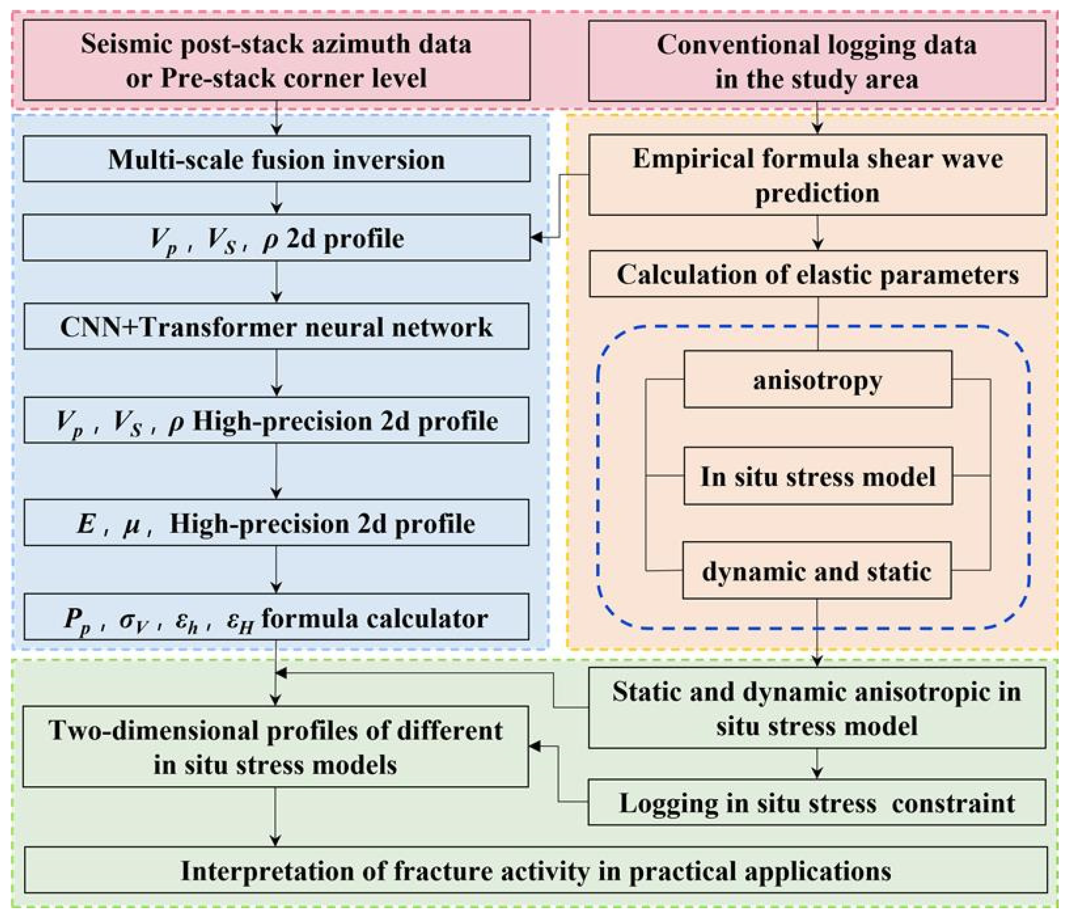
This study is based on poststack seismic data and employs a multiscale fusion inversion technology framework to construct a two-dimensional, high-precision, and static anisotropic in situ stress model. First, conventional two-dimensional velocity–density profile inversion is used to obtain baseline physical property parameters. A depth convolution–Transformer hybrid deep learning architecture is then used to extract nonlinear features and global spatial correlations from seismic data, significantly enhancing the vertical resolution and lateral continuity of velocity, density, and elastic parameter (Poisson’s ratio and Young’s modulus, among others) profiles. Building on these results and using conventional logging data and shear wave predictions predicted using empirical formulas, we establish quantitative calculation models for pore pressure, vertical principal stress, and tectonic stress coefficients using a coupled method that dynamically calibrates elastic parameters while applying static geological constraints, thereby generating high-precision two-dimensional stress profiles and enabling accurate interpretation of fault activity. Figure 1 visually illustrates the testing process of this experiment and the subsequent research approach.

3. Real Data Processing

3.1. Data Sources and Preprocessing

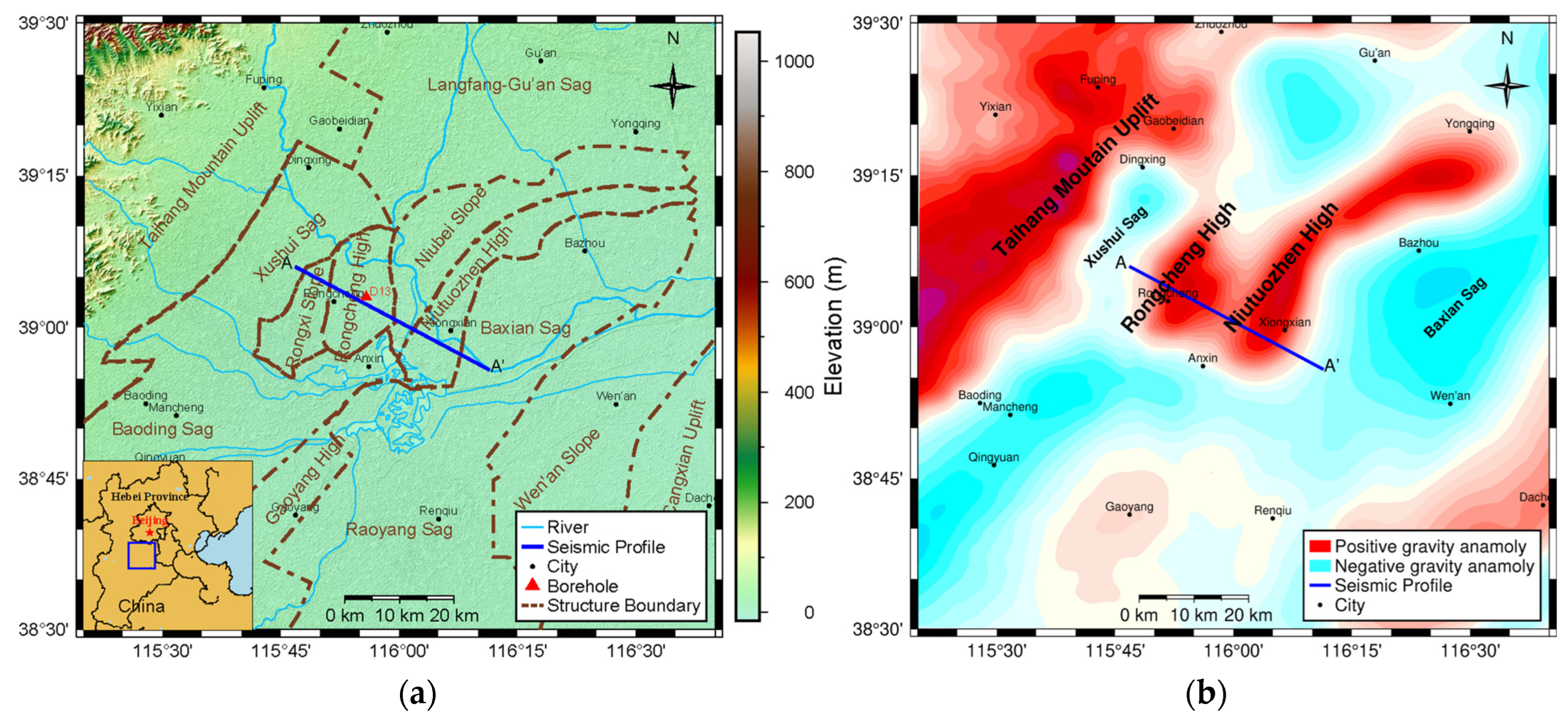
The Xiong’An New Area is situated in the central Jizhong Depression, Bohai Bay Basin, in the middle-eastern region of China (Figure 2). The terrain is nearly flat, with elevation differences of only tens of meters, except for the mountainous northwestern corner. The study area comprises the Rongcheng High, the southern Niutuozhen High, the southern Niubei Slope, and the Baiyangdian Subsag (Figure 2). Structurally, it lies in the transfer zone between the central and northern Jizhong Depression, bounded by the Baoding Sag (southwest), Xushui Sag (northwest), Baxian Sag (southeast), and Raoyang Sag (south). Regionally, it belongs to the eastern block of the North China Craton.
The study area is located in the central tectonic unit of the Jizhong Depression in the Bohai Bay Basin. It encompasses the Rongcheng Uplift, the southern segment of the Niutuozhen Uplift, the southern margin of the Niubei Slope Belt, and the Baiyangdian Depression, among other secondary tectonic units. Its stratigraphic system exhibits the following developmental characteristics from youngest to oldest. The Quaternary Plain Formation is primarily composed of alluvial deposits and exhibits a typical two-part structure: the lower part consists of silt–sand to medium-sand layers, whereas the upper part transitions into sandy clay layers, with a stratigraphic thickness ranging from 348 to 437 m [47]. The Neogene System consists of fluvial clastic rocks, including the Guantiao Formation (0–424.5 m) and the Minghua Town Formation (686–947 m), with a lithological assemblage characterized by alternating sandstone and mudstone layers. The Paleogene System is largely confined to secondary basins and shows significant erosion in the Rongcheng and Niutuo Town uplift zones, resulting in incomplete preservation. Its stratigraphic sequence from top to bottom consists of the Dongying Formation, the Shahuojie Formation, and the Kongdian Formation, with distinct sedimentary discontinuities between each formation. The basement strata include the Middle Proterozoic Great Wall System and the Ji County System, as well as the widely exposed Archean metamorphic rock systems, whose top boundaries exhibit significant spatial variation in burial depth.
Figure 2. Geologic background of the research area. (a) The topography and geological structure of the study area; (b) the residual gravity anomaly of this area, where red corresponds to a positive anomaly and cyan corresponds to a negative anomaly [48].
Processes 14 01567 g002
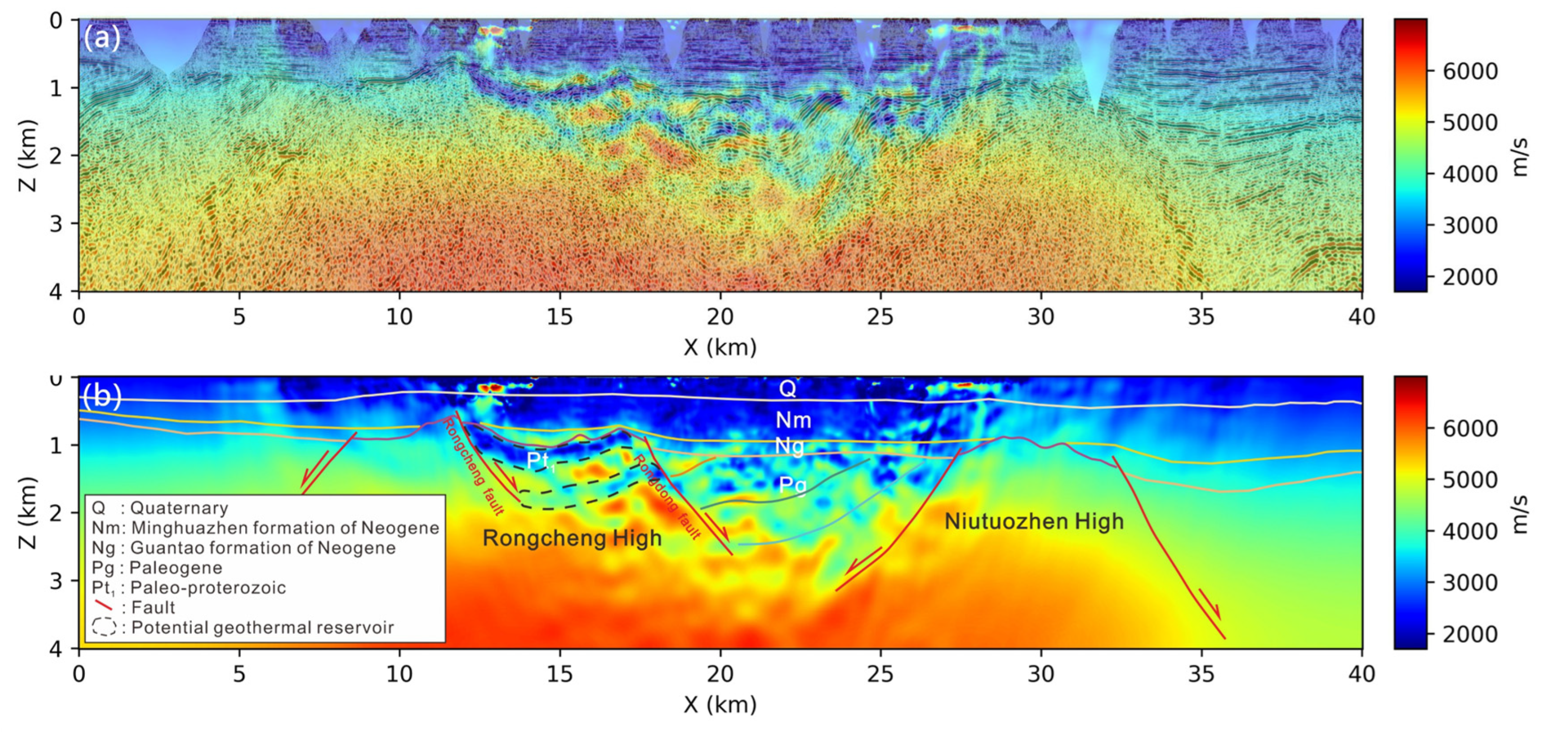
The Jizhong Depression contains multiple geothermal reservoirs characterized by localized low-velocity anomalies. This study employs Laplace–Fourier domain multiscale full-waveform inversion (FWI) technology to obtain high-precision P-wave velocity profiles. First, an iterative traveltime tomography method combined with periodic jump assessment technology was used to construct a high-precision initial velocity model with an initial frequency of 5 Hz. On this basis, the multiscale Laplace–Fourier multiscale FWI method was employed to achieve layer-by-layer velocity modeling. The inversion results were systematically validated through various means, including ray tracing forward modeling, synthetic seismic record calculations, and calibration using neighboring well data, confirming the reliability of the inversion results [48]. The seismic offset profiles and the inverted P-wave velocity model were used to interpret the stratigraphy and faults in the region (Figure 3b). In the velocity model overlying the unconformity surface of the seismic offset profile (Figure 3a), the velocity changes corresponded well with seismic events, validating the reliability of the inversion results and serving as the initial velocity profile selected for this study.
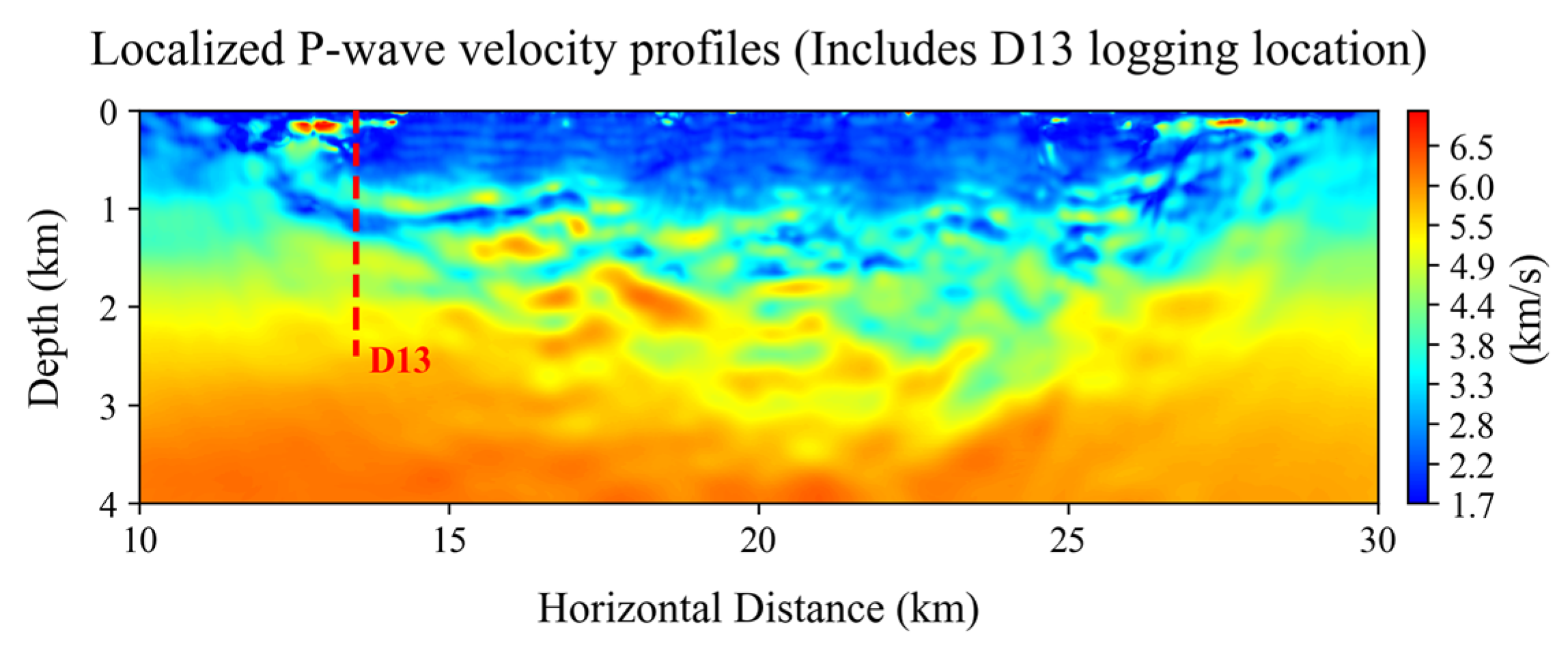
A velocity profile with a length of 20 km and a depth of 4 km was extracted from the central portion of the intersection between the Rongcheng Uplift and the Niutuo Town uplift (Figure 4). The grid spacing in both the horizontal and vertical directions along the profile is 20 m. At the profile location x = 13.5 km, there is a geothermal well (D13) with a depth of 2.5 km. As shown in Figure 5, the inversion results exhibit greater detail in the upper part of the reservoir section and demonstrate good agreement, indicating the accuracy of the inversion.
In geothermal settings, the total stress field can be further influenced by temperature variations. Under the assumption of linear thermo-elasticity, the effective stress incorporates a thermal expansion term:
σ = σ α P p I 3 K β Δ T I
where K is the bulk modulus, β is the linear thermal expansion coefficient, and ΔT is the temperature change relative to a reference state.
Although a detailed temperature field is not directly inverted in the present work, this relationship illustrates how the framework could be extended to account for thermal stresses when additional temperature data become available.

3.2. High-Precision Velocity and Density Profile Calculations with Multisource Data Constraints

P-wave velocity profiles are crucial parameters for characterizing the elastic properties of subsurface media. Traditional acquisition methods primarily rely on two types of data sources. Seismic data have the advantages of strong spatial continuity and broad coverage but are limited by the bandwidth of the acquisition system (10–80 Hz), resulting in relatively low vertical resolution (10–40 m). Meanwhile, logging data can provide high-resolution velocity information at the decimeter level but are limited to the local area around the wellbore. To address the “cross-scale fusion of seismic and logging data,” an end-to-end resolution enhancement framework based on deep learning is employed for full-process prediction.
A depth alignment system between seismic and logging data was established. Cubic spline interpolation was employed to achieve a nonlinear mapping from seismic data to logging depth. This algorithm precisely aligns low-resolution seismic data to the depth coordinates of logging data. A hybrid depth convolution–Transformer model significantly enhanced the vertical resolution of P-wave velocity profiles through multiscale feature encoding, global attention mechanisms, and adaptive normalization. This approach successfully integrated the high-frequency information of logging data while maintaining the lateral continuity of seismic data, providing a new approach for detailed reservoir characterization.
Original seismic data profiles exhibit low vertical resolution, with blurred velocity layer boundaries. Details of velocity changes are scarce, making it difficult to clearly identify thin layers or subtle changes in formation properties. Their lateral continuity is good, but their vertical information is insufficient. Thus, high-resolution logging data curves serve as references, showing high-frequency, high-precision P-wave velocity detail changes. They are capable of resolving fine-scale geological features, such as thin beds, sharp lithological contacts, and small-scale cyclicity, thereby providing high-precision vertical constraints for the inversion framework (Figure 6). However, their data are only distributed discretely at well locations and lack lateral continuity information.

3.2.1. CNN Algorithm

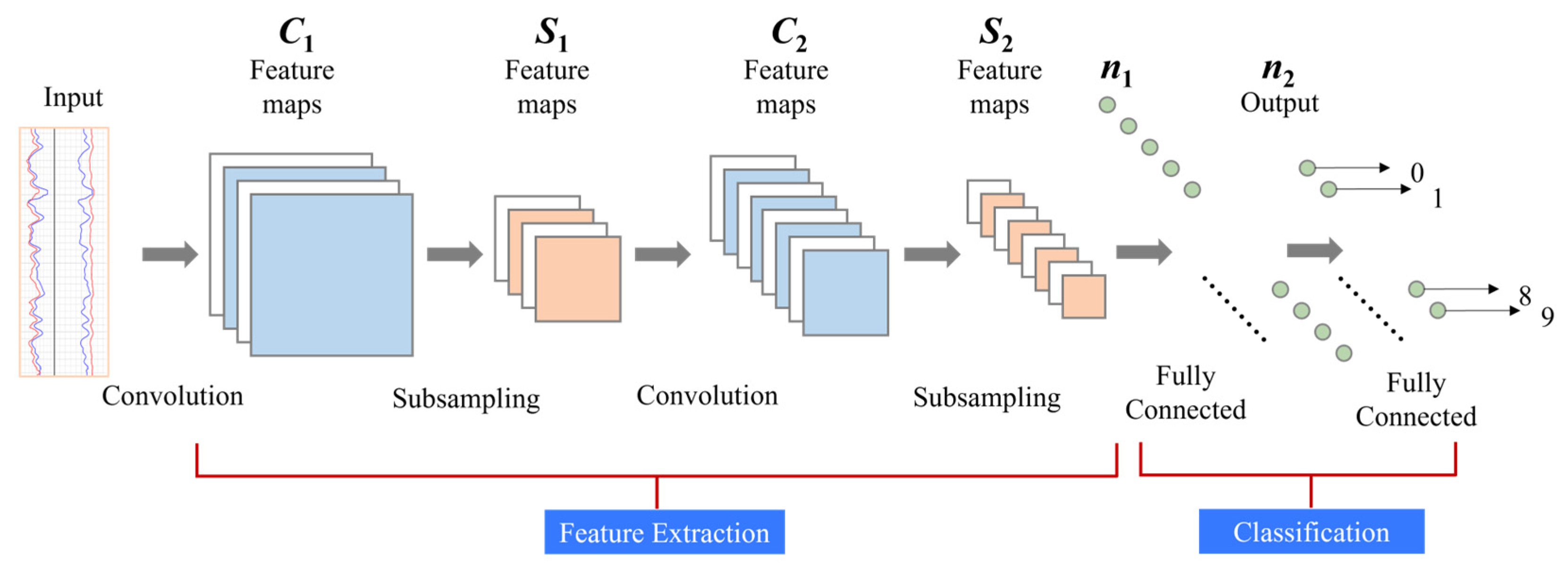
Convolutional neural networks (CNNs) can effectively extract local features from data. They mainly consist of an input layer, a convolution layer, a pooling layer, and a fully connected layer [49]. The convolution layer is responsible for extracting features from input data and performing convolution on data using convolution kernels of different sizes [50]. The convolution network architecture is shown in Figure 7.
A CNN detects local features in input data using its multilayer convolutional structure. Each convolutional layer extracts different levels of features from the data by learning different filter responses, ranging from basic edges and textures to more complex shapes and patterns. These extracted features are processed using activation functions and pooling layers. These not only enhance the model’s nonlinear processing capabilities but also effectively reduce the spatial dimension of the features, thereby reducing computational burden and improving processing efficiency.

3.2.2. Transformer Algorithm

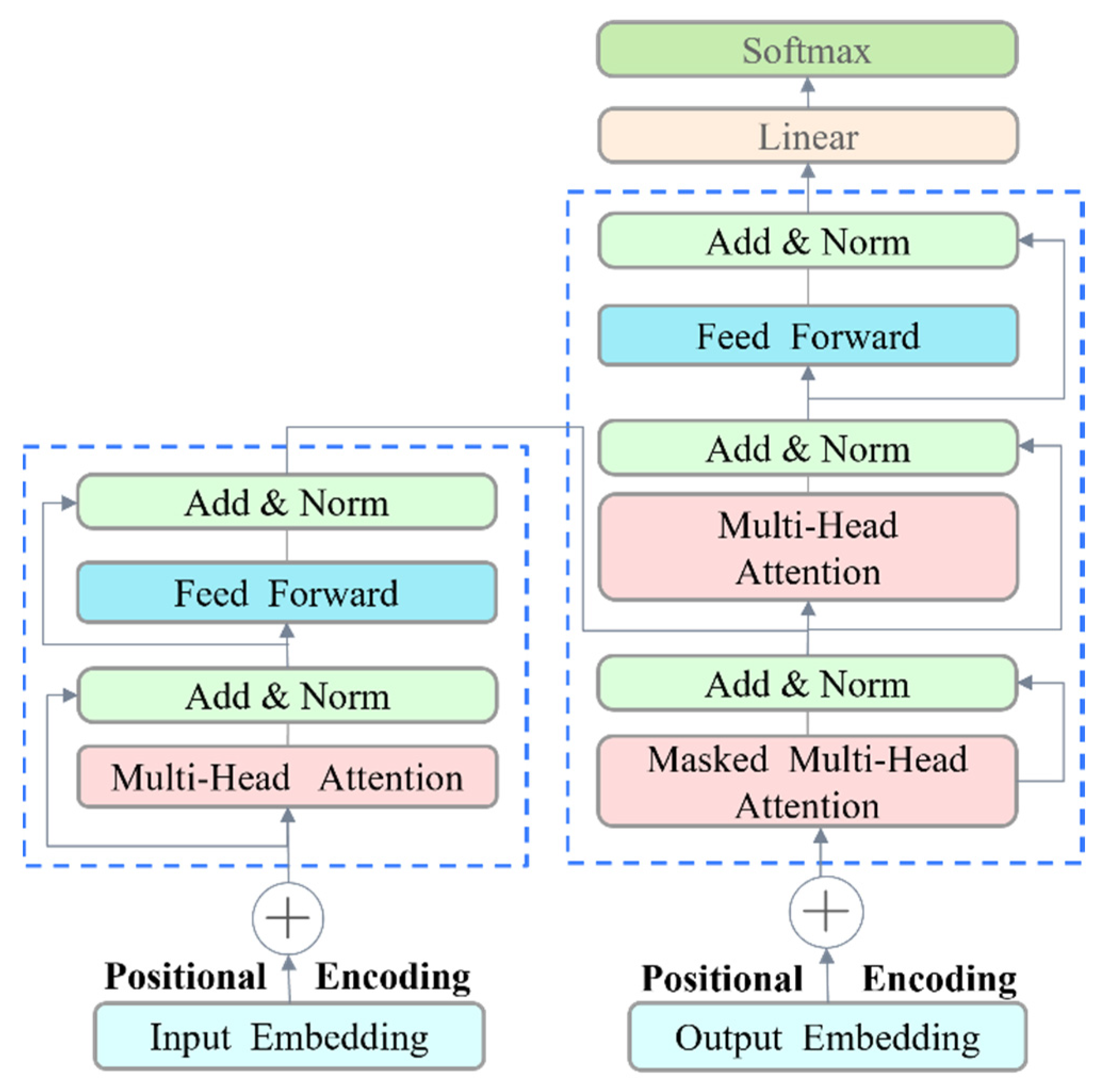
Transformer is a deep learning model based on a self-attention mechanism, proposed by Vaswani [51] et al. It has revolutionized natural language processing and is widely used in tasks such as machine translation, text generation, and language understanding. Unlike traditional recurrent neural networks and long short-term memory networks, Transformer abandons the recurrent structure, relying entirely on the self-attention mechanism to model dependencies between elements in a sequence. This design significantly enhances its parallel computing efficiency and its ability to model long-range dependencies. The Transformer network architecture is shown in Figure 8.
Transformer primarily consists of an encoder and a decoder, each composed of multiple identical layers stacked together. The encoder encodes the input sequence into a continuous representation, whereas the decoder generates the target sequence based on the encoder’s output. The encoder processes the input sequence and generates context vectors. It is composed of multiple identical layers stacked together, with each layer containing two sublayers of multihead self-attention mechanisms. Each sublayer employs residual connections and layer normalization to enhance model training stability and accelerate convergence. Meanwhile, the decoder generates the target sequence based on the context vectors produced by the encoder and previous predictions. Similarly to the encoder, it consists of multiple identical layers stacked together, but each layer has three sublayers: a masked multihead self-attention mechanism, an encoder–decoder attention mechanism, and a feedforward neural network. Similarly, each sublayer includes residual connections and layer normalization.

3.2.3. CNN–Transformer Model

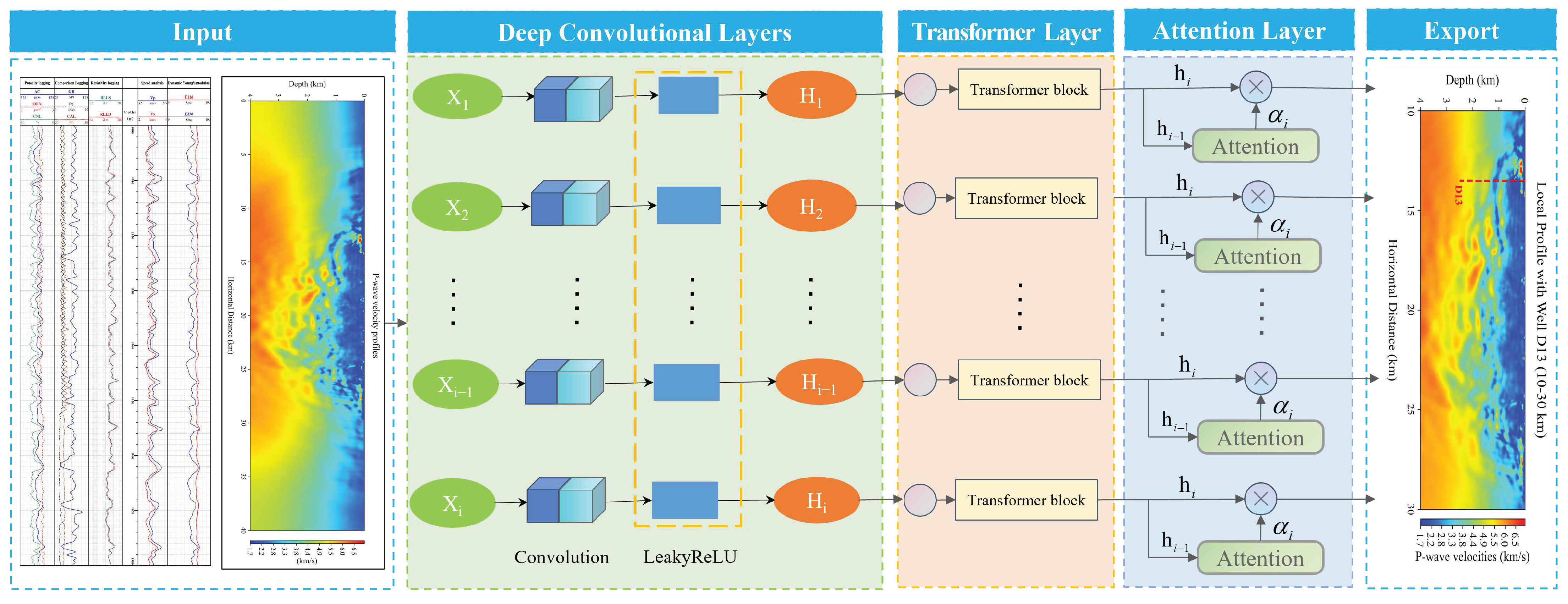
The self-attention mechanism is introduced in the Transformer module to establish long-range dependencies. Breaking through the limitations of traditional CNN or RNN architectures, a hybrid mode of “local convolution + global attention” is adopted. This addresses the excessive reliance of traditional Transformer on the absolute position of sequences and adapts to changes in layer depth. Ultimately, high-resolution two-dimensional seismic velocity profiles are generated, with the specific operational process shown in Figure 9.
The data from both aforementioned sources are converted into digital information, normalized, and processed using a multiscale feature encoder to construct a multiscale feature pyramid using cascaded convolution kernels. The leaky rectified linear unit (LeakyReLU) activation function alleviates the gradient vanishing problem. Group normalization (GN) is used to replace the traditional BatchNorm layer, which normalizes each small batch of data to accelerate neural network training and improve model stability. GN divides channels into multiple groups and normalizes within each group, reducing dependence on batch size (Table 1).
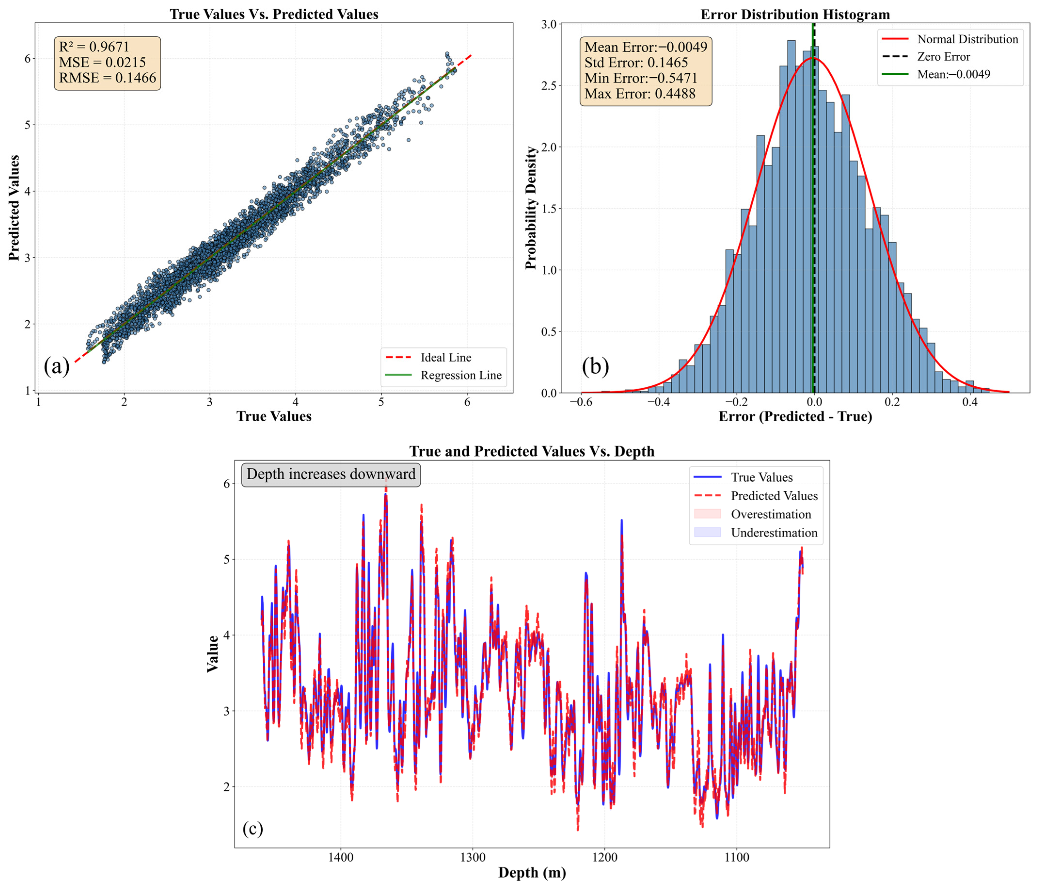
The high-precision P-wave velocity predicted by the deep convolutional–Transformer hybrid model effectively validates the proposed method through intuitive comparison, demonstrating its feasibility in significantly enhancing vertical resolution and successfully integrating high-frequency information. Compared with the original seismic section, the result approaches the detailed level of well-log curves more closely. The steep gradients of velocity variations and high-frequency oscillatory features are effectively recovered. While substantially improving vertical resolution, the prediction result successfully preserves the lateral continuity and structural characteristics inherent in the original seismic data, without introducing unrealistic spatial discontinuities or noise. With an R2 = 0.9671 and MSE = 0.0215, the prediction accuracy exceeds 95%. This close agreement demonstrates the effectiveness of the depth alignment system and hybrid model in accurately mapping and fusing multi-scale data. In summary, Figure 10a–c robustly validate that the proposed fusion method can overcome the vertical resolution limitations of seismic data while maintaining its inherent lateral continuity. It effectively “embeds” the high-frequency, high-resolution velocity information from well-log data into the seismic volume, generating a continuous velocity profile with well-log-scale vertical resolution, thereby establishing a solid data foundation for detailed reservoir characterization.

3.3. A Model for Evaluating the Isotropic Nature of In Situ Stress Based on Dynamic and Static Conditions

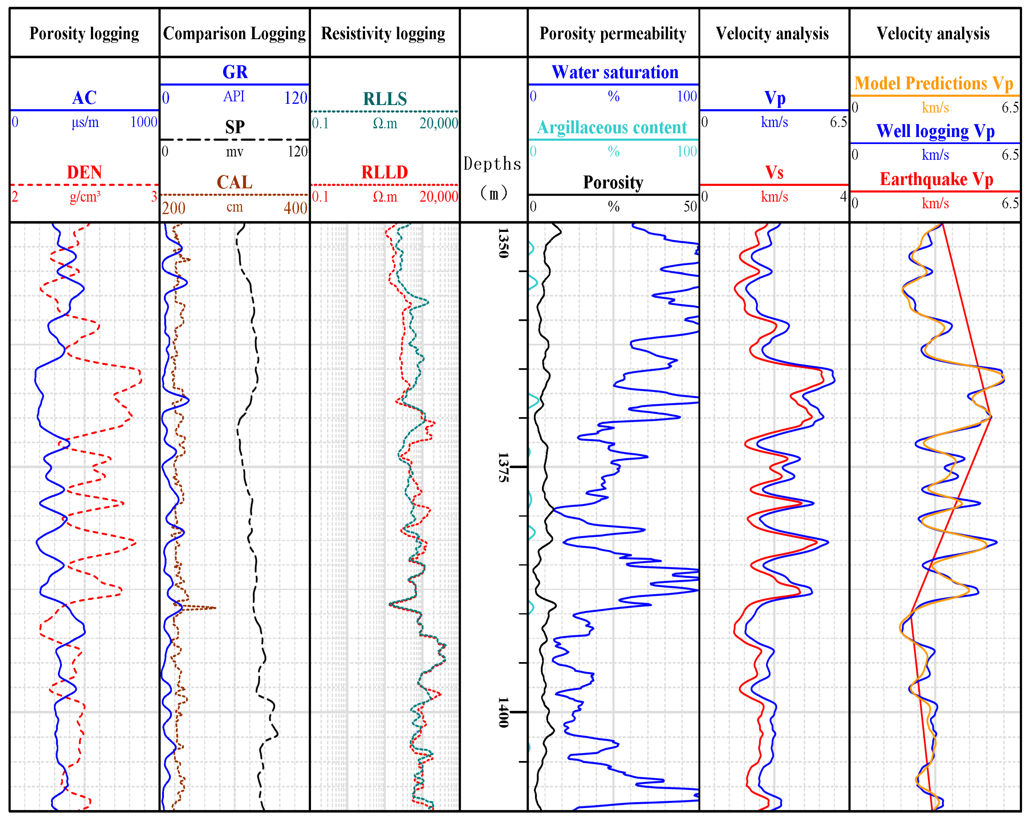
This study investigates an inversion method of rock mechanics parameters based on logging data. Traditional rock mechanics experiments are limited by their discrete sampling, limiting the calibration of rock mass parameters at borehole locations and thus hampering the systematic characterization of mechanical property distribution across multiple rock layers in the vertical direction of the study area. To address this, this study utilized complete logging response sequences (including density, resistivity, and acoustic travel time) from key benchmark wells. By applying rock physics modeling to the logging data, a regional model of vertical rock mechanical parameter profiles for multiple rock types within different tectonic units was constructed. However, most of the discussions focused on the results of ultrasonic measurements [52].
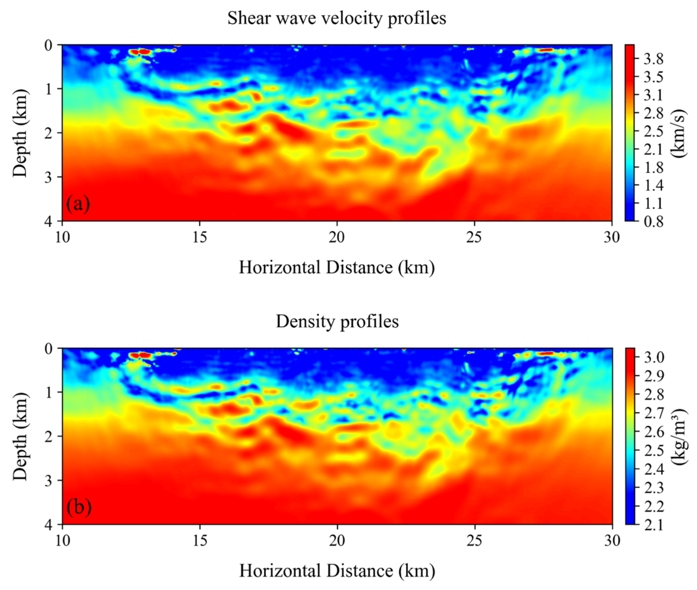
By fitting the relationship between density logging and acoustic logging data from Well D13, the density profile in this study was calculated using Equation (22). Because of systematic gaps in shear wave logging records for most exploration blocks, a shear wave travel time prediction model (Equation (23)) was employed to reconstruct shear wave travel times and calculate dynamic mechanical parameters. The specific shear wave velocity profile is shown in Figure 11.
ρ = 1.85 × V p 0.25
V s = V p 1 1.15 × 1 / ρ + 1 / ρ 3 e 1 / ρ 1.5
where ρ is the density (g/cm3) and e is a natural constant, generally taken as 2.718.
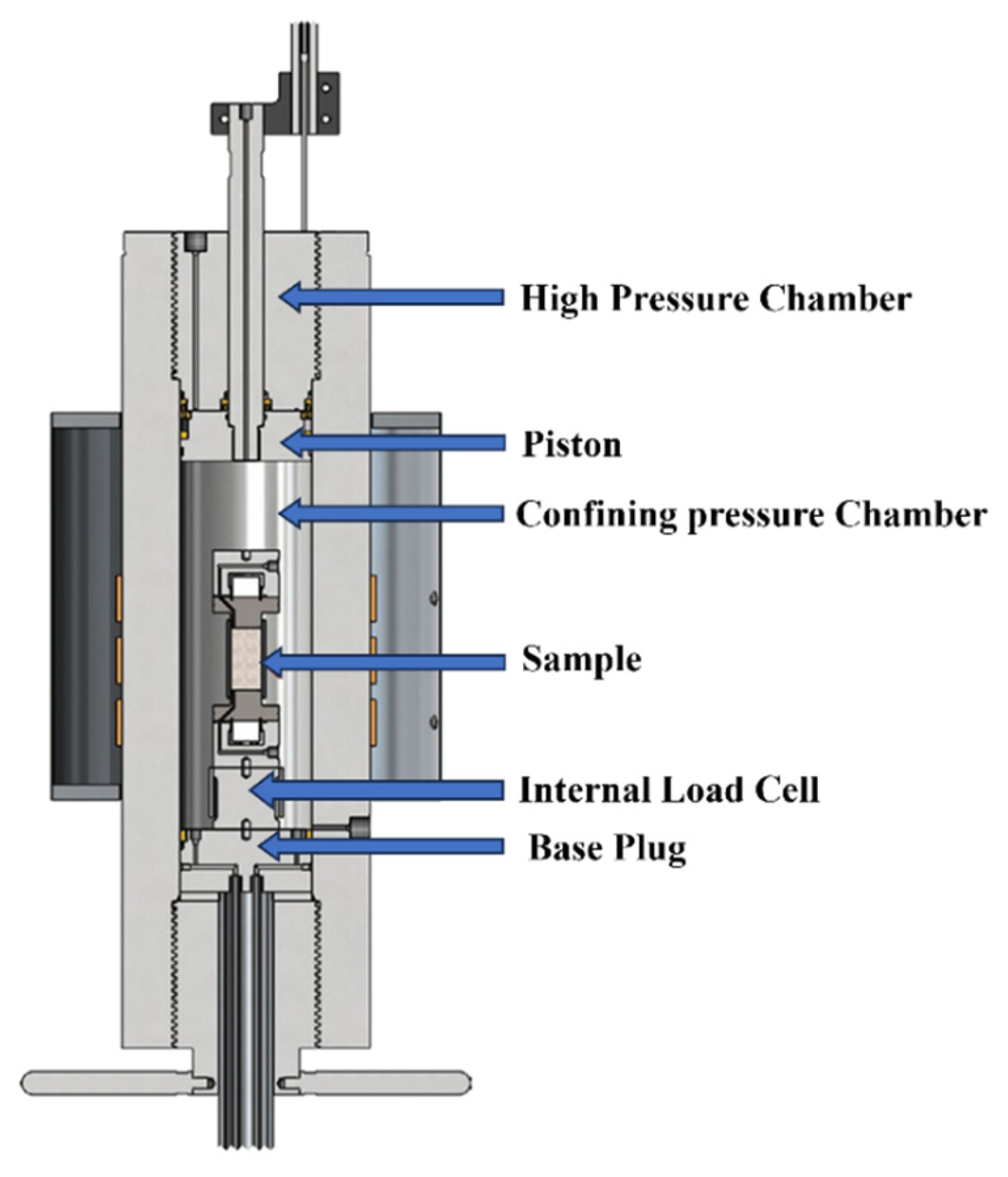
The rock mechanical parameters were characterized using an AutoLab 1500 system from New England Research (NER), based in White River Junction, VT, United States, capable of confining and pore pressures up to 70 MPa and temperatures up to 150 °C. The system enables simultaneous acoustic and mechanical measurements (Figure 12).
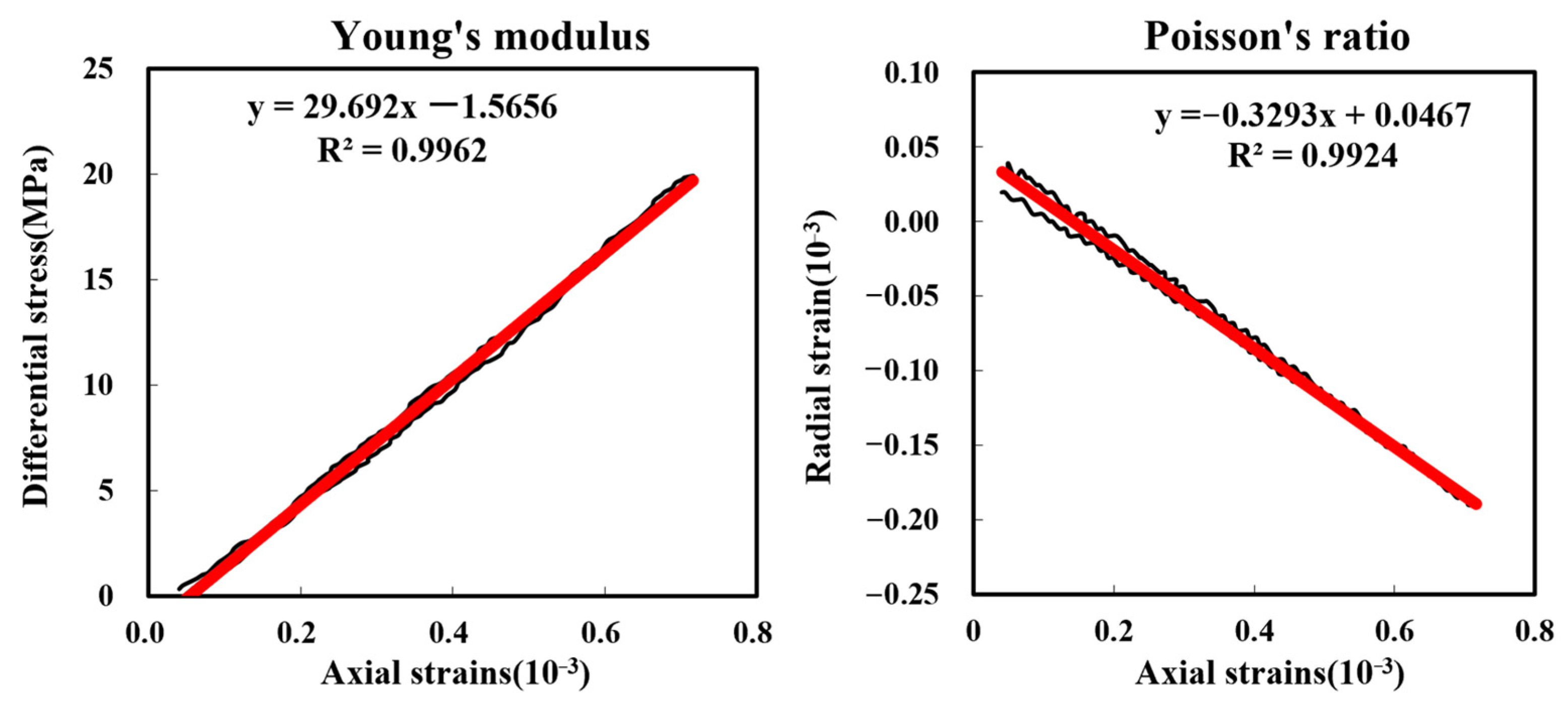
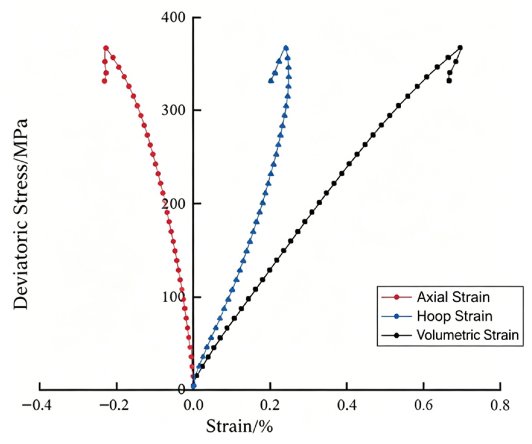
For static testing, a differential stress loading–unloading cycle was applied under a constant confining pressure of 30 MPa at 20 °C. The static Young’s modulus and Poisson’s ratio were determined from the linear-elastic portion of the stress–strain curves recorded at various lamination angles. As an example, Figure 13 yields a static Young’s modulus of 29.69 MPa and a static Poisson’s ratio of 0.329 for one representative sample.
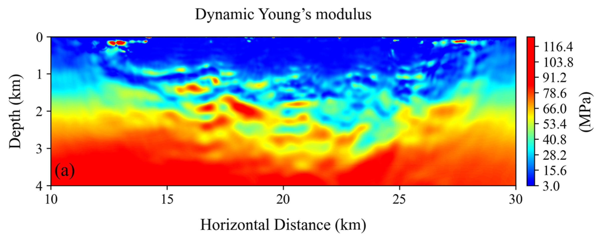
For dynamic testing, P-wave and S-wave velocities were measured on core samples prepared at different angles relative to lamination under triaxial compression at 20 °C. The dynamic Young’s modulus and dynamic Poisson’s ratio were calculated from the measured velocities and bulk density using the standard relations (Equations (24) and (25)), with the results shown in Figure 14a,b.
E d = ρ v s 2 ( 3 v p 2 4 v s 2 ) ( v p 2 v s 2 ) × 10 6
μ d = ( v p 2 2 v s 2 ) 2 ( v p 2 v s 2 )
Because the acoustic-derived dynamic parameters systematically exceed the static ones owing to the high-frequency loading response, a quantitative dynamic-to-static conversion was established via multiple regression on core data matched in the depth domain (Equations (26) and (27)). For the deep carbonate intervals where no core was available, published carbonate-specific conversion formulas were adopted [53], with the fitting results presented in Figure 14c,d.
E s = 0.9578 × E d + 4.4127
μ s = 0.8853 × μ d + 0.0449
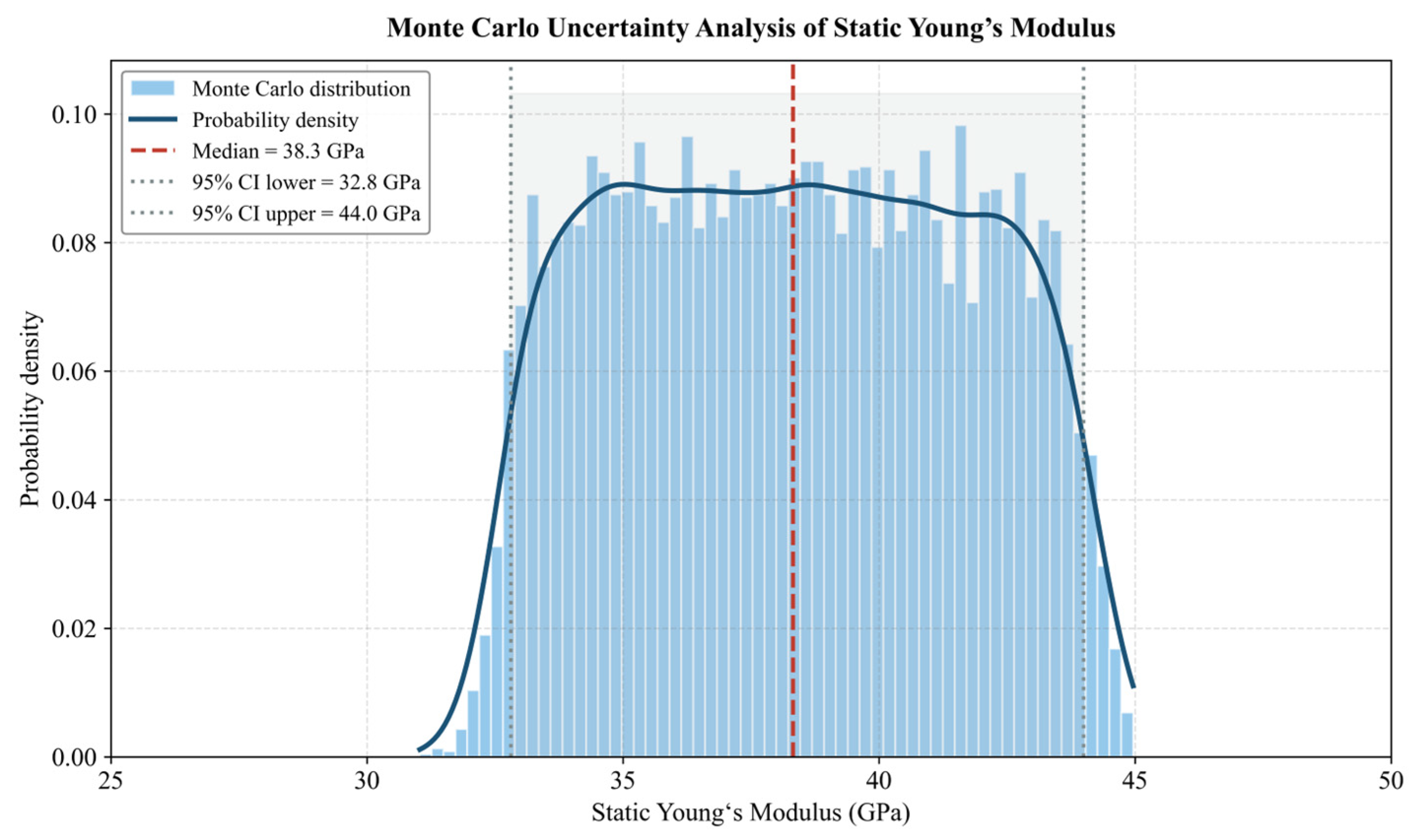
To assess the uncertainty propagated by the dynamic-to-static Young’s modulus conversion, a Monte Carlo simulation was performed using the high-resolution log data from Well D13. A total of 5000 static Young’s modulus values were first derived from the dynamic-to-static empirical relationship (Equation (26)) over the depth range of 1250–1750 m, where the conversion is most reliable. The conversion coefficient was then perturbed uniformly within ±15% of its calibrated value, and a normally distributed measurement noise (σ = 0.5 GPa) was added to simulate random errors. For each of the 10,000 Monte Carlo realizations, new static modulus values were computed for all depth points. The aggregated probability density distribution of the static Young’s modulus is presented in Figure 15. The analysis yields a median value of 38.3 GPa and a 95% confidence interval of 32.8–44.0 GPa, both well below the predetermined upper bound of 45 GPa. These results demonstrate that the static modulus is stably constrained and that the residual uncertainty in the dynamic-to-static conversion does not jeopardize the reliability of the in situ stress inversion.
The fundamental principle of two-dimensional stress inversion is to infer the stress tensor distribution across a profile using observational and constraint data. It is typically assumed that geological strata are in regional equilibrium and that the stress field can be characterized by principal stress directions and stress ratios. Logging data are used to derive strata density and dynamic and static elastic parameters, and vertical principal stresses are calculated. Seismic data provide lateral velocity and fracture information, which are used to infer horizontal stress directions. Under boundary conditions (regional tectonic stress), the magnitude and direction of horizontal principal stresses are adjusted to ensure that the simulation results align with all observational data. This approach yields the distribution characteristics of principal stress directions and stress ratios (e.g., stress difference ratios) along both horizontal and vertical directions, providing a foundation for fault detection.
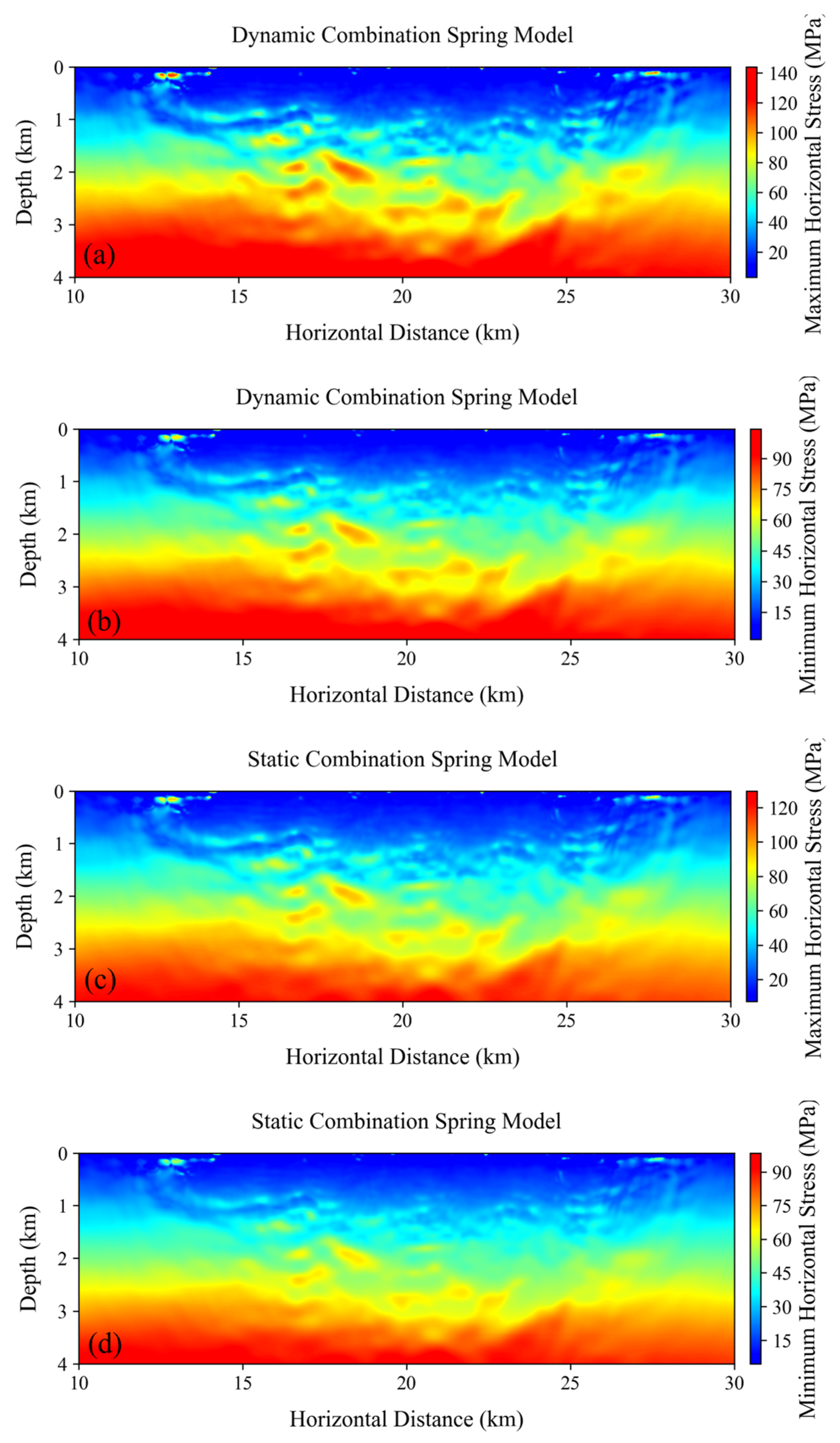
By substituting the two-dimensional dynamic elastic parameter profiles and the fully static elastic parameter profiles calculated above into Equation (1), we can obtain the dynamic combined spring model stress profiles and the static combined spring model stress profiles, respectively, and calculate the maximum and minimum horizontal principal stresses. Generally, distinct zones can be identified: high-stress zones (e.g., tectonic high points and hard strata), low-stress zones (e.g., soft strata and near faults), and areas with sharp changes in stress gradients (e.g., stratigraphic interfaces and salt dome flanks). Typically, both the maximum and minimum horizontal principal stresses increase with depth (linearly or nonlinearly). Additionally, structural stress differences can reveal the significant influence of geological factors such as faults, lithological changes, and structural variations on stress distribution (e.g., stress shielding and stress concentration). Specific effects are shown in Figure 16.

3.4. A Model for Evaluating the Anisotropy of Dynamic and Static In Situ Stress

Without drilling and core sampling, the fracturing capacity of rock layers can potentially be assessed by analyzing the correlation between static and dynamic elastic parameters and anisotropy, with results indicating both as stress-dependent. When constructing a detailed characterization of rock stress, one should go beyond the horizontal mean stress tensor and explore and quantify complex variations in the stress field within the rock body as a function of spatial location, stiffness coefficient, and elastic parameters.
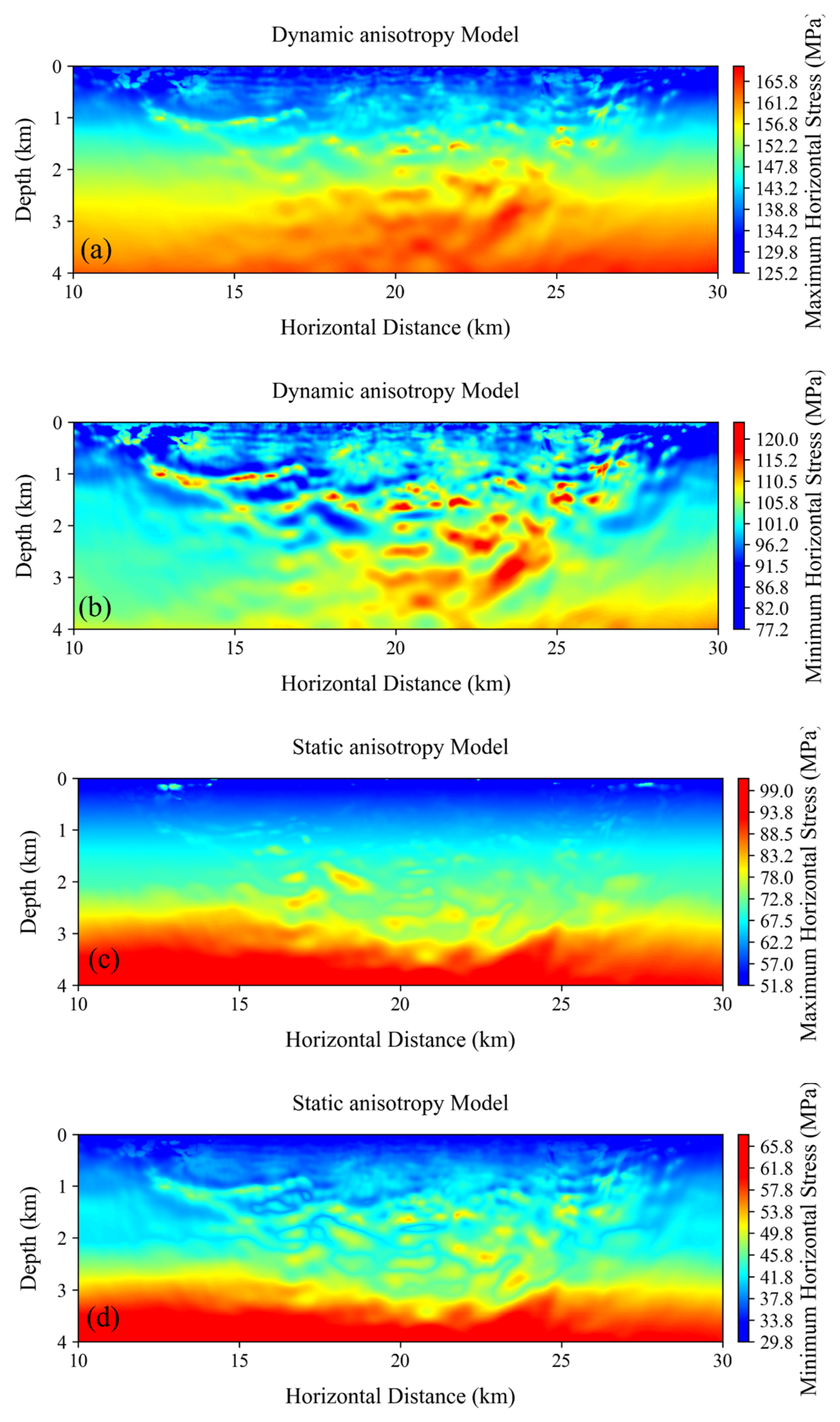
To calculate anisotropic stress, six dynamic stiffness coefficients must primarily be determined—C11d, C33d, C44d, C66d, C12d, and C13d—which can be calculated using Equations (7)–(12) based on the P-wave velocity, fast and slow S-wave velocities, and density. Equations (13)–(16) are then used to obtain the dynamic Young’s moduli E11d and E33d and the dynamic Poisson’s ratios μ31d, and μ13d in different directions, which are subsequently substituted into Equation (4) to calculate the magnitude of the dynamic anisotropic stress model (Figure 17a,b). Research has found that dynamic stiffness coefficients can be converted into static stiffness coefficients. In the laboratory, the conversion formulas (Equations (28)–(33)) for dynamic and static stiffness coefficients were fitted using sample stiffness coefficient measurement results, and the magnitude of static anisotropic stress was then solved.
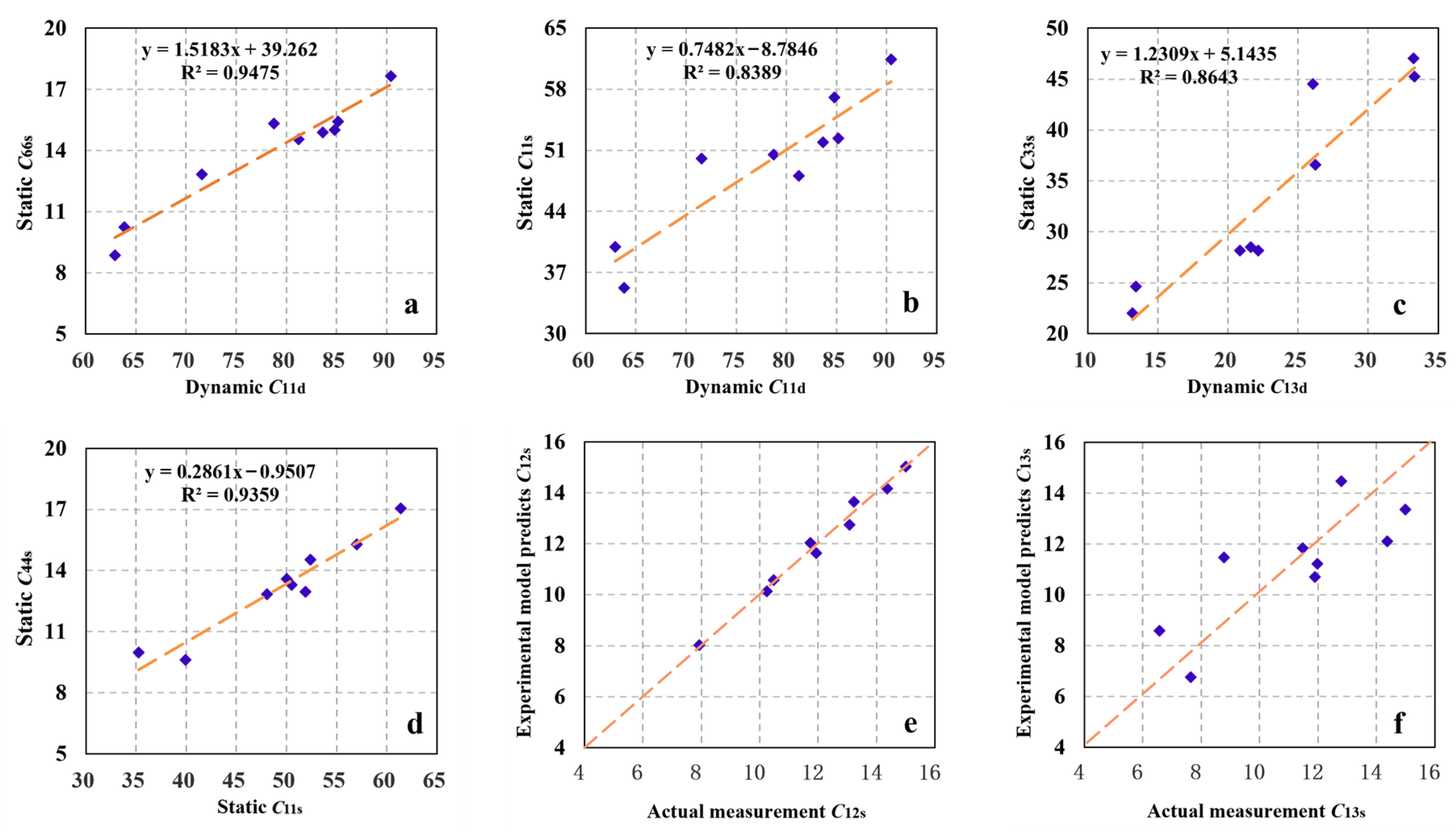
Using triaxial compression tests, the static stiffness coefficients of the rock were derived. The relationship between the static and dynamic stiffness coefficients of the rock was investigated (Figure 18a–d). In laboratory measurements, the static stiffness coefficient C12s shows a certain correlation with C11s and C66s, while C13s exhibits a correlation with C11s and C44s. To accurately characterize these two parameters, a new model was constructed using multiple linear regression. The predictive performance of the two models was compared and analyzed using static stiffness coefficient data calculated from core samples in the study area (Figure 18e,f).
C 66 s = 0.2724 C 11 d 7.4039
C 11 s = 0.7482 C 11 d 8.7846
C 33 s = 1.2309 C 13 d + 5.1435
C 44 s = 0.2861 C 11 s 0.9507
C 12 s = 0.6135 C 11 s 1.3379 C 66 s + 0.1065
C 13 s = 0.3701 C 11 s 0.2789 C 44 s 3.4978
Substituting into Equations (17)–(20) yields the static elastic parameters of the rock (E11s, E33s, μ31s, μ13s). Therefore, investigating the conversion relationship between static and dynamic stiffness coefficients becomes a key issue in calculating the anisotropic stress model. Substituting into Equation (4) yields the magnitude of the static anisotropic stress model (Figure 17c,d).

3.5. Verification of Errors in Different Stress Models

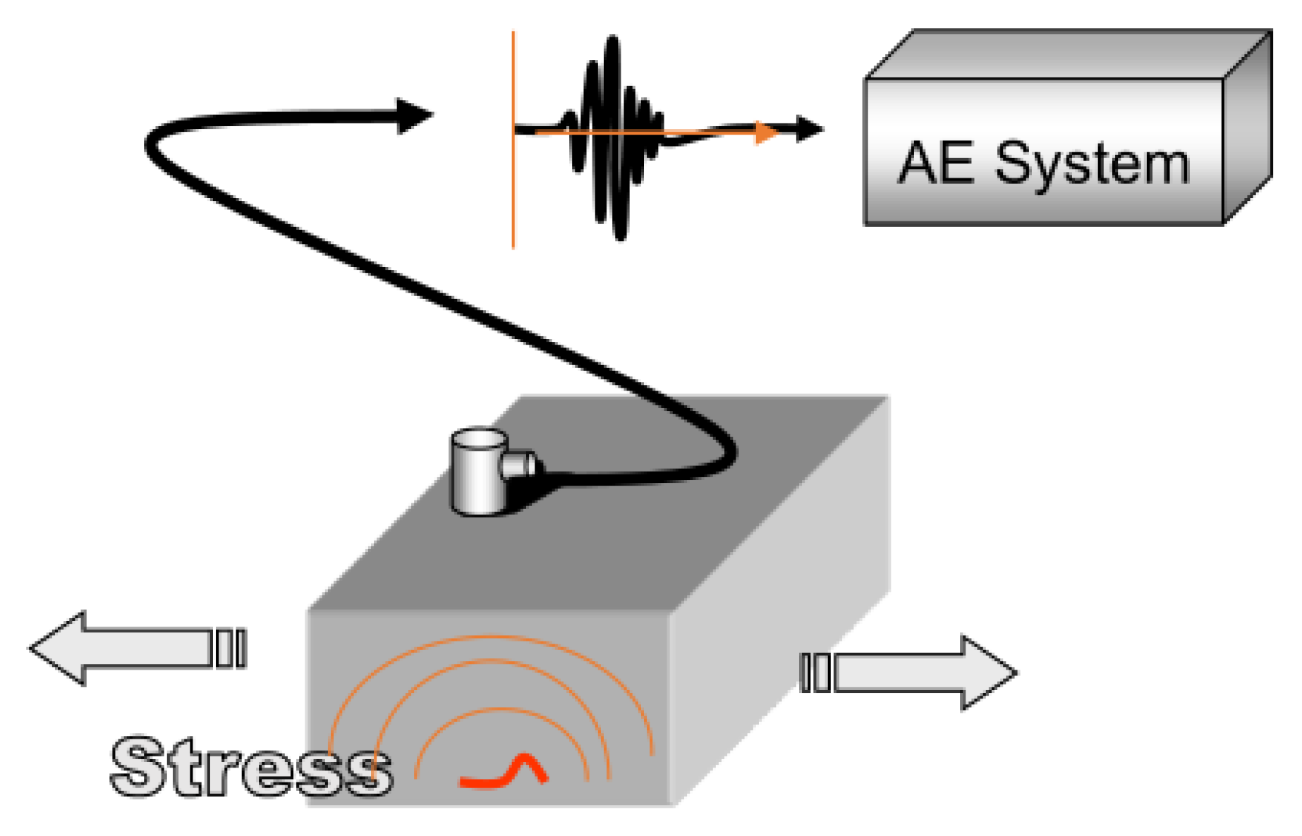
Acoustic emission (AE) technology has become one of the most effective methods for investigating damage, fracture, and their underlying mechanisms in rock masses. Acoustic emission is a phenomenon generated during the loading and deformation of rock, and the rock’s deformation and failure process can be characterized by monitoring AE parameters such as count, magnitude, and frequency. A schematic diagram of the acoustic emission test is shown in Figure 19.
For the acoustic emission (AE) experiment, rock samples were prepared and three specimens were cored at 45° increments in the horizontal plane perpendicular to the borehole core axis. The stress values at the Kaiser points along these three directions were measured, from which the maximum and minimum horizontal in situ stresses were determined. The triaxial compressive strength of rock is defined as the ultimate deviatoric stress that the rock can sustain under a three-dimensional stress state upon macroscopic failure, and is numerically equal to the maximum principal stress difference at the moment of failure.
To accurately determine the stress values corresponding to the characteristic points of the AE Kaiser effect, acoustic emission tests were conducted under different confining pressure conditions. Based on these tests, a quantitative relationship between the Kaiser point stress and the confining pressure was established (Figure 20).
σ p c = f σ 0 , P c
Under confining pressure conditions, the Kaiser point of acoustic emission is determined jointly by the AE energy and the AE ring-down count. the maximum (minimum) horizontal principal stress:
σ H = σ 0 ° + σ 90 ° 2 + σ 0 ° σ 90 ° 2 1 + tan 2 2 β 1 2 + α P p σ h = σ 0 ° + σ 90 ° 2 σ 0 ° σ 90 ° 2 1 + tan 2 2 β 1 2 + α P p
tan 2 β = σ 0 ° + σ 90 ° σ 45 ° σ 0 ° σ 90 °
The rock mass at the drill hole site exhibited minimal weathering, fully meeting the experimental requirements for in situ stress measurement. To ensure the scientific reliability of the experimental data, three depth intervals were selected from the carbonate rock strata for the verification of actual in situ stress data based on logging data. As shown in Table 1, within the carbonate rock depth range, the maximum horizontal principal stress (σH), minimum horizontal principal stress (σh), and stress increased linearly with depth in the shallow crustal layer of the Xiongan New Area and its adjacent regions (Table 2).
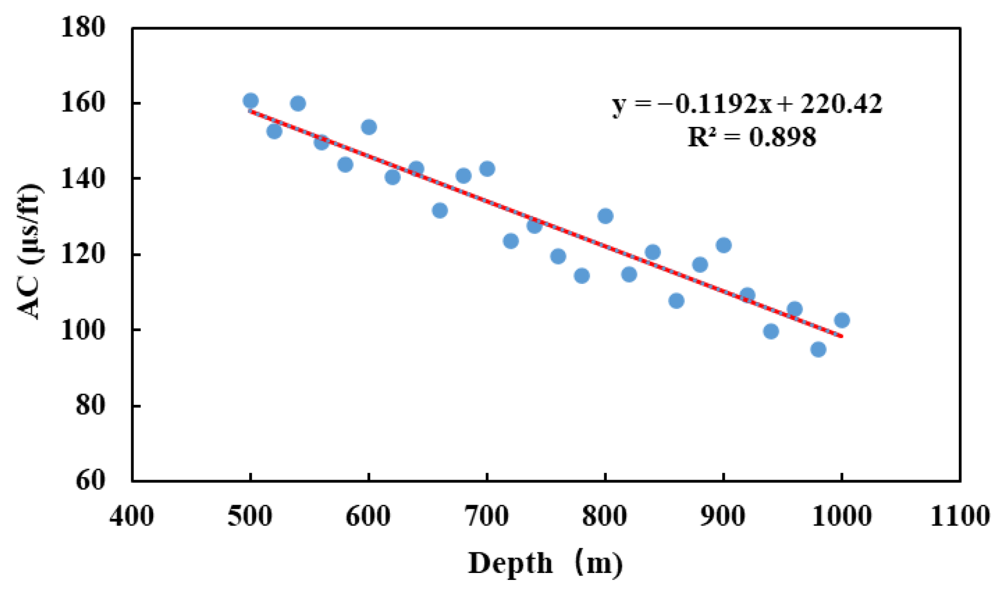
In Equation (4), ΔTn denotes the surface-fitted acoustic transit time. By fitting with Well D13, the surface acoustic transit time for the study area is obtained as 220.5 μs/ft (Figure 21).
The tectonic stress coefficient is an important parameter that quantifies the magnitude of tectonic stress acting on a region. Within the same block, the tectonic stress coefficient generally does not vary significantly with depth and can be regarded as a constant. It can be inversely determined using either core-based stress measurements or hydraulic fracturing data.
In laboratory analysis, the in situ stress magnitude is primarily measured using the differential strain method. This involves conducting three-dimensional laboratory tests on a core sample to determine the principal strains, from which the in situ principal stresses on the core are derived. When a rock sample is retrieved from the subsurface, its original stress state is destroyed, causing micro-cracks in the rock to open. The in situ stress state of the rock sample is related to the orientation and density of these opening cracks. The preferential distribution of micro-cracks induced by stress release during coring is thus a direct reflection of the in situ stress state. In core stress experiments, the process of applying confining pressure can be viewed as the reverse process of the rock’s expansion during stress release. By substituting the test results and other petrophysical parameters into a geostress calculation model, the tectonic stress coefficient can be obtained.
Alternatively, the tectonic stress coefficient can be back-calculated from hydraulic fracturing data. This requires at least two closure pressure data points. The experimentally measured maximum and minimum horizontal principal stresses are then substituted into Equation (4) to obtain the tectonic stress coefficient ε H = 0.7566 , ε h = 0.2858 .
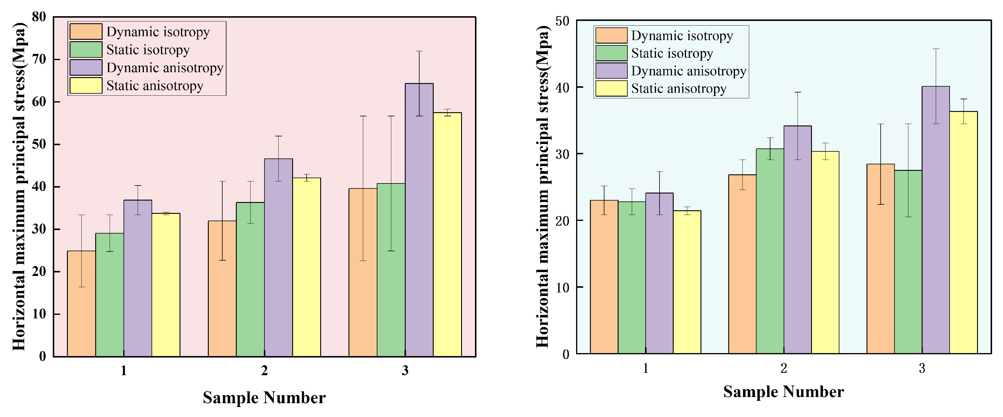
Error analysis between the modeled stress field and laboratory-measured stress magnitudes yields the following Mean Absolute Errors (MAEs). The isotropic dynamic stress model shows MAEs of 26.05% and 11.89% for the maximum and minimum horizontal principal stresses, respectively. The isotropic static stress model shows MAEs of 11.86% and 16.29%. The anisotropic dynamic stress model shows MAEs of 17.61% and 11.79%. The anisotropic static stress model shows the highest precision with MAEs of 4.14% and 3.89%, with errors controlled within 5%, meeting industrial development standards (Figure 22).
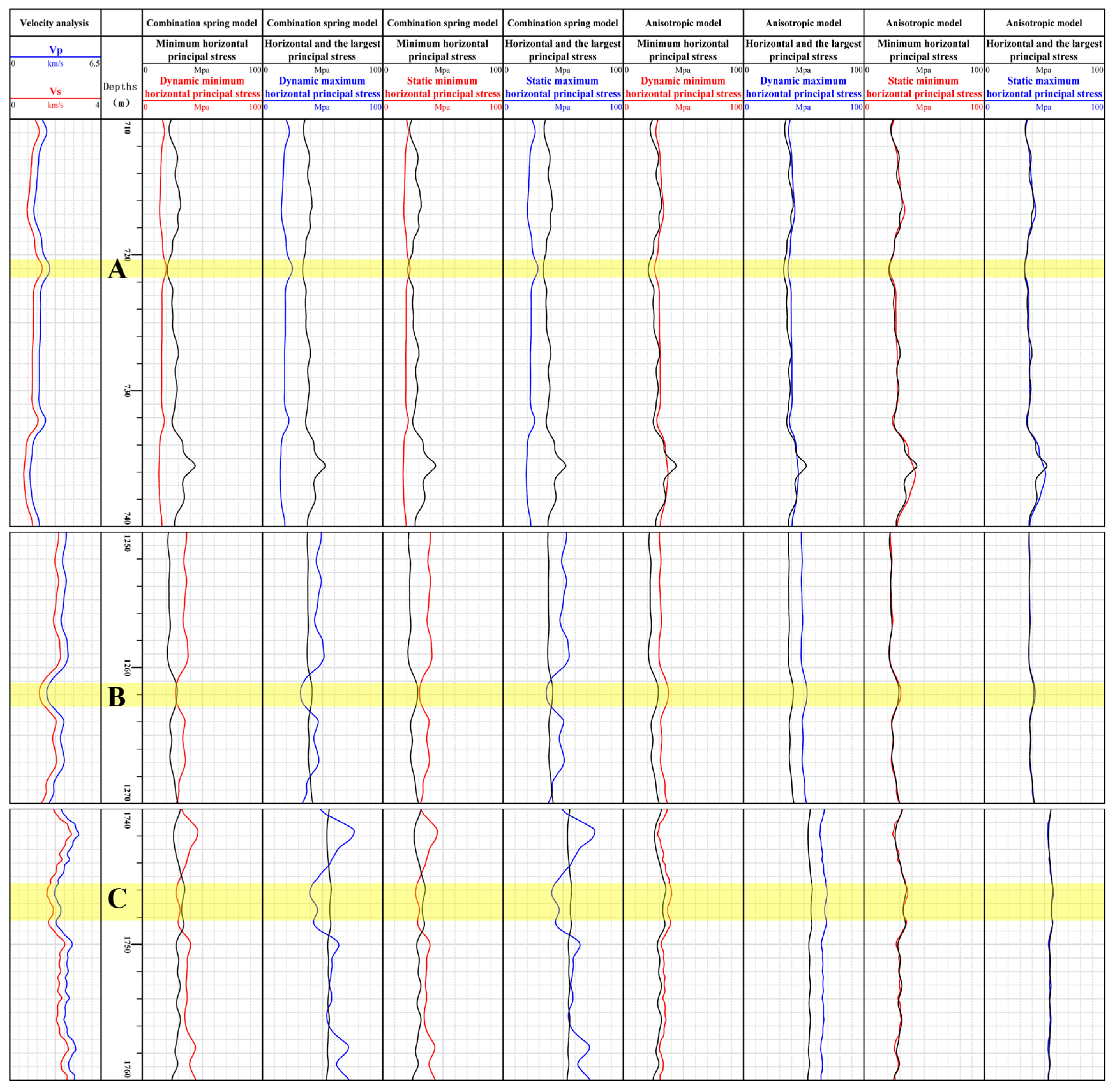
Taking Well D13 as an example, the in situ stress was evaluated by extracting the magnitude of two-dimensional in situ stress from different models. Three representative stratigraphic sections were selected: a pure mudstone stratigraphic section, a pure carbonate rock stratum, and a fault activity zone stratum. By substituting the calculated two-dimensional dynamic elastic parameters and static elastic parameters into Equations (1) and (4), respectively, various in situ stress models could be obtained. These different models were then applied to the one-dimensional in situ stress in Well D13 to compare the results and confirm whether the model outcomes were universally applicable. The specific application results are shown in Figure 23.
The stress evaluation results were highly dependent on the selected model and its input parameters. In Well D13, for the pure mudstone formation in Layer A, the results from the combined spring model (static) and the anisotropic model (static) were comparable to those from the one-dimensional model. This was because, for homogeneous, weakly isotropic sandstone, static parameter conversion is relatively reliable and anisotropic effects are not significant. The one-dimensional model provided acceptable approximations in such formations. The combined spring model using static parameters better reflected actual fracturing behavior. Layered structures introduced some anisotropy, which was captured by the anisotropic model, leading to changes in the magnitude and differences in horizontal stresses. The combined spring model, which ignored anisotropy, predicted horizontal stress differences inaccurately. One-dimensional models also failed to reflect this heterogeneity. For Layers B and C, which exhibited strong heterogeneity and (potentially) anisotropy, models considering two-dimensional characteristics (particularly anisotropy) must be employed to obtain a reliable description of the stress field. Anisotropic models could capture this effect, leading to variations in the magnitude and differences in horizontal stress.

4. Explanation of Fault Activity

The in situ stress field is primarily governed by regional tectonics and stratigraphic properties. Large faults, acting as planes of structural weakness, can cause significant disturbances in local stress fields. Theoretical and observational studies indicate that the principal stress direction near faults may undergo significant rotation: when boreholes cross faults, the horizontal maximum principal stress direction may suddenly deviate by nearly 90° [54]. Numerical simulations also confirm that the stiffness contrast of fault rupture zones is the fundamental cause of stress axis rotation. When the maximum principal stress forms a certain angle with the fault strike, the stress axes near the fault can exhibit significant torsion. Field studies have also shown that fault cores often exhibit high shear stress, while the magnitude of the maximum horizontal principal stress tends to be relatively low. Away from faults, the horizontal principal stress gradually recovers and tends toward the regional background level [55]. This indicates that faults, as weak surfaces, form stress concentrations or detachment zones around the fault contact surface, leading to abnormal phenomena such as sudden changes in stress gradients, shear stress concentration, and twists in the principal stress direction.
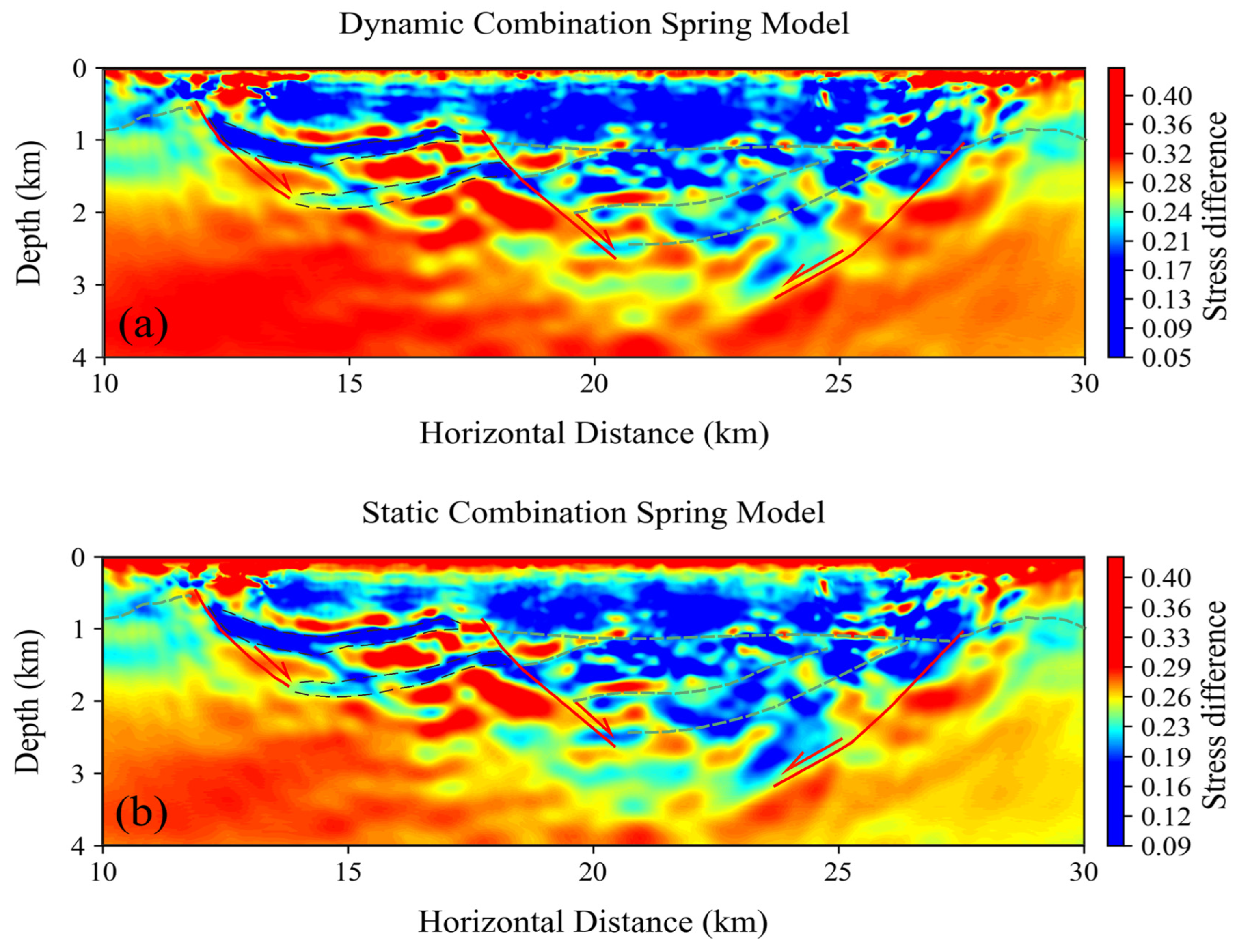
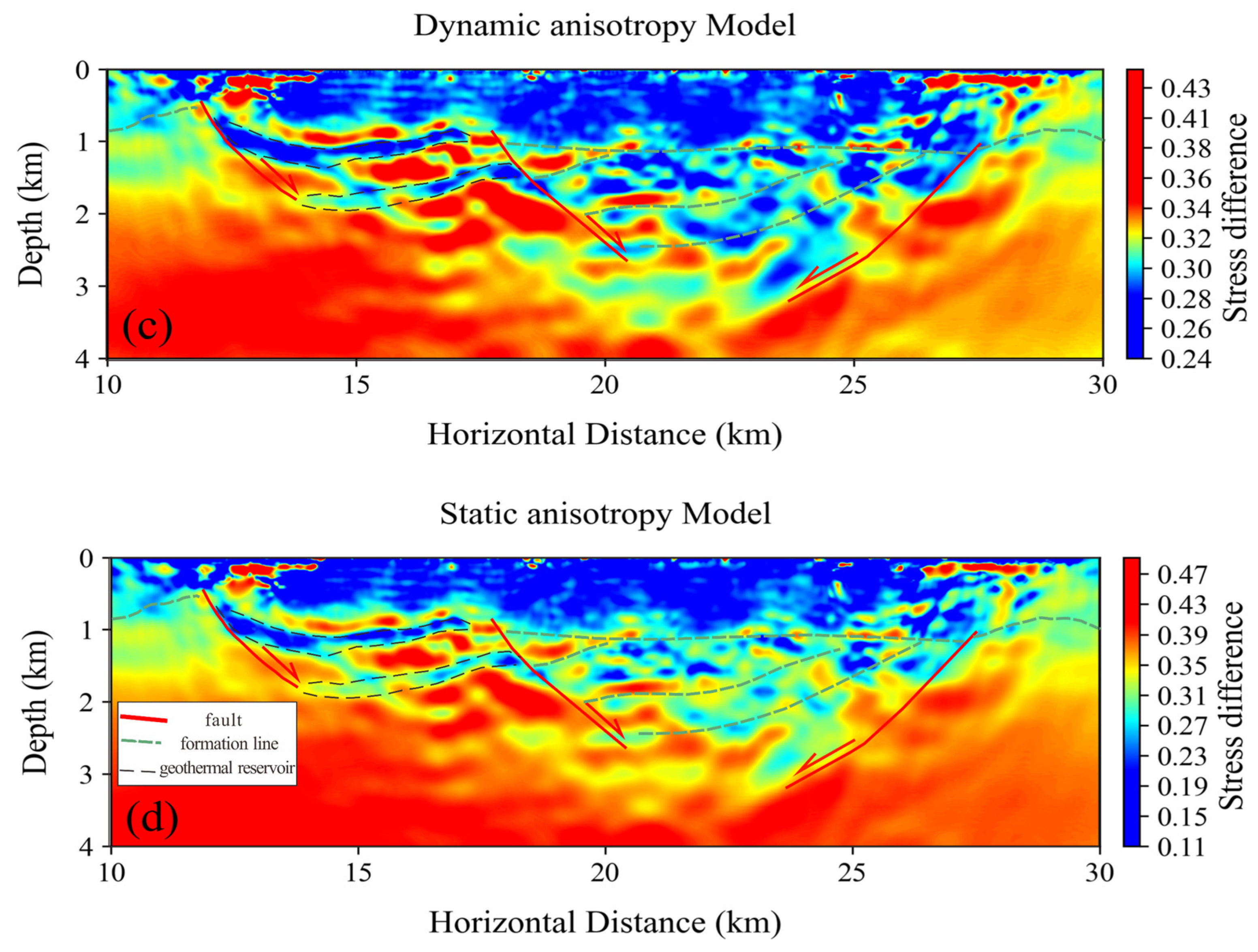
From the two-dimensional in situ stress field obtained through inversion, the direction and magnitude distribution of the horizontal principal stress are first determined, along with the stress ratio (R value) calculated from these values. Shear stress typically concentrates near faults because locked fault zones may accumulate significant shear strain energy. By screening points where shear stress exceeds the regional average, shear stress concentration zones can be identified. If a region exhibits significantly higher shear stress values, it is considered an abnormal shear stress concentration zone (as shown in Figure 24, the locations of three faults exhibit abnormal shear stress variations). High-shear stress zones often correspond to strain concentrations or potential slip surfaces and can serve as auxiliary indicators for hidden faults. For geothermal reservoirs, the first consideration is permeability assessment—the lower the minimum horizontal principal stress value, the easier it is to form natural fractures. Second, in predicting fracture direction, hydraulic fractures tend to extend perpendicular to the direction of the minimum horizontal principal stress. The black dashed lines in Figure 24 are most likely geothermal reservoirs, which have relatively high stress differences but lower stress differences near reservoir boundaries. Additionally, these geothermal reservoirs are sandwiched between two faults, meeting the criteria for geothermal reservoir formation. Finally, strike-slip faults are most likely to remain open under specific stress conditions, as shown in Figure 24d.

5. Discussion

The stress field inversion model proposed in this study establishes a mathematical formulation that integrates dynamic and static parameters with anisotropic constitutive relationships by deriving and combining them, and comprehensively accounts for the coupling mechanism between the horizontal tectonic strain field and the pore pressure field. However, the model is currently primarily applicable to stress prediction under conventional formation conditions, and there remain several aspects in terms of applicability and limitations that require further refinement.
In terms of applicability, the model demonstrates good inversion stability in lithologically relatively homogeneous intervals with clear tectonic backgrounds. Particularly in intervals where anisotropy is well-developed and well-logging and seismic data are complete, it can effectively integrate information such as P-wave velocity and shear wave splitting to achieve reliable estimation of the maximum and minimum horizontal principal stresses. By introducing a CNN–Transformer hybrid architecture, the model significantly enhances the vertical resolution and lateral continuity of velocity profiles, providing a feasible technical approach for geological blocks with moderate burial depths and good data quality.
To quantitatively assess the improvement offered by the proposed approach, we compare its performance against four representative two-dimensional in situ stress inversion methods, spanning empirical, numerical, and data-driven categories. Key characteristics and reported errors are summarized in Table 3, with detailed discussion provided below. These quantitative comparisons confirm that the proposed method offers tangible improvements over existing approaches, particularly for complex faulted reservoirs where fault-controlled stress heterogeneity is a critical factor in well placement and stimulation design.
In terms of limitations, due to the relatively shallow burial depth of the current target layer, the model does not systematically consider the coupling effects of formation temperature fields and thermal stress, which may lead to deviations in stress estimation in deep high-temperature formations or geothermally active areas. Anisotropy in subsurface media can originate from stress-induced preferential alignment of micro-fractures or from the intrinsic fabric or sedimentary structure of rock layers. Although the model can reflect the overall anisotropic characteristics, it has not yet integrated multi-attribute data such as shear wave splitting and azimuthal anisotropy to clearly distinguish the dominant mechanisms, affecting the precise interpretation of stress sources. The study area involves various lithologies, including unconsolidated sandstone and mudstone (approximately isotropic), compacted sandstone and mudstone, and carbonate rocks (significantly anisotropic). The current model shows reduced inversion accuracy at abrupt lithological changes or transitional zones between anisotropic and isotropic sections. Especially for unconsolidated intervals, applying the anisotropic model may introduce unnecessary parameter errors. Due to surface obstacles such as village distribution, local gaps exist in shallow seismic data, leading to distortions in velocity inversion and further causing systematically overestimated near-surface stress predictions, affecting the vertical continuity of the full-profile stress field.

6. Conclusions

(1)
A hybrid CNN–Transformer deep learning architecture is developed to address the cross-scale integration of seismic and well-log data. The model enhances the vertical resolution of P-wave velocity profiles from the seismic scale (20 m) to the well-log scale (0.1 m) with a prediction accuracy of 95% (R2 = 0.9671, MSE = 0.0215). By incorporating high-frequency well-log information while preserving the lateral continuity inherent in seismic data, this approach provides refined velocity inputs for geomechanical modeling and establishes a novel technical pathway for high-resolution fault characterization.
(2)
A two-dimensional in situ stress inversion workflow jointly constrained by well logs and seismic data is established for integrated fault activity interpretation. By combining dynamic and static mechanical parameters with a combined spring model and a VTI anisotropic constitutive model, the workflow explicitly accounts for stress-field anisotropy. Quantitative error analysis against laboratory-measured stress magnitudes (AE Kaiser effect) yields mean absolute errors for the anisotropic static model of 4.14% (σH) and 3.89% (σh), both controlled within 5% and meeting industrial development standards. The workflow demonstrates significant advantages in computational efficiency, lateral continuity, and vertical resolution compared with conventional single-scale inversion approaches.
(3)
Comparative analysis of four stress models reveals that the anisotropic static model achieves the highest precision, with error reductions of approximately 65–75% relative to isotropic models (MAE: 26.05% and 11.89% for the isotropic dynamic model; 11.86% and 16.29% for the isotropic static model). The results confirm that explicit incorporation of formation anisotropy and static elastic parameters is essential for reliable stress prediction in heterogeneous, faulted carbonate sequences. The proposed framework enables coupled stress–fault analysis and provides a high-precision geophysical basis for crustal stability assessment and hydraulic fracturing design in complex structural zones.

Author Contributions

K.W.: Conceptualization, Data curation, Formal analysis, Funding acquisition, Writing—review and editing. X.N.: Writing—original draft, Investigation, Methodology, Data curation, Visualization. X.W.: Software, Investigation, Validation methodology, Visualization, Writing—review and editing. F.W.: Funding acquisition, Investigation, Methodology. J.L.: Funding acquisition, Formal analysis, Supervision. T.W.: Data curation, Validation, Investigation. F.Y.: Investigation, Formal analysis, Project administration. All authors have read and agreed to the published version of the manuscript.

Funding

This work is supported by Deep Earth probe and Mineral Resources Exploration-National Science and Technology Major Project (grant no. 2024ZD1002305) and the China Geological Survey Project (grant no. DD20230298) and Shaanxi Province Natural Science Basic Research Program “Research on Evaluation Method for Fracability of Shale Gas Reservoirs Based on Volume Fracturing” (grant no. 2025JC-YBMS-312).

Data Availability Statement

The datasets presented in this article are not readily available because of data confidentiality restrictions. The raw well logging data and seismic profile data supporting the findings of this study are confidential and cannot be shared publicly. Requests for access to the datasets or further information may be directed to the corresponding author, Wang Xiaojiang, upon reasonable request.

Conflicts of Interest

Authors Kai Wang, Xiaojiang Wang, Jianxun Liu, Tong Wang was employed by Institute of Geophysical and Geochemical Exploration, CAGS, Tianjin, 300300, The National Center of Geological Exploration Technology, Tianjin, 300300 and State Key Laboratory of Deep Earth Exploration and Imaging, Institute of Geophysical and Geochemical Exploration, Chinese Academy of Geological Sciences, Tianjin, 300300; Author Fan Yong was employed by Institute of Geophysical and Geochemical Exploration, CAGS, Tianjin, 300300 and The National Center of Geological Exploration Technology, Tianjin, 300300. The authors declare no conflicts of interest.

References

  1. Kruszewski, M. The In Situ Stress State, Its Variability, and Implications for Conventional and Unconventional Geothermal Reservoirs. Ph.D. Thesis, Ruhr-Universität Bochum, Bochum, Germany, 2023. [Google Scholar]
  2. Tomac, I.; Sauter, M. A review on challenges in the assessment of geomechanical rock performance for deep geothermal reservoir development. Renew. Sustain. Energy Rev. 2018, 82, 3972–3980. [Google Scholar] [CrossRef]
  3. Zhang, F.; Damjanac, B.; Maxwell, S. Investigating Hydraulic Fracturing Complexity in Naturally Fractured Rock Masses Using Fully Coupled Multiscale Numerical Modeling. Rock Mech. Rock Eng. 2019, 52, 5137–5160. [Google Scholar] [CrossRef]
  4. Zu, K.; Wang, Z.; Wang, S.; Zhou, S.; Jiang, Y.; Li, Z. A new approach for quantitative evaluating natural fracture effectiveness in tight carbonate reservoir. J. Appl. Geophys. 2025, 241, 105814. [Google Scholar] [CrossRef]
  5. Sun, H.; Tian, S.; Xiang, Y.; Cheng, L.; Yang, F. Analysis of Stress Perturbation Patterns in Oil and Gas Reservoirs Induced by Faults. Processes 2025, 13, 1416. [Google Scholar] [CrossRef]
  6. He, K.; Yuan, Y.; Sheng, Y.; Li, H. Integrated Geophysical Hydrogeological Characterization of Fault Systems in Sandstone-Hosted Uranium In Situ Leaching: A Case Study of the K1b2 Ore Horizon, Bayin Gobi Basin. Processes 2025, 13, 3313. [Google Scholar] [CrossRef]
  7. Yang, S.; Li, X.; Wang, K.; Ping, G. Developmental Characteristics of Post-Rift Faults and Palostress Field Inversion in the Bozhong 19-6 Structural Belt. Processes 2025, 13, 2726. [Google Scholar] [CrossRef]
  8. Özdemir, H. Seismic Amplitude Versus Offset Analysis and Amplitude Inversion Theory and Practice—A Comprehensive Review: Volume 1—Preliminaries of Seismic Inversion, and AVO Analysis; Springer Nature: Cham, Switzerland, 2026. [Google Scholar]
  9. Wang, H.; Liao, X.; Ding, H. Monitoring and evaluating the volume fracturing effect of horizontal well. J. Nat. Gas Sci. Eng. 2015, 22, 498–502. [Google Scholar] [CrossRef]
  10. Wei, X.; Yang, Z.; Yan, X. Multi-scale issue in seismic exploration and its research progress. Prog. Geophys. 2019, 34, 2353–2360. [Google Scholar] [CrossRef]
  11. Zhang, M.; Wang, Y.; Feng, Q.; Luo, Y.; Yu, Z. Constrained spatial structure reconstruction for low-frequency model building in seismic inversion. Geophys. Prospect. Pet. 2025, 65, 40–54. [Google Scholar] [CrossRef]
  12. Contreras, A.; Torres-Verdín, C.; Chesters, W.; Kvien, K.; Fasnacht, T. Joint stochastic inversion of 3D pre-stack seismic data and well logs for high-resolution reservoir characterization and petrophysical modeling: Application to deepwater hydrocarbon reservoirs in the central Gulf of Mexico. In SEG Technical Program Expanded Abstracts; GeoScienceWorld: Washington, DC, USA, 2005; pp. 1343–1346. [Google Scholar]
  13. Yin, S.; Zhang, J.; Deng, H.; Qin, H.; Xia, W.; Du, Y.; Gong, M.; Huang, T.; Li, C. Evaluation methods and engineering applications of in-situ stress in deep, strong heterogeneity terrestrial shale oil and gas reservoirs: A case study of jurassic shales in the Yingshan-Pingchang area, northeast Sichuan. Front. Earth Sci. 2025, 13, 1530002. [Google Scholar] [CrossRef]
  14. Ge, X.; Guo, T.; Li, M.; Zhao, P.; Deng, H.; Li, W.; Zhong, C. Evaluation and optimization of “engineering sweet spot” in deep shale reservoir: Case study on Yongchuan and Dingshan areas in southern Sichuan. Exp. Pet. Geol. 2023, 45, 210–221. [Google Scholar] [CrossRef]
  15. Fang, X.; Wang, Y.; Zhang, Y.; Li, F. Rock mechanical properties and fracability evaluation of deep tight hybrid sedimentary rocks reservoirs-a case study of Lucaogou formation in Jimsar Sag, Junggar Basin. J. Pet. Explor. Prod. Technol. 2025, 15, 67. [Google Scholar] [CrossRef]
  16. Dou, L.; Zuo, X.; Qu, L.; Xiao, Y.; Bi, G.; Wang, R.; Zhang, M. A New Method of Quantitatively Evaluating Fracability of Tight Sandstone Reservoirs Using Geomechanics Characteristics and In Situ Stress Field. Processes 2022, 10, 1040. [Google Scholar] [CrossRef]
  17. Zhu, S.; Zhang, Y.; Zha, B.; Cao, X.; Pu, L.; Huang, C. Prediction of In Situ Stress in Ultra-Deep Carbonate Reservoirs Along Fault Zone 6 of the Shunbei Ordovician System Based on a Two-Parameter Coupling Model with Nonlinear Perturbations. Processes 2025, 13, 3822. [Google Scholar] [CrossRef]
  18. Yang, H.; Li, Z.; Yang, H.; Wang, Y.; Hui, C.; Guo, Y. Analysis of Fault Influence on Geostress Perturbation Based on Fault Model Test. Processes 2024, 12, 1240. [Google Scholar] [CrossRef]
  19. Benayad, S.; Sen, S.; Baouche, R.; Chaouchi, R. In-situ stress state and critically stressed fracture analysis from the Hassi D’Zabat field, Algeria—A study from the naturally fractured Cambro-Ordovician reservoirs. J. Appl. Geophys. 2025, 233, 105630. [Google Scholar] [CrossRef]
  20. Ervine, W.B.; Bell, J.S. Subsurface in situ stress magnitudes from oil-well drilling records: An example from the Venture area, offshore eastern Canada. Can. J. Earth Sci. 1987, 24, 1748–1759. [Google Scholar] [CrossRef]
  21. Bedell, J.; Ismail, A.; Grammer, M.; Puckette, J.; Mewafy, F.; Boykin, B. Multiscale fractures, stress and reservoir quality characterization: The Mississippian Meramec and Osage intervals, STACK play, Central Oklahoma. J. Appl. Geophys. 2023, 219, 105244. [Google Scholar] [CrossRef]
  22. Matthews, W.R.; Kelly, J. How to Predict Formation Pressure and Fracture Gradient from Electric and Sonic Logs. Oil Gas 1967, 20, 92–106. [Google Scholar]
  23. Anderson, R.A.; Ingram, D.S.; Zanier, A.M. Determining Fracture Pressure Gradients from Well Logs. J. Pet. Technol. 1973, 25, 1259–1268. [Google Scholar] [CrossRef]
  24. Daines, S.R. Prediction of Fracture Pressures for Wildcat Wells. J. Pet. Technol. 1982, 34, 863–872. [Google Scholar] [CrossRef]
  25. Newberry, B.M.; Nelson, R.F.; Ahmed, U. Prediction of Vertical Hydraulic Fracture Migration Using Compressional and Shear Wave Slowness. In Proceedings of the SPE Low Permeability Gas Reservoirs Symposium, Denver, CO, USA, 19–22 May 1985. [Google Scholar]
  26. Huang, R.; Zhuang, J. A new method for predicting formation fracture pressure. Oil Drill. Process 1986, 3, 1–14. [Google Scholar] [CrossRef]
  27. Thiercelin, M.J.; Plumb, R.A. Core-Based Prediction of Lithologic Stress Contrasts in East Texas Formations. SPE Form. Eval. 1994, 9, 251–258. [Google Scholar] [CrossRef]
  28. Higgins, S.; Goodwin, S.; Donald, A.; Bratton, T.; Tracy, G. Anisotropic Stress Models Improve Completion Design in the Baxter Shale. In Proceedings of the SPE Annual Technical Conference and Exhibition, Denver, CO, USA, 21–24 September 2008. [Google Scholar]
  29. Cruz, L.; Jimba, S.; Affinito, R.; Husain, Z. Stress Variations Controlled by Rock Composition in an Appraisal Well in the US: Evaluating Lithology, Stress Measurements, and Methods. In Proceedings of the 58th U.S. Rock Mechanics/Geomechanics Symposium, Golden, CO, USA, 23–26 June 2024; OnePetro: Richardson, TX, USA, 2024. [Google Scholar]
  30. Wojtowicz, M.; Jarosinski, M. Reconstructing the mechanical parameters of a transversely-isotropic rock based on log and incomplete core data integration. Int. J. Rock Mech. Min. Sci. 2019, 115, 111–120. [Google Scholar] [CrossRef]
  31. Bian, H.; Wang, F.; Zhang, C.; Gao, X.; Zhang, Y.; Duan, C.; Li, D. A New Model between Dynamic and Static Elastic Parameters of Shale Based on Experimental Studies. Arab. J. Geosci. 2019, 12, 609. [Google Scholar] [CrossRef]
  32. Fjaer, E. Relations between static and dynamic moduli of sedimentary rocks. Geophys. Prospect. 2019, 67, 128–139. [Google Scholar] [CrossRef]
  33. Khosravi, M.; Tabasi, S.; Eldien, H.H.; Motahari, M.R.; Alizadeh, S.M. Evaluation and prediction of the rock static and dynamic parameters. J. Appl. Geophys. 2022, 199, 104581. [Google Scholar] [CrossRef]
  34. Nejati, M.; Dambly, M.L.T.; Saar, M.O. A methodology to determine the elastic properties of anisotropic rocks from a single uniaxial compression test. J. Rock Mech. Geotech. Eng. 2019, 11, 1166–1183. [Google Scholar] [CrossRef]
  35. Krietsch, H.; Gischig, V.; Evans, K.; Doetsch, J.; Dutler, N.O.; Valley, B.; Amann, F. Stress Measurements for an In Situ Stimulation Experiment in Crystalline Rock: Integration of Induced Seismicity, Stress Relief and Hydraulic Methods. Rock Mech. Rock Eng. 2019, 52, 517–542. [Google Scholar] [CrossRef]
  36. Melendez-Martinez, J.; Schmitt, D.R. A comparative study of the anisotropic dynamic and static elastic moduli of unconventional reservoir shales: Implication for geomechanical investigations. Geophysics 2016, 81, D245–D261. [Google Scholar] [CrossRef]
  37. Ghasemi, M.F.; Bayuk, I.O. Application of rock physics modelling to investigate the differences between static and dynamic elastic moduli of carbonates. Geophys. J. Int. 2020, 222, 1992–2023. [Google Scholar] [CrossRef]
  38. Suo, Y.; Su, X.; Wang, Z.; He, W.; Fu, X.; Feng, F.; Pan, Z.; Xie, K.; Wang, G. A study of inter-stratum propagation of hydraulic fracture of sandstone-shale interbedded shale oil. Eng. Fract. Mech. 2022, 275, 108858. [Google Scholar] [CrossRef]
  39. Cao, H.; Zhao, Y.; Shuai, D.; Qi, Y.; Chen, G.; Li, S. Using 3D seismic data to estimate stress based on seismic curvature attribute of HTI medium: Application to the Weiyuan, southern Sichuan Basin, China. Chin. J. Geophys. 2024, 67, 1970–1986. (In Chinese) [Google Scholar] [CrossRef]
  40. Eaton, B.A. Fracture Gradient Prediction and Its Application in Oilfield Operations. J. Pet. Technol. 1969, 21, 1353–1360. [Google Scholar] [CrossRef]
  41. Liu, W.; Wang, Y.; Chen, Z.; Chen, C.; Shen, H.; Zhang, F.; Zhang, T. Anisotropic dynamic-static elastic parameter correlations for Jurassic lacustrine shales. Chin. J. Geophys. 2025, 68, 213–228. [Google Scholar] [CrossRef]
  42. Ohno, I.; Abe, M.; Kimura, M.; Hanayama, Y.; Oda, H.; Suzuki, I. Elasticity measurement of silica glass under gas pressure. Am. Mineral. 2000, 85, 288–291. [Google Scholar] [CrossRef]
  43. Horsrud, P.; SØnstebØ, E.F.; BØe, R. Mechanical and petrophysical properties of North Sea shales. Int. J. Rock Mech. Min. Sci. 1998, 35, 1009–1020. [Google Scholar] [CrossRef]
  44. Shapiro, S.A. Elastic piezosensitivity of porous and fractured rocks. Geophysics 2002, 68, 482–486. [Google Scholar] [CrossRef]
  45. Mah, M., Jr.; Schmitt, D.R., Jr. Experimental determination of the elastic coefficients of an orthorhombic material. Geophysics 2001, 66, 1217–1225. [Google Scholar] [CrossRef]
  46. Wang, F.; Nie, X.; Zhang, D.; Guo, Y.; Bian, H. Shale In-Situ Stress logging prediction method based on dynamic, static and anisotropic. Chin. J. Geophys. 2026, 69, 411–425. (In Chinese) [Google Scholar]
  47. He, D.; Shan, S.; Zhang, Y.; Lu, R.; Zhang, R.; Cui, Y. 3-D geologic architecture of Xiong’an New Area: Constraints from seismic reflection data. Sci. China Earth Sci. 2018, 61, 1007–1022. [Google Scholar] [CrossRef]
  48. Wang, K.; Feng, X.; Malcolm, A.; Williams, C.; Wang, X.; Zhang, K.; Zhang, B.; Yue, H. Multiscale Full-Waveform Inversion with Land Seismic Field Data: A Case Study from the Jizhong Depression, Middle Eastern China. Energies 2022, 15, 3223. [Google Scholar] [CrossRef]
  49. He, Z.; Shao, H.; Zhong, X.; Zhao, X. Ensemble transfer CNNs driven by multi-channel signals for fault diagnosis of rotating machinery cross working conditions. Knowl.-Based Syst. 2020, 207, 106396. [Google Scholar] [CrossRef]
  50. Agga, A.; Abbou, A.; Labbadi, M.; Houm, Y.E.; Ou Ali, I.H. CNN-LSTM: An efficient hybrid deep learning architecture for predicting short-term photovoltaic power production. Electr. Power Syst. Res. 2022, 208, 107908. [Google Scholar] [CrossRef]
  51. Vaswani, A.; Shazeer, N.; Parmar, N.; Uszkoreit, J.; Jones, L.; Gomez, A.N.; Kaiser, Ł.; Polosukhin, I. Attention is all you need. In Proceedings of the 31st International Conference on Neural Information Processing Systems, Long Beach, CA, USA, 4–9 December 2017; Curran Associates Inc.: Red Hook, NY, USA, 2017; pp. 6000–6010. [Google Scholar]
  52. Wang, Y.; Zhao, L.; Han, D.-H.; Wei, Q.; Zhang, Y.; Yuan, H.; Geng, J. Experimental quantification of the evolution of the static mechanical properties of tight sedimentary rocks during increasing-amplitude load and unload cycling. Geophysics 2022, 87, MR73–MR83. [Google Scholar] [CrossRef]
  53. Han, P.; Ding, W.; Ma, H.; Yang, D.; Lv, J.; Li, Y.; Liu, T. The method and application of numerical simulation of high-precision stress field and quantitative prediction of multiperiod fracture in carbonate reservoir. Tectonophysics 2024, 885, 230421. [Google Scholar] [CrossRef]
  54. Ziegler, M.O.; Seithel, R.; Niederhuber, T.; Heidbach, O.; Kohl, T.; Müller, B.; Rajabi, M.; Reiter, K.; Röckel, L. Stress state at faults: The influence of rock stiffness contrast, stress orientation, and ratio. Solid Earth 2024, 15, 1047–1063. [Google Scholar] [CrossRef]
  55. Yuan, D.; Zhang, L.; Liu, X.; Feng, T.; Zhang, G.; Xu, Z.; Wang, Z.; Yi, X.; Lin, Z.; Ren, Y.; et al. Influence of the Xianshuihe Fault Zone on In-Situ Stress Field of a Deep Tunnel and its Engineering Effect. Front. Earth Sci. 2022, 10, 886876. [Google Scholar] [CrossRef]
  56. Ma, N.; Yin, X.Y.; Sun, C.Y.; Zong, Z.Y. The in-situ stress seismic prediction method based on the theory of orthorhombic anisotropic media. Chin. J. Geophys. 2017, 60, 4766–4775. [Google Scholar] [CrossRef]
  57. Lee, H.; Ong, S.H. Estimation of In Situ Stresses with Hydro-Fracturing Tests and a Statistical Method. Rock Mech. Rock Eng. 2018, 51, 779–799. [Google Scholar] [CrossRef]
  58. Li, X.; Zhou, X.; Xu, Z.; Feng, T.; Wang, D.; Deng, J.; Zhang, G.; Li, C.; Feng, G.; Zhang, R.; et al. Inversion Method of Initial In Situ Stress Field Based on BP Neural Network and Applying Loads to Unit Body. Adv. Civ. Eng. 2020, 2020, 8840940. [Google Scholar] [CrossRef]
  59. Liu, X.; Huang, C.; Zhu, W.; Oh, J.; Zhang, C.; Si, G. In situ stress inversion using nonlinear stress boundaries achieved by the bubbling method. J. Rock Mech. Geotech. Eng. 2025, 17, 1510–1527. [Google Scholar] [CrossRef]
Figure 1. Technology roadmap.
Processes 14 01567 g001
Figure 3. Two-dimensional velocity profile. (a) Restored model overlaid on the seismic profile; (b) geological interpretation of the restored model [48].
Processes 14 01567 g003
Figure 4. Local P-wave velocity profile containing well locations.
Processes 14 01567 g004
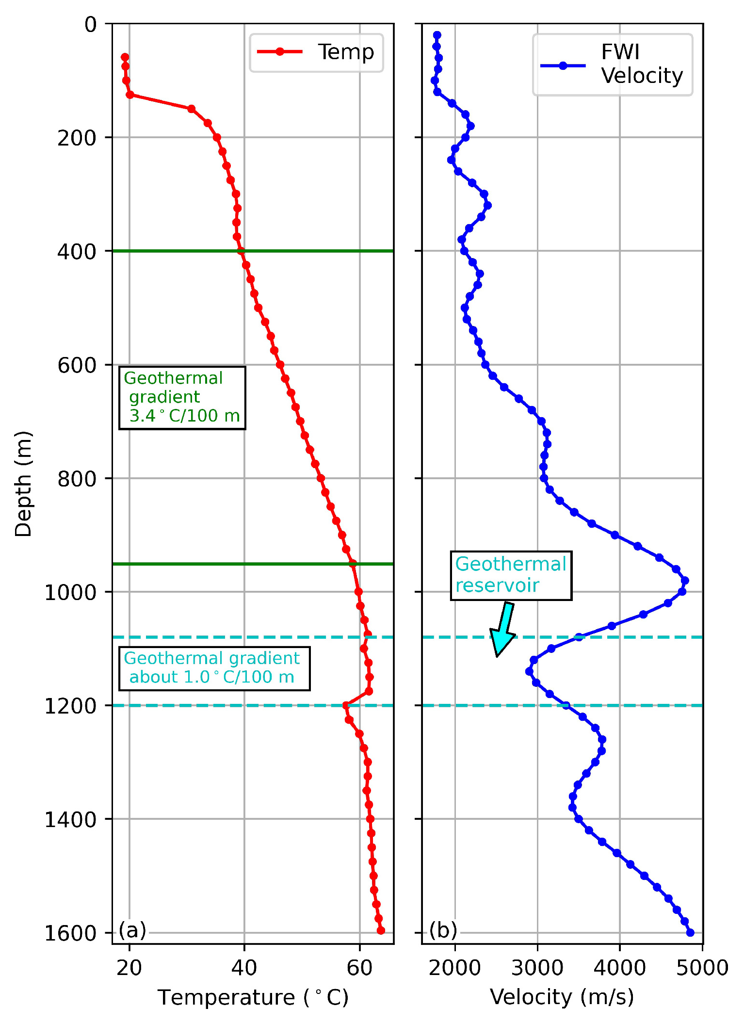
Figure 5. The relationship between stratum temperature and velocity. The temperature data come from well D13. (a) The stratum temperature increases as a function of depth. (b) There is a low-velocity anomaly in the same depth range between 1100 m and 1200 m.
Processes 14 01567 g005
Figure 6. Comparison of Model-Fitted P-Wave Velocity with Logged P-Wave Velocity and P-Wave Velocity Inferred from Seismic Data.
Processes 14 01567 g006
Figure 7. Schematic of a CNN architecture.
Processes 14 01567 g007
Figure 8. Schematic of the Transformer network architecture.
Processes 14 01567 g008
Figure 9. Neural network structure framework diagram.
Processes 14 01567 g009
Figure 10. Model Evaluation Metrics. (a) True Values Vs. Predicted Values; (b) Error Distribution Histogram; (c) True and Predicted Values Vs. Depth.
Processes 14 01567 g010
Figure 11. High-precision velocity and density profiles. (a) Shear wave velocity profile; (b) density profile.
Processes 14 01567 g011
Figure 12. Flow chart of the principle of acoustic-mechanical co-testing of rock samples.
Processes 14 01567 g012
Figure 13. Calculation of static elastic mechanical parameters.
Processes 14 01567 g013
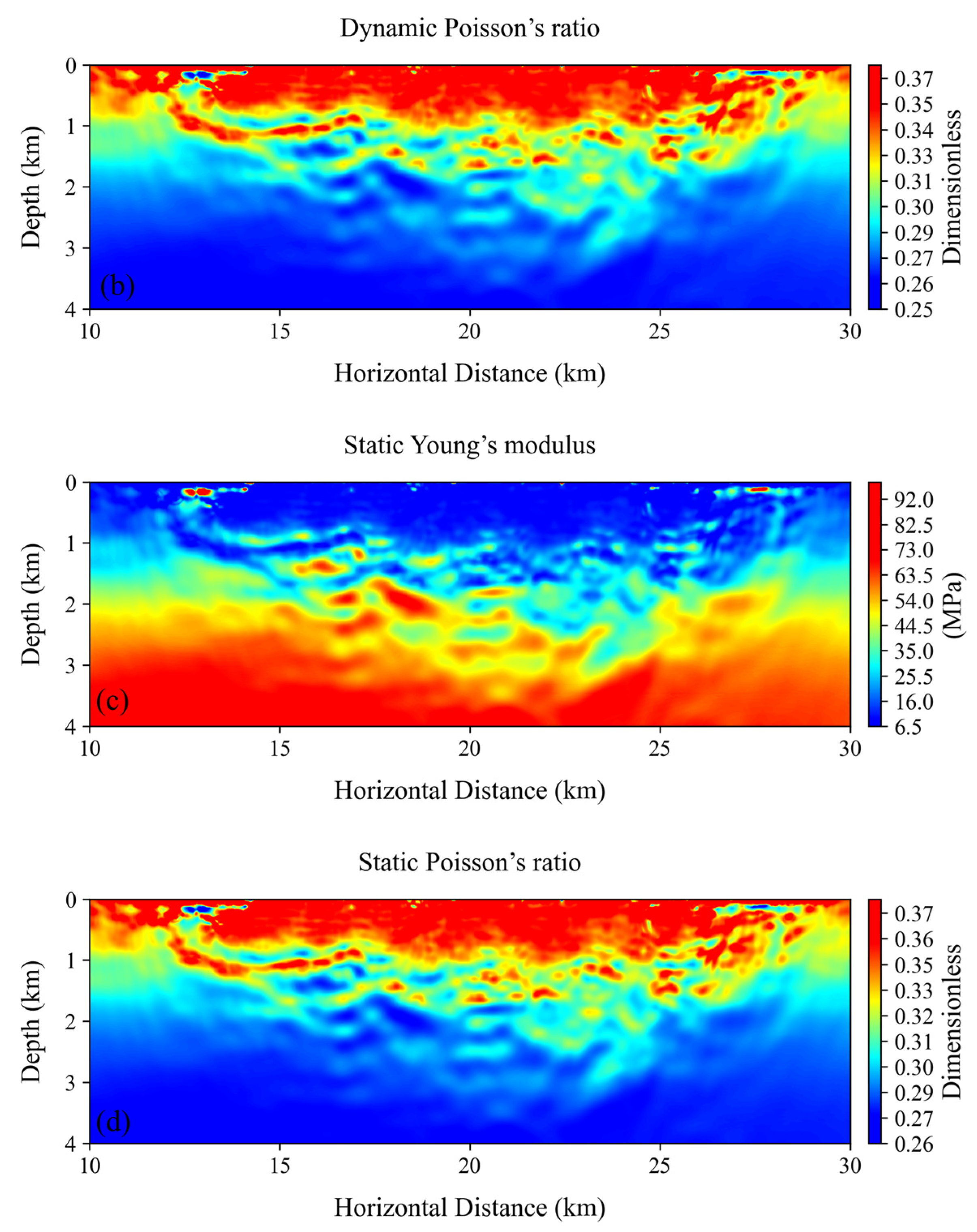
Figure 14. Dynamic and static elasticity parameter profiles. (a) Dynamic Young’s modulus profile; (b) dynamic Poisson’s ratio profile; (c) static Young’s modulus profile; (d) static Poisson’s ratio profile.
Processes 14 01567 g014aProcesses 14 01567 g014b
Figure 15. Monte Carlo Uncertainty Analysis of Static Young’s Modulus.
Processes 14 01567 g015
Figure 16. Two-dimensional stress profiles. (a,b) Horizontal (a) maximum and (b) minimum principal stress profiles of the dynamic combined spring model. (c,d) Horizontal (c) maximum and (d) minimum principal stress profiles of the static combined spring model.
Processes 14 01567 g016
Figure 17. Two-dimensional stress profiles. (a,b) Horizontal (a) maximum and (b) minimum principal stress profiles of the dynamic anisotropic model. (c,d) Horizontal (c) maximum and (d) minimum principal stress profiles of the static anisotropic model.
Processes 14 01567 g017
Figure 18. Intersection of static stiffness coefficients in the laboratory. (a) Crossplot of stiffness coefficients C66s vs. C11a; (b) Crossplot of stiffness coefficients C11s vs. C11a; (c) Crossplot of stiffness coefficients C33s vs. C13a; (d) Crossplot of stiffness coefficients C44s vs. C11s; (e) Crossplot of model-predicted C12s vs. measured C12s; (f) Crossplot of model-predicted C13s vs. measured C13s.
Processes 14 01567 g018
Figure 19. Schematic diagram of the acoustic emission testing system.
Processes 14 01567 g019
Figure 20. AE activity frequency versus applied stress at 1746.4 m depth, Well D13.
Processes 14 01567 g020
Figure 21. Fitting relationship between acoustic transit time and depth for Well D13.
Processes 14 01567 g021
Figure 22. Error Analysis of in situ stress.
Processes 14 01567 g022
Figure 23. Comparison between one-dimensional logging-based in situ stress and different two-dimensional in situ stress models in Well D13. (a) Layer A: Homogeneous mudstone with weak anisotropy. (b) Layer B: Shallow heterogeneous formation with strong anisotropy. (c) Layer C: Deep heterogeneous formation with strong anisotropy.
Processes 14 01567 g023
Figure 24. Fault identification using the stress ratio method with different in situ stress models. (a) Fault identification by stress difference: dynamic combined spring model. (b) Fault identification by stress difference: static combined spring model. (c) Fault identification by stress difference: dynamic anisotropic model. (d) Fault identification by stress difference: static anisotropic model.
Processes 14 01567 g024aProcesses 14 01567 g024b
Table 1. Model Parameter Optimization Results.
HierarchyParameterSearch RangeOptimal Result
Network
Architecture
Encoder Channels[32, 64, 128][64, 128, 256]
Encoder Kernel Size[3, 5, 7][7, 5, 3]
Number of Transformer Heads[4, 8, 12]8
Number of Transformer Encoder Layers[2, 4, 6]4
Number of Transformer Decoder Layers[2, 4, 6]4
Feedforward Network Dimension[256, 512, 1024]512
Decoder Channels[32, 64, 128][128, 64, 1]
Decoder Kernel Size[3, 5, 7][5, 3, 1]
Training
Optimization
Training Epochs[50, 100, 200]100
Batch Size (GPU)[8, 16, 32]16
Batch Size (CPU)[4, 8, 16]8
Initial Learning Rate[0.00001, 0.0001, 0.001]0.0001
Loss Function[MSE, MAE, Huber]MSE
Table 2. Core-based in situ stress test results for Well D13.
SharpDepths (m)σH (MPa)σh (MPa)Horizontal Stress Difference MPa
D13721.033.3920.8212.57
1261.5541.2629.0612.20
1746.456.6734.4622.21
Table 3. Quantitative comparison of representative 2D in situ stress inversion methods.
Method CategoryData SourceModeling FrameworkReported Error (σH/σh)
Seismic curvature attribute [56]Post-stack seismicEmpirical attribute mappingQualitative; no stress-magnitude
error reported
FEM geomechanical simulation (linear elastic) [57]Log + regional tectonic BC2D plane-strain FEM with linear elastic constitutive modelRMSE ≈ 4.15–5.0 MPa; relative error ≈ 16–22%
BP neural network (unit-body loading) [58]Log + tectonic strainData-driven ML (BP-NN)Average relative error:
σH 12.24%, σh 13.22%
Nonlinear FEM (bubbling method) [59]Log + in situ stress measurementsNonlinear FEM inversionRMSE 3.2;
relative error 17.55%
This study (well-seismic integrated FWI + CNN–Transformer)Multisource (well log + seismic FWI + fault interpretation)2D stress inversion with combined spring + anisotropic model; CNN–Transformer for log-seismic fusionMean absolute error:
σH 4.14%, σh 3.89%
Disclaimer/Publisher’s Note: The statements, opinions and data contained in all publications are solely those of the individual author(s) and contributor(s) and not of MDPI and/or the editor(s). MDPI and/or the editor(s) disclaim responsibility for any injury to people or property resulting from any ideas, methods, instructions or products referred to in the content.