Article

Fast Risk Assessment for Receiving-End Power Grids with High Penetration of Renewable Energy Based on the Fault Transient Evolution Process

1
Key Laboratory of Power System Intelligent Dispatch and Control of Ministry of Education, Shandong University, Jinan 250061, China
2
State Grid Shandong Electric Power Research Institute, Jinan 250003, China
*
Author to whom correspondence should be addressed.
Processes 2026, 14(1), 120; https://doi.org/10.3390/pr14010120 (registering DOI)
Submission received: 28 November 2025 / Revised: 21 December 2025 / Accepted: 26 December 2025 / Published: 29 December 2025
(This article belongs to the Special Issue Modeling, Operation and Control in Renewable Energy Systems)

Abstract

Addressing the complexity of transient evolution and the difficulty of rapid risk quantification in high-penetration renewable energy receiving-end grids under short-circuit faults, this paper proposes a rapid risk assessment method based on the fault transient evolution process. The method first constructs a directed weighted graph model to characterize the fault transient evolution process. It then integrates mechanism analysis with data-driven approaches to establish state transition models and temporal feature models, which are used to generate the fault evolution path. Based on the transient evolution path, this paper defines the equivalent active power loss as the risk index and rapidly quantifies it through a phased simplified calculation approach. Finally, validation using a provincial power grid case study confirms the efficacy of the method and successfully achieves reliable predictions of fault evolution scenarios, as well as rapid and effective assessment of power loss during the transient process.

1. Introduction

With the acceleration of the global energy transition, the installed capacity of renewable energy sources, represented by wind and photovoltaic (PV) power, has grown rapidly [1,2]. The feed-in of multiple ultra-high-voltage direct current (UHVDC) lines and the substantial integration of local renewable energy have significantly altered the dynamic characteristics of receiving-end grids, leading to features such as reduced system inertia, weakened system strength, and inadequate voltage support capability [3,4,5]. These changes pose severe challenges to the secure and stable operation of power systems. Against this backdrop, a single AC fault can easily trigger complex dynamic responses from both renewable energy and DC equipment, thus leading to a more complicated transient evolution process: a sudden voltage drop may not only cause multiple DC commutation failures (CFs) but may also cause large-scale renewable energy units to experience low-voltage ride through (LVRT) or even tripping, resulting in severe power deficits. Therefore, the fast analysis of the fault transient evolution process and the quantitative risk evaluation for receiving-end grids with high penetration of renewable energy are of great significance for assisting quick decision making and enhancing the real-time defense level of the power grid.
Regarding the complex fault events in the receiving-end power grid, existing research methods mainly focus on two aspects: mechanism analysis and data-driven techniques. In terms of mechanism analysis, in-depth studies have been conducted on critical fault events. For renewable energy units, their LVRT behavior is essentially a voltage–time characteristic [6]. Some literature has analyzed the dynamic characteristics of doubly fed induction generators under voltage dips [7], as well as the sequential switching characteristics and fault current features across multiple time scales [8]. For the transient instability during LVRT, some studies assessed the transient instability risk by analyzing the voltage characteristics [9]. Other research provided a detailed analysis of the transient response of renewable energy power plants during different fault stages, revealing the evolution process of instability and quantitatively assessing the transient instability risk during LVRT [10]. The tripping of renewable energy units is primarily due to insufficient voltage withstand capability. Relevant research has explored the mechanism of wind turbines exiting the grid due to over/under-voltage protection [11] and established a probabilistic model to describe the tripping of renewable energy caused by grid faults [12]. For CF, studies have shown that it is influenced by multiple factors, including short-circuit fault characteristics [13,14], receiving-end system strength [15], and the steady-state voltage phase difference between the fault bus and the commutation bus [16]. To rapidly identify the risk of CF, existing research has achieved precise identification of CF risk areas triggered by AC faults by constructing key indicators such as the AC–DC interaction factor [17], the critical multi-infeed commutation failure factor [18], and the AC–DC voltage asymmetry factor [19].
However, the aforementioned mechanism analysis methods are mostly concentrated on a single type of fault. In the practical receiving-end power grid, a short-circuit fault in the AC system often causes complex transient responses from numerous renewable energy devices and multiple DC links. Therefore, relying on mechanism analysis for a single device makes it difficult to quickly and comprehensively identify system risk. Although time-domain simulation methods can accurately identify the dynamic response process of all equipment, their low computational efficiency makes them unsuitable for the requirements of online, real-time risk assessment in large power systems.
Currently, data-driven methods based on machine learning have been widely applied in power system dynamic security assessment [20,21]. Data-driven approaches transform the traditional high-dimensional, non-linear dynamic security assessment problem into a classification or regression problem, providing strong technical support for fault event prediction, evolution estimation, and stability judgment. On one hand, data-driven methods are extensively used for rapid fault diagnosis and classification. For instance, convolutional neural network (CNN) technology combined with LVRT criteria has been utilized to detect fault types in renewable energy systems [22]. Similarly, graph convolutional network (GCN) technology effectively captures the complex mechanisms of fault processes, thereby accelerating the search process for critical faults [23].
Data-driven methods are also employed for transient event prediction; for instance, techniques such as fuzzy time series and hidden Markov models have been used to predict the duration and magnitude of voltage sags [24]. On the other hand, data-driven methods are utilized for end-to-end transient stability assessment: a graph convolutional network–long short-term memory (GCN-LSTM) model has been proposed to predict the final scale of a fault based on data from the fault process, thereby facilitating risk evaluation [25].
However, despite the fact that existing data-driven methods have significantly improved evaluation speed, they still exhibit limitations regarding the characterization of the system’s transient evolution process. First, regarding graph-based approaches (e.g., GCN [23]), existing studies typically utilize the power grid topology (spatial graph) to extract structural features, often neglecting the logical state transitions (temporal logic graph) required to represent the fault evolution path. Second, regarding sequence-based approaches (e.g., HMM [24] or GCN-LSTM [25]), they predominantly rely on end-to-end models to predict final outcomes. While efficient, these black-box predictors fail to quantify key intermediate temporal parameters explicitly. Since the risk in the receiving-end grid is determined not only by whether a fault occurs but, more critically, by the duration of the fault state, the lack of quantitative characterization of the complete evolution process restricts the accuracy of the risk assessment.
To address the shortcomings of existing research, this paper proposes a fast and quantitative assessment method for the transient risk of receiving-end power grids with high penetration of renewable energy based on fault evolution path prediction. The contributions of this paper are as follows:
  • This paper constructs a directed weighted graph to describe the transient evolution process following a short-circuit fault. By thoroughly analyzing the state transition logic of renewable energy LVRT, renewable energy tripping, and DC CF, we define key temporal parameters to quantify the duration of different states.
  • This paper also constructs state transition models and temporal feature models that map the initial short-circuit fault to the transient response of renewable energy and DC equipment. Leveraging these models, we successfully generate complete fault evolution scenarios.
  • Based on the fault event state transitions logic and key temporal parameters, this paper proposes a phased simplified calculation method for equivalent active power loss. This methodology achieves rapid risk assessment during the fault transient evolution process.
The remaining sections are organized as follows: Section 2.1 introduces the fault transient evolution process. Section 2.2 presents the construction of state transition and temporal feature models and the generation of fault evolution scenarios. Section 2.3 proposes a phased simplified calculation method for the risk assessment of the fault transient process. Section 3 verifies the effectiveness of the proposed method through a simulation case. Section 4 summarizes the research conclusions and provides an outlook for future work.

2. Materials and Methods

2.1. Analysis of the Fault Transient Evolution Processes

2.1.1. Renewable Energy LVRT

To enhance the anti-disturbance capability of power systems with a high penetration of renewable energy, relevant regulations for the grid integration of renewable energy technologies have been formulated worldwide [26,27]. These regulations explicitly require that generating units must be capable of remaining connected to the grid and providing support during voltage dips of a certain degree. This capability is known as LVRT [28].
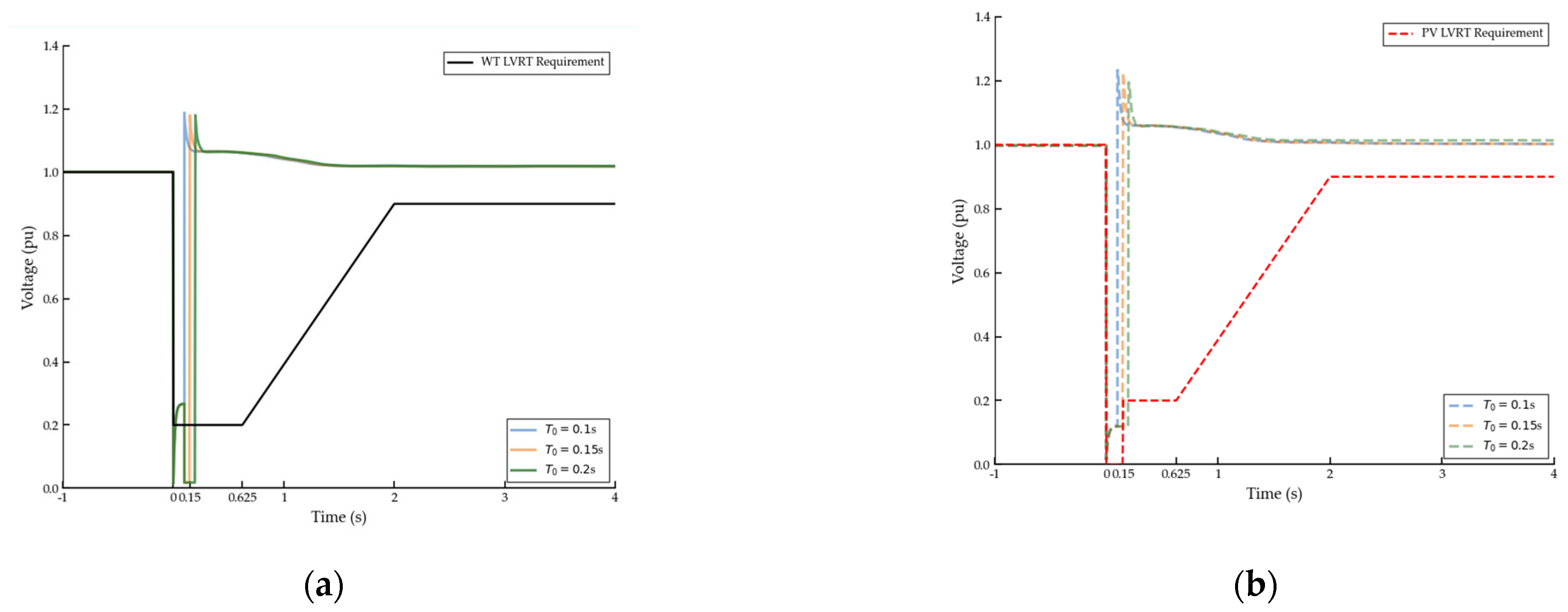
The LVRT requirements for renewable energy in China [29,30] are illustrated in Figure 1. When the voltage of the point of common coupling (PCC) at a wind farm (WF) drops to 20% of its nominal voltage, it must guarantee continuous grid-connected operation for 0.625 s. PV power stations, however, are required to remain continuously connected for 0.15 s even if the PCC voltage drops to zero and subsequently maintain connection when the voltage recovers above 20% of the nominal voltage. Additionally, both WF and PV power plants must remain continuously connected under the condition that the voltage recovers to 90% of the nominal voltage within 2 s after the voltage drop. If the voltage at the renewable energy PCC drops below the voltage ride-through curve, the renewable energy unit is permitted to disconnect from the grid.
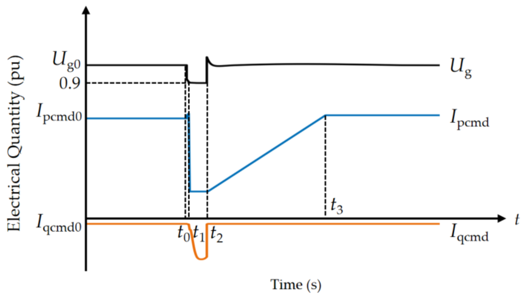
The operational status of a renewable energy generating unit encompasses four states: normal operation state, fault ride-through state, fault ride-through recovery state, and tripped state. During normal operation, the unit employs inner and outer loop control, with the inner loop being the current control loop and the outer loop being the power control loop. Although most renewable energy units enter the LVRT state immediately upon a short-circuit fault due to the voltage dropping below the ride-through threshold of 0.9 pu, in cases where the electrical distance is long, or the fault severity is relatively mild, the PCC voltage may not immediately drop below 0.9 pu. Instead, the voltage may continue to drop throughout the fault duration, eventually leading to LVRT initiation. As shown in Figure 2, t0 is the moment the short-circuit fault occurs, and t1 is the starting moment the renewable energy unit enters the LVRT state. During the time interval t0 to t1, the terminal voltage, although having dropped, remains above 0.9 pu. In this period, the renewable energy unit maintains its normal operation state, simultaneously increasing its active current command to sustain constant output power and increasing its reactive current command to provide a certain level of reactive power support.
At moment t1, the operational status of the renewable energy unit transitions from the normal operation state to the LVRT operation state. At this point, the outer power control loop is bypassed, and the inner current command switches to the LVRT control command. During LVRT, the reactive current command is typically proportional to the depth of the voltage dip. Under the dual constraints of current limitation and reactive power priority, the active current command is usually restricted to a lower level. The control strategy for the reactive current command, Iqcmd, and the active current command, Ipcmd, of the renewable energy unit during LVRT are, respectively, given by the following [31]:
I qcmd = k q 1 ( 0.9 U g ) + I qcmd 0
I pcmd = min ( k p 1 I pcmd 0 , 1 I qcmd 2 )
where kq1 and kp1 are the reactive current coefficient and the active current coefficient, respectively. Ug is the terminal voltage, and Iqcmd0 and Ipcmd0 are the reactive current command value and the active current command value before the renewable energy unit enters the LVRT state, respectively.
When the terminal voltage of the renewable energy unit recovers to above 0.9 pu at moment t2, the unit switches from the LVRT state to the LVRT recovery state. During recovery, the reactive current command immediately returns to the pre-LVRT level, while the active current command recovers at a certain rate:
I qcmd = I qcmd 0
I pcmd = I pcmd 1 + k p 2 ( t t 2 )
When the active current command recovers to its initial pre-LVRT value at moment t3, the LVRT recovery is completed, and the renewable energy unit returns to the normal operation state.

2.1.2. Renewable Energy Tripping

If the renewable energy unit’s LVRT fails, the tripping protection will be triggered. As shown in Figure 3, when the voltage trajectory at the PCC exceeds the LVRT curve, the renewable energy unit will be tripped from the grid after a 0.1 s delay. The moment the PCC voltage exceeds the LVRT capability is designated as t1.
Affected by the differences in LVRT capability requirements shown in Figure 1, the tripping characteristics of wind turbine (WT) units and PV are distinct. For WT, its tripping behavior primarily depends on the depth of the voltage dip rather than the duration of the fault. Tripping protection is triggered when the voltage at the PCC drops below the threshold of 0.2 pu. Conversely, PV exhibits significant sensitivity to the fault duration due to its unique 0.15 s no-tripping limit. If the fault duration T0 is shorter than 0.15 s, the PV can satisfy the LVRT requirements and remain connected. However, if T0 exceeds 0.15 s, tripping will occur if the voltage has not recovered.
In the 0.1 s transient process from moment t1 until tripping, the renewable energy unit is able to utilize its reactive power support capability to boost the PCC voltage. Nevertheless, once the unit trips, the reactive support instantly vanishes, leading to a sharp drop in the PCC voltage until the fault line is cleared and the voltage can recover, as illustrated by the voltage trajectory for T0 = 0.2 s in Figure 3a.

2.1.3. DC Commutation Failure

CF refers to the phenomenon where a thyristor valve, which should cease conduction during the commutation process, fails to recover its blocking capability under reverse voltage in time or when the commutation process is incomplete, causing the valve that should be turned off to re-ignite under forward voltage [32]. The thyristor requires a certain time to recover its forward voltage blocking capability, which corresponds to the minimum extinction angle γmin. The calculation formula for the extinction angle of the DC inverter is given by Equation (5). When the extinction angle is less than γmin, CF will occur. Therefore, it is generally considered that CF occurs when the inverter-side converter bus voltage Uc is less than the critical value Ucmin.
γ = arccos ( 2 I d X c U c + cos β )
Here, Id is the DC current, Xc is the equivalent commutation reactance, and β is the firing advance angle.
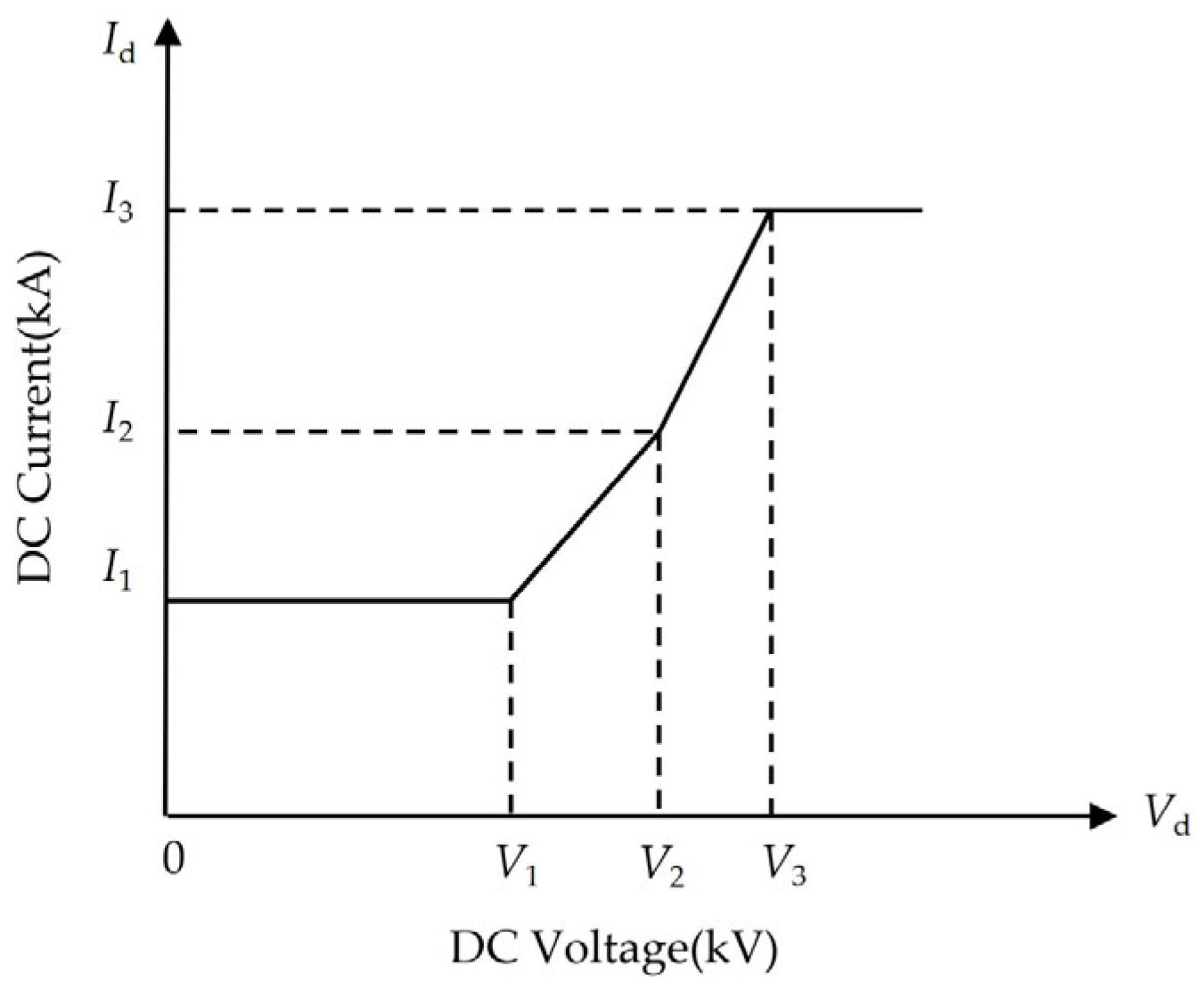
The voltage-dependent current order limit (VDCOL) function [32] can mitigate the occurrence of CF by reducing the DC current when the DC voltage drops, thereby decreasing the commutation angle and increasing the extinction angle. Simultaneously, during the CF recovery process, VDCOL restricts the recovery rate of the DC current, preventing CF recurrence due to excessively fast current recovery. The characteristic curve of the VDCOL function is shown in Figure 4.
In Figure 4, Vd is the DC voltage input to the VDCOL function. The relationship between Vd and Id can be expressed by the function Id = f(Vd), as shown in Equation (6):
I d = f ( V d ) = I 1 V d V 1 I 1 + I 2 I 1 V 2 V 1 ( V d V 1 ) V 1 V d V 2 I 2 + I 3 I 2 V 3 V 2 ( V d V 2 ) V 2 V d V 3 I 3 V d V 3
where I1, I2, and I3 are the DC current parameters of the VDCOL function, and V1, V2, and V3 are the DC voltage parameters of the VDCOL function.
The transient process from a short-circuit fault until the completion of DC commutation failure recovery is illustrated in Figure 5. Uc0, Vd0, and Id0 are the initial values of the inverter-side converter bus voltage, DC voltage, and DC current, respectively. When a short-circuit fault occurs in the receiving-end AC system at moment t0, the inverter-side converter bus voltage drops, and the DC voltage decreases accordingly. Since the DC device operates in constant power mode, the DC current will rise to maintain constant power.
Moment t1 is the instant when the inverter-side converter bus voltage drops below Ucmin, causing DC CF. At this time, both the DC voltage and DC current rapidly drop to zero. After the fault line is cleared, at moment t2, when the inverter-side converter bus voltage is above the threshold Ucmin, the DC enters the CF recovery state. During the recovery process, the DC voltage starts recovering from its minimum setpoint value, and the DC voltage during recovery can be expressed as follows:
V d = V d min + v d ( t t 2 ) t 2 t t 3
where Vdmin is the minimum setpoint value of the DC voltage, and vd is the DC voltage recovery rate. The DC current gradually recovers under the control of the VDCOL function. Moments tv1, tv2, and tv3 shown in Figure 5 correspond to each instant when the DC voltage recovers to V1, V2, and V3, respectively. When the DC current and DC voltage recover to their initial values at moment t3, the DC enters the normal operation state.

2.1.4. Fault Transient Evolution Process

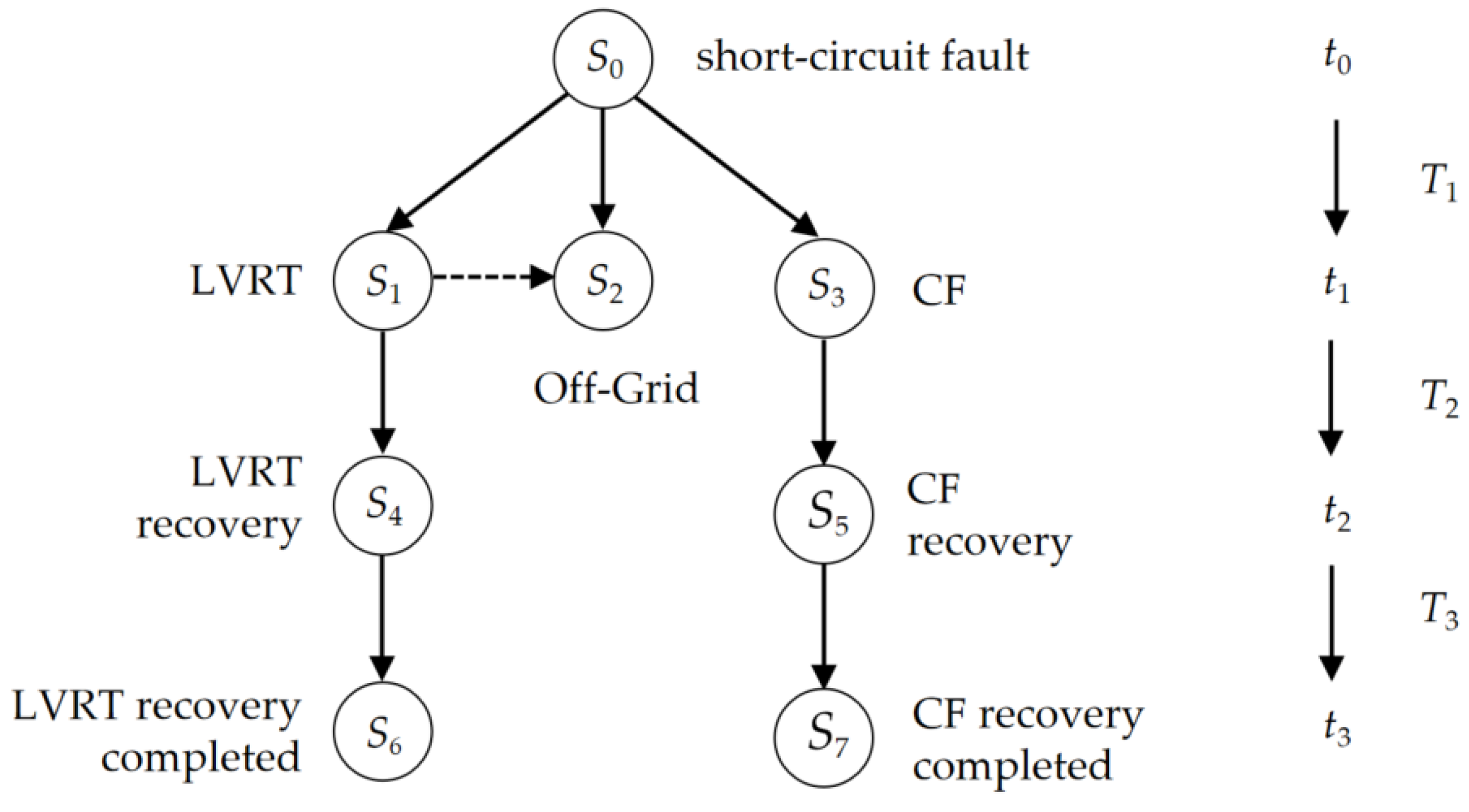
In high-penetration renewable energy power systems, equipment state transitions triggered by short-circuit faults constitute a complex fault transient evolution pattern. To intuitively and quantitatively characterize these evolution patterns and state durations, this paper utilizes a directed weighted graph G (S, E, T) to describe the transient evolution paths associated with renewable energy and DC equipment. Specifically, the fault transient evolution path of any equipment in the system can be represented as a directed path within graph G.
In graph G, S represents the set of different operational states of the system or equipment during the fault period, including the system’s short-circuit fault state, the fault states of renewable energy and DC equipment, the fault recovery state, and the normal operation state. E represents the set of directed transition edges between states, taking a binary value of 0 or 1. Its directionality embodies the logical sequence of fault evolution and physically corresponds to the voltage threshold conditions required for equipment state transitions. T is the weighted adjacency matrix, where the element denotes the state transition time.
The fault transient evolution process is demarcated by four key time instants:
  • t0: The moment the initial short-circuit fault occurs.
  • t1: The starting moment the equipment switches from the normal operation state to the fault operation state, such as the moment the renewable energy unit enters the LVRT state (shown in Figure 2), the instant the renewable energy PCC voltage exceeds the limit (shown in Figure 3), and the moment DC commutation failure occurs (shown in Figure 5).
  • t2: The starting moment the equipment switches from the fault operation state to the fault recovery state.
  • t3: The moment the equipment switches from the fault recovery state back to the normal operation state.
This paper assumes that under normal operating conditions, the system possesses the capability to restore the faulted renewable energy and DC equipment to their normal operation state after the faulty line is cleared. On this basis, the directed weighted graph shown in Figure 6 is constructed to describe the typical transient evolution process of equipment following a short-circuit fault. Here, T1 = t1t0 represents the time required for the equipment to switch from normal operation to fault operation; T2 = t2t1 represents the duration the equipment remains in the fault operation state; and T3 = t3t2 represents the time required for the equipment’s operational parameters to recover to their initial values. In Figure 6, the solid line from "short-circuit fault" to "off-grid" represents the direct off-grid process caused by the short circuit, while the dashed line from "low voltage ride-through (LVRT)" to "off-grid" indicates that equipment typically undergoes an LVRT stage before actual off-grid occurs. This graphical structure aims to illustrate that the root cause of off-grid is the system short-circuit, with LVRT serving as an intermediate transient process that often precedes the final off-grid event.

2.2. Fault Evolution Scenario Generation Based on State Transition and Temporal Features Models

In power systems with a high penetration of renewable energy, the fault transient evolution process is influenced by various factors such as operating conditions, fault characteristics, and equipment control strategies. Its complexity poses a severe challenge to the system’s stable operation. To achieve accurate and fast prediction of the equipment’s operational state S following an initial short-circuit fault, this paper constructs a state transition model and a temporal feature model that map the initial fault to the transient response of renewable energy and DC equipment.
The state transition model is used to determine the existence of the state transition edge E (i.e., whether subsequent faults occur in the equipment), which is treated as a binary classification problem. The temporal feature model is used to quantify the duration T of different states, which is treated as a regression problem. Considering that the transient evolution process of renewable energy and DC equipment involves strong coupling that is difficult to accurately describe using analytical models, this paper establishes models for state transitions and temporal features using data-driven methods based on large-scale simulation data. These extracted features are then used for the generation of fault transient evolution scenarios, laying the foundation for subsequent system risk assessment.

2.2.1. Sample Set Construction

This paper conducts large-scale time-domain simulations based on a receiving-end power grid model with high penetration of renewable energy. By exhaustively setting key parameters such as initial fault location, fault duration, and fault grounding impedance, a massive dataset of fault scenarios and dynamic response data of electrical quantities under different initial faults is obtained. The operation criterion of the protection and control devices of renewable energy and DC devices is defined by the binary table (Ecr.i, Tcr.i), where Ecr.i and Tcr.i are the threshold value and the duration of the event that triggers the protection action of equipment i, respectively. Based on these action criteria, the type and occurrence time of the fault event state transitions can be identified from the electrical quantity data.
(1)
Determination of Output Labels
Based on the assumption in Section 2.1.4 that the power system possesses sufficient reactive power support capability, the state transition model is limited to determining whether the initial short-circuit fault triggers the first level of subsequent faults. For renewable energy tripping events, the PCC voltage drop is severe. According to Equation (1), the voltage is momentarily boosted due to reactive power support, so the moment t1 is deterministic. Specifically, t1 for WT tripping is the instant the fault occurs, while t1 for PV tripping is 0.15 s after the fault occurs; thus, T1 values are 0 and 0.15 s, respectively. For DC commutation failure events, T2 is constrained by the minimum duration (0.2 s) and is generally regarded as a fixed parameter. T3 is determined by the equipment’s control parameters and can be calculated using Equations (4) and (7). Therefore, the temporal feature model in this paper focuses on the time delay T1 from the short-circuit fault to the occurrence of renewable energy LVRT or DC CF and the duration of renewable energy LVRT, T2.
The state transition model uses binary classification labels: the label is set to 1 if renewable energy LVRT, tripping, or DC CF occurs after the initial fault and 0 otherwise. The temporal feature model uses regression labels, and T1 and T2 are extracted from the simulation data.
Furthermore, considering the differences in LVRT requirements between WT and PV, separate state transition models are constructed for WT tripping and PV tripping. Similarly, separate regression models are constructed for the LVRT duration T2 of WT and PV.
(2)
Selection of Input Features
The selection of input features is based on physical mechanism analysis. The fault evolution process is primarily determined by voltage variations, while the degree of voltage dip at each bus is influenced by factors such as the grid operating conditions, initial fault characteristics, and the grid strength surrounding the equipment. Since the state transition model and the temporal feature T1 are related to the severity of the initial fault and the instantaneous response of the grid, while T2 is further affected by the equipment’s internal control strategy and the fault process, the input features are divided into two categories to meet the needs of different prediction tasks.
It is worth noting that although post-fault dynamic features contain direct information regarding the transient evolution process, extracting these features requires a waiting period after fault inception, which would inevitably lead to an assessment delay. To achieve rapid assessment immediately upon fault inception, the input features selected in this paper focus on pre-fault steady-state features and initial fault characteristics. By characterizing the system properties, these features largely dictate the subsequent dynamic trajectory of the system.
When studying the state transition logic and the temporal feature T1, the focus is mainly on the initial fault characteristics and the system operating state before the fault. The input features are shown in Table 1. Given that three-phase short-circuit faults are typically the most severe, this paper assumes all short-circuit faults are three-phase. Consequently, fault grounding impedance and fault duration are selected to quantify the fault severity. Mutual impedance characterizes the strength of the electrical connection between buses; thus, the fault location is represented by the mutual impedance between the equipment and the fault point. Simultaneously, the equivalent impedances at the fault point and the equipment bus are selected to reflect the grid strength at the fault location and the equipment connection point, respectively. Furthermore, the occurrence of a fault depends not only on the magnitude of the voltage dip but also on the initial operating point. Therefore, the pre-fault steady-state voltages at the fault point and the equipment bus are selected as input features.
When studying the temporal feature T2 of renewable energy LVRT, in addition to the features listed in Table 1, it is essential to consider the influence of the equipment’s adjacent area and control coefficients on the LVRT recovery process. The specific supplementary features are shown in Table 2. Generators in the vicinity of renewable energy stations serve as critical reactive power support sources during faults; therefore, the generator bus self-impedance is introduced to characterize their reactive power delivery capability. Simultaneously, the mutual impedance between the equipment and critical adjacent nodes is included to characterize the voltage support strength of the surrounding grid. Additionally, the multiple renewable energy stations short-circuit ratio (MRSCR) is selected to quantify the mutual interaction among multiple stations. Furthermore, the active/reactive current control coefficients during LVRT and the active current recovery coefficient are incorporated to capture the impact of equipment control strategies on the recovery duration.
In Table 2, the calculation formula for MRSCRi is given by the following [33]:
MRSCR i = S a c i P RE i + j i , j i n Z eq i j U i Z eq i i U j P RE j
where i is the renewable energy station number, i = 1, 2,…n; Saci and PREi are the three-phase short-circuit capacity and the injected active power of renewable energy equipment i, respectively; Zeqij is the element at the i-th row and j-th column of the equivalent impedance matrix; and Ui is the PCC voltage of renewable energy equipment i.

2.2.2. Construction of State Transition and Temporal Feature Models

To determine the existence of state transition E via binary classification and quantify the temporal features T1 and T2 via regression, this paper first attempts to use logistic regression and linear regression, respectively, to analyze the linear correlation between the input features and equipment response, aiming to enhance model interpretability. However, considering the widespread strong non-linear coupling characteristics of fault evolution patterns in high-penetration renewable energy power systems, and if the evaluation performance of linear models cannot meet the precision requirements, this paper will select the eXtreme Gradient Boosting (XGBoost) algorithm, which possesses efficient non-linear fitting capability.
(1)
XGBoost Algorithm
XGBoost is an optimized implementation of the gradient boosting decision tree algorithm, known for its efficiency and scalability. It falls under the category of ensemble learning, generating a series of decision trees through a serial iterative method [34]. Compared to deep learning models, which rely heavily on large amounts of sample data, XGBoost is suitable for training medium-to-large-scale structured sample data.
XGBoost accumulates the results of K classification and regression trees (CART) to form the ensemble prediction function:
y ^ i = k = 1 K f k ( x i ) , f k F
where xi is the i-th input sample data, y ^ i is the ensemble prediction value for the i-th sample, and fk(xi) is the prediction value of the k-th decision tree. fk is a function in the function space F, and F represents the set of all possible decision trees.
The objective function of XGBoost consists of two parts: the loss function and the regularization term:
L = i = 1 n l ( y i , y ^ i ) + k = 1 K Ω ( f k )
Ω ( f k ) = γ T + 1 2 λ i = 1 T ω j 2
where l ( y i , y ^ i ) is the loss function, measuring the error between the predicted value and the true value. Ω ( f k ) is the regularization term, used to control model complexity and prevent overfitting. T is the number of leaf nodes; ωj represents the weight of the j-th leaf node; and γ and λ are penalty coefficients.
XGBoost adopts additive training. In the k-th iteration, the objective is to find an optimal new tree, fk, that minimizes the objective function L ( k ) . To solve for the optimal fk, the loss function component is approximated using a second-order Taylor expansion around the current prediction value, yielding the approximated objective function:
L ˜ ( k ) i = 1 n g i f k ( x i ) + 1 2 h i f k 2 ( x i ) + Ω ( f k )
where gi and hi are the first and second derivatives of the loss function, respectively.
(2)
Model Training
The samples are divided into training, validation, and test sets at a ratio of 8:1:1. All input features are standardized to eliminate the influence of different magnitudes. To obtain the optimal model, this paper employs Bayesian optimization combined with five-fold cross-validation for hyperparameter tuning, and the parameter combination with the best average performance is selected as the hyperparameters for the final model.
(3)
Model Evaluation Metrics
For the state transition model, accuracy, precision, recall, and F1-score are adopted to comprehensively evaluate model performance [21]. The specific calculation formulas are as follows:
Acc = TP + TN TP + FP + FN + TN
Pre = TP TP + FP
Re = TP TP + FN
F 1 = 2 Pre × Re Pre + Re
where TP is the number of positive samples correctly predicted as positive; FN is the number of positive samples incorrectly predicted as negative; FP is the number of negative samples incorrectly predicted as positive; and TN is the number of negative samples correctly predicted as negative.
For the temporal feature model, root-mean-squared error (RMSE), mean absolute error (MAE), and the coefficient of determination (R2) are used to evaluate model performance. The specific calculation formulas are as follows:
RSME = 1 n i = 1 N ( y i y ^ i ) 2
MAE = 1 n i = 1 N y i y ^ i
R 2 = 1 i = 1 N ( y i y ^ i ) 2 i = 1 N ( y i y ¯ i ) 2
where n is the number of samples, yi is the actual value of the i-th sample, and y ^ i is the predicted value of the i-th sample.

2.2.3. Fault Evolution Scenario Generation

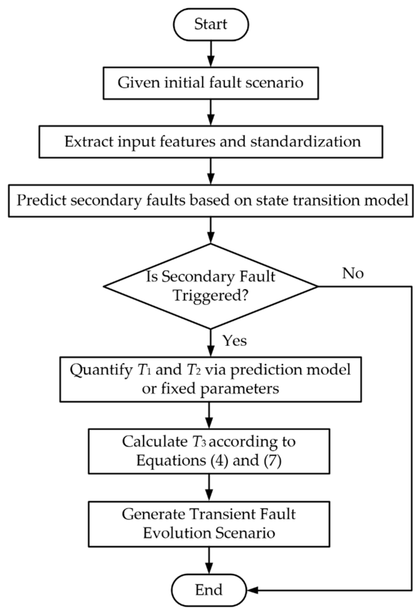
Given the system operating conditions and the initial fault, the complete fault transient evolution scenario triggered by the short-circuit fault in a high-penetration renewable energy power system can be constructed based on the state transition and temporal features models. The specific workflow is shown in Figure 7. The details are as follows:
  • Prepare input feature: For a given initial fault scenario, calculate and extract the relevant electrical quantity features from Table 1 and Table 2. These features are then standardized and used as input for the subsequent models.
  • Predict secondary faults: Input the features into the state transition model. For renewable energy equipment, first predict whether a tripping event occurs. If tripping occurs, the subsequent judgment is terminated. If tripping does not occur, further prediction is made as to whether LVRT occurs. For DC equipment, the prediction of whether CF occurs is performed in parallel.
  • Quantify temporal feature parameters: For WT and PV predicted to trip, T1 is set to 0 and 0.15 s, respectively. For renewable energy units judged to undergo LVRT, T1 and T2 are predicted based on the temporal feature model. For DC equipment, where CF is predicted, T1 is predicted, and T2 is set to the fault duration value of 0.2 s. T3 is calculated according to Equations (4) and (7) by using the equipment’s control parameters in all cases.
  • Generate fault transient evolution scenario: Integrate the initial fault information, the sequence of subsequent fault states for each equipment, and the temporal feature parameters. Then, obtain the fault evolution path for each renewable energy unit and DC device, ultimately generating the complete fault evolution scenario.

2.3. Risk Assessment of the Fault Transient Evolution Process

An initial short-circuit fault in the AC system may trigger large-scale renewable energy units to undergo LVRT or even tripping and simultaneously lead to CF in multiple converter stations. This results in a severe active power deficit, which can consequently induce rotor angle stability and frequency stability problems. This paper defines the fault transient evolution risk as the equivalent active power loss R to quantify the impact of the active power deficit from renewable energy and DC equipment during the transient process on system security and stability.
During the fault transient evolution process, the power deficit is inherently a time-varying instantaneous active power deviation, and its comprehensive impact can be characterized by the time integral of this deviation, representing an energy deficit W. However, risks caused by events such as renewable energy tripping or DC blocking typically manifest as sustained power deficits. To facilitate the comprehensive assessment of both transient energy risks and sustained power risks under a unified dimension, this paper introduces an electrical quantity conversion coefficient, λE, to convert the transient energy deficit W into an equivalent active power loss R over a specific time scale Teq:
R = W / T eq = λ E W
Referring to the typical time scale of transient stability analysis [35], Teq is selected as 10 s in this paper. Consequently, λE is determined to be 0.1 s−1, implying that a transient energy deficit of 10 MW·s is equivalent to an active power loss of 1 MW.
Since precise active power during the transient process is difficult to obtain directly through analytical methods, the risk of each fault event is quantitatively assessed using a phased simplified calculation approach.

2.3.1. Renewable Energy LVRT Risk

The renewable energy LVRT risk Rlvrt is expressed as the equivalent power value obtained by converting the time integral of the active power deficit during the fault transient process via λE:
R lvrt = λ E t 0 t 3 Δ P lvrt d t
where λE is the electrical quantity conversion coefficient, used to convert the electrical energy risk to power risk, with a value of 0.36 kW/Wh, meaning a power deficit of 10 kW·s is equivalent to 1 kW of renewable energy tripping; ΔPlvrt is the active power deficit of the renewable energy station during the fault transient process, defined as the difference between the pre-fault steady-state power Plvrt0 and the instantaneous power Plvrt:
Δ P lvrt = P lvrt 0 P lvrt
The instantaneous power can be calculated from the components of the terminal voltage and current in the synchronous rotating reference frame:
P lvrt = U d I d + U q I q
where Ud and Uq are the d-axis and q-axis components of the terminal voltage, respectively; Id and Iq are the d-axis (active) current and q-axis (reactive) current. Since the synchronous rotating reference frame is usually synchronized with the angle of the phase-locked loop (PLL), and assuming the PLL remains stable during the transient process, the Uq value is approximately zero; thus, PlvrtUdId.
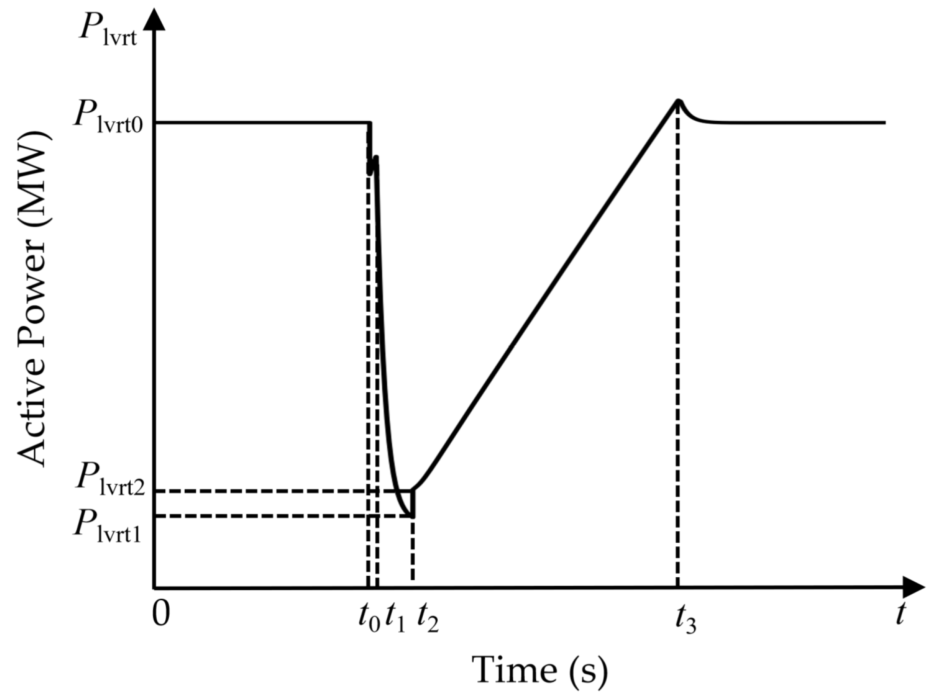
As is known from Section 2.1.1, the process from the occurrence of a short-circuit fault to the completion of LVRT recovery involves three stages. The LVRT risk of the renewable energy unit is the sum of the risk values for these three stages. Figure 8 shows the change curve of renewable energy terminal active power over time, and the active power loss for each stage is as follows:
  • Stage 1 (t0 to t1): Under severe transient disturbance, the voltage of most renewable energy units drops below the LVRT threshold of 0.9 pu. immediately upon fault occurrence, meaning T1 tends to be zero. Additionally, some renewable energy units may initiate LVRT due to voltage drop during the fault duration, where T1 is relatively short. Furthermore, under the effect of electrical control, the reduction in active power is minor, so the risk value for this stage is approximated as zero:
R lvrt 1 = λ E t 0 t 1 ( P lvrt 0 P lvrt ( t ) ) d t 0
2.
Stage 2 (t1 to tcl): In this stage, the active current is restricted to a lower level, and the active power rapidly decreases to a minimum value, Plvrt1. The recovery initiation moment t2 depends on the depth of the voltage drop: if the drop is deep, t2 equals the fault clearance moment tcl; if the drop is mild, the station may recover in advance using its own reactive power support capability, so t2 < tcl. Theoretically, t2 is the end moment of LVRT, but in the case where t2 < tcl, the voltage maintains at approximately 0.9 pu during the period t2 to tcl; thus, the power is considered to remain stable at Plvrt1. Therefore, to simplify the calculation, the upper limit of integration is taken as tcl, and the equivalent power loss for this stage is as follows:
R lvrt 2 = α λ E t 1 t cl ( P lvrt 0 P lvrt ( t ) ) d t = α λ E ( P lvrt 0 P lvrt 1 ) ( T 0 T 1 )
where α is a coefficient, when t2 = tcl, α is 1; when t2 < tcl, α is 0.5, indicating a slow decrease in active power to Plvrt1. The value of Plvrt1 depends on whether T1 = 0: when T1 = 0, Plvrt1 ≈ 0; when T1 ≠ 0, Plvrt1 ≈ 0.9 kp1Plvrt0.
3.
Stage 3 (tcl to t3): In this stage, the renewable energy unit enters the recovery state. After the fault is cleared, the voltage maintains at approximately 1.0 pu, and the active current gradually recovers from the endpoint of the LVRT process at a certain slope. Therefore, the equivalent power loss for this stage is as follows:
R lvrt 3 = λ E t cl t 3 ( P lvrt 0 P lvrt ( t ) ) d t = λ E ( P lvrt 0 P lvrt 2 ) T 3 / 2
where Plvrt2 is the active power at the instant of fault clearance, with a value of kp1Plvrt0; and T 3 = t3tcl.

2.3.2. Renewable Energy Tripping Risk

The renewable energy tripping risk Roff includes the transient power loss before tripping Roff1 and the sustained power deficit caused by the tripping:
R off = λ E t 0 t off Δ P off d t + P off 0
where toff is the instant the unit trips, considering a 0.1 s protection delay, toff = t1 + 0.1 s; ΔPoff is the change in active power of the renewable energy station during the transient process before tripping; and Poff0 is the pre-fault steady-state active power value of the renewable energy station.
For WT, t1 = t0. As shown in Figure 9a, during the transient process before tripping, the voltage drops severely, and the presence of the low-voltage current limiting function for active current means the active current is zero; thus, the active power is also zero.
Therefore, the total equivalent active power loss for the WT tripping is as follows:
R off , wt = 0.1 λ E P wt 0 + P wt 0
where Pwt0 is the pre-fault steady-state active power value of the WT.
For PV units, t1 = t0 + 0.15. As shown in Figure 9b, during the transient process from t0 to toff, the active power is also zero due to the severe voltage drop. At the moment of fault clearance, the recovery of voltage and active current causes a sudden increase in active power, which then returns to zero at the tripping moment. Since the power deficit is the primary concern and this part of the transient process is very short, the power loss during this period is ignored. Therefore, the equivalent power loss for PV tripping is as follows:
R off , pv = λ E P pv 0 T 0 + P pv 0
where Ppv0 is the power value of the PV unit under pre-fault steady-state conditions.

2.3.3. DC Commutation Failure Risk

The DC commutation failure risk Rcf is as follows:
R cf = λ E t 0 t 3 Δ P cf d t
where the DC power deficit ΔPcf is the difference between the pre-fault steady-state power Pcf0 and the instantaneous power Pcf:
Δ P cf = P cf 0 P cf
where Pcf can be calculated using the DC voltage Vd and DC current Id, i.e., Pcf = VdId.
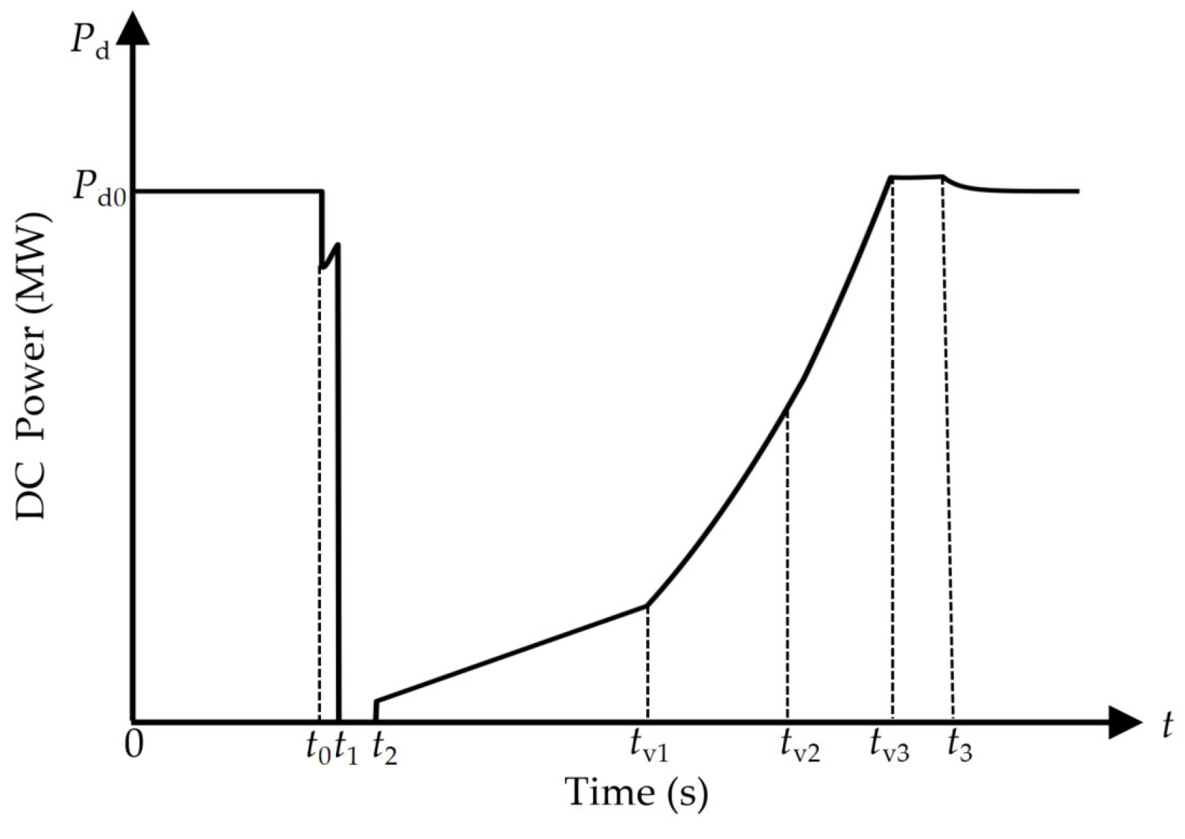
The process from the occurrence of a short-circuit fault to the completion of DC CF recovery also involves three stages. The DC CF risk is the sum of the risk values for these three stages. The change curve of DC power over time is shown in Figure 10. The active power loss for each stage is as follows:
  • Stage 1 (t0 to t1): The duration of the transient process T1 in this stage is short, and under the control of the DC, the reduction in active power is minor. Therefore, the risk value for this stage is assumed to be zero:
R cf 1 = λ E t 0 t 1 Δ P cf ( t ) d t 0
2.
Stage 2 (t1 to t2): During the commutation failure, the active power rapidly drops and remains at zero. The risk for this stage is as follows:
R cf 2 = λ E t 1 t 2 Δ P cf ( t ) d t = λ E t 1 t 2 P cf 0 d t = λ E P cf 0 T 2
3.
Stage 3 (t2 to t3): In this stage, the DC enters the recovery state. During the t2 to tv3 phase, the active power gradually recovers from zero. This recovery can be calculated using the analytical expressions in Equations (6) and (7), based on the VDCOL curve and the recovery control strategy. In the tv3 to t3 phase, the DC power basically recovers to its initial steady-state value, and the system operates in constant power mode, so the power loss is approximated as zero. Therefore, the equivalent power loss for this stage is as follows:
R cf 3 = λ E t 2 t 3 Δ P cf ( t ) d t λ E t 2 t v 3 P cf 0 - P cf ( t ) d t

3. Results

3.1. Simulation Case

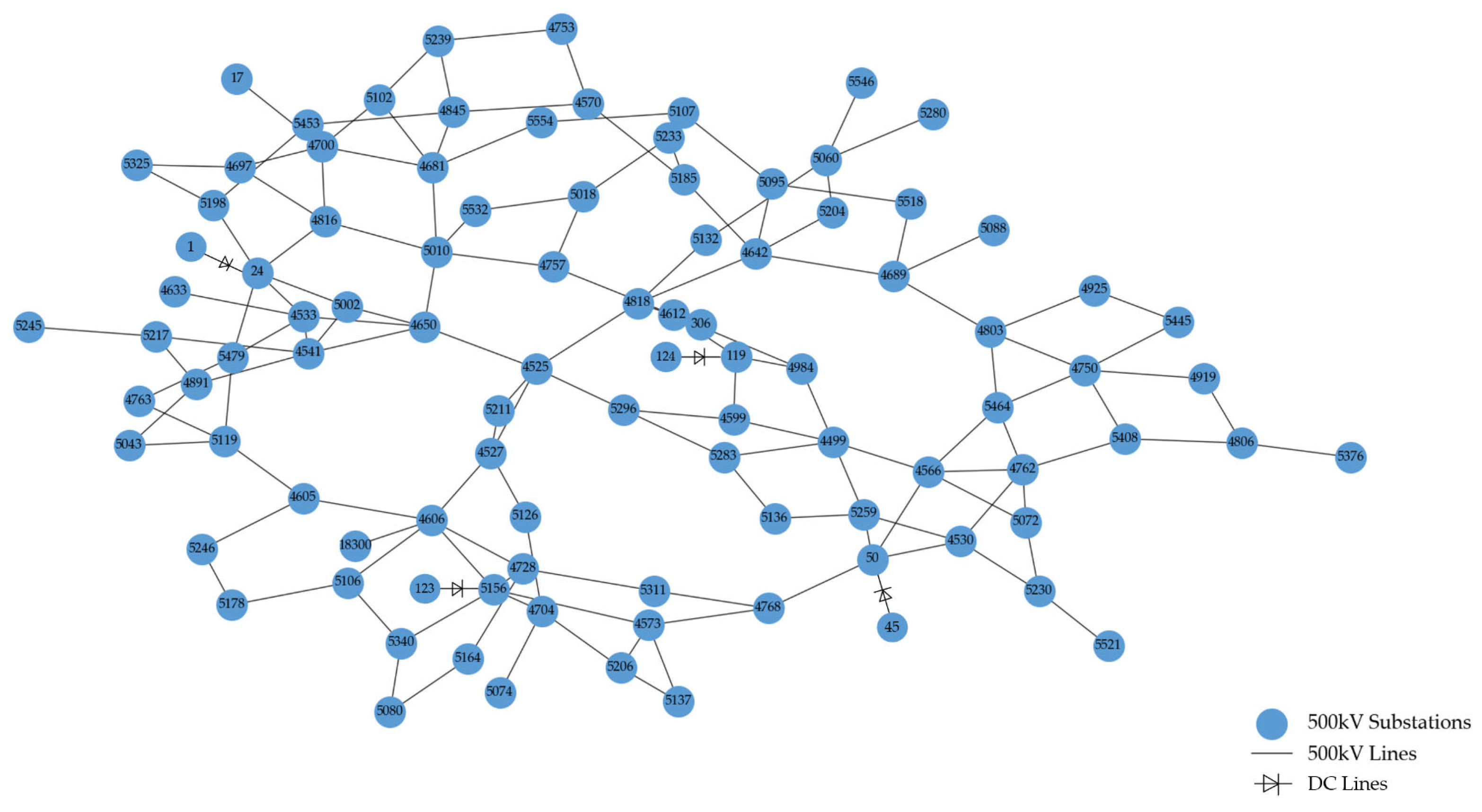
This paper uses a provincial power grid located within the North China and Central China Power Grid for analysis to verify the effectiveness of the proposed method. Figure 11 shows the structural diagram of the 500 kV AC lines and DC lines in the provincial power grid. The total load in this regional grid is 80.33 GW. Regarding the power source composition, it includes four DC links receiving 17.37 GW; 198 thermal power units generating 39.36 GW; 85 WF generating 7.81 GW; and 170 PV generating 18.88 GW. The proportion of renewable energy generation reaches approximately 40%. The system comprises 201 sections of 500 kV AC lines and 1740 sections of 220 kV AC lines. The simulations are conducted using the STEPS platform [36], and the simulation time step is 5 ms. The adopted renewable energy models are electromechanical transient models, with control strategies implemented in accordance with the control logic described in Section 2.1.1 and Section 2.1.2. For the convenience of analysis, the case studies in this paper assume that the initial short-circuit fault always occurs at 1 s. All tests are performed on a personal computer with an Intel 2.10 GHz CPU and 16 GBRAM.

3.2. Performance Assessment of State Transition and Temporal Feature Models

This paper constructed the dataset using large-scale time-domain simulations. The fault locations cover the 500 kV and 220 kV transmission lines in the system; the fault duration selects five time values ranging from 0.1 s to 0.2 s; and the fault grounding impedance selects eight values between 0 and 0.01 pu, covering different degrees of fault severity from metallic short circuits to faults grounded through small resistors. By exhaustively traversing the above parameter combinations, a total of 2960 fault scenarios were ultimately generated.
Considering that a single fault scenario involves the response of multiple renewable energy stations and DC equipment, different numbers of sample sets were constructed for different tasks. The sample size for the LVRT state transition model is 51,688; the sample size for the LVRT temporal feature T1 model is 22,871; and the sample sizes for the LVRT temporal feature T2 model for WF and PV stations are 6858 and 16,013, respectively. The sample sizes for the tripping event state transition model for WFs and PVs are 2724 and 1824, respectively. The sample sizes for the CF state transition model and temporal feature model are 2598 and 1186, respectively.
The state transition model and the temporal feature T1 model both utilize the 10-dimensional input features listed in Table 1. Specifically, all impedance features are decomposed into their resistive (real) and reactive (imaginary) components to serve as independent input features. The LVRT temporal feature T2 model expands this to a total of 34 dimensions by incorporating the supplementary features from Table 2. The added 24-dimensional features include the self-impedances of the top-five electrically closest critical generators and the mutual impedances of the top-five adjacent buses (similarly decomposed into resistance and reactance, contributing 20 dimensions), in addition to the MRSCR and three LVRT control coefficients. Given that electrical coupling strength decays with increasing electrical distance, selecting the nearest five generators and buses effectively covers the voltage support area, while avoiding the feature redundancy and model overfitting caused by introducing excessive weakly coupled distal buses.
In terms of model training and parameter optimization, corresponding strategies were adopted for different models: grid search was used for logistic regression and linear regression models to determine the optimal combinations. For the XGBoost model, which possesses a more complex parameter space, Bayesian optimization was employed for hyperparameter tuning.

3.2.1. Performance Metrics of State Transition and Temporal Feature Models

The performance of the various state transition models and temporal feature models on the test set is shown in Table 3 and Table 4.
As indicated in Table 3, the logistic regression model performs poorly because the threshold for identifying LVRT in renewable energy is relatively high (0.9 pu.), and the depth of voltage dip at the grid connection point is highly coupled with non-linear factors such as control strategies, reactive power support capability, and grid strength. Although non-linear models like SVM and neural networks improved performance to some extent, SVM suffers from long training times when processing large-scale samples. In contrast, the XGBoost model not only achieved the best results across all performance metrics but also maintained high training efficiency. This demonstrates XGBoost’s superiority in handling such strongly coupled non-linear problems; therefore, it has been selected as the state transition discrimination model for LVRT.
On the other hand, renewable energy tripping events and DC CF typically occur in scenarios with more severe fault levels, making them relatively easier to identify. For these tasks, the simple logistic regression model already performs excellently, with recall rates exceeding 99%, effectively preventing missed detections. Given its negligible training time, logistic regression was directly selected as the final model for these two categories of tasks.
Table 4 presents the performance comparison of the temporal feature models. Due to the high non-linearity of the temporal parameters in fault evolution, the linear regression model exhibits significant errors. Among the non-linear models, neural networks and SVM also show poor fitting results and require longer training times. In contrast, the XGBoost model demonstrates superior training efficiency and prediction accuracy. The R2 values for the temporal feature models across different fault events are consistently high, and the RMSE is kept within two simulation time steps (10 ms). This allows for a relatively precise capture of the duration of different states during the fault evolution process, establishing a foundation for the subsequent approximate calculation of power loss risks. The optimal hyperparameter combinations for the final selected XGBoost model are detailed in Table A1.

3.2.2. Model Interpretation Based on SHAP

For the state transition models of renewable energy tripping and DC CF, the linear structure of logistic regression allows for the direct quantification of feature contributions through weight coefficients. The coefficient analysis results indicate that mutual impedance consistently occupies a dominant position in the feature importance ranking, confirming that the electrical distance between the equipment and the fault point is the critical factor determining fault occurrence. Furthermore, the weight coefficients for the self-impedance of the short-circuit point and the fault grounding impedance are also significant. This physically reflects the direct driving effect of grid strength at the fault location and the fault severity on triggering such events.
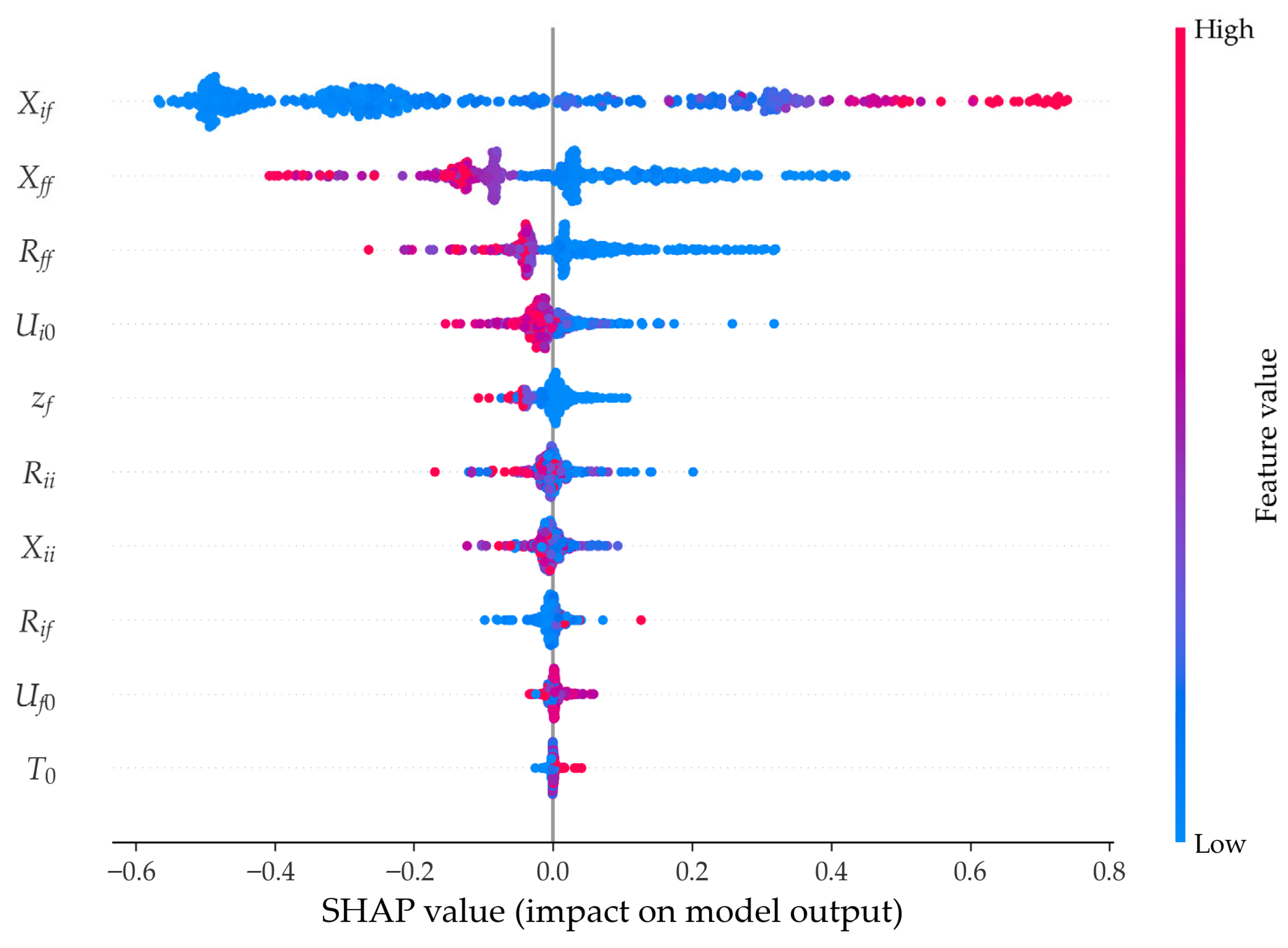
To enhance the interpretability of the XGBoost model, this paper introduces Shapley additive explanations (SHAP) for visual analysis. Figure 12 illustrates the SHAP values for the renewable energy LVRT state transition model, with features ranked by importance from top to bottom. The results indicate that mutual impedance Xif ranks highest, serving as a proxy for the electrical distance between the short-circuit point and the equipment; this identifies it as the most critical factor determining the occurrence of LVRT. Specifically, the high-value samples (red dots) of Xif are concentrated in the positive SHAP value region, revealing that a closer electrical proximity results in more severe fault impact on the renewable energy units, thereby increasing the probability of triggering an LVRT event.
Furthermore, the equivalent impedance of the short-circuit point (Xff, Rff) follows in importance, reflecting the grid strength at the fault location. Its low-value samples (blue dots) correspond to positive SHAP values, indicating that a smaller equivalent impedance at the fault point leads to higher short-circuit currents and more significant voltage dips, which more easily trigger the LVRT response.
Since the initial voltage at the fault point typically remains at 1.0 pu before the fault, it has little influence on the occurrence of the fault event. Additionally, because the severe voltage drop mainly occurs at the instant of the fault, its correlation with fault duration is weak.
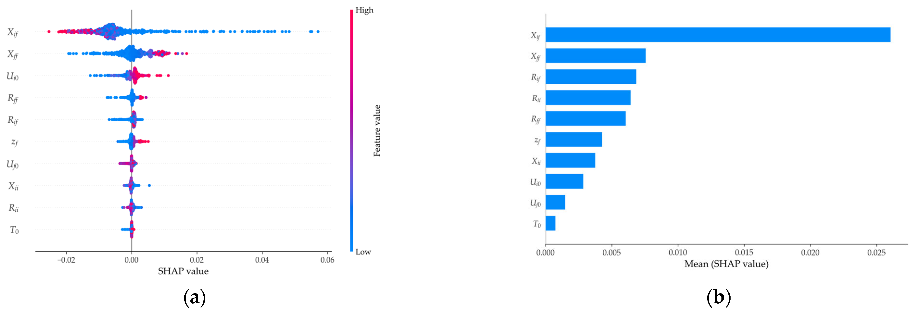
Figure 13 compares the differences in feature importance for the temporal feature T1 between renewable energy LVRT and DC CF. The results show that mutual impedance remains dominant, indicating that the fault response delay T1 fundamentally depends on the depth and speed of the voltage drop at the instant of the fault. For renewable energy LVRT, the weight of the equipment’s initial voltage Ui0 is high. This is because the LVRT action threshold (0.9 pu) is high, and minor fluctuations in Ui0 significantly affect the time required for the voltage to drop below the threshold. For DC commutation failure, mutual impedance is still the dominant factor, but the weight of self-impedance increases significantly. This is because DC commutation failure is not only affected by the AC fault-induced voltage drop but is also closely related to the short-circuit capacity of the converter bus and the strength of the receiving-end power grid.
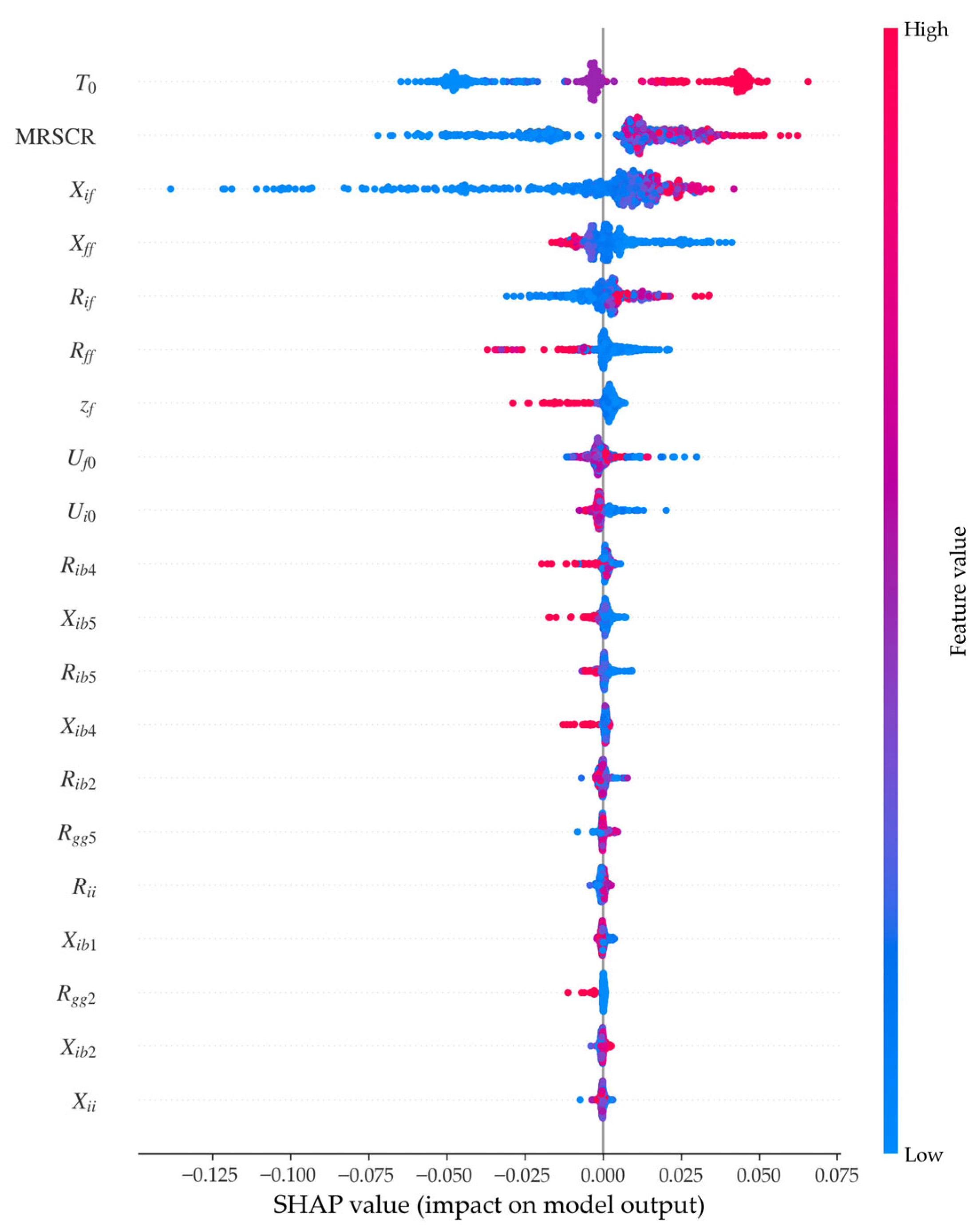
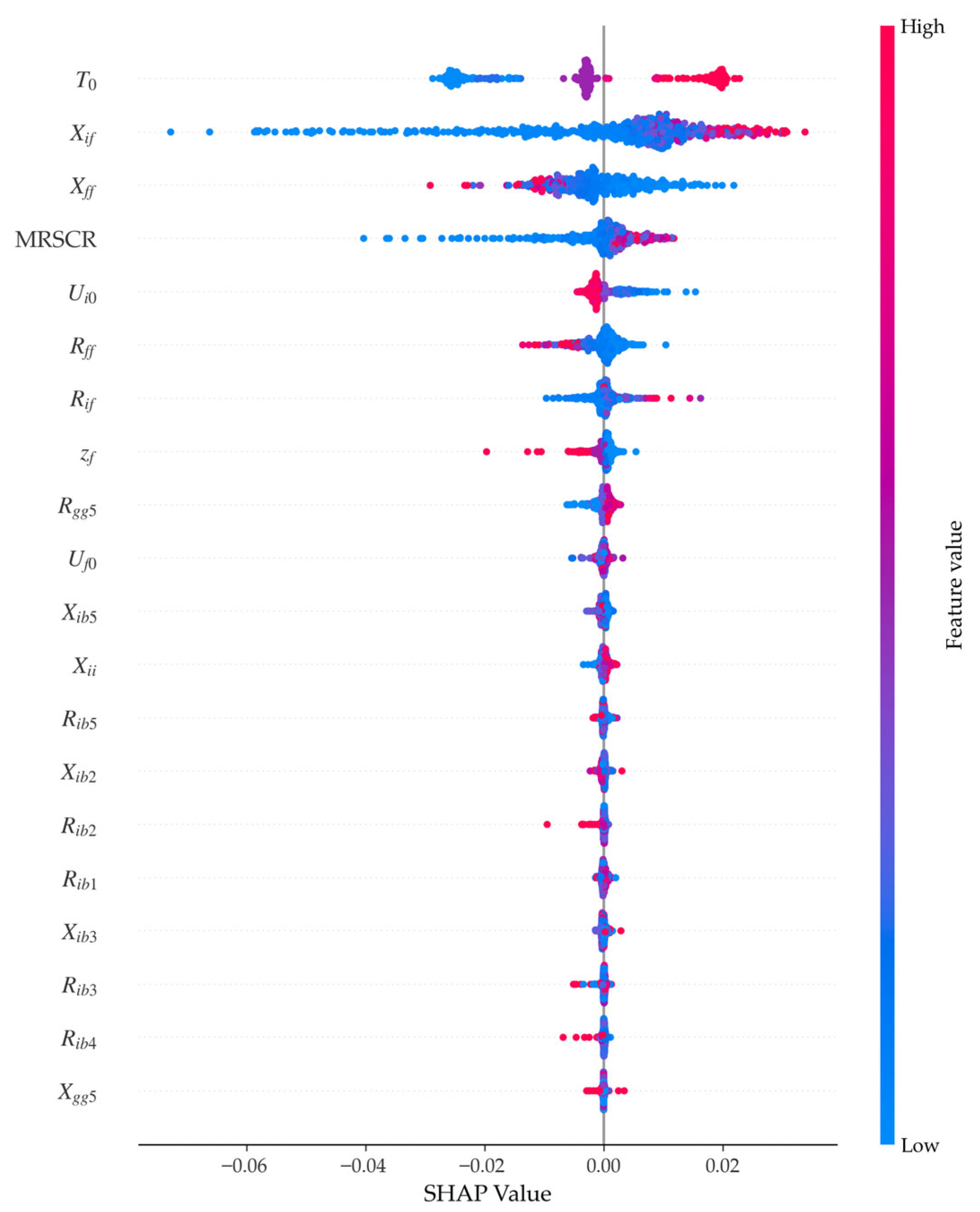
Figure 14 and Figure 15 present the SHAP values of the top 20 key features in the LVRT duration T2 for WFs and PVs. Analysis indicates that the length is not only influenced by the dominant factors of the fault-triggering stage (mutual impedance and short-circuit point equivalent impedance) but is also significantly constrained by the MRSCR and the fault duration. MRSCR reflects the grid strength in the renewable energy connection area. When MRSCR is low, system support capability is insufficient, and voltage recovery is slow, leading to a longer T2 duration. Since most renewable energy units experience a deep voltage drop, their LVRT recovery can only follow the fault clearance moment. Thus, the importance of fault duration is also high.
The mutual impedance between the renewable energy unit and surrounding buses directly characterizes the strength of the electrical connection between the nodes. Similarly, due to the clustered distribution of renewable energy, near-area buses are similar, and the mutual impedance of slightly more distant buses can effectively capture differences in PCC voltage recovery, thus having a higher weight.
The self-impedance of thermal power units characterizes their reactive power delivery capability. Thermal units located near renewable energy clusters serve as critical reactive power support sources for maintaining voltage during a fault. However, due to the concentrated distribution of renewable energy stations, the nearest thermal units are often identical across different samples, resulting in low feature distinctiveness. For the T2 of PVs, the self-impedance importance of the fifth nearest thermal unit, which is at a greater electrical distance, is actually higher. This suggests that T2 is influenced by subtle differences in system support sources over a broader geographical range.
Furthermore, Figure 14 and Figure 15 indicate that T2 has a weak correlation with the renewable energy unit’s own control parameters. This suggests that under severe faults, the external system response far outweighs the limited reactive power support capability of the station itself.

3.2.3. Results of Risk Assessment for the Transient Evolution Process

To verify the accuracy of the phased approximate calculation method for the fault transient evolution process risk assessment, this paper sets up different initial short-circuit faults. Then, the key temporal feature parameters are extracted based on time-domain simulation results to perform the approximate risk assessment calculation, and these results are compared with the actual risk value Rsim obtained from the simulation results.
Table 5 and Table 6 show the key parameters and risk value calculation results during the renewable energy LVRT process. The comparison results show that the relative error is controlled within 5% for all cases except PV 21085, whose relative error is slightly higher, reaching 7.14%. It should be noted that this is mainly because the risk value of this case is relatively small (2.395 MW), which causes a minor absolute error to magnify the percentage value of the relative error, while the absolute error (0.171 MW) remains within an acceptable range.
Table 7 shows the risk assessment results during the transient process of WFs and PVs tripping. Although the 0.1 s protection delay process before tripping introduced a minor error, the overall accuracy of the approximate calculation remains excellent.
Table 8 shows the risk assessment results during the transient process of DC CF. Analysis indicates that although the method ignores minor power fluctuations during the T1 period for calculation simplification, the assessment validity is ensured by the close fitting of the power recovery process based on the VDCOL curve.
From the comparative results of the transient evolution process risk assessment for different fault events, it is clear that the approximate calculation method proposed in this paper can accurately evaluate power loss.

3.2.4. Fast Risk Assessment Results Based on Fault Evolution Path

After setting the initial fault, the equipment status and temporal parameters are first predicted based on the state transition model and temporal feature model to obtain the fault evolution path. Then, the transient process risk value is calculated based on this evolution path. Finally, the predicted results are compared with the actual evolution process and risk values obtained from time-domain simulation to verify the effectiveness of the proposed method.
(1)
Initial fault 1: the fault line is a 500 kV line (5132, 4818), the fault duration is 0.11 s, and the fault grounding impedance is 0.005 pu.
Under initial short-circuit fault 1, the state transition model and temporal feature model predict that 17 WFs and 40 PVs will undergo LVRT, and the calculated total power loss is 272.143 MW. Time-domain simulation results show that the actual LVRT occurred in 16 WFs and 40 PVs, with a total power loss of 275.135 MW. The comparative analysis of the renewable energy LVRT caused by initial fault 1, across multiple dimensions including fault identification results, key temporal parameter prediction accuracy, and total power loss assessment, is presented in Table 9. The detailed comparison results between the predicted fault evolution path and time-domain simulation for initial fault 1 are shown in Table A2.
From the comparison results in Table 9, it can be seen that the machine learning models exhibit excellent performance in predicting the fault evolution path for the initial fault. Although the model accuracy is 98.25%, with a minor misjudgment on WF LVRT, the recall rate reaches 100%, successfully identifying all renewable energy stations undergoing LVRT. In temporal feature prediction, the T1 prediction error is less than one step size. And with a high prediction error for T2, the total equivalent power loss error compared to the actual value is only 1.08%.
Under initial short-circuit fault 1, it is predicted that the DC link (124, 119) will experience CF at the instant of the fault. The equivalent power loss obtained through approximate risk assessment is 254.162 MW, while the equivalent power loss obtained from time-domain simulation is 251.032 MW, with an error of only 1.24%.
(2)
Initial fault 2: the fault line is a 220 kV line (5418, 18,330), the fault duration is 0.14 s, and the fault grounding impedance is 5.6 × 10⁻⁵ pu.
Under initial short-circuit fault 2, the state transition model predicts that two WFs will undergo tripping, and two WFs and two PVs will undergo LVRT. Since the renewable energy units around this fault location are relatively dispersed and far from the DC link, the model prediction results are exactly the same as the time-domain simulation results. The detailed comparison of the evolution path is shown in Table 10. As demonstrated in Table 10, the proposed graph-based fault transient evolution model successfully reconstructs the complete state transition process of the renewable energy units. The high consistency between the predicted path and the simulation results serves as a direct verification of the effectiveness of the graph modeling approach, confirming that the constructed directed weighted graph G effectively captures the state transition logic and temporal characteristics of the transient process.
The comparison results between the approximate risk value calculation for each renewable energy station and the actual risk value obtained from time-domain simulation are detailed in Table 11.
From Table 11, it can be seen that under initial fault 2, the relative errors for WF 21238 and WF 21239 reach 8.22% and 7.63%, respectively. Consistent with the analysis in Table 6, these magnified percentages are attributed to the small absolute risk values (2.4 MW and 5.9 MW). The absolute prediction errors (0.2 MW and 0.45 MW) are negligible compared to the dominant tripping loss (141.47 MW). Crucially, the total equivalent power loss obtained through approximate calculation is 160.088 MW, and the actual total equivalent power loss calculated by time-domain simulation is 160.562 MW, with an absolute error of only 0.474 MW. This fully demonstrates that the proposed method has high reliability for the rapid assessment of overall system risk.
For initial faults 1 and 2, the fault evolution paths generated by the state transition model and the temporal feature model are extremely fast, taking only 0.023 s and 0.024 s, respectively. In contrast, the time-domain simulations take 14.643 s and 25.815 s. These results demonstrate that the proposed method offers a significant improvement in efficiency, enabling the rapid identification of subsequent fault events and evolution risks following an initial fault.
In summary, the proposed state transition model and temporal feature model can predict the fault evolution path with satisfactory performance, and the proposed phased approximate calculation method can also achieve quantitative calculation of the equivalent active power loss during the transient process, thereby providing effective support for system operation and decision making.

4. Conclusions

This paper proposes a rapid risk assessment method based on the fault transient evolution process to address issues such as the complexity of transient evolution and the difficulty of risk quantification in high-penetration renewable energy receiving-end grids under short-circuit faults. By integrating physical mechanism analysis with a data-driven approach, the method achieves reliable prediction of fault evolution paths and rapid quantification of transient active power deficit. The main conclusions drawn are as follows:
  • Validation using a provincial grid case study demonstrates that the proposed fault transient evolution path prediction method, based on state transition and temporal feature models, not only effectively identifies critical events like renewable energy LVRT but also quantifies key temporal parameters, thereby yielding the complete transient evolution scenario following the fault.
  • The proposed phased simplified calculation of the equivalent power loss method can rapidly and effectively quantify the risk associated with complex transient evolution processes, holding significant importance for supporting quick decision making and developing emergency control strategies.
  • Feature importance analysis indicates that the triggering of subsequent faults is primarily influenced by mutual impedance. The duration of LVRT is no longer solely determined by fault severity but is largely affected by system strength, fault duration, and the supporting capability of critical nodes.
This paper focuses on the typical transient evolution process under conventional operating conditions. It is worth noting that in scenarios with insufficient reactive power support, the post-fault voltage may exhibit sluggish recovery or repetitive dips. These phenomena can subsequently induce complex cascading failures, such as the successive LVRT and tripping of renewable energy units, as well as successive commutation failures in DC systems. The evolution mechanisms and risk assessment of such cascading events present significantly greater challenges. Therefore, future research will be dedicated to investigating the transient evolution of cascading failures driven by insufficient reactive power support.

Author Contributions

Conceptualization, S.Q., C.L., H.T. and C.M.; methodology, S.Q., Y.P. and C.L.; software, S.Q. and Y.P.; validation, S.Q.; formal analysis, Y.P.; investigation, S.Q.; resources, C.L., H.T. and C.M.; data curation, Y.P. and H.T.; writing—original draft preparation, S.Q.; writing—review and editing, Y.P., C.L., H.T. and C.M.; visualization, S.Q.; supervision, C.L., H.T. and C.M.; project administration, H.T. and C.M.; funding acquisition, H.T. and C.M. All authors have read and agreed to the published version of the manuscript.

Funding

This work was supported by the Science and Technology Project of the State Grid Corporation of China [Project Title: “Research on Uncertainty Analysis and Evaluation and Coordinated Prevention and Control Technology of Cascading Failures in New Power System (5100-202316431A-3-2-ZN)”].

Data Availability Statement

The original contributions presented in this study are included in the article. Further inquiries can be directed to the corresponding author.

Conflicts of Interest

The authors Hao Tian and Changhui Ma are employed by the State Grid Shandong Electric Power Research Institute. The remaining authors declare that this research was conducted in the absence of any commercial or financial relationships that could be construed as potential conflicts of interest.

Appendix A

Table A1. Optimal hyperparameter combination for the XGBoost model.
ModelMax
Depth
Learning Rateα *λ *Subsample *Colsample *
_Bytree
State transition model-LVRT *60.1020.9760.7790.9150.763
Temporal feature model-LVRT T150.1000.80.9
Temporal feature model-WF LVRT T240.17101.01.01.0
Temporal feature model-PV LVRT T260.101.00.8480.7
Temporal feature model-CF T130.10.0500.70.7
* α and λ are the L1 regularization weight and L2 regularization weight, respectively; subsample represents the fraction of samples randomly sampled for each tree; and colsample_bytree represents the fraction of features randomly selected when building each tree.
Table A2. Comparison of fault evolution path prediction and simulation results under initial fault 1.
Renewable Energy StationPlvrt0
(MW)
Prediction
T1 (s)
Simulation
T1 (s)
Prediction T2 (s)Simulation
T2 (s)
T3 (s)Rlvrt
(MW)
Rlvrt,sim
(MW)
WF 1831587.5000.0850.111.0553.1853.211
WF 1831687.5000.090.111.5856.6437.024
WF 1832187.5000.090.110.7052.2792.287
WF 1832287.5000.090.110.993.4523.547
WF 2113184000.110.111.064.9314.732
WF 2115484000.090.111.244.0494.192
WF 2120684000.0750.110.7052.1500.003
WF 2120887.5000.080.111.395.2415.472
WF 2120987.5000.0750.111.053.1463.062
WF 2121087.5000.080.111.224.1264.255
WF 2121187.5000.0750.110.7052.2402.199
WF 21240105000.110.110.8254.1873.725
WF 2124187.5000.0850.111.4155.3465.522
WF 2124287.5000.080.111.0553.1723.085
WF 2124387.5000.090.111.4055.3295.576
WF 2124487.5000.0950.110.8452.6602.637
PV 2104484000.1050.110.943.6043.761
PV 2104584000.1000.111.0553.0953.082
PV 2104684000.0900.110.8852.2782.201
PV 21068126000.1000.111.417.7498.049
PV 2106970000.1050.110.891.9341.825
PV 2109684000.0900.110.993.3143.44
PV 2110033.6000.1000.110.5850.8610.918
PV 21101126000.1000.111.5759.56710.064
PV 2110684000.0950.111.2354.0494.172
PV 2111184000.0950.110.7052.2012.234
PV 21114100.8000.1050.110.882.7592.63
PV 21123100.8000.1000.111.234.8594.986
PV 21136126000.0950.110.5852.4882.453
PV 21137126000.0950.110.9355.3305.641
PV 21145105000.1000.111.0453.8383.869
PV 21150105000.1100.111.245.7125.219
PV 2115370000.0900.110.881.8901.843
PV 21160168000.1050.111.40510.33210.72
PV 21177140000.1050.110.592.8172.698
PV 21191126000.0850.111.064.6054.595
PV 21200126000.0800.110.9854.9055.048
PV 212191400.010.0250.0900.110.6853.0622.355
PV 212201400.010.0250.0900.110.6853.0622.354
PV 212211400.010.0250.0900.111.226.6295.938
PV 212221400.010.0250.0900.111.418.5408.05
PV 2130191000.0800.110.5851.7631.724
PV 21313175000.0850.111.228.2828.581
PV 21314175000.0850.110.8754.6814.538
PV 21370210000.1000.110.75.5025.602
PV 21371210000.1000.111.1210.47910.975
PV 21372175000.1050.110.8155.9246.139
PV 213771750.0100.0800.111.055.9676.497
PV 213781750.0100.0800.110.74.1304.707
PV 21379175000.0850.111.25510.64911.41
PV 21380175000.0850.111.228.2828.647
PV 21389140000.1000.111.2658.6769.182
PV 21390140000.1000.111.5910.72411.207
PV 21391140000.1000.110.73.6683.749
PV 21392105000.0850.111.266.4136.841
PV 21393105000.0850.111.3956.3326.662

References

  1. Tang, Z.; Yang, Y.; Blaabjerg, F. Power electronics: The enabling technology for renewable energy integration. CSEE J. Power Energy Syst. 2021, 8, 39–52. [Google Scholar] [CrossRef]
  2. Ademola-Idowu, A.; Zhang, B. Frequency stability using MPC-based inverter power control in low-inertia power systems. IEEE Trans. Power Syst. 2020, 36, 1628–1637. [Google Scholar] [CrossRef]
  3. Prabhakar, K.; Jain, S.K.; Padhy, P.K. Inertia estimation in modern power system: A comprehensive review. Electr. Power Syst. Res. 2022, 211, 108222. [Google Scholar] [CrossRef]
  4. Yan, K.; Li, G.; Zhang, R.; Xu, Y.; Jiang, T.; Li, X. Frequency control and optimal operation of low-inertia power systems with HVDC and renewable energy: A review. IEEE Trans. Power Syst. 2023, 39, 4279–4295. [Google Scholar] [CrossRef]
  5. Hatziargyriou, N.; Milanovic, J.; Rahmann, C.; Ajjarapu, V.; Canizares, C.; Erlich, I.; Hill, D.; Hiskens, I.; Kamwa, I.; Pal, B.; et al. Definition and classification of power system stability—Revisited & extended. IEEE Trans. Power Syst. 2020, 36, 3271–3281. [Google Scholar] [CrossRef]
  6. Joshi, J.; Swami, A.K.; Jately, V.; Azzopardi, B. A comprehensive review of control strategies to overcome challenges during LVRT in PV systems. IEEE Access 2021, 9, 121804–121834. [Google Scholar] [CrossRef]
  7. Alsmadi, Y.M.; Xu, L.; Blaabjerg, F.; Ortega, A.J.P.; Abdelaziz, A.Y.; Wang, A.; Albataineh, Z. Detailed investigation and performance improvement of the dynamic behavior of grid-connected DFIG-based wind turbines under LVRT conditions. IEEE Trans. Ind. Appl. 2018, 54, 4795–4812. [Google Scholar] [CrossRef]
  8. Chang, Y.; Hu, J.; Tang, W.; Song, G. Fault current analysis of type-3 WTs considering sequential switching of internal control and protection circuits in multi time scales during LVRT. IEEE Trans. Power Syst. 2018, 33, 6894–6903. [Google Scholar] [CrossRef]
  9. Chen, S.; Yao, J.; Liu, Y.; Pei, J.; Huang, S.; Chen, Z. Coupling mechanism analysis and transient stability assessment for multiparalleled wind farms during LVRT. IEEE Trans. Sustain. Energy 2021, 12, 2132–2145. [Google Scholar] [CrossRef]
  10. Pei, J.; Yao, J.; Liu, R.; Zeng, D.; Sun, P.; Zhang, H.; Liu, Y. Characteristic analysis and risk assessment for voltage–frequency coupled transient instability of large-scale grid-connected renewable energy plants during LVRT. IEEE Trans. Ind. Electron. 2019, 67, 5515–5530. [Google Scholar] [CrossRef]
  11. Ye, X.; Qiao, Y.; Lu, Z. Cascading tripping out of numerous wind turbines in China: Fault evolution analysis and simulation study. In Proceedings of the 2012 IEEE Power and Energy Society General Meeting, San Diego, CA, USA, 22–26 July 2012; pp. 1–11. [Google Scholar] [CrossRef]
  12. Zhu, Y.; Liu, X.; Chen, B.; Sun, D.; Liu, D.; Zhou, Y. Identification method of cascading failure in high-proportion renewable energy systems based on deep learning. Energy Rep. 2022, 8, 117–122. [Google Scholar] [CrossRef]
  13. Tao, Q.; Xue, Y. Quantitative assessment for commutation security based on extinction angle trajectory. J. Mod. Power Syst. Clean. Energy 2020, 9, 328–337. [Google Scholar] [CrossRef]
  14. Mirsaeidi, S.; Dong, X.; Tzelepis, D.; Said, D.M.; Dysko, A.; Booth, C. A predictive control strategy for mitigation of commutation failure in LCC-based HVDC systems. IEEE Trans. Power Electron. 2018, 34, 160–172. [Google Scholar] [CrossRef]
  15. Xue, Y.; Zhang, X.P.; Yang, C. Series capacitor compensated AC filterless flexible LCC HVDC with enhanced power transfer under unbalanced faults. IEEE Trans. Power Syst. 2019, 34, 3069–3080. [Google Scholar] [CrossRef]
  16. Yang, H.; Cai, Z.; Li, X.; Yu, C. Assessment of commutation failure in HVDC systems considering spatial-temporal discreteness of AC system faults. J. Mod. Power Syst. Clean Energy 2018, 6, 1055–1065. [Google Scholar] [CrossRef]
  17. Xiao, H.; Li, Y.; Gole, A.M.; Duan, X. Computationally efficient and accurate approach for commutation failure risk areas identification in multi-infeed LCC-HVDC systems. IEEE Trans. Power Electron. 2019, 35, 5238–5253. [Google Scholar] [CrossRef]
  18. Yin, C.; Li, F. A novel evaluation method for the risk of simultaneous commutation failure in multi-infeed HVDC-systems that considers DC current rise. Int. J. Electr. Power Energy Syst. 2021, 131, 107051. [Google Scholar] [CrossRef]
  19. Guo, Y.; Tan, Z.; Li, X.; Wang, Y.; Liu, Z.; Cai, Z.; Chen, Z. A hierarchical identification method of commutation failure risk areas in multi-infeed LCC-HVDC systems. IEEE Trans. Power Syst. 2023, 39, 2093–2105. [Google Scholar] [CrossRef]
  20. Duchesne, L.; Karangelos, E.; Wehenkel, L. Recent developments in machine learning for energy systems reliability management. Proc. IEEE 2020, 108, 1656–1676. [Google Scholar] [CrossRef]
  21. De Caro, F.; Collin, A.J.; Giannuzzi, G.M.; Pisani, C.; Vaccaro, A. Review of data-driven techniques for on-line static and dynamic security assessment of modern power systems. IEEE Access 2023, 11, 130644–130673. [Google Scholar] [CrossRef]
  22. Kandil, T.; Harris, A.; Das, R. Enhancing Fault Detection and Classification in Wind Farm Power Generation Using Convolutional Neural Networks (CNN) by Leveraging LVRT Embedded in Numerical Relays. IEEE Access 2025, 13, 104828–104843. [Google Scholar] [CrossRef]
  23. Liu, Y.; Zhang, N.; Wu, D.; Botterud, A.; Yao, R.; Kang, C. Searching for critical power system cascading failures with graph convolutional network. IEEE Trans. Control Netw. Syst. 2021, 8, 1304–1313. [Google Scholar] [CrossRef]
  24. Wang, Y.; Yang, M.-H.; Zhang, H.-Y.; Wu, X.; Hu, W.-X. Data-driven prediction method for characteristics of voltage sag based on fuzzy time series. Int. J. Electr. Power Energy Syst. 2022, 134, 107394. [Google Scholar] [CrossRef]
  25. Zhu, Y.; Zhou, Y.; Wei, W.; Zhang, L. Real-time cascading failure risk evaluation with high penetration of renewable energy based on a graph convolutional network. IEEE Trans. Power Syst. 2022, 38, 4122–4133. [Google Scholar] [CrossRef]
  26. Mostafa, M.A.; El-Hay, E.A.; Elkholy, M.M. An overview and case study of recent low voltage ride through methods for wind energy conversion system. Renew. Sustain. Energy Rev. 2023, 183, 113521. [Google Scholar] [CrossRef]
  27. Mahela, O.P.; Gupta, N.; Khosravy, M.; Patel, N. Comprehensive overview of low voltage ride through methods of grid integrated wind generator. IEEE Access 2019, 7, 99299–99326. [Google Scholar] [CrossRef]
  28. Hu, Y.-L.; Wu, Y.-K.; Chen, C.-K.; Wang, C.-H.; Chen, W.-T.; Cho, L.-I. A review of the low-voltage ride-through capability of wind power generators. Energy Procedia 2017, 141, 378–382. [Google Scholar] [CrossRef]
  29. Chinese Standard GB/T 19963.1-2021; Technical Specification for Connecting Wind Farm to Power System—Part 1: On Shore Wind Power. Standardization Administration of the People’s Republic of China: Beijing, China, 2021. Available online: https://openstd.samr.gov.cn/bzgk/gb/newGbInfo?hcno=F0127C2B431AC283CD6ED17CE67F8E46 (accessed on 25 December 2025).
  30. Chinese Standard GB/T 19964-2012; Technical Requirements for Connecting Photovoltaic Power Station to Power System. Standardization Administration of the People’s Republic of China: Beijing, China, 2012. Available online: https://openstd.samr.gov.cn/bzgk/gb/newGbInfo?hcno=C14E31064526020C79250E150D261E1B (accessed on 25 December 2025).
  31. IEEE Std 2800TM–2022; IEEE Standard for Interconnection and Interoperability of Inverter-Based Resources (IBRs) Interconnecting with Associated Transmission Electric Power Systems. IEEE Standards Association: Piscataway, NJ, USA, 2022. [CrossRef]
  32. Woodford, D.A. HVDC Transmission; Manitoba HVDC Research Centre: Winnipeg, MB, Canada, 1998; Volume 18, Available online: https://www.researchgate.net/publication/267938723_HVDC_Transmission (accessed on 25 December 2025).
  33. Sun, H.; Xu, S.; Xu, T.; Guo, Q.; He, J.; Zhao, B.; Yu, L.; Zhang, Y.; Li, W.; Zhou, Y.; et al. Definition and index of short circuit ratio for multiple renewable energy stations. Proc. CSEE 2021, 41, 497–505. [Google Scholar] [CrossRef]
  34. Chen, T.; Guestrin, C. Xgboost: A scalable tree boosting system. In Proceedings of the 22nd ACM SIGKDD International Conference on Knowledge Discovery and Data Mining, San Francisco, CA, USA, 13–17 August 2016; pp. 785–794. [Google Scholar] [CrossRef]
  35. Kundur, P.; Paserba, J.; Ajjarapu, V.; Andersson, G.; Bose, A.; Canizares, C.; Hatziargyriou, N.; Hill, D.; Stankovic, A.; Taylor, C.; et al. Definition and classification of power system stability IEEE/CIGRE joint task force on stability terms and definitions. IEEE Trans. Power Syst. 2004, 19, 1387–1401. [Google Scholar] [CrossRef]
  36. Li, C.; Wu, Y.; Zhang, H.; Ye, H.; Liu, Y.; Liu, Y. STEPS: A portable dynamic simulation toolkit for electrical power system studies. IEEE Trans. Power Syst. 2020, 36, 3216–3226. [Google Scholar] [CrossRef]
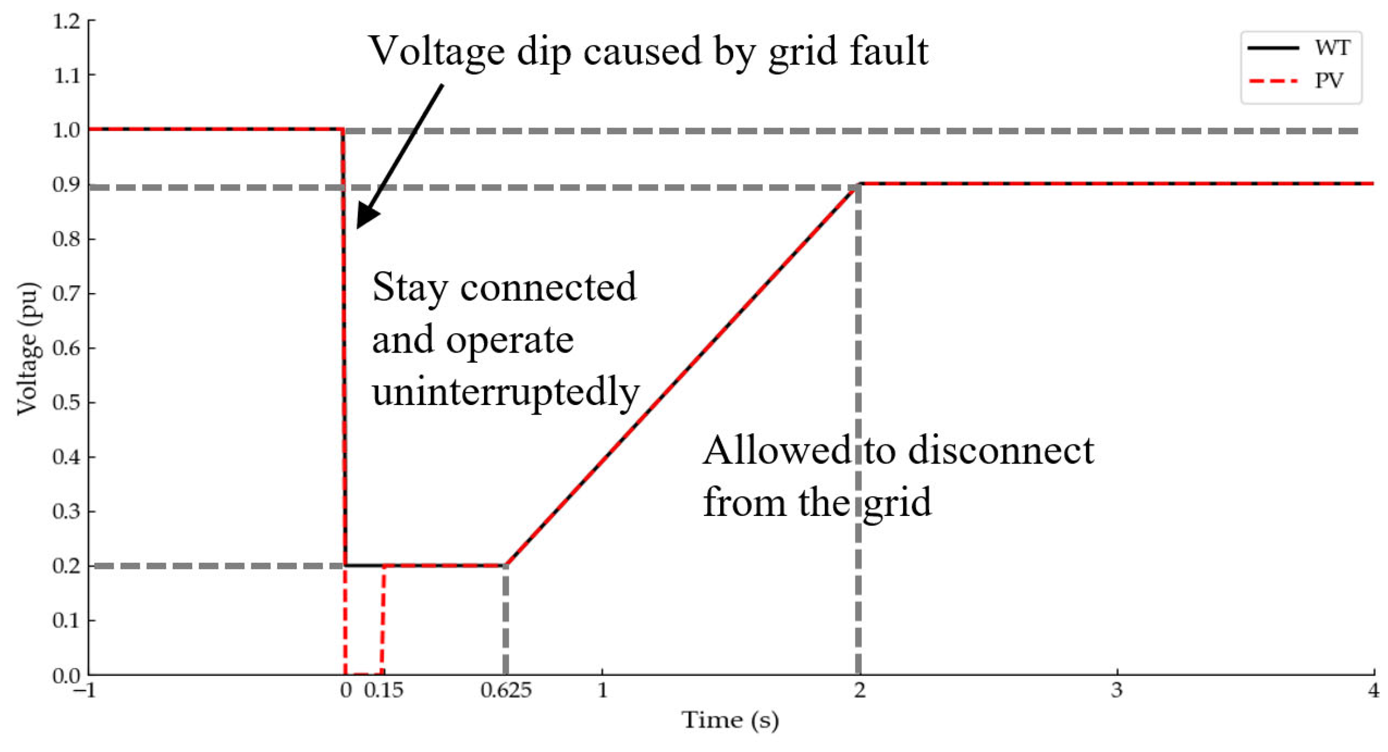
Figure 1. LVRT requirements for renewable energy in China.
Processes 14 00120 g001
Figure 2. Transient response of renewable energy units during LVRT after the short-circuit fault.
Processes 14 00120 g002
Figure 3. Transient response of renewable energy units tripping after the short-circuit fault: (a) WF tripping characteristics curve; (b) PV tripping characteristics curve.
Processes 14 00120 g003
Figure 4. Characteristics curve of the VDCOL function.
Processes 14 00120 g004
Figure 5. Transient response curve of DC after the short-circuit fault.
Processes 14 00120 g005
Figure 6. Directed weighted graph of the fault transient evolution process.
Processes 14 00120 g006
Figure 7. Flowchart of fault evolution scenario generation.
Processes 14 00120 g007
Figure 8. The change curve of renewable energy active power over time during LVRT.
Processes 14 00120 g008
Figure 9. The change curve of renewable energy active power over time during tripping: (a) WF tripping active power change curve; (b) PV tripping active power change curve.
Processes 14 00120 g009
Figure 10. The change curve of DC power over time during CF.
Processes 14 00120 g010
Figure 11. Structural diagram of the 500 kV AC lines and DC lines in the provincial power grid.
Processes 14 00120 g011
Figure 12. SHAP value of the renewable energy LVRT state transition model.
Processes 14 00120 g012
Figure 13. Features analysis based on SHAP: (a) SHAP value of the renewable energy LVRT T1 model; (b) importance ranking of input features for the DC CF T1 model.
Processes 14 00120 g013
Figure 14. SHAP value of the WF LVRT T2 model.
Processes 14 00120 g014
Figure 15. SHAP value of the PV LVRT T2 model.
Processes 14 00120 g015
Table 1. Input feature set for state transition and temporal feature T1 models.
Feature NameSymbolFeature Description
Fault grounding impedancezfFault information
Fault durationT0
Mutual impedance between the equipment bus and the fault busRif + jXif
Equivalent impedance at the fault busRff + jXffGrid strength
Equivalent impedance at the equipment busRii + jXii
Pre-fault steady-state voltage at the fault busUf0Grid operating condition
Pre-fault steady-state voltage at the renewable energy and DC busUi0
Table 2. Input feature set for temporal feature T2 models.
Feature NameSymbolFeature Description
Generator bus self-impedanceRgg + jXggSupporting capability of the equipment’s adjacent area
Mutual impedance between equipment and near-area busRib + jXib
Multiple renewable energy stations short-circuit ratioMRSCRi
Active current coefficient
during LVRT
kp1Renewable energy LVRT related control coefficients
Reactive current coefficient
during LVRT
kq1
Active current coefficient
during LVRT recovery
kp2
Table 3. Performance metrics of state transition models.
State Transition ModelsMachine Learning ModelAcc (%)Pre (%)Re (%)F1 (%)Time (s)
LVRTLogistic regression96.04%94.53%95.63%95.08%0.326
Neural network97.33%95.10%98.39%96.72%3.058
SVM96.51%95.14%96.20%95.67%5.230
XGBoost99.36%98.63%99.78%99.20%1.839
WF TrippingLogistic regression99.18%98.21%100%99.10%0.003
PV TrippingLogistic regression98.80%98.18%99.08%98.63%0.002
CFLogistic regression99.04%97.00%99.44%98.17%0.009
Table 4. Performance metrics of temporal feature models.
Temporal Feature ModelsMachine Learning ModelRMSE (ms)MAE (ms)R2Time (s)
LVRT T1Linear regression18.8210.140.110.004
Neural network8.823.600.805.449
SVM12.694.170.599.462
XGBoost4.520.850.950.844
WT LVRT T2Linear regression42.8029.340.530.006
Neural network19.929.930.904.012
SVM19.2010.880.910.634
XGBoost6.822.210.990.355
PV LVRT T2Linear regression41.5227.220.480.041
Neural network22.8412.220.8410.054
SVM25.7417.810.807.674
XGBoost8.413.150.981.311
CF T1Linear regression33.2024.260.370.002
Neural network22.2212.900.720.282
SVM10.187.740.940.117
XGBoost7.543.170.970.148
Table 5. LVRT risk assessment key parameters.
Renewable Energy StationPlvrt0 (MW)kp1T0 (s)T1 (s)T2 (s)T3 (s)
PV 21130840.10.100.11.565
PV 2108586.540.30.10.0150.0850.67
WF 2117176.720.40.120.010.0051.07
WF 21306910.20.1800.181.57
Table 6. Renewable energy LVRT risk assessment result.
Renewable Energy StationRlvrt1
(MW)
Rlvrt2
(MW)
Rlvrt3
(MW)
Rlvrt
(MW)
Rlvrt,sim
(MW)
Absolute Difference (MW)Relative Error
(%)
PV 2113000.845.9166.7566.7070.0490.73
PV 2108500.5372.0292.5662.3950.1717.14
WF 2117100.2702.2212.4912.5990.1084.16
WF 2130601.6385.7157.3537.2160.1371.90
Table 7. Renewable energy tripping risk assessment result.
Renewable Energy StationPoff0
(MW)
T0
(s)
Roff1
(MW)
Roff
(MW)
Roff,sim
(MW)
Absolute Difference (MW)Relative Error
(%)
WF 21304910.150.9191.9191.9560.0460.05%
WF 21306910.180.9191.9191.9560.0460.05%
PV 21300560.21.1257.1256.9830.1370.24%
Table 8. DC CF risk assessment result.
DCPcf0
(MW)
T0
(s)
T1
(s)
T2
(s)
T3
(s)
tv3
(s)
Rcf1
(MW)
Rcf2
(MW)
Rcf3
(MW)
Rcf
(MW)
Rcf,sim
(MW)
Absolute Difference (MW)Relative Error
(%)
(124,119)1274.970.1500.22.2553.2025.499171.497196.997195.9461.0510.54%
(45,50)1856.250.10.090.0233.957037.125332.914370.039373.8723.8331.03%
Table 9. Prediction and risk assessment results of renewable energy LVRT under initial fault 1.
Evaluation DimensionEvaluation MetricValue
Fault identification resultsAcc (%)98.25%
Re (%)100%
Pre (%)98.25%
Temporal parameter prediction resultsRMSE T1 (s)0.0044
MAE T1 (s)0.0014
RMSE WF-T2 (s)0.0248
MAE WF-T2 (s)0.0225
RMSE PV-T2 (s)0.0180
MAE PV-T2 (s)0.0159
Risk assessmentAbsolute Difference (MW)2.992
Relative Error (%)1.08%
Table 10. Comparison of fault evolution path prediction and simulation results under initial fault 2.
Renewable Energy StationFault Prediction ResultLVRT
T1 Prediction
Result (s)
LVRT
T2 Prediction
Result (s)
Simulation Result
WF 21227Tripping————1.1 s tripping
WF 21228Tripping————1.1 s tripping
WF 21238LVRT00.141 s LVRT, 1.14 s enters recovery state, 1.99 s enters normal operation state
WF 21239LVRT00.141 s LVRT, 1.14 s enters recovery state, 2.2 s enters normal operation state
PV 21125LVRT00.141 s LVRT, 1.14 s enters recovery state, 2.265 s enters normal operation state
PV 21139LVRT00.141 s LVRT, 1.14 s enters recovery state, 2.735 s enters normal operation state
"——" in the table indicates that the corresponding entry is not applicable or does not exist in the given case, and therefore no value is required.
Table 11. Risk assessment result under initial fault 2.
Renewable Energy StationRoff
(MW)
Rlvrt
(MW)
Roff,sim
(MW)
Rlvrt,sim
(MW)
Absolute Difference (MW)Relative
Error
(%)
WF 2122770.7——70.735——0.0350.05%
WF 2122870.7——70.735——0.0350.05%
WF 21238——2.233——2.4330.28.22%
WF 21239——5.451——5.9010.457.63%
PV 21125——6.195——6.1360.0590.96%
PV 21139——4.809——4.6220.1874.05%
total141.418.688141.4719.0920.4740.30%
Disclaimer/Publisher’s Note: The statements, opinions and data contained in all publications are solely those of the individual author(s) and contributor(s) and not of MDPI and/or the editor(s). MDPI and/or the editor(s) disclaim responsibility for any injury to people or property resulting from any ideas, methods, instructions or products referred to in the content.