Article

Use of Cedrela odorata L. as a Biomaterial for Dye Adsorption in Wastewater: Simulation and Machine Learning Approaches for Scale-Up Analysis

by
Candelaria Tejada-Tovar
1,
Ángel Villabona-Ortíz
1,
Oscar E. Coronado-Hernández
2,
Modesto Pérez-Sánchez
3,* and
María Hueto-Polo
1
1
Process Design and Biomass Utilisation Research Group (IDAB), Chemical Engineering Department, Universidad de Cartagena, Avenida del Consulado St. 30, Cartagena de Indias 130015, Colombia
2
Instituto de Hidráulica y Saneamiento Ambiental, Universidad de Cartagena, Cartagena de Indias 130001, Colombia
3
Hydraulic and Environmental Engineering Department, Universitat Politècnica de València, 46022 Valencia, Spain
*
Author to whom correspondence should be addressed.
Processes 2025, 13(9), 2907; https://doi.org/10.3390/pr13092907
Submission received: 21 July 2025 / Revised: 3 September 2025 / Accepted: 10 September 2025 / Published: 11 September 2025
(This article belongs to the Special Issue Modeling and Optimization for Multi-scale Integration)

Abstract

Methylene blue and safranin are dyes that may have harmful effects on both aquatic ecosystems and human health. This research aims to simulate an industrial-scale operational adsorption column for competitively removing these dyes from wastewater, employing Cedrela odorata L. as a bioadsorbent material. Aspen Adsorption (v.1) software simulated an industrial-scale packed-bed adsorption column under various configurations. Moreover, machine learning algorithms were applied to predict the results generated by Aspen, representing an advancement in the development of new strategies in this field. The kinetic model employed was the Linear Driving Force (LDF) model. Adsorption efficiencies of 96.1% were achieved for both methylene blue and safranin using the Langmuir–LDF model. The Freundlich–LDF model showed efficiencies of 94.8% for methylene blue and 96% for safranin. Meanwhile, the Langmuir–Freundlich–LDF model achieved up to 96.1% for methylene blue and 94.8% for safranin. This study demonstrated the feasibility of simulating the competitive adsorption of dyes in solution at an industrial scale using Cedrela odorata L. as a bioadsorbent. The application of LDF kinetic models and adsorption isotherms (Langmuir, Freundlich, and Langmuir–Freundlich) resulted in high adsorption efficiencies, highlighting the potential of this approach for the remediation of dye-contaminated effluents as a viable method for predicting the performance of full-scale packed columns. Machine learning algorithms were implemented in this research, obtaining R2 higher than 0.996 for validation and testing stages for the responses of the model.

1. Introduction

Water pollution represents a significant challenge for humanity. In all environments, freshwater is vital for the survival of living organisms; however, industrial development has led to increasing contamination due to the discharge of substantial volumes of wastewater into lentic and lotic hydrosystems [1]. Such effluents often result from processes involving various toxic substances, such as dyes, which, upon entering freshwater systems, pollute both surface and groundwater. The latter, in particular, constitutes a vital source of water for domestic and agricultural use [2].
Dyes are compounds that exhibit high resistance to degradation due to their considerable thermal stability, and are also highly toxic to ecosystems. They are widely used across various industrial sectors, including food, cosmetics, automotive, pharmaceuticals, plastics, paints, leather, and textiles [3]. These pollutants can pose severe health risks due to their toxicity, including skin and eye irritation. They may even contribute to genetic mutations and cancer [4].
The removal of dyes for this kind of water has therefore become a significant environmental concern. Various treatment techniques have been developed to remove such contaminants from hydrosystems. Among these are coagulation/flocculation, which uses either chemical or natural agents to destabilise and aggregate suspended particles in water, thereby facilitating their removal [5]. Another technique is electrocoagulation, an advanced water treatment method that destabilises and aggregates suspended, emulsified, or dissolved pollutants through the application of a low-voltage direct current across sacrificial electrodes—commonly made of aluminium or iron [6].
Among these methods, adsorption stands out as a surface phenomenon in which adsorbates are transferred to the surface of adsorbents. This technique is widely employed due to its flexibility, cost-effectiveness, and broad applicability [7]. The adsorption process starts when the contaminated solution carries adsorbate molecules to the boundary layer of the adsorbent. These molecules then diffuse from the boundary layer to the external surface and subsequently into the internal pore structure, where active adsorption sites capture the contaminant ions [8]. Adsorption can be classified as either physical (physisorption) or chemical (chemisorption). Physisorption is governed by weak, short-range electrostatic forces such as Van der Waals interactions, resulting in relatively weak binding. In contrast, chemisorption involves the formation of chemical bonds between the adsorbate and the adsorbent, resulting in more substantial and specific interactions that are more energy-intensive and difficult to reverse [9].
Various low-cost adsorbents derived from lignocellulosic biomass—particularly agricultural residues such as rice husks [10], sugarcane bagasse [11], and banana peels [12]—have been widely used in both raw and modified forms for contaminant removal from wastewater. These studies have highlighted the need for further research and development of biomass-based composite columns for potential industrial-scale applications. However, most investigations remain limited to laboratory-scale experiments. As a result, efforts have been made to predict the behaviour of adsorption processes at larger scales through computational modelling. To this end, tools such as Aspen Adsorption—a software developed by AspenTech—have been employed to simulate adsorption processes under various conditions. The primary objective of these simulations is to predict and understand the performance of contaminant removal from aqueous solutions at larger scales.
Although advances have been reported in the use of different new materials as packing in adsorption columns, there are still significant gaps in our understanding of how they operate when scaled up to full scale, especially under typical industrial process operating conditions. Few studies evaluate the performance of these columns in competitive adsorption situations, in which multiple contaminants coexist and compete for active adsorption sites. Additionally, using simulation tools such as Aspen Adsorption to model systems with various contaminants represents a significant challenge, as there are very few studies in the literature that address complex contamination matrices. In this work, a binary contaminant system was addressed as a starting point; however, the challenge remains to develop future studies in which more than two contaminants and different types of molecules coexist, such as mixtures that include two dyes, two metals, or other compounds present in water, which would allow for a closer approximation to real and highly complex scenarios.
On the other hand, current trends indicate that the implementation of digital twin models in water treatment plants can support planners in making decisions more rapidly compared to traditional software, which typically requires specialised personnel to simulate processes [13,14]. The implementation of digital twin models in water treatment contributes to the development of reliable systems that support rapid decision-making, in contrast to traditional approaches. In this context, the integration of machine learning algorithms enables faster and more efficient responses, as they can reproduce the behaviour of mathematical models without the need to run complex software or solve computationally demanding equations. Machine learning (ML) algorithms reduce computational time and can be used for predictive analysis and operational optimisation [15].
The integration of Aspen Adsorption with digital twin technology, in combination with ML algorithms, offers several advantages for the modelling, simulation, and optimisation of adsorption processes used to remove contaminants from water bodies. This approach enables the prediction of equipment performance by developing models that forecast column behaviour with greater accuracy and reduced computational time. Moreover, digital twins can be trained with new input data derived from software simulations, thereby facilitating the prediction or validation of key parameters such as rupture time (RT), saturation time (ST), and overall process efficiency. This, in turn, supports more informed and precise operational decision-making [16].
Therefore, the present study aims to model an industrial-scale compact bed adsorption column using advanced computational tools, applying a comprehensive parametric analysis together with machine learning algorithms to optimise the process of removing methylene blue and safranin from aqueous solutions, using Cedrela odorata L. sawdust waste as the adsorbent material. This research seeks to demonstrate the potential of computational tools, combined with machine learning algorithms, to predict the performance of adsorption columns with high accuracy. It also provides quantitative and validated information for the upscaling of a fixed-bed column using Cedrela odorata L. waste as an adsorbent material, thus optimising its design and operation at an industrial level.

2. Materials and Methods

Figure 1a presents the methodology employed in this study, which integrates simulations using Aspen Adsorption with ML techniques. Two contaminants were considered: methylene blue and safranin. The proposed methodology is suitable for interpreting efficiency (1 − Cf/C0), saturation time, and rupture time.
The methodology begins by identifying the target contaminants for removal—in this case, the previously mentioned dyes. Subsequently, various parameters required by Aspen Adsorption were defined, including column diameter, mass transfer coefficient, void porosity, total porosity, and the constants associated with the selected isotherm models, namely Langmuir and Freundlich. To assess column performance, two independent variables were selected for sensitivity analysis: inlet flow rate and bed height. Simulations were then carried out, producing results related to process efficiency, ST, and RT. Finally, several ML algorithms were implemented to simulate the obtained responses.
To perform the modelling of a packed adsorption column using agro-industrial residues for the removal of dyes in solution with the Aspen Adsorption software, it is first necessary to define the chemical components to be removed together with the thermodynamic package (see Figure 1b). For this purpose, the option “Configure Properties” is selected, followed by access to the “Aspen Property System” section, where “Edit using Aspen Properties” is chosen. In this section, the contaminants to be removed—namely methylene blue and safranine—are specified, as well as the thermodynamic package to be employed, in this case UNIQUAC. Subsequently, the construction of the packed adsorption column system is carried out by employing the library and the various tools integrated within Aspen Adsorption. To this end, “Libraries” is accessed, “Adsim” is selected, and the “Liquid” option is chosen. Within this section, the different components required to configure the adsorption system are defined, including the packed bed and the feed and product streams. The following step involves specifying the parameters and criteria for configuring the adsorption column, the inlet and outlet streams, the governing mathematical equations, and other relevant variables. This requires setting up the key sections that ensure proper definition of the simulation parameters, namely “General”, “Mass/Momentum Balance”, “Kinetic Model”, “Isotherm Model”, and “Energy Balance”. Numerical values are then assigned to a range of parameters associated with both the feed and product streams, such as flow rate, contaminant concentration, temperature, and pressure. Additional parameters include column height and diameter, mass transfer coefficient, void porosity, total porosity, and the main coefficients related to the selected mathematical models. Once these inputs are established, a graphical representation of the adsorption process behaviour over time is generated. This is accomplished by accessing the “Flows Plot: Flowsheet” section, selecting “Add Form”, choosing the “Plot” option, assigning a name to the graph, and specifying the parameters to be displayed. Finally, the operational state of the adsorption process is defined—in this case “Dynamic State”—and the simulation is executed, thereby obtaining the rupture curve that characterises the behaviour of the adsorption system.

2.1. Adsorption Column Configuration

To simulate the packed-bed column for the adsorption of methylene blue and safranin, it is first necessary to define the thermodynamic package used to calculate the physicochemical properties of the liquid phase. These properties are essential for properly characterising the solution interacting with the adsorbent material—that is, the fluid entering the column in contact with the selected adsorbent [17].
For this study, the UNIQUAC (Universal Quasi-Chemical) method was employed to determine the physical properties of the feed stream in the adsorption column. The choice of this method is justified by its capability to describe liquid systems containing complex organic solutes dissolved in water, while considering molecular interactions between the contaminant species present [18].
Following the selection of the thermodynamic model, the adsorption column must be configured in Aspen Adsorption, which includes several key sections required to define the simulation parameters correctly. These sections are: General, Mass/Momentum Balance, Kinetic Model, Isotherm Model, and Energy Balance. The considerations made for each section are detailed in the following subsections.

2.1.1. General Section

This section presents the discretisation method used to simulate the adsorption process. For this study, the first-order upwind differentiation scheme 1 (UDS1) was implemented. This numerical method, widely used to solve mass transport equations, is based on a first-order Taylor series expansion, which allows for a stable and efficient formulation for the approximation of convective terms [19]. The process is expressed by Equation (1):
δ Γ i δ z = Γ i Γ i 1 Δ z
Additionally, the simulation was configured with a total of 10 discretisation nodes across the adsorption bed.

2.1.2. Mass/Momentum Balance Section

This section outlines the fundamental assumptions regarding axial dispersion in the liquid phase, the treatment of pressure drop in the adsorption column model, and whether the velocity remains constant or varies along the column. In this study, no pressure drop was assumed. The simulation of the packed-bed adsorption column for dye removal considered convection as the sole transport mechanism. Accordingly, the solute is transported along the bed exclusively by the bulk flow of the fluid, and the velocity is assumed to remain constant throughout the column [20].

2.1.3. Kinetic Model Section

In this section, the user establishes which kinetic model will define how to explain the rate at which the adsorption process occurs. In this case, among the different models that Aspen Adsorption V10 handles, the Linear Driving Force (LDF) model was selected, which assumes that a driving force influenced by concentration affects mass transfer, describing the rate at which the contaminant is adsorbed onto the solid phase [21]. The model is expressed by Equation (2):
w k t =   M T C s k w k * w k

2.1.4. Isotherm Model Section

This section defines the isothermal model used to describe the interactions between the adsorbate and the adsorbent. Table 1 shows the different isothermal models selected for this study.
Table 1. Selected Isotherm Models for the Simulation of the Adsorption Column.
DefinitionEquationObservationReference
Langmuir isotherm model q e = q m a x b C e 1 + b C e           ( 3 ) q e : Adsorption capacity of the contaminant at equilibrium.
q m a x : Maximum loading capacity of the adsorbent.
b :   Langmuir constant.
C e : Equilibrium concentration of the contaminant in solution.
[22,23]
Freundlich isotherm model q e = k f C e 1 / n             ( 4 ) q e : Adsorption capacity of the contaminant at equilibrium.
k f : Freundlich constant.
C e : Equilibrium concentration of the contaminant in solution.
1 / n : Reflects the influence of the initial concentration on the adsorption capacity.
[24,25]
Langmuir–Freundlich isotherm model q e = q m a x K C e n 1 + K C e n             ( 5 ) q e : Adsorption capacity of the contaminant at equilibrium.
q m a x : Maximum adsorption capacity.
C e :   Equilibrium concentration of the contaminant in solution.
K : Affinity or adsorption energy constant.
n : Surface heterogeneity factor.
[26,27].

2.1.5. Energy Balance Section

This section defines how the energy balance is addressed in the adsorption model. In this study, isothermal operating conditions were assumed. That is, the temperature of the system was considered to remain constant throughout the entire adsorption process.

2.2. Parameters Required for the Parametric Sensitivity Analysis

To assess the scale-up simulation of the adsorption column for methylene blue and safranin using Aspen Adsorption, it is necessary to examine the effect of various operating conditions that may influence the adsorption process and its overall performance. Therefore, a parametric sensitivity analysis was conducted on several key variables [20].
In this study, the bed height and inlet flow rate were selected as the primary variables for evaluation, while maintaining a constant initial concentration of 2000 mg/L for both methylene blue and safranin, an operating pressure of 1 atm, and a temperature of 30 °C. By modifying these parameters, the system’s response under different operating conditions can be observed, helping to identify which variable has the most significant impact on adsorption efficiency. Table 2 presents the ranges of the evaluated parameters considered in the parametric study.
In addition, the Aspen Adsorption V10 software requires several other parameters for the proper modelling and sizing of the adsorption column. These variables are essential during the simulation of the packed-bed adsorption column filled with cedarwood sawdust, which is used for the removal of dyes from aqueous solution—specifically, methylene blue and safranin in this case.
Key parameters include the bulk density of the biomaterial, the column diameter, the mass transfer coefficient, the void fraction, and the total porosity. Additionally, the values of the constants corresponding to the selected isotherm models are required. These parameters are presented in Table 3. The values related to the adsorbent were obtained mainly from previous research carried out by our research group and scientific literature, where cedar sawdust residues were evaluated as a biomaterial in adsorption processes. In the case of parameters not directly associated with the properties of the bioadsorbent, such as those related to the sizing and design of the column, values reported in adsorption column simulation studies were adopted and adjusted for application in Aspen Adsorption. These parameters were scaled to industrial conditions following the criteria of geometric and hydrodynamic similarity.
However, it should be noted that different criteria, such as the origin of the waste, particle size, moisture content, pre-treatments applied, and equipment sizing taken from the reference studies, may introduce biases in the estimation of adsorption capacity and kinetics, as well as in the simulation process.

2.3. Machine Learning Techniques

In this study, 28 ML algorithms were applied to digitalise the simulations. The MLAs were trained on a dataset comprising 54 entries related to dye removal, using the Freundlich–LDF, Langmuir–LDF, and Langmuir–Freundlich–LDF models. For all simulations, the predictors included the type of contaminant, bed height, inflow rate, and the model type. The ML algorithms were executed considering three different types of responses: 1 − Cf/C0, ST, and RT. Figure 2 illustrates the relationships among the predictors employed in this study. A five-fold cross-validation scheme was implemented to assess model performance. Additionally, 25% of the data were set aside for testing purposes during the simulation process.
The 28 ML algorithms employed in this study are listed in Table 4, where they are identified in parentheses. All simulations were performed using MATLAB R2024b, utilising the algorithms available through the Regression Learner App. This tool facilitates the identification of the most suitable algorithm for modelling the processes under analysis.
For selecting the ML algorithms for the three analysed responses, the following statistical measures were used. The Root Mean Square Error (RMSE) is calculated by:
R M S E = 1 N i = 1 N ( T i P i ) 2
where N = total number of observations, T i = true value of a response, and P i = predicted value of a response.
The coefficient of determination or R-squared (R2) is given by:
R 2 = 1 i = 1 N ( T i P i ) 2 i = 1 N ( T i T ¯ ) 2
where T ¯ = average value of observations.
The selection of ML algorithms is based on the model exhibiting the lowest RMSE value and the highest R-Squared value, ideally approaching 1.
In this research, two ML algorithms were used since the best fit of validation and testing phases was achieved considering the RMSE and R-squared.
In this sense, the Gaussian Process Regression is a probabilistic model that follows a Gaussian distribution [32].
P ( y f , X ) ~ N ( y H β + f , σ 2 I )
where y = response variable, f = latent variable introduced in each observation, X = predictors, H = matrix of basis functions, β = coefficient computed from the dataset, and I = identity matrix, and σ 2 = error variance.
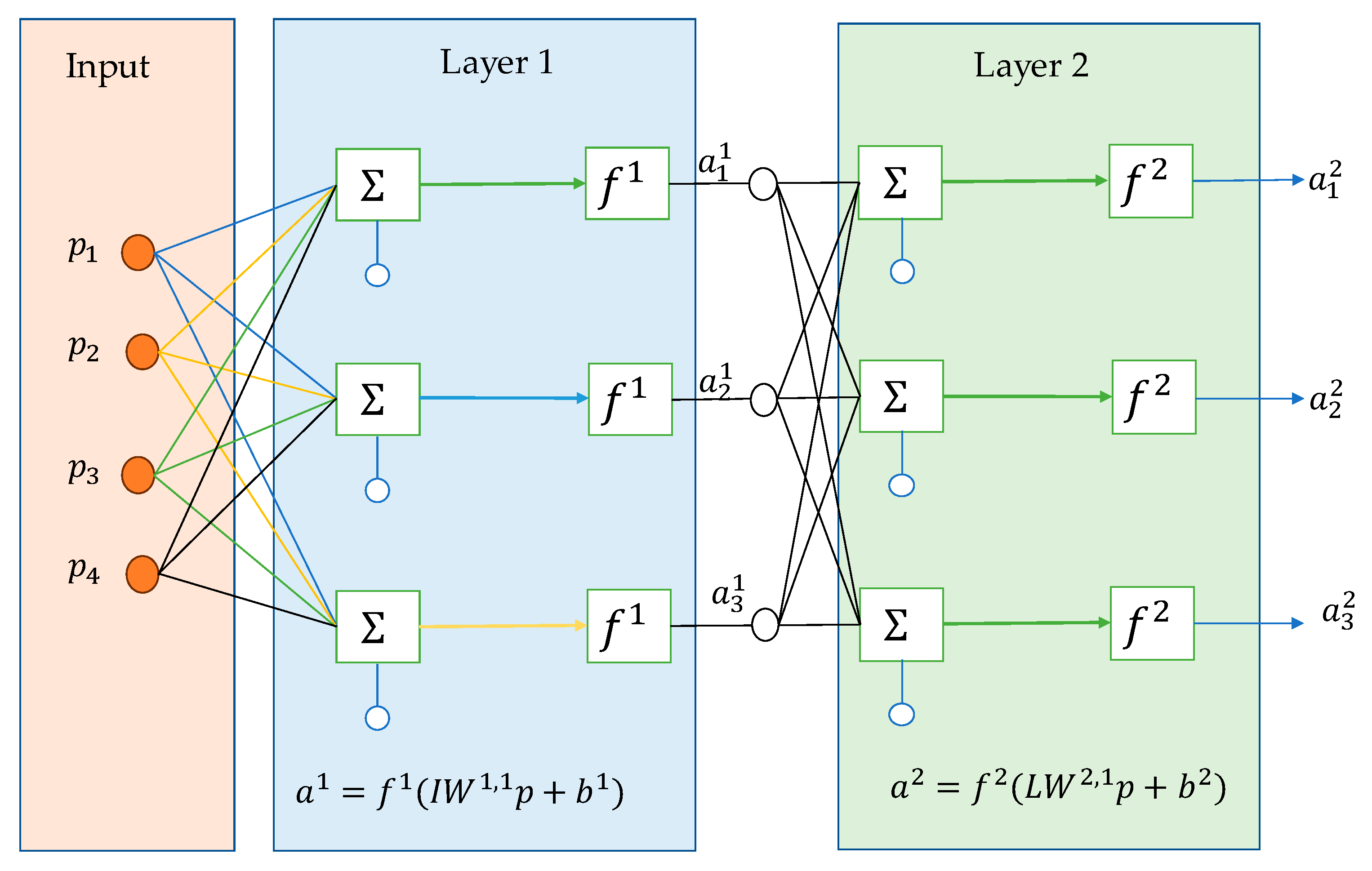
The bilayered neural networks provided the best fit for the RT and ST. This ML algorithm employs two layers, as shown in Figure 3 [35,36]. The output vector can be computed as follows:
a 2 = f 2 { L W 2 , 1 f 1 I W 1 , 1 p + b 1 + b 2 }
where p = input vector, a = output vector, W = weight matrix, b =   bias vector, I W = input weight matrix, and L W = layer weight matrix. Superscripts 1 and 2 denote the first and second layers, respectively.

3. Results and Discussion

3.1. Aspen Adsorption Simulation

Using Aspen Adsorption software, multiple simulations were performed for the expanded adsorption column to remove methylene blue and safranin from water. These simulations were performed with different configurations of the parameters selected for the sensitivity study, which allowed key parameters to be obtained: the rupture time, the time at which the adsorbent begins to lose its removal capacity; the saturation time, when the adsorbent stops removing the contaminant; and the adsorption efficiency, reflecting the efficiency of material in the process.
These simulations were performed utilising the selected isothermal models in conjunction with the chosen kinetic model.

3.2. Parametric Sensitivity Analysis

A parametric sensitivity analysis was conducted to identify the influence of key variables on the performance of the modelled system. In this study, bed height and inlet flow rate were selected as the primary parameters of interest.

3.2.1. Effect of Varying the Inlet Flow Rate

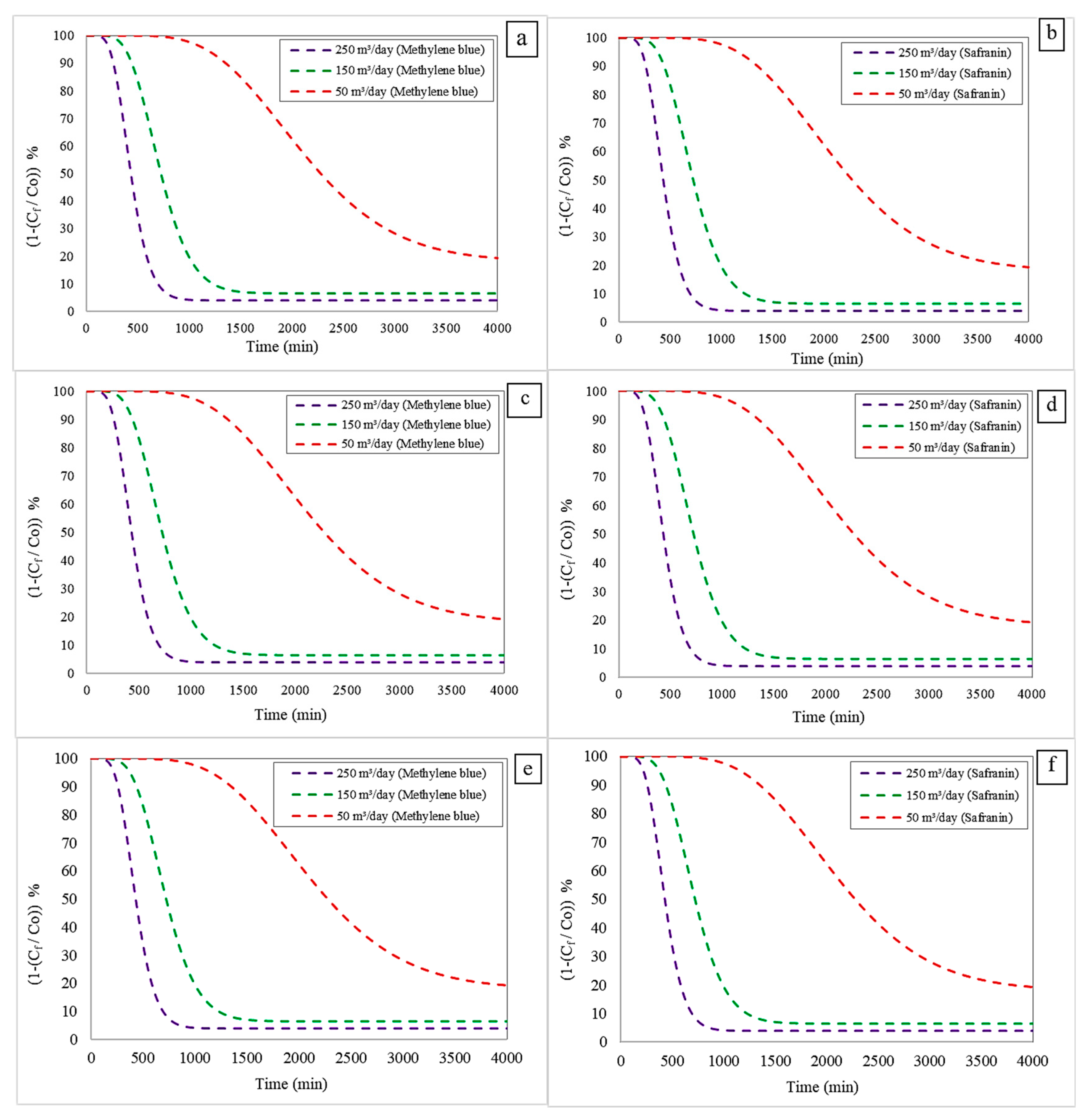
The performance of the adsorption column was evaluated by varying the inlet flow rate parameter. This alteration was carried out using values of 50, 150 and 250 m3/day, while maintaining a fixed column height of 3 m and an initial concentration of both dyes of 2000 mg/L. Figure 4 shows the removal of contaminant profiles for the different isothermal models that were selected in this study: Freundlich (Figure 4a,b), Langmuir (Figure 4c,d) and Langmuir–Freundlich (Figure 4e,f), which are combined with the Linear Driving Force (LDF) kinetic model.
It can be observed that, as the flow rate to the compact bed increases, the adsorption efficiency increases, but the RT and ST decrease. This behaviour is attributed to the increase in fluid flow velocity, which leads to faster saturation of the adsorbent pores and, consequently, a reduction in the contact time available for adsorption [30].
For the Freundlich–LDF model:
  • In the case of methylene blue, at 50 m3/day, the RT and ST were 241 min and 1430 min, respectively. When the flow rate was increased to 150 m3/day, these times decreased to 193 min and 1151 min. Further increasing the flow to 250 m3/day resulted in values of 141 min (RT) and 870 min (ST).
  • A similar trend was observed for safranin, with times of 241 min and 1430 min at 50 m3/day, decreasing to 193 min and 1151 min at 150 m3/day, and finally reaching 142 min and 870 min at 250 m3/day.
For the Langmuir–LDF model:
  • For methylene blue, the RT and ST at 50 m3/day were 246 min and 1439 min, respectively. These decreased to 195 min and 1158 min at 150 m3/day, and 142 min and 872 min at 250 m3/day.
  • The same behaviour was observed for safranin, with times of 241 min and 1430 min at 50 m3/day, reducing to 193 min and 1151 min at 150 m3/day, and 142 min and 870 min at 250 m3/day.
For the Langmuir–Freundlich–LDF model:
  • The results followed the same trend. For methylene blue, the RT and ST > were 241 min and 1430 min at 50 m3/day, decreasing to 193 min and 1151 min at 150 m3/day, and to 141 min and 870 min at 250 m3/day.
  • Similarly, for safranin, the times were 241 min and 1430 min at 50 m3/day, 193 min and 1151 min at 150 m3/day, and 142 min and 872 min at 250 m3/day.
The adsorption efficiencies for both methylene blue and safranin increased slightly with flow rate across all models: 94% at 50 m3/day, 95% at 150 m3/day, and 96% at 250 m3/day. These results suggest that all three isotherm–kinetic model combinations effectively describe the adsorption process under the conditions studied.

3.2.2. Effect of Changing the Column Height

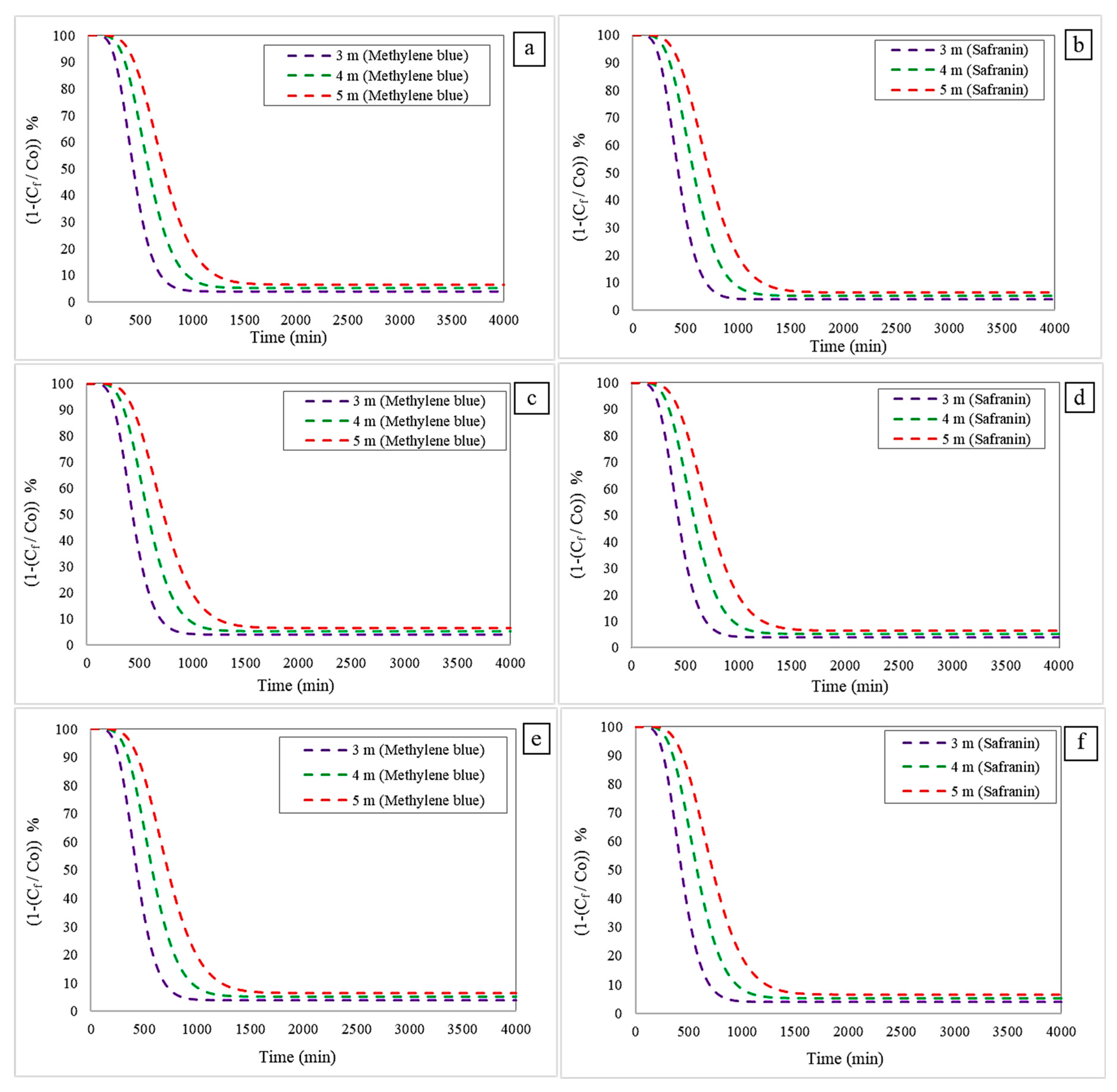
To evaluate the performance of the packed bed, a parametric alteration of the adsorption bed height was performed. In this study, a variation of this parameter in a range of 3, 4 and 5 m was used, keeping the initial pollutant concentration and the inlet flow rate constant at 2000 mg/L and 250 m3/day, respectively. Figure 5 shows the removal of contaminant profiles of the Freundlich (Figure 5a,b), Langmuir (Figure 5c,d) and Langmuir–Freundlich (Figure 5e,f) isotherm models, each coupled to the LDF kinetic model. The behaviour shows that an increase in height leads to longer rupture and saturation times, accompanied by a reduction in the overall efficiency of the process. This performance can be explained by increased adsorbent material, which offers a greater number of active sites and delays their occupation, thereby prolonging the total adsorption time [37]. Simulation data confirmed this behaviour for both dyes, obtaining:
  • Freundlich–LDF model: For methylene blue removal, a bed height of 3 m resulted in RT and ST values of 145 min and 870 min, respectively. Increasing the height to 4 m extended these times to 244 min (RT) and 1430 min (ST). At 5 m, the values rose further to 760 min (RT) and 4183 min (ST). The same trend was observed for safranin removal: at 3 m, RT and ST were 142 min and 870 min; at 4 m, these increased to 244 min and 1430 min; and at 5 m, they reached 761 min and 4183 min, respectively.
  • Langmuir–LDF model: A similar pattern was found. For methylene blue, a bed height of 3 m resulted in 142 min (RT) and 872 min (ST); increasing the height to 4 m led to 244 min and 1436 min, while at 5 m, the values were 760 min and 4215 min. For safranin, RT and ST at 3 m were 142 min and 870 min; at 4 m, they increased to 244 min and 1430 min; and at 5 m, to 761 min and 4183 min.
  • Langmuir–Freundlich–LDF model: This model exhibited the same behaviour. For methylene blue, the RT and ST at 3 m were 141 min and 870 min, respectively. At 4 m, values rose to 244 min and 1430 min, and at 5 m, to 760 min and 4183 min. For safranin, at 3 m the times were 142 min (RT) and 872 min (ST); at 4 m, 244 min and 1430 min; and 5 m, 761 min and 4183 min.
In all models, adsorption efficiencies for methylene blue and safranin were 94% at 3 m, 95% at 4 m, and 96% at 5 m. These results suggest that all three isotherm–kinetic model combinations are capable of accurately representing the adsorption process under the tested conditions.
As can be seen in Figure 4 and Figure 5, the similar behaviour in the RT and ST values obtained during the simulation of the adsorption process of the two dyes studied can be attributed to different factors. On the one hand, both dyes are cationic compounds with similar molecular mass and aromatic structure with amino groups, which gives them similar molecular dimensions and mechanisms of interaction with the adsorbent, favouring similar kinetics and adsorption capacities. On the other hand, the simulation conditions in Aspen Adsorption used similar mass transfer parameters and mathematical models that do not incorporate significant differences in ionic competition, surface heterogeneity, or specific hydrodynamic effects for each dye, which reduces the sensitivity of the model to molecular variations and leads to very similar RT and ST predictions for both contaminants.

3.3. Machine Learning Implementations

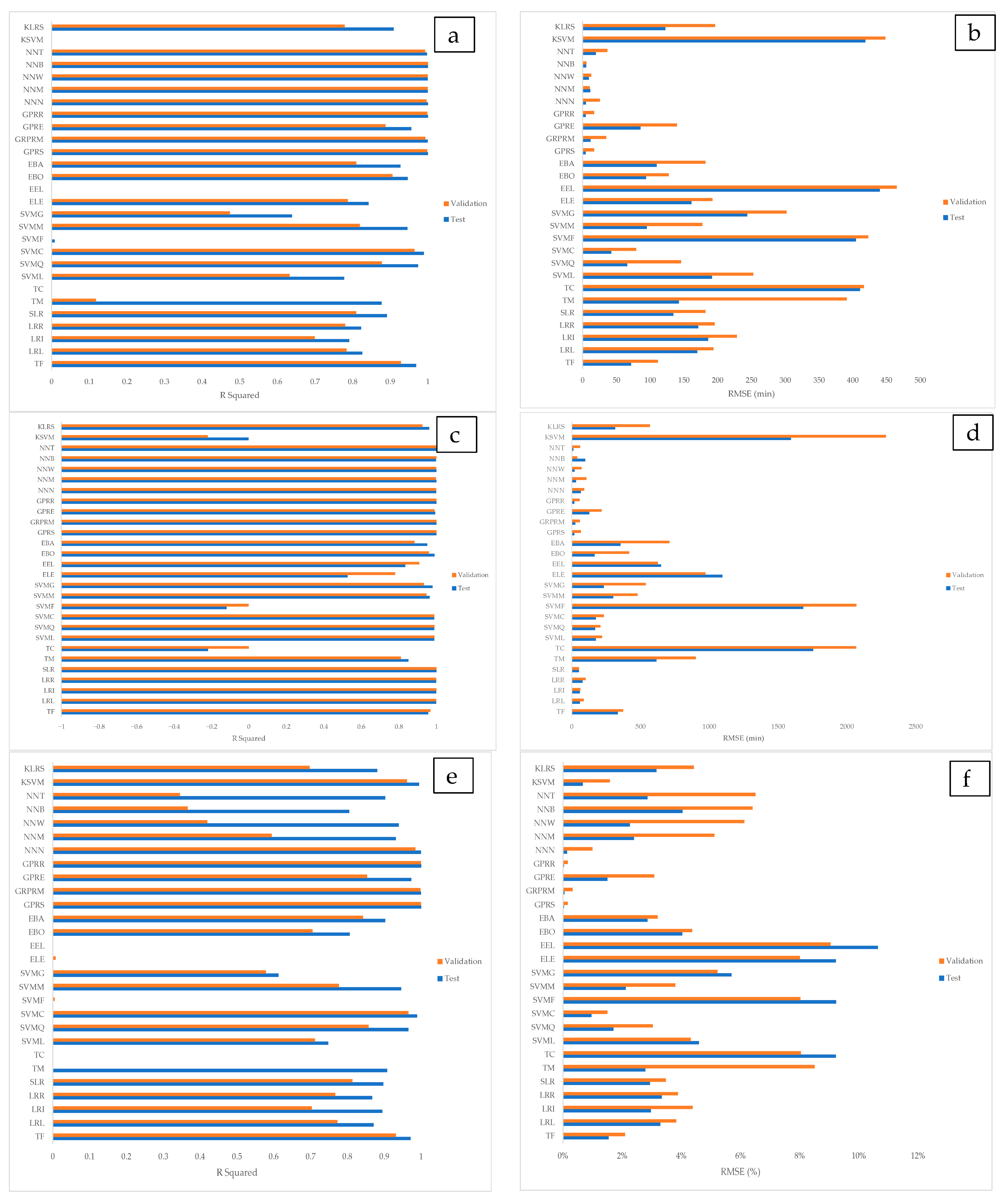
To digitalise the responses provided by the Aspen adsorption model, 28 ML algorithms (see Table 4) were applied to identify the most suitable models for ST, RT, and 1 C f / C 0 . Figure 6 presents the statistical performance metrics (RMSE and R-squared) for the ML algorithms. These metrics were calculated for both the validation and testing stages to avoid model overfitting.
According to the results, the Gaussian Process Regression model with a Rational Quadratic kernel (Rational Quadratic GPR) provided the best fit for both validation and testing stages in terms of efficiency ( 1 C f / C 0 ), achieving an R-squared value of 0.999. In terms of RMSE, values of 0.16 for validation and 0.03% for testing were obtained.
The bilayered neural network was selected to model both ST and RT, as it yielded the best results for RMSE and R-squared. Table 5 summarises the selected ML algorithms. According to the results, the selected ML models required training times ranging from 1.81 to 3.64 s, which is highly advantageous as simulations can be performed rapidly. Moreover, Aspen software requires a licence to run simulations. In this regard, engineers can implement ML models for contaminant modelling, thereby reducing simulation time and avoiding the need for commercial licenses.
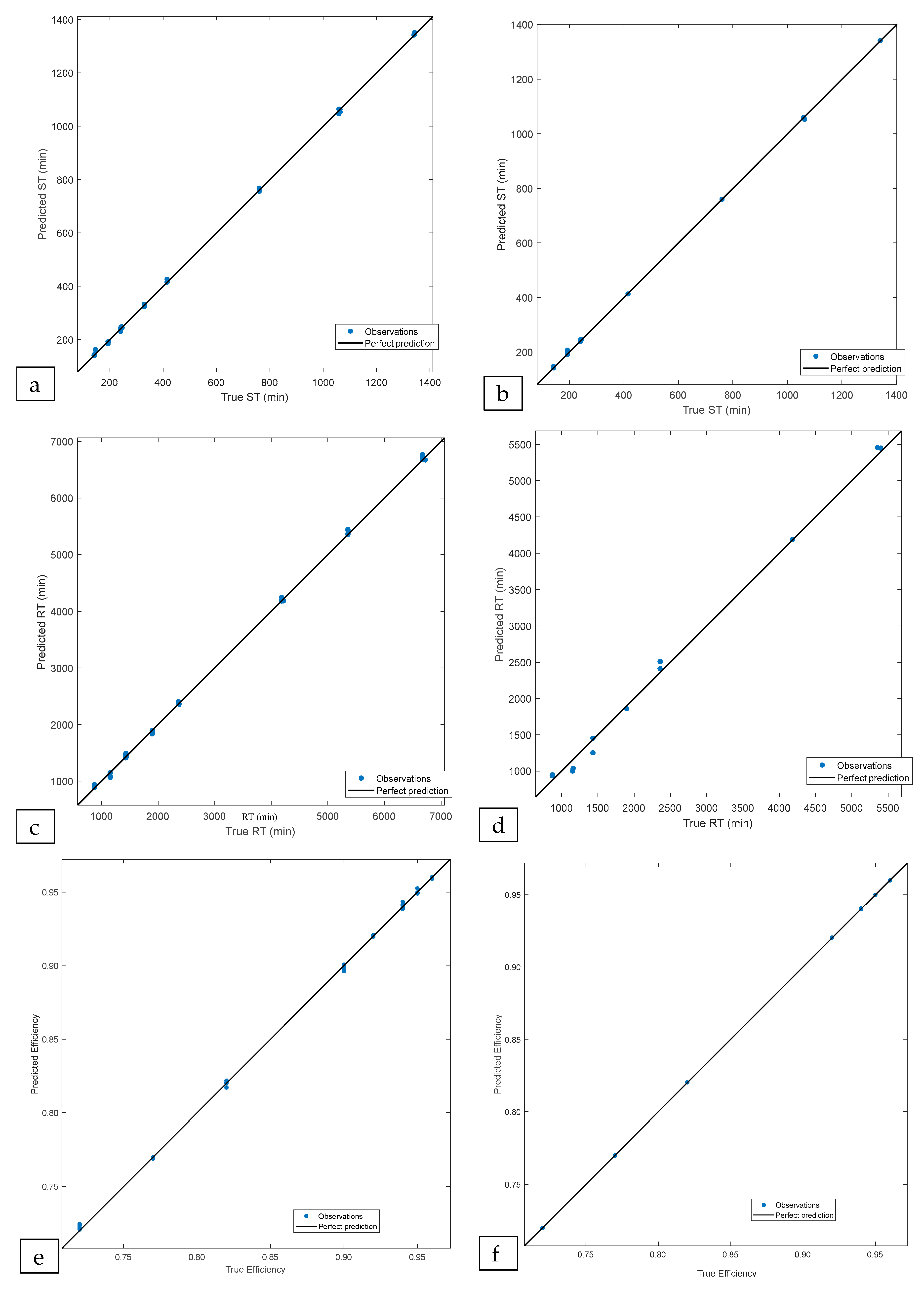
It is of utmost importance to highlight that the selected ML algorithms can serve as practical tools for digitalisation purposes. The true and predicted values of the three responses (ST, RT, and efficiency) can be accurately captured using these techniques, not only during the validation stage but also in the testing stage. Figure 7 presents the comparison between the true and predicted values. Overall, the Gaussian Process Regression and Neural Network models are capable of achieving an almost perfect fit, as illustrated by the 45° reference line (black line) in the plots. The proposed ML models showed good agreement in both the validation and testing stages, indicating that overfitting was not present. In this case, the dataset of 54 points proved suitable for calibrating the models, as the results obtained with Aspen software followed a trend that the ML models could effectively capture.

3.4. Comparison with Results from the Literature

The results generated by simulating a compact bed column, utilising cedar sawdust waste as an adsorbent on an industrial scale, were evaluated against values reported in previous studies. It is important to note that these comparisons are relative, as the research consulted was conducted under different operating conditions (e.g., flow rate, height, adsorption capacity, and regeneration) and with varying types of adsorbent.
Analysis of the data obtained indicates that cedar sawdust, used as a filling medium in an industrial-scale bed, performs efficiently in removing methylene blue and safranin from aqueous media. Table 6 summarises the values from the literature together with those achieved in this work.
In comparison with previous studies, it is evident that the Langmuir, Freundlich, and Langmuir–Freundlich isotherm models, when combined with the LDF kinetic model, provide values that are more representative of the actual behaviour of the process. This is attributed to the use of parameters at an industrial scale, where key variables such as inlet flow rate, initial concentration, and bed height were selected based on operating conditions reported in the literature. Within this framework, the differences between the findings of this study and those reported elsewhere can be explained by the more demanding operating conditions applied here, which justifies the apparent discrepancies, as the performance of the adsorbent is strongly influenced by the operating system. Despite this limitation, cedar sawdust offers several strategic advantages, including its low cost, abundance, ease of preparation, and regenerability, which enable its reuse for up to three cycles. These characteristics render it a competitive and sustainable alternative for large-scale applications, where balancing efficiency, economic feasibility, and environmental sustainability is essential.

4. Conclusions

This research demonstrated the potential of cedar sawdust as a bioadsorbent in industrial-scale adsorption columns for the competitive removal of methylene blue and safranin in aqueous solutions. The simulations provided key quantitative data that contribute to the advancement of industrial adsorption processes, showing that a larger adsorption bed prolongs rupture and saturation times, albeit with a slight decrease in efficiency. At the same time, a higher inlet flow rate increases efficiency but shortens these times. These results constitute a technical reference for optimising the design and operation of industrial effluent treatment systems.
This study demonstrates that machine learning algorithms can model RT and ST effectively and efficiently, achieving R2 values over 0.996 during both the validation and testing phases. This result is significant, as it indicates that the analysed process can be digitalised, thereby facilitating the deployment of digital twin models for these operations in water treatment plants.
The integration of Aspen Adsorption with machine learning techniques and the development of digital twins provide engineers with a powerful tool for the design, control, and optimisation of adsorption systems. Aspen software enables the simulation of adsorption columns under various conditions, while machine learning techniques help accelerate scenario analysis by adjusting sensitive parameters to improve the prediction of equipment behaviour. When combined with digital twins, this approach enables continuous monitoring, preventive maintenance, and well-informed decision-making that can significantly impact the performance of the system under study.
Future work will include an economic assessment and a techno-economic resilience analysis to evaluate the feasibility and sustainability of the optimal column configuration. In addition, the implementation of digital twin models is an area that has not yet been addressed in the current literature.

Author Contributions

Conceptualization, C.T.-T. and Á.V.-O.; methodology, C.T.-T., Á.V.-O. and M.H.-P.; software, C.T.-T., O.E.C.-H. and M.P.-S.; formal analysis, C.T.-T., Á.V.-O. and M.H.-P.; writing—original draft preparation, C.T.-T., Á.V.-O. and M.H.-P.; writing—review and editing, O.E.C.-H. and M.P.-S. All authors have read and agreed to the published version of the manuscript.

Funding

This research received no external funding.

Data Availability Statement

The data supporting the results of this study are available upon request from the corresponding author.

Acknowledgments

The authors thank the Universidad de Cartagena for providing equipment and reagents to conduct this research.

Conflicts of Interest

The authors declare no conflicts of interest.

Abbreviations

The following abbreviations are used in this manuscript:
a Output vector;
b Langmuir constant (L/mg), which indicates the affinity of the adsorbate for the adsorbent surface/bias vector;
C e Equilibrium concentration of the contaminant in solution (mg/L);
C f Contaminant concentration at the column outlet (mg/L);
C 0 Inlet contaminant concentration (mg/L);
1     ( C f / C 0 )Indicates the adsorption process efficiency (−, %);
f Latent variable;
H Matrix of basis functions;
K Affinity or adsorption energy constant [(L/mg)n];
k f Freundlich constant, which indicates the adsorption capacity ((mg/g) (mL/g)n);
i Location within the adsorption bed where the equation is being evaluated (-);
I Identity matrix (-);
I W Input weight matrix (-);
L W Layer weight matrix (-);
N Total number of observations (-);
n Surface heterogeneity factor (-);
1 / n Reflects the influence of the initial concentration on the adsorption capacity;
M T C s k Mass transfer coefficient (1/s);
P i Predicted value of a response (min, %);
p Input vector;
q e Adsorption capacity of the contaminant at equilibrium (mg/g);
q m a x Maximum loading capacity of the adsorbent (mg/g);
T i True value of a response (min,%);
W Weight matrix (-);
w k Concentration   of   the   adsorbed   contaminant   on   the   solid   phase   for   component   k (mg/g);
w k * Amount that would be adsorbed if the system were in instantaneous equilibrium with the fluid phase (mg/g);
X Analysed predictor;
y Response variable (min, %);
Δ z Distance between two nodes in the discretised bed (m);
Γ i 1 Previous node in the direction of flow (-);
Γ i Contaminant   concentration   in   the   fluid   phase   at   position   i (mol/m3).
β Coefficient computed from the dataset (-);
σ 2 Error variance

References

  1. Dwivedi, Y.D.; Manoj Kumar, P.; Gupta, A.; Ahalya, N.; Rana, D.; Sharma, M.; Surakasi, R. Experimental Study on the Treatment of Urban Garment Industry Wastewater to Mitigate Groundwater Contamination Using a Solar Evaporative Still. Urban Clim. 2023, 49, 101435. [Google Scholar] [CrossRef]
  2. Ravindiran, G.; Jeyaraju, R.M.; Nandipati, G.; Seerangagounder, S.; Al-Zaqri, N.; Boshaala, A.; Hayder, G. Prevention of Groundwater Contamination from the Pollutants Released from Dyeing Industries Using Biochar Produced from Palm Shell. Urban Clim. 2023, 49, 101515. [Google Scholar] [CrossRef]
  3. Negash, A.; Tibebe, D.; Mulugeta, M.; Kassa, Y. A Study of Basic and Reactive Dyes Removal from Synthetic and Industrial Wastewater by Electrocoagulation Process. S. Afr. J. Chem. Eng. 2023, 46, 122–131. [Google Scholar] [CrossRef]
  4. Al-Tohamy, R.; Ali, S.S.; Li, F.; Okasha, K.M.; Mahmoud, Y.A.G.; Elsamahy, T.; Jiao, H.; Fu, Y.; Sun, J. A Critical Review on the Treatment of Dye-Containing Wastewater: Ecotoxicological and Health Concerns of Textile Dyes and Possible Remediation Approaches for Environmental Safety. Ecotoxicol. Environ. Saf. 2022, 231, 113160. [Google Scholar] [CrossRef] [PubMed]
  5. Badawi, A.K.; Salama, R.S.; Mostafa, M.M.M. Natural-Based Coagulants/Flocculants as Sustainable Market-Valued Products for Industrial Wastewater Treatment: A Review of Recent Developments. RSC Adv. 2023, 13, 19335–19355. [Google Scholar] [CrossRef]
  6. Boinpally, S.; Kolla, A.; Kainthola, J.; Kodali, R.; Vemuri, J. A State-of-the-Art Review of the Electrocoagulation Technology for Wastewater Treatment. Water Cycle 2023, 4, 26–36. [Google Scholar] [CrossRef]
  7. Ravindiran, G.; Sundaram, H.; Rajendran, E.M.; Ramasamy, S.; Nabil, A.Z.; Ahmed, B. Removal of Azo Dyes from Synthetic Wastewater Using Biochar Derived from Sewage Sludge to Prevent Groundwater Contamination. Urban Clim. 2023, 49, 101502. [Google Scholar] [CrossRef]
  8. Sukmana, H.; Bellahsen, N.; Pantoja, F.; Hodur, C. Adsorption and Coagulation in Wastewater Treatment—Review. Prog. Agric. Eng. Sci. 2021, 17, 49–68. [Google Scholar] [CrossRef]
  9. Taiwo, A.F.; Chinyere, N.J. Sorption Characteristics for Multiple Adsorption of Heavy Metal Ions Using Activated Carbon from Nigerian Bamboo. J. Mater. Sci. Chem. Eng. 2016, 4, 39–48. [Google Scholar] [CrossRef]
  10. Homagai, P.L.; Poudel, R.; Poudel, S.; Bhattarai, A. Adsorption and Removal of Crystal Violet Dye from Aqueous Solution by Modified Rice Husk. Heliyon 2022, 8, e09261. [Google Scholar] [CrossRef]
  11. Salah Omer, A.; El Naeem, G.A.; Abd-Elhamid, A.I.; Farahat, O.O.M.; El-Bardan, A.A.; Soliman, H.M.A.; Nayl, A.A. Adsorption of Crystal Violet and Methylene Blue Dyes Using a Cellulose-Based Adsorbent from Sugercane Bagasse: Characterization, Kinetic and Isotherm Studies. J. Mater. Res. Technol. 2022, 19, 3241–3254. [Google Scholar] [CrossRef]
  12. Akter, M.; Rahman, F.B.A.; Abedin, M.Z.; Kabir, S.M.F. Adsorption Characteristics of Banana Peel in the Removal of Dyes from Textile Effluent. Textiles 2021, 1, 361–375. [Google Scholar] [CrossRef]
  13. Li, B.; Ma, R.; Jiang, J.; Guo, L.; Li, K. Deployment of interpretable machine learning in a water treatment device—feasibility exploration of performance enhancement. J. Water Process Eng. 2024, 58, 104781. [Google Scholar] [CrossRef]
  14. Rodríguez-Alonso, C.; Pena-Regueiro, I.; García, Ó. Digital Twin Platform for Water Treatment Plants Using Microservices Architecture. Sensors 2024, 24, 1568. [Google Scholar] [CrossRef] [PubMed]
  15. Wang, A.J.; Li, H.; He, Z.; Tao, Y.; Wang, H.; Yang, M.; Savic, D.; Daigger, G.T.; Ren, N. Digital Twins for Wastewater Treatment: A Technical Review. Engineering 2024, 36, 21–35. [Google Scholar] [CrossRef]
  16. Pylianidis, C.; Snow, V.; Overweg, H.; Osinga, S.; Kean, J.; Athanasiadis, I.N. Simulation-assisted machine learning for operational digital twins. Environ. Model. Softw. 2022, 148, 105274. [Google Scholar] [CrossRef]
  17. Nieva, A.D.; Garcia, R.C.; Ped, R.M. Simulated Biosorption of Cr6+ Using Peels of Litchi chinensis sonn by Aspen Adsorption® V8.4. Int. J. Environ. Sci. Dev. 2019, 10, 331–337. [Google Scholar] [CrossRef]
  18. Durán-García, M.E.; Ruiz-Navas, R.A. Simulator of thermodynamic properties in the conversion of forest biomass of pine sawdust. Maderas Cienc. Tecnol. 2020, 22, 347–364. [Google Scholar] [CrossRef]
  19. Soriano, A.N.; Orfiana, O.N.; Pangon, M.B.J.; Nieva, A.D.; Adornado, A.P. Simulated Biosorption of Cd(II) and Cu(II) in Single and Binary Metal Systems by Water Hyacinth (Eichhornia crassipes) Using Aspen Adsorption®. ASEAN J. Chem. Eng. 2016, 16, 21–43. [Google Scholar] [CrossRef]
  20. Hameed, A.; Hameed, B.H.; Almomani, F.A.; Usman, M.; Ba-Abbad, M.M.; Khraisheh, M. Dynamic simulation of lead(II) metal adsorption from water on activated carbons in a packed-bed column. Biomass Convers. Biorefinery 2024, 14, 8283–8292. [Google Scholar] [CrossRef]
  21. Nikam, S.; Mandal, D.; Dabhade, P. LDF Based Parametric Optimization to Model Fluidized Bed Adsorption of Trichloroethylene on Activated Carbon Particles. Particuology 2022, 65, 72–92. [Google Scholar] [CrossRef]
  22. Ragadhita, R.; Bayu, A.; Nandiyanto, D. Curcumin Adsorption on Zinc Imidazole Framework-8 Particles: Isotherm Adsorption Using Langmuir, Freundlich, Temkin, And Dubinin-Radushkevich Models. J. Eng. Sci. Technol. 2022, 17, 1078–1089. [Google Scholar]
  23. Ezzati, R. Derivation of Pseudo-First-Order, Pseudo-Second-Order and Modified Pseudo-First-Order Rate Equations from Langmuir and Freundlich Isotherms for Adsorption. Chem. Eng. J. 2020, 392, 123705. [Google Scholar] [CrossRef]
  24. Stromer, B.S.; Woodbury, B.; Williams, C.F. Tylosin Sorption to Diatomaceous Earth Described by Langmuir Isotherm and Freundlich Isotherm Models. Chemosphere 2018, 193, 912–920. [Google Scholar] [CrossRef]
  25. Fouad, M.R. Physical Characteristics and Freundlich Model of Adsorption and Desorption Isotherm for Fipronil in Six Types of Egyptian Soil. Curr. Chem. Lett. 2023, 12, 207–216. [Google Scholar] [CrossRef]
  26. Jeppu, G.P.; Clement, T.P. A Modified Langmuir-Freundlich Isotherm Model for Simulating PH-Dependent Adsorption Effects. J. Contam. Hydrol. 2012, 129–130, 46–53. [Google Scholar] [CrossRef]
  27. Amrutha; Jeppu, G.; Girish, C.R.; Prabhu, B.; Mayer, K. Multi-Component Adsorption Isotherms: Review and Modeling Studies. Environ. Process. 2023, 10, 1–52. [Google Scholar] [CrossRef]
  28. De Araujo, C.M.B.; Ghislandi, M.G.; Rios, A.G.; da Costa, G.R.B.; do Nascimento, B.F.; Ferreira, A.F.P.; da Motta Sobrinho, M.A.; Rodrigues, A.E. Wastewater Treatment Using Recyclable Agar-Graphene Oxide Biocomposite Hydrogel in Batch and Fixed-Bed Adsorption Column: Bench Experiments and Modeling for the Selective Removal of Organics. Colloids Surf. A Physicochem. Eng. Asp. 2022, 639, 128357. [Google Scholar] [CrossRef]
  29. Dadebo, D.; Atukunda, A.; Ibrahim, M.G.; Nasr, M. Integrating Chemical Coagulation with Fixed-Bed Column Adsorption Using Rice Husk-Derived Biochar for Shipboard Bilgewater Treatment: Scale-up Design and Cost Estimation. Chem. Eng. J. Adv. 2023, 16, 100520. [Google Scholar] [CrossRef]
  30. Agarwal, A.; Upadhyay, U.; Sreedhar, I.; Anitha, K.L. Simulation Studies of Cu(II) Removal from Aqueous Solution Using Olive Stone. Clean. Mater. 2022, 5, 100128. [Google Scholar] [CrossRef]
  31. Villabona-Ortiz, Á.; Tejada-Tovar, C.; González-Delgado, Á. Parametric Evaluation of a Packed Adsorption Column to Remove Cr (VI) Using Langmuir and Freundlich with (LDF) and (QDF). Desalination Water Treat. 2025, 321, 101023. [Google Scholar] [CrossRef]
  32. Singh, V.; Nemalipuri, P.; Vitankar, V.; Das, H.C. Multifluid Computational Fluid Dynamics Simulation for Sawdust Gasification inside an Industrial Scale Fluidized Bed Gasifier. Mater. Today Proc. 2023. [Google Scholar] [CrossRef]
  33. Koua, B.K.; Koffi, P.M.E.; Gbaha, P. Evolution of Shrinkage, Real Density, Porosity, Heat and Mass Transfer Coefficients during Indirect Solar Drying of Cocoa Beans. J. Saudi Soc. Agric. Sci. 2019, 18, 72–82. [Google Scholar] [CrossRef]
  34. Babalola, J.O.; Koiki, B.A.; Eniayewu, Y.; Salimonu, A.; Olowoyo, J.O.; Oninla, V.O.; Alabi, H.A.; Ofomaja, A.E.; Omorogie, M.O. Adsorption Efficacy of Cedrela Odorata Seed Waste for Dyes: Non Linear Fractal Kinetics and Non Linear Equilibrium Studies. J. Environ. Chem. Eng. 2016, 4, 3527–3536. [Google Scholar] [CrossRef]
  35. Rasmussen, C.E.; Williams, C.K.I. Gaussian Processes for Machine Learning; MIT Press: Cambridge, MA, USA, 2006. [Google Scholar] [CrossRef]
  36. Demuth, H.; Beale, M.; Hagan, M. Neural Network Toolbox; For Use with MATLAB; MathWorks Inc.: Carlsbad, CA, USA, 2004; Volume 4. [Google Scholar]
  37. Zhang, Y.P.; Adi, V.S.K.; Huang, H.L.; Lin, H.P.; Huang, Z.H. Adsorption of Metal Ions with Biochars Derived from Biomass Wastes in a Fixed Column: Adsorption Isotherm and Process Simulation. J. Ind. Eng. Chem. 2019, 76, 240–244. [Google Scholar] [CrossRef]
  38. Rial, A.; Pimentel, C.H.; Gómez-Díaz, D.; Freire, M.S.; González-Álvarez, J. Evaluation of Almond Shell Activated Carbon for Dye (Methylene Blue and Malachite Green) Removal by Experimental and Simulation Studies. Materials 2024, 17, 6077. [Google Scholar] [CrossRef]
  39. Hoseini Dastgerdi, Z.; Meshkat, S.S.; Jalili, H. Investigation of an Adsorptive Indigo Carmine Dye Removal via Packed Bed Column: Experiments and Computational Fluid Dynamics Simulation. AUT J. Mech. Eng. 2020, 4, 315–330. [Google Scholar] [CrossRef]
  40. Baharlouei, A.; Jalilnejad, E.; Sirousazar, M. Fixed-bed column performance of methylene blue biosorption by Luffa cylindrica: Statistical and mathematical modeling. Chem. Eng. Commun. 2018, 205, 1537–1554. [Google Scholar] [CrossRef]
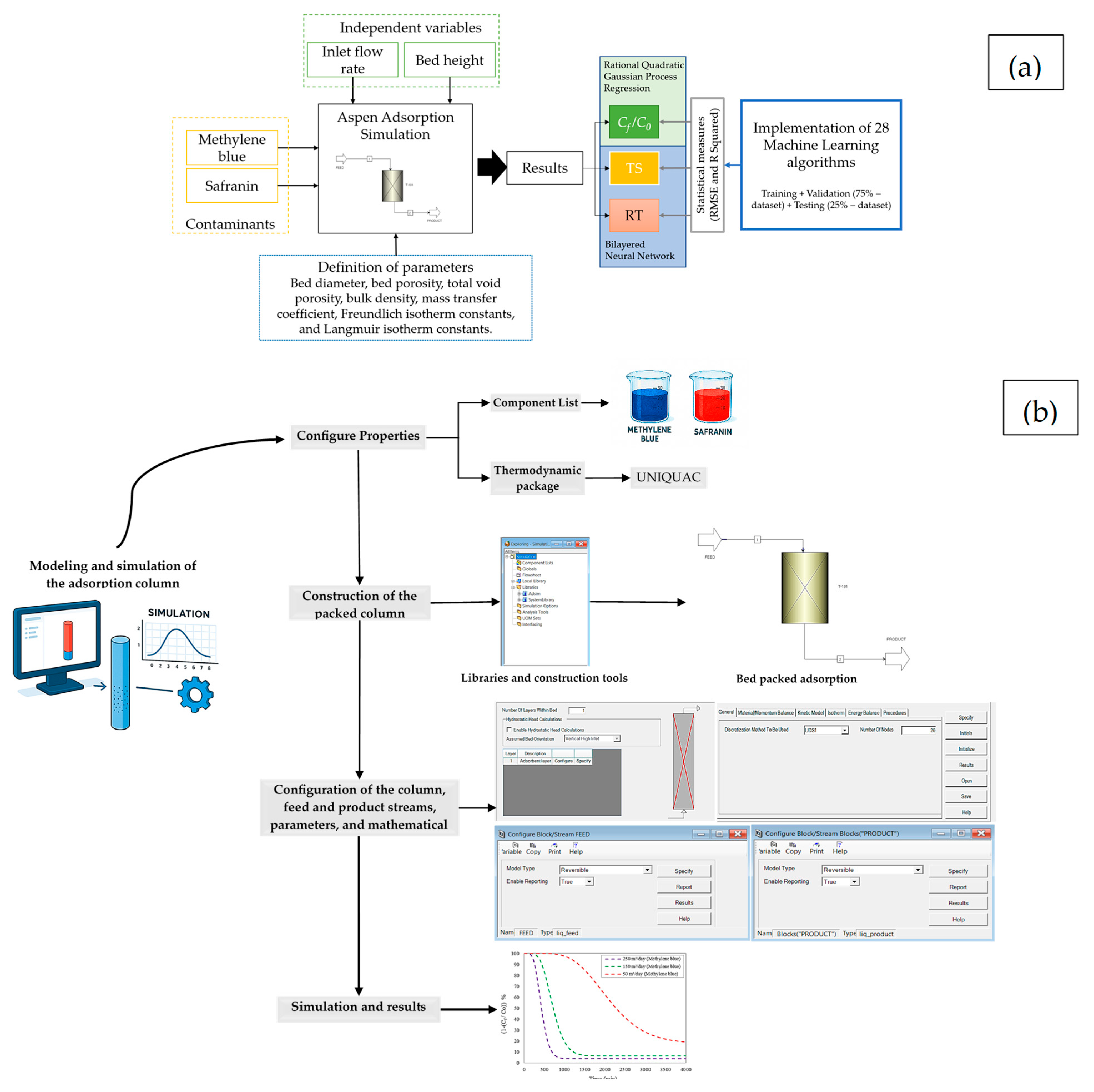
Figure 1. Methodology employed in this study: (a) general overview; (b) Aspen Adsorption software.
Processes 13 02907 g001
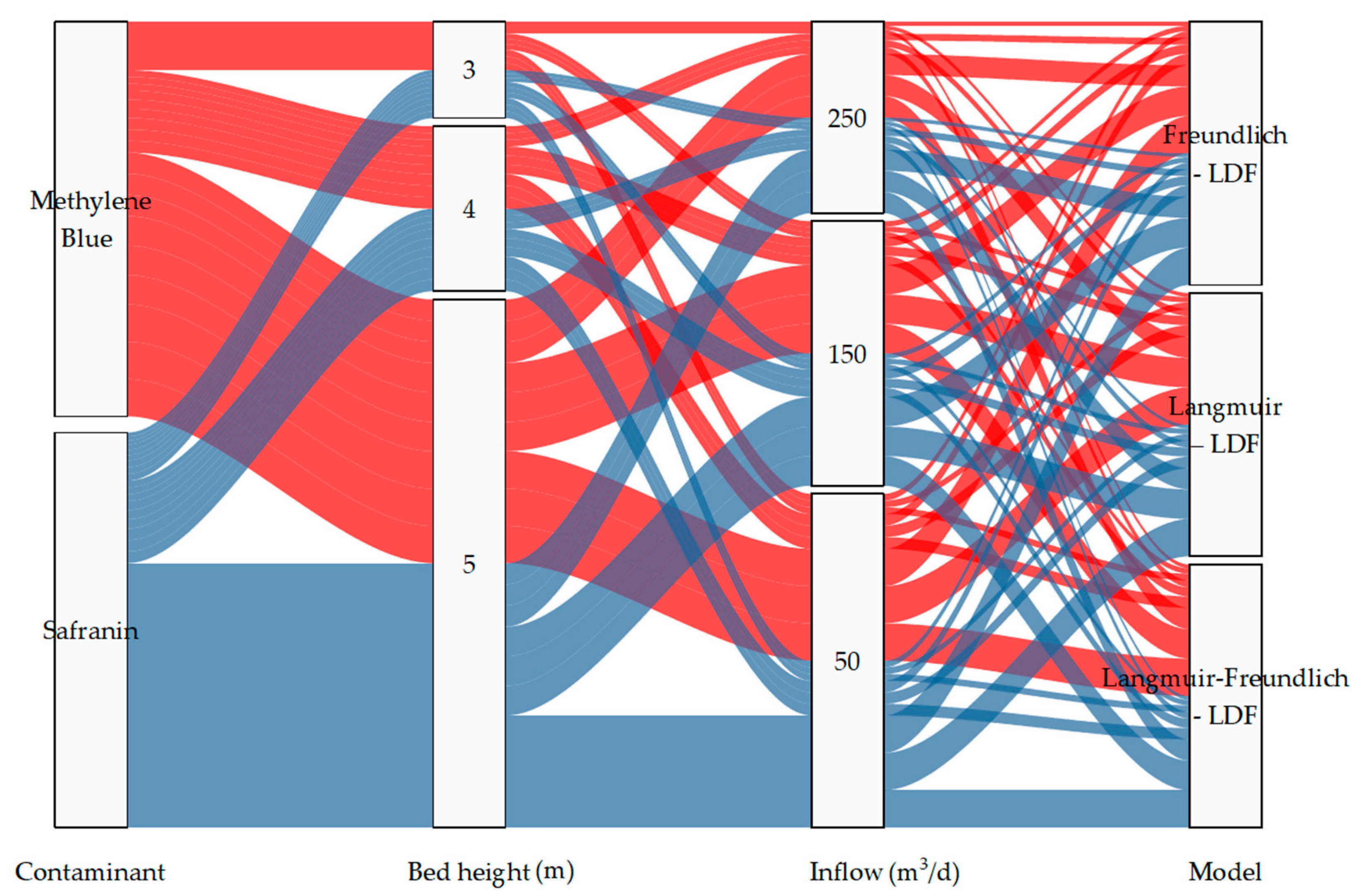
Figure 2. Relationships between predictors.
Processes 13 02907 g002
Figure 3. Structure of a bilayered neural network.
Processes 13 02907 g003
Figure 4. Removal of contaminant profiles at different simulated inlet flows using the Freundlich–LDF model (a,b), the Langmuir–LDF model (c,d), and the Langmuir–Freundlich–LDF model (e,f). C f represents the contaminant concentration at the column outlet, C 0 is the inlet contaminant concentration, and the ratio (1 − C f / C 0 ) indicates the adsorption process efficiency.
Processes 13 02907 g004
Figure 5. Removal of contaminant profiles at different simulated bed height using the Freundlich–LDF model (a,b), the Langmuir–LDF model (c,d), and the Langmuir–Freundlich–LDF model (e,f). C f represents the contaminant concentration at the column outlet, C 0 is the contaminant concentration at the column inlet, and the ratio (1 − C f / C 0 ) indicates the efficiency of the adsorption process.
Processes 13 02907 g005
Figure 6. Statistical measures of the employed 28 MLAs for validation and test phases: (a) for ST, R-squared; (b) for ST, RMSE; (c) for RT, R-squared; (d) for RT, RMSE; (e) for 1 C f / C 0 , R-squared; and (f) for 1 C f / C 0 , RMSE.
Processes 13 02907 g006
Figure 7. Comparison between true and predicted values: (a) ST in the validation stage; (b) ST in the testing stage; (c) RT in the validation stage; (d) RT in the testing stage; (e) efficiency in the validation stage; and (f) efficiency in the testing stage.
Processes 13 02907 g007
Table 2. Range of parameter values considered in the parametric study for dye adsorption.
Independent VariableUnitRangeReference
Inlet flow ratem3/day50, 150, 250[28]
Bed heightm3, 4, 5[29]
Table 3. Parameters used for the simulation of the adsorption column.
ParameterUnitValueReference
Bed diameterm1[30]
Bed porositym3 void/m3 bed0.667[31]
Total void porositym3 void/m3 bed0.4[32]
Bulk densitykg/m31400[32]
Mass transfer coefficient1/s1.37 × 10−4[33]
Freundlich isotherm constants
k f ((mg/g) (mg/L)n)0.205[34]
1 / n 0.058[34]
Langmuir isotherm constants
b L/mg0.958[34]
q m a x mg/g0.262[34]
Langmuir–Freundlich isotherm constants
KLangmuirL/mg0.958[34]
KFreundlich((mg/g) (mg/L)n)0.205[34]
Table 4. ML algorithms used in this research.
Model TypePresent
TreeFine (TF), Medium (TM), and Coarse (TC).
Linear regressionLinear (LRL), Interactions Linear (LRI), and Robust Linear (LRR).
Stepwise Linear RegressionStepwise Linear (SLR).
Support Vector Machine (SVM)Linear (SVML), Quadratic (SVMQ), Cubic (SVMC), Fine Gaussian (SVMF), Medium Coarse (SVMM), and Coarse Gaussian (SVMG).
Efficient LinearEfficient Linear Least Squares (ELE) and Efficient Linear SVM (EEL).
EnsembleBoosted (EBO) and Bagged (EBA) Trees.
Gaussian Process RegressionSquared Exponential (GPRS), Matern 5/2 (GPRM), Exponential (GPRE), and Rational Quadratic (GPRR).
Neural NetworkNarrow (NNN), Medium (NNM), Wide (NNW), Bilayered (NNB), and Trilayered (NNT).
KernelSVM (KSVM) and Least Squares Regression (KLSR).
Table 5. Selected ML algorithms for the responses of Aspen Adsorption.
ResponseSelected ModelR SquaredRMSETraining Time (s)
ValidationTestValidationTest
ST (min)NNB0.9990.9995.5425.2001.81
RT (min)NNB0.9990.99639.61597.6302.89
1 C f / C 0 (%)GPRR0.9990.9990.00160.00033.64
Table 6. Comparative performance of different adsorbents for contaminant removal in packed-bed columns.
ParameterMethylene Blue/
Malachite Green
Indigo CarmineMethylene BlueMethylene Blue/
Safranin
AdsorbentAlmond ShellGrapheneNaOH-modified Luffa cylindricaCedar sawdust
Initial concentration (mg/L)20010392000
Inlet flow rate (m3/day)1.44 × 10−51.44 × 10−21.44 × 10−3250
Bed height (m)0.0240.280.23
Rupture time (min)2620/350087100142/142
Saturation time (min)2690/4000--870/872
Capacity Adsorption (mg/g)341/36434946.60.262; 0.205
Regenerative capacity---3
Reference[38][39][40]This research
Disclaimer/Publisher’s Note: The statements, opinions and data contained in all publications are solely those of the individual author(s) and contributor(s) and not of MDPI and/or the editor(s). MDPI and/or the editor(s) disclaim responsibility for any injury to people or property resulting from any ideas, methods, instructions or products referred to in the content.