Article

A Robust Planning Method for Multi-Village Coupled Rural Micro-Energy Grid Based on Information Gap Decision Theory

1
Economic and Technology Research Institute, State Grid Hebei Electric Power Co., Ltd., Shijiazhuang 050021, China
2
College of Mechanical and Electrical Engineering, Hebei Agricultural University, Baoding 071001, China
3
Baoding Key Laboratory of Precision Environmental Control and Clean Energy Supply for Facility Agriculture, Baoding 071001, China
*
Author to whom correspondence should be addressed.
Processes 2025, 13(9), 2881; https://doi.org/10.3390/pr13092881
Submission received: 8 August 2025 / Revised: 30 August 2025 / Accepted: 6 September 2025 / Published: 9 September 2025
(This article belongs to the Section Energy Systems)

Abstract

The application of rural micro-energy grids is critical for improving the energy economy and supply quality in rural areas, yet existing planning methods suffer from two key limitations: (1) they focus on single-village scenarios, failing to exploit multi-village resource integration potential; and (2) they rarely address operational uncertainties, which pose risks to the feasibility of planning schemes. To fill these gaps, this study proposes a robust planning method for multi-village coupled rural micro-energy grids (MV-RMEGs). Based on the multi-energy coupling model within the MV-RMEG, a collaborative/autonomous operation framework is developed, which balances energy coupling efficiency and supply reliability. By integrating the information gap decision theory into the established deterministic model, multiple uncertainties in MV-RMEG can be handled without relying on probability statistics. Simulation results from a rural area in North China verify the method’s superiority: compared with single-village planning schemes, the proposed method reduces the power purchasing cost by 99.61%; in off-grid scenarios, it maintains a critical load shedding rate of 3.96%, which is 27.27% lower than the deterministic method. Moreover, the uncertainty handling process leads to a 10.25% reduction in the operating cost of the proposed method when dealing with DG output and load fluctuations.

1. Introduction

Traditional rural production and lifestyles contribute significantly to both carbon dioxide emissions and environmental pollution. Against the backdrop of energy structure adjustment and carbon emission reduction, rural areas are actively pursuing the development of modern energy systems, moving towards cleaner, more efficient, and more economical energy supply and consumption structures [1]. Taking China as an example, in 2021, the government issued the “Guiding Opinions on Promoting the Transformation and Development of Rural Energy to Support Rural Revitalization”, emphasizing that rural energy development must adhere to the fundamental principles of clean and low-carbon, ecological and livable, local adaptation, nearby utilization, and economic and reliable, in order to benefit the people and public and accelerate the formation of a green and diversified rural energy system [2].
Rural areas possess abundant wind, solar, and biomass resources. In recent years, the installed capacity of renewable energy has increased rapidly. During peak generation periods, reverse power flow occurs in some areas, compromising grid stability [3,4]. On the demand side, the large-scale emergence of new loads, such as facility agriculture and electric vehicles (EVs), has imposed new requirements on energy supply. Under these new circumstances, rural micro-energy grids (RMEGs), serving as a rural energy system that enables the efficient complementary utilization of electricity, heating, cooling, and other energy forms, have gained significant attention for their role in renewable energy integration and multi-energy coupling [5,6].
Scholars have previously demonstrated the advantages of RMEGs in coupled multi-energy utilization. Ref. [7] constructed an energy comprehensive heating model with solar collectors as the main body and air-source heat pump (ASHP) heating systems as supplements to address the issue of renewable energy consumption. The model takes into account the thermodynamic coupling relationship of each component. Refs. [8,9] refined the biomass–solid waste supply chain model within the RMEG, effectively reducing energy costs during peak load periods. Refs. [10,11,12] developed a two-stage optimization scheduling model for multi-energy coupling in the RMEG. Building upon economic and ecological benefits, this model further ensures the robustness of the scheduling scheme against adverse operating conditions. The research above confirms that RMEGs are critical for the economic and stable operation of rural integrated energy.
Preliminary planning is crucial for the operational performance of RMEGs [13]. Among planning aspects, the sizing of key equipment constitutes the core content of RMEG planning [14,15]. Table 1 compares the state of the art of RMEG planning studies to analyze the research gaps.
As shown in Table 1, most existing literature has optimized the capacity of energy equipment based on typical daily data from the target area. By summarizing, there are mainly two research gaps:
  • All of the studies predominantly focus on meeting the energy demands of a single village. Although Refs. [16,20] optimize many energy equipment, these devices still belong to an RMEG composed of a single village. That is, both the energy production and consumption of each equipment are confined to a single and definite entity. In reality, significant differences exist in industrial structures and energy supply–demand relationships between neighboring villages, accompanied by strong complementary effects. Therefore, further research is warranted to leverage the respective resource characteristics of each village and establish a multi-village coupled RMEG (MV-RMEG). The challenge of developing a framework to integrate the energy facilities of multiple villages into a single system, while ensuring their operation during off-grid periods, needs to be addressed.
  • Most studies adopt deterministic optimization strategies, ignoring the uncertainties during the operation of RMEG. Actually, the distributed generation (DG) output in RMEGs exhibits significant randomness. Neglecting the uncertainty issues degrades the optimality of the planning scheme [25]. The simulation results based on historical data and predicting values clearly cannot take into account the impact of these fluctuations. Ref. [23] considers meteorological data fluctuations in numerical simulations, but the proposed model still belongs to deterministic optimization. Although Refs. [19,22] handle the uncertainties leveraging the robust optimization, the feasibility of the planning scheme is poor due to the overly conservative nature of the method. Therefore, an effective approach is required to properly handle the uncertainties in the MV-RMEG planning process.
In summary, in the current research on RMEGs, the complementarity and independence among multiple villages have not been considered. Moreover, in the planning process, the impact brought by the DG randomness needs to be fully considered to enhance the applicability of the planning scheme. To address the above issues, this study proposes a robust planning method for an MV-RMEG, expanding the research scope from a single village to the collaboration of multiple villages. The contributions of this paper are as follows:
  • A planning method for the MV-RMEG under the collaborative/autonomous operation framework is proposed. The planning scheme can achieve interconnection and mutual assistance among multiple villages during regular operation. Simultaneously, it ensures a reliable energy supply to critical loads during off-grid periods.
  • The stochastic nature of DG output and load within the MV-RMEG is effectively addressed by applying the information gap decision theory (IGDT). The proposed method enables the artificial control of the robustness level of optimization results without relying on such prior information. This endows the planning scheme with enhanced robustness against operational uncertainties.
The rest of the article is organized as follows: in Section 2, the models of components in MV-RMEG are established. In Section 3, the collaborative/autonomous operation framework for MV-RMEG is developed. Based on this, we formulate the planning method under deterministic conditions. In Section 4, the IGDT-based uncertainty handling method is proposed. Section 5 analyzes the numerical simulation results. Finally, the conclusions are summarized in Section 6.

2. Modeling of MV-RMEG Components

This study constructs an MV-RMEG to enhance renewable energy consumption and new load carrying. The internal structure of the proposed MV-RMEG is depicted in Figure 1. The abundant photovoltaic (PV) and wind resources prevalent in rural areas are fully utilized to meet the local electrical demand. Rural loads encompass electricity, heating, and cooling needs, satisfying the energy requirements for production and daily life. Utilizing biomass resources, such as livestock manure generated from animal husbandry, represents an essential pathway for green energy development in rural areas. In this study, biomass resources undergo anaerobic digestion to produce biogas. This biogas is fed into and combined with a heat and power (CHP) system for electricity and heat generation. The high-temperature exhaust gases from the CHP are further utilized via a waste heat recovery boiler. Absorption chillers (ACs) and ASHPs enable efficient energy conversion, providing supplementary cooling and heating energy. EVs interact bidirectionally with the grid through vehicle-to-grid (V2G) charging piles. They function as flexible loads that participate in the optimal dispatch of the power grid.

2.1. DG Modeling

The output of distributed wind turbines (WTs) mainly depends on the wind speed at the turbine hub. The measured wind speed is first converted according to the difference in height between the wind measurement point and the hub height as follows:
v ( t ) = v r e f ( t ) H H r e f α
where v(t) and vref(t) represent the wind speed at the hub and the measurement point, respectively. H and Href represent the hub and measurement point heights, respectively. α is the coefficient of surface roughness, which is set to 0.22 in this study.
In actual operation, the maximum output value of a WT at each moment can be expressed in the form of a segmented linear function as follows:
P ¯ w ( t ) = 0 v ( t ) v i n P w , r a t e v ( t ) v i n v r v i n v i n v ( t ) v r P w , r a t e v r v ( t ) v out 0 v ( t ) v out
where P ¯ pv ( t ) and Pw,rate represent the upper limit of a single WT’s output at time t and its rated power, respectively. vin and vout represent the WT’s cut-in and cut-out wind speeds, respectively. vr is the rated wind speed.
The PV output depends on irradiance, temperature, and the area of the PV panel, and can be expressed as
P ¯ pv ( t ) = f pv P pv , rate A ( t ) A s 1 + α pv T 0 ( t ) T stc
where P ¯ pv ( t ) and Ppv,rate represent the upper limit of the output power at time t and the rated power of a single PV panel, respectively. fpv is the PV energy conversion efficiency. A(t) and As represent the irradiance and rated irradiance, respectively. αpv is the power temperature coefficient. T0(t) and Tstc represent the actual temperature and the temperature of the PV module under standard test conditions, respectively.

2.2. CHP Modeling

Biogas represents a distinctive biomass resource characteristic of rural areas. Against the current trend towards intensive breeding in rural regions, large-scale livestock farms generate substantial quantities of livestock manure. Utilizing these manure resources for constant-temperature anaerobic digestion to produce biogas partially fulfills the fuel requirements for electricity and heat generation and contributes to reducing environmental pollution. Firstly, the daily biogas yield is calculated based on the livestock species and farm scale as follows:
V b mat = B b M b
V met = b θ b bio V b mat
where V b mat is the daily manure production of the bth livestock or poultry, Bb is the breeding scale, Mb represents the daily manure production per single animal, Vmet represents the total daily biogas production, and θ b bio represents the biogas production rate of the manure of the bth livestock or poultry.
The produced biogas can be used to generate electricity via micro gas turbines or produce heating power through biogas boilers. A waste heat recovery boiler can collect the high-temperature exhaust gases from the gas turbines to supplement the heat output. Referring to Ref. [26], the model for CHP can be mathematically represented as:
Q mt ( t ) = P mt ( t ) 1 η mt , e η hl η mt , e
V mt ( t ) = P mt ( t ) θ cal η mt , e
Q bb ( t ) = V bb ( t ) θ cal η bb
Q whr ( t ) = Q mt ( t ) η whr , r η whr , h
0 t V mt ( t ) + V bb ( t ) V met
where Qmt(t) and Pmt(t) represent the heating power and electrical power output by the gas turbine, respectively. ηmt,e and ηhl represent the power generation efficiency and heat loss coefficient of the gas turbine, respectively. Qbb(t) and Qwhr(t) represent the heating power of the biogas boiler and the waste heat recovery boiler, respectively. Vbg(t) and Vbb(t) represent the biogas consumption of the gas turbine and the biogas boiler, respectively. θcal is the calorific value of biogas, and ηbb is the thermal efficiency of the biogas boiler, while ηwhr,r and ηwhr,h represent the heat recovery efficiency and thermal efficiency of the waste heat boiler, respectively.

2.3. ASHP Modeling

ASHPs are characterized by a high coefficient of performance (COP). They are an energy-efficient alternative to traditional electric heating or cooling equipment, achieving effective heating or cooling outcomes with significantly lower energy consumption. Currently, ASHPs have been widely adopted in rural areas. The ASHP model can be mathematically represented as follows [27]:
Q ashp ( t ) = P ashp , h ( t ) C O P ashp ( t )
C ashp ( t ) = P ashp , c ( t ) C O P ashp ( t )
P ashp , h ( t ) + P ashp , c ( t ) = P ashp ( t )
0 P ashp ( t ) P ¯ ashp
where Qashp(t), Cashp(t), Pashp,h(t), and Pashp,c(t) represent the heating and cooling power of the ASHP, as well as the corresponding electric power. P ¯ ashp is the planned capacity of the ASHP. COPashp(t) is the COP of the ASHP, which is a parameter that is related to the ambient temperature at each time slot. The specific values of COPashp can be found in Ref. [28].

2.4. AC Modeling

ACs utilize naturally occurring refrigerants such as water or ammonia to convert thermal energy into cooling output. They are characterized by structural simplicity, operational safety, and installation convenience, which helps alleviate the pressure on power load caused by high refrigeration demand. In this study, the AC serves as an effective complement to ASHP refrigeration. Referring to Ref. [29], its mathematical model can be represented as follows:
C ac ( t ) = Q ac ( t ) C O P ac ( t )
0 Q ac ( t ) Q ¯ ac
where Cac(t) and Qac(t) represent the cooling output and heat power of the AC, respectively. Q ¯ ac indicates the planned capacity of the AC. COPac(t) is the COP of the AC. Similar to ASHP modeling, COPac is also affected by ambient temperature. The specific parameter values can be found in Ref. [30].

2.5. EV Modeling

With rising living standards in rural areas and the strong promotion of policies facilitating EV adoption, the household penetration rate of EVs in rural regions has been increasing annually. Their charging load poses a challenge to the power grid. On the other hand, by leveraging V2G technology, EVs can perform bidirectional power regulation with the grid, providing support for peak shaving. A model of EV travel patterns is first established to characterize the charging load. Based on statistical evidence, EVs’ arrival and departure times follow a normal distribution [31].
f t arr / dep = 1 σ arr / dep 2 π exp t arr / dep μ arr / dep 2 2 σ arr / dep ­ 2
where tarr/dep represents the time an EV arrives at or departs from the charging station. μarr/dep and σarr/dep are the corresponding mean and standard deviation, respectively. The daily driving mileage of an EV follows a log-normal distribution [32].
f d = 1 d σ d 2 π exp ln d μ d 2 2 σ d2
where d is the daily driving mileage of the EV, while μd and σd denote the mean and standard deviation of the daily driving mileage, respectively.
Based on the obtained daily driving mileage, the initial state of charge (SOC) at the charging moment can be expressed as
S ( t arr ) = E ev d θ ev E ev
where θev is the average power consumption per kilometer of the EV, and Eev represents the rated capacity of the EV battery. The power battery of an EV can be regarded as an equivalent electrochemical energy storage device. Therefore, based on the modeling of energy storage devices, the charging process of an EV during grid connection can be described in the following dynamic form [33]:
S lb S i ( t ) 1
u i ( t ) P ¯ dis P i ev ( t ) u i ( t ) P ¯ ch
E i ev ( t + 1 ) = E i ev ( t ) + P i ev ( t ) η ch P i ev 0 E i ev ( t ) + P i ev ( t ) / η dis P i ev 0
i u i ( t ) N pile
P sta ( t ) = i P i ev ( t )
where Si(t) is the SOC of the ith EV at time t. Slb is the lower limit of the SOC. E i ev ( t ) and P i ev ( t ) are the battery energy and the power exchanged with the grid of the ith EV, respectively. P ¯ ch / dis represents the rated charging/discharging power of the EV. ui(t) is a binary variable indicating whether the EV is connected to the grid. ηch/dis represents the charging/discharging efficiency. Npile is the number of charging piles. Psta is the power of the entire charging station.

2.6. Facility Agriculture and Livestock Farming Modeling

Temperature is critical for environmental control in facility agriculture and large-scale livestock farming. Temperature regulation can be achieved by adopting indoor heating, ventilation, and air conditioning (HVAC) equipment. The corresponding load model for greenhouses and livestock facilities can be represented as follows [34]:
T in ( t + 1 ) = T in ( t ) + Q sup ( t ) C sup ( t ) Q loss ( t ) C m d Q loss ( t ) = δ loss S T in ( t ) T out ( t )
where Tin(t) is the indoor temperature at time t. Qsup(t) and Qloss(t) are the heat power provided by the heating equipment and the heat transfer power between indoors and outdoors, respectively. Csup(t) is the supplementary cooling power. Cm is the specific heat capacity of air. d is the indoor air mass. δloss is the heat transfer coefficient. S is the surface area of the heat exchange region between indoors and outdoors.

2.7. Network Modeling

The distribution network model is constructed by using the Distflow equations. The second-order cone constraint is adopted to keep the model convex.
k Λ j + P j k ( t ) i Λ j P i j ( t ) I ˜ i j ( t ) r i j = P j k Λ j + Q j k ( t ) i Λ j Q i j ( t ) I ˜ i j ( t ) x i j = Q j U ˜ j ( t ) = U ˜ i ( t ) 2 P i j ( t ) r i j + Q i j ( t ) x i j + I ˜ i j ( t ) r i j 2 + x i j 2 2 P i j ( t ) 2 Q i j ( t ) I ˜ i j ( t ) U ˜ i ( t ) 2 I ˜ i j ( t ) + U ˜ i ( t )
where Λ j is the set for all starting buses ending in j. Λ j + is the set that contains all ending buses starting from j. Pij and Qij represent the sending-end active and reactive power from bus i to j, respectively. Pj and Qj represent the active and reactive power injected into bus j, respectively. I ˜ ij and U ˜ j represent the squared magnitude of current/voltage after the phase angle relaxation, respectively. Rij and Xij represent the resistance and reactance of branch ij, respectively.
The model of the heating system contains primary and secondary networks. For the primary network, a quantity regulation method is adopted to set the pipeline flow.
j Ψ i + q j ( t ) = k Ψ i q k ( t ) T j out ( t ) j Ψ i + q j ( t ) = k Ψ i T k in ( t ) q k ( t ) H i S ( t ) = c w m i S ( t ) T i g ( t ) T i h ( t ) Q i S ( t ) Δ t = H i S ( t ) T j end ( t ) = T j start ( t ) T 0 ( t ) e λ L j c w q j ( t ) + T 0 ( t )
where Ψ i + and Ψ i represent the sets of pipeline branches that start and end from node i, respectively. qj is the hot water mass flow rate in branch j. T k out is the outlet temperature of hot water in branch j. T j in is the inlet temperature of hot water in branch k. H i S is the total heat exchange. cw is the specific heat capacity of the transmission medium. m i S is the total mass of hot water. T i g and T i h represent the supply water temperature and return water temperature, respectively. Q i S is the heat power. T j end is the hot water temperature at the pipeline outlet. T j start is the hot water temperature at the pipeline inlet. λ is the thermal conductivity coefficient of the pipeline material. Lj is the length of branch j.

3. Planning Method for MV-RMEG Under Collaborative/Autonomous Operation Framework

The above modeling is conducted for the internal components of MV-RMEG. In this section, the scope of MV-RMEG is expanded from a single village to multiple villages. We focus on the energy coupling under the multi-village interconnection state, as well as the energy self-sufficiency in the off-grid state. This section first presents an operational framework of MV-RMEG. Then, it provides the mathematical models for both states. Finally, the objective function and constraints for the planning optimization are established.

3.1. Collaborative/Autonomous Framework for MV-RMEG

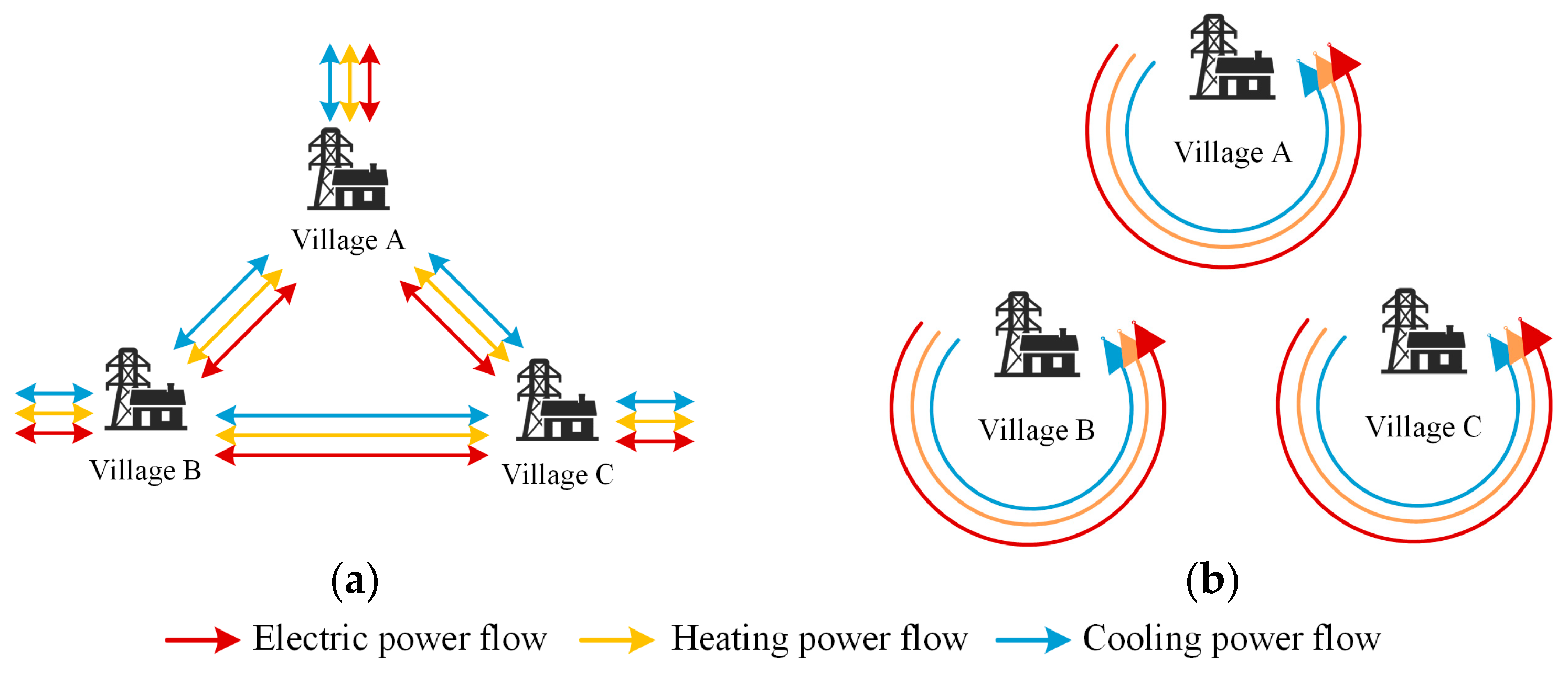
The MV-RMEG system constructed in this study extends its coverage from a single village to multiple villages. This enables coordinated mutual support among neighboring villages. The operational framework is illustrated in Figure 2.
As depicted in Figure 2a, each rural area is in a normal state of energy exchange with the external electricity, heating, and cooling network. Under these conditions, the individual RMEGs aggregate into a larger, integrated MV-RMEG. This leverages the distinct characteristics of each village’s energy equipment and load profile to achieve system-wide optimal operation across the interconnected villages. This approach avoids resource wastage stemming from duplicate investments and redundant equipment capacity.
Compared to urban systems, rural energy systems exhibit greater vulnerability. As shown in Figure 2b, when energy exchange between villages and the external grid is interrupted, and inter-village connections are lost, each village relies solely on its local energy resources to ensure the operation of critical loads over a specific period. Consequently, the system is endowed with autonomous functions from the planning stage, significantly enhancing its resilience against operational risks.
Under the vigorous advancement of comprehensive rural revitalization, modern villages are often endowed with diverse functionalities, emphasizing characteristics such as residential areas, agricultural production, and animal husbandry. Based on the industrial positioning and load characteristics of villages, this article considers the differences in energy equipment between villages during the planning stage. For any village m ∈ [1, M], ζ is adopted to denote the energy form of electricity, heating, or cooling. In the collaborative state, we have the following:
j m ζ j , m ( t ) = m ζ m load ( t )
where ζj,m(t) is the total power output of equipment j in village m, and ζ m load ( t ) is the total load of village m.
The rural power grid is relatively weak. When the external power supply is cut off, the connections between different villages are severed, resulting in an isolated operation state. This study further incorporates the autonomous constraints of each village into the planning model, ensuring that the planned equipment within each village can provide the energy supply for the critical loads in off-grid situations. The energy support that various equipment can provide is defined as follows:
P w , sup = m e a n N w P ¯ w ( t ) P pv , sup = m e a n N pv P ¯ pv ( t ) P ev , sup = N pile P ¯ dis P mt , sup = P ¯ mt
Q ashp , sup = P ¯ ashp η ashp , h Q mt , sup = P ¯ mt 1 η mt , e η hl η whr , r η whr , h η mt , e Q bb , sup = Q ¯ bb
C ashp , sup = P ¯ ashp η ashp , c C ac , sup = Q ¯ ac η ac
where mean[·] represents the calculation of the mean value. In the autonomous state, for any type of energy source, the energy supply within a single village can meet the critical load demands of the village itself.
j ζ j , m sup = θ m load m a x t ζ m load ( t )
where ζ j , m sup represents the energy support provided by equipment j within village m, and θ m load represents the proportion of critical loads in village m.

3.2. MV-RMEG Planning Model

Traditional RMEG planning models focus solely on single, isolated systems and employ fixed load parameters as the data foundation for planning. This study expands the scope to encompass multiple neighboring villages. This approach leverages the distinctive characteristics of each participating village, fostering collaborative complementarity in energy coupling while simultaneously ensuring the capability to maintain critical internal loads during disconnection from the external grid. Furthermore, the model incorporates the annual growth of both general load and EV penetration throughout the entire planning horizon, thereby enhancing the feasibility of the planning results.
The overall objective function for MV-RMEG planning in this study comprises four key cost components—investment cost, operation and maintenance cost, DG curtailment cost, and environmental cost—which can be expressed as
F obj = F inv + F om + F cur + F env
The decision variables representing the planning capacity for each equipment are expressed in a set form as
Ω = N w P w , rate , N pv P pv , rate , N pile P ch , P ¯ mt , Q ¯ bb , P ¯ ashp , Q ¯ ac
where Nw and Npv represent the number of WTs and PV panels, respectively. The investment cost is the sum of the initial investment expenses of all energy equipment in the MV-RMEG, which is related to each equipment’s planned capacity ωj ∈ Ω.
F inv = j λ j inv ω j r 1 + r y j 1 + r y j 1
where ωj, yi, and λ j inv represent the planned capacity, planned years, and investment cost per unit capacity of equipment j, respectively. r is the discount rate.
The operation and maintenance cost is related to the utilization rate of each equipment and the power purchased from the grid, which can be calculated as follows:
F om = 1 y pla j k y t T k λ j om R j , y , k ( t ) Δ t + T k λ t e P y , k grid ( t ) Δ t
where ypla represents the planning period calculated during the optimization process. Tk is the number of days a typical day k represents in a year. λ j om is the operation and maintenance cost of equipment j. Rj,y,k(t) is the electric/heating/cooling power of equipment j at time t in a typical day k of year y. λ t e is the time-of-use electricity price, and Δt is the length of each time slot.
The DG curtailment cost refers to the portion of WT and PV power that is not consumed. To encourage the local consumption of DG, this study does not consider the reverse transmission from DG to the grid.
F cur = 1 y pla k y t T k λ cur × P ¯ y , k w ( t ) P y , k w ( t ) + P ¯ y , k pv ( t ) P y , k pv ( t ) Δ t
where λcur represents the cost coefficient for DG curtailment. P k , y w ( t ) and P k , y pv ( t ) represent the actual output of WT and PV at time t in a typical day k of year y.
The environmental cost is defined as the difference between the actual emission cost and the emissions reduction benefit. The calculation method for the emission cost is mathematically defined in Equation (39). It encompasses the environmental costs of pollutants generated from grid power purchases and biogas combustion. Conversely, the calculation method for the reduction benefit is given by Equation (40), which represents the reduced cost of manure pollution due to biogas utilization.
F env = F env , pro F env , red
F env , pro = 1 y pla l k y t T k λ l pol × θ l e P y , k grid ( t ) + θ l met V y , k mt ( t ) + V y , k bb ( t ) Δ t
F env , red = 1 y pla l k y t λ l pol θ l mat V y , k mt ( t ) + V y , k bb ( t ) V met
where λ l pol is the environmental cost coefficient of pollutant l. θ l e / met represents the emissions of pollutant l generated per kWh of electricity and per cubic meter of biogas combustion, respectively. θ l mat is the emission of pollutant l produced by livestock manure daily.
The equality constraints include the balance equations for electricity, heat, and cooling power. This paper does not consider the reverse power flow between the point of common coupling (PCC) and the power grid, meaning that the MV-RMEG can only purchase electricity from the power grid.
P w ( t ) + P pv ( t ) + P mt ( t ) + P grid ( t ) = P load ( t ) + P ashp ( t ) + P station ( t )
Q bb ( t ) + Q whr ( t ) + Q ashp ( t ) = Q load ( t )
C ac ( t ) + C ashp ( t ) = C load ( t )
The inequality constraints include the upper limit constraints for each component’s power within the MV-RMEG.
0 P pv ( t ) N pv P ¯ pv ( t )
0 P grid ( t ) P ¯ grid
0 P w ( t ) N w P ¯ w ( t )
0 P mt ( t ) P ¯ mt
0 Q bb ( t ) Q ¯ bb

4. IGDT-Based Uncertainty Handling Method for MV-RMEG

4.1. IGDT Method

The optimization scenario in the aforementioned modeling process is based on fixed typical days. In reality, the stochastic nature of DG output and load is significant, necessitating consideration of the impacts caused by uncertainties. This study introduces IGDT into the MV-RMEG planning to address uncertainties. IGDT typically encompasses two strategies: risk-averse and opportunity-seeking. To mitigate the adverse effects induced by uncertainties in long-term planning, this study adopts the risk-averse IGDT strategy.
Firstly, the uncertainty sets are formulated to be centered on a typical day’s forecasted data. A fractional error approach is used to form the uncertainty model [35]. The uncertain radius, a crucial parameter of the uncertainty sets, characterizes the degree of deviation from the typical day data and determines the size of the set. The formulated uncertainty sets are as follows:
Ω ψ pv , P ˜ pv ( t ) = P ¯ pv ( t ) : P ¯ pv ( t ) P ˜ pv ( t ) P ˜ pv ( t ) ψ pv Ω ψ w , P ˜ w ( t ) = P ¯ w ( t ) : P ¯ w ( t ) P ˜ w ( t ) P ˜ w ( t ) ψ w Ω ψ load , P ˜ load ( t ) = P ¯ w ( t ) : P ¯ load ( t ) P ˜ load ( t ) P ˜ load ( t ) ψ load   ψ pv 0   ,   ψ w 0   ,   ψ load 0
where Ω is an uncertainty set; ψpv, ψw, and ψload are the uncertain radii of PV output, WT output, and load, respectively; and P ˜ pv ( t ) , P ˜ w ( t ) , and P ˜ load ( t ) are the corresponding predicted values. On this basis, the uncertain radii are expressed in an integrated form as follows:
ψ = λ pv ψ pv + λ w ψ w + λ load ψ load
where ψ represents the integrated uncertain radius. λpv, λw, and λload are the weight coefficients for uncertain radii.
Under the risk-averse IGDT strategy, decision-makers consider the adverse effects of uncertainties and allow the total cost to increase to a certain extent. Therefore, the optimized planning scheme can be conservative in dealing with the worst scenario of uncertain variables. The IGDT aims to seek the maximum uncertainty radius while controlling the growth range of the overall cost. The IGDT strategy model is constructed as follows [36]
max ψ s . t . max F obj 1 + π F ˜ obj P ¯ pv ( t ) Ω ψ pv , P ˜ pv ( t ) P ¯ w ( t ) Ω ψ w , P ˜ w ( t ) P ¯ load ( t ) Ω ψ load , P ˜ load ( t ) 1 32 , 41 50
where π represents the robust factor. Decision-makers can regulate the robustness of the planning scheme by adjusting the value of π. When π is set to 0, the model returns to a deterministic optimization model based on predicting DG output and load data. F ˜ obj is the objective function value obtained by optimizing the predicted data in typical days. We can observe that the model has a two-layer structure for maximizing, which is difficult to solve directly. According to the model presented in Section 3, it can be observed that the cost increases as the DG output decreases and the load rises. Therefore, the two-layer optimization in Equation (51) can be transformed into a single-layer optimization form [37]
max ψ s . t . F obj 1 + π F ˜ obj P ¯ pv ( t ) = 1 ψ pv P ˜ pv ( t ) P ¯ w ( t ) = 1 ψ w P ˜ w ( t ) P ¯ load ( t ) = 1 + ψ load P ˜ load ( t ) 1 32 , 41 48 , 50
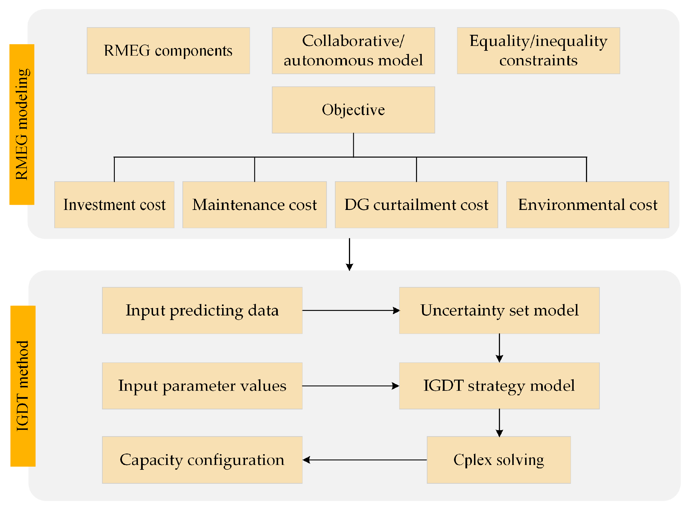
The planning scheme for the MV-RMEG is finally obtained by optimizing Equation (52). The flowchart of the overall planning method is shown in Figure 3.

4.2. Solution Method

The established mixed-integer second-order cone programming (MISOCP) model can be programmed in Matlab R2022a and directly solved by Cplex 12.10 through the Yalmip R20230622 toolbox.
Yalmip is an optimization modeling toolbox in the MATLAB environment, which supports the unified construction of various types of problems, such as linear programming, quadratic programming, and integer programming, through a concise declarative syntax. It can automatically convert the model into a standard format, significantly reducing the modeling difficulty of complex optimization problems.
Cplex, developed by IBM as a high-performance mathematical programming solver, relies on advanced algorithms such as branch and bound, cutting planes, etc., and can efficiently handle large-scale and highly complex linear and integer programming problems. It is widely used in engineering optimization and operations research fields. The combination of the two can fully leverage the advantages of convenient modeling and efficient solving, providing technical support for the reliable solution of optimization problems in research [33].
The average solution time on a laptop with a Core i7-12700H CPU and 16GB RAM is 5 min and 30 s. Since the paper focuses on the long-term planning problem, the impact of computation time can be considered negligible.

5. Case Studies

This section conducts simulation verification of the proposed model and method. Firstly, we introduce the parameter settings used in the simulation. Then, the capacity configuration of RMEG is presented. Based on the capacity, the operation performance under typical days is discussed. Moreover, we test the superiority of collaborative and autonomous modes, as well as the impact brought about by allowing bidirectional power flow at the PCC. Finally, we modify the key parameter values in IGDT to evaluate their impact on the proposed method.

5.1. Parameter Settings

This section presents the simulation verification of the proposed model and method. The simulation takes a rural area in the North China Plain as an example, involving three adjacent villages. Village A focuses on residential housing and tourism, Village B specializes in large-scale breeding, and Village C primarily engages in facility agriculture with PV complementation. The types of energy equipment available in each village are detailed in Table 2. Based on meteorological data from Beijing, the number of days for spring, summer, autumn, and winter within a year is 55, 116, 48, and 146 days, respectively. The parameters related to the breeding scale and biogas production are provided in Table 3. The environmental cost coefficients for CH4, N2O, and biogas combustion are set at 2.9 USD/kg, 49.6 USD/kg, and 0.01 USD/kg, respectively. The typical daily profiles of historical solar irradiance and wind speed records sourced from NASA’s open data [38] are shown in Figure 4. The temperature for typical days and the electricity price are shown in Figure 5. A base load growth over 10 years is considered in the simulation. EVs are modeled using the BYD Qin Plus equipped with a 57.6 kWh power battery. The growth rate of the EV population is derived by fitting the baseline forecast data obtained from reference [39]. Other relevant parameters are specified in Table 4.

5.2. Planning Scheme and Result Analysis

Under the proposed method, the long-term planning scheme for the capacities of key equipment is presented in Table 5. The table shows that the planning process leverages rural characteristics by fully utilizing local natural resources such as wind, solar, and biomass for energy supply. The study area has distinct seasons, with low temperatures, short daylight hours, and substantial nighttime heating loads in winter. Therefore, the planned capacity of a WT is 4940 kW higher than that of a PV. Considering the substantial daily manure output from large-scale breeding operations, the total capacity of micro gas turbines and biogas boilers is configured as 6580 kW to meet the energy demands of the three villages. Additionally, 64 fast-charging piles are installed to cater to the EV charging needs of both rural residents and tourists.
The simulation results of the electrical load for typical days across different seasons are shown in Figure 6. The vertical axis in the figure is divided into two directions. The upward direction represents the power supply, while the downward direction represents the consumption of various loads. Regarding load composition, the cooling load in summer and the heating load in winter constitute a high proportion, resulting in a significantly increased electrical load due to ASHP operation. Regarding power generation, grid purchases account for only 0.24% of the annual load demand. The three villages basically achieved self-sufficiency in electricity supply by relying on renewable energy throughout the year. PV generation is fully utilized during daytime, while WT and biogas power generation dominate the nighttime supply. Furthermore, PV generation in North China during winter is constrained by low temperatures and low solar irradiance, contributing only 4.35% to the total demand. Consequently, even during the daytime, wind power and biogas power generation serve as the primary power supply.
The heating demand in winter and in summer differs significantly, resulting in pronounced fluctuations in the heating load. As shown in Figure 7, the peak heating load in winter reaches 5.83 times that in summer. Consequently, the structures for heating supply exhibit distinct patterns between these two seasons. The figure indicates that biogas boilers and waste heat recovery units are the heating sources in spring, summer, and autumn. In winter, however, 83.51% of the biogas is utilized by gas turbines to compensate for the reduction in PV output. Only 16.49% of the biogas is allocated for heat production, as ASHPs displace biogas boilers to become the primary supply for winter heating.
Figure 8 shows the variation in the cooling system in each season. Affected by temperature, the cooling and heating demand trends in winter and summer are opposite to each other. The peak cooling demand of summer is 3.96 times that of winter. In spring, summer, and autumn, ASHPs undertake the cooling task. In winter, however, ASHPs operate primarily in the heating mode, supplying only 35.89% of the total cooling demand. ACs meet the remaining 64.11%.

5.3. Analysis of Collaborative/Autonomous Operation Framework

To verify the economic and operational performance of the proposed strategy, we simulated four alternative planning methods for comparative analysis.
Case 1: Neither the collaborative mode nor the autonomous mode is considered during planning.
Case 2: Only the autonomous mode is considered during the planning process.
Case 3: Only the collaborative mode is considered during the planning process.
Case 4: The proposed strategy, which considers both the collaborative mode and the autonomous mode.
Case 5: The proposed strategy. However, the MV-RMEG can conduct bidirectional power flow interaction with the power grid through the PCC.
The simulation results are presented in Table 6. As we can see, the proposed strategy exhibits the highest investment cost in the first four cases due to its simultaneous integration of both modes. Case 1 shows a 328,660 USD reduction in annualized investment cost and a 6110 USD reduction in DG curtailment cost compared to the proposed method. However, the lower capacity configuration of DGs and gas turbines in case 1 leads to a substantially higher power purchasing cost, exceeding case 4 by 677,420 USD. To evaluate off-grid performance, the three villages were set as disconnected from the grid from 10:00 to 15:00. Owing to the consideration of autonomous operation, the shedding rate for critical load in the proposed strategy achieves only 3.96%, which is 27.27% lower than case 1. Furthermore, case 2 demonstrates a 23.83% lower load shedding rate than case 3, further proving that considering autonomous operation in the model can effectively enhance critical load supply during islanding. Case 3 does not incur power purchasing cost, proving that the collaborative mode maximizes the energy coupling advantages of the MV-RMEG. Case 5 allows the PCC to have bidirectional power flow, which is beneficial for selling the excess DG output to the grid. It can be seen that the curtailment cost has been further reduced. The investment cost increases by 3.59% compared to case 4, indicating that the planning scheme leans towards building more DG to gain benefits. Additionally, all methods yield significant environmental benefits through utilizing livestock manure and substituting renewable energies for traditional generation. This comprehensive comparison confirms that the proposed strategy delivers optimal total costs, demonstrating superior performance in reducing power purchases and ensuring off-grid power supply reliability.

5.4. Analysis of the IGDT Planning Method

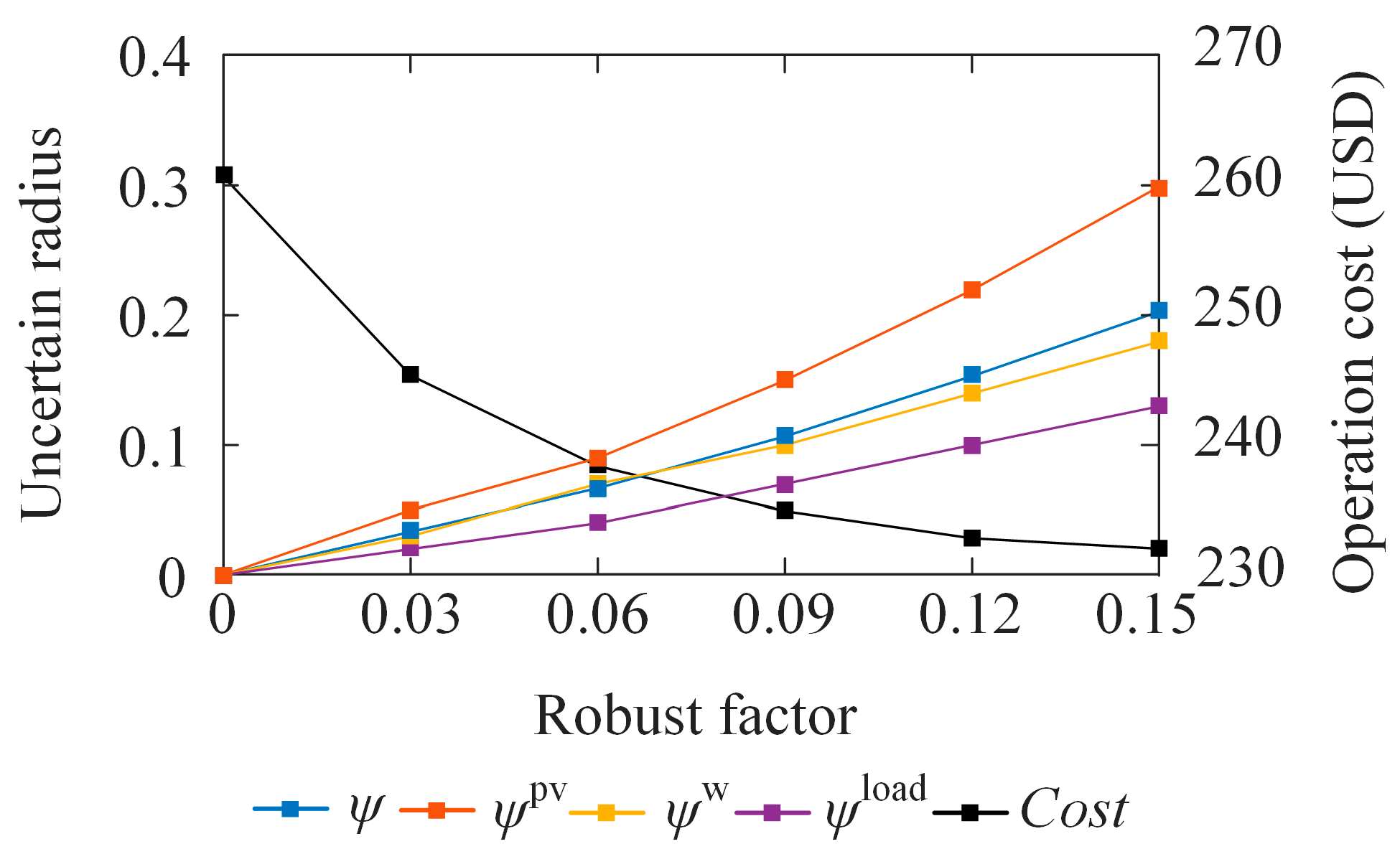
In the proposed MV-RMEG planning method, the robust factor and weight coefficients for uncertain radii are critical for addressing uncertainties. When the robust factor π varies between 0 and 0.15, the solution results of IGDT show a trajectory as depicted in Figure 9. It is evident that the uncertain radii demonstrate a positive correlation with π. This occurs because an increase in π elevates the total planning cost under IGDT, necessitating larger uncertain radii to accommodate more adverse DG output conditions. A comparative analysis reveals that the uncertainty radius of PV exceeds that of WT. This indicates that PV fluctuations exert a comparatively smaller impact on MV-RMEG planning. This phenomenon primarily stems from the selected region’s shorter daylight hours and lower temperatures during winter. Consequently, the results demonstrate that the MV-RMEG exhibits greater sensitivity to the adverse conditions of WT output. In contrast, the impact of load is much more profound than that of DG. The proposed method is compared with the deterministic optimization method based on predicting information (i.e., π = 0). Monte Carlo simulation (MCS) is used to randomly generate forty scenarios of DG output and load. The daily operation cost is tested with different values of π. As shown in the figure, the overall operating cost decreases as π increases. The deterministic method fails to take into account the possible random fluctuations. Therefore, the planning result is overly aggressive, resulting in excessively high costs. However, when the π is too high, it will result in redundant capacity of the RMEG equipment, leading to a convergence in costs.
In the above simulations, the weight coefficients for the uncertain radii of PV, WT, and load were both set to 0.33. Table 7 compares the IGDT planning results when these weights have been modified, revealing that when a specific DG’s uncertain radius receives a higher weight, the corresponding capacity configuration and curtailment cost decrease accordingly. Taking PV as an example, when the weight increases from 0.33 to 0.6, its investment cost and curtailment cost are reduced by 29.94% and 27.37%, respectively. This is because the objective function aims to maximize the integrated uncertain radius. After λpv increases, more severe scenarios of PV fluctuations will be taken into account during the planning process. Consequently, the MV-RMEG improves its robustness against PV uncertainty by reducing the capacity configuration.

6. Conclusions

This study proposes a planning method for MV-RMEGs tailored to multiple villages’ synergistic supply–demand scenarios. Building upon a coupled model integrating rural renewable energy supply and load carrying, the proposed method incorporates the collaborative/autonomous framework in both off-grid and grid-connected states, while accounting for uncertainties in DG output.
The proposed MV-RMEG framework breaks through the current widely adopted single-village planning approach. By comparing it with the single-village planning schemes, the proposed method reduces the power purchasing cost by 99.61%. This depends on the ability of MV-RMEG to integrate the resources of each village. During periods when the external energy supply is cut off in each village, the crucial load supply rate of MV-RMEG is also 27.27% higher than that of the single-village mode. Furthermore, the proposed IGDT method performs well in handling the uncertainties present in MV-RMEG. Compared with deterministic optimization, the proposed method reduces the operation cost by 10.25%, which demonstrates better robustness in various uncertain scenarios.

Author Contributions

Conceptualization, Y.W.; methodology, X.L.; software, Y.W., X.L., and Z.Z.; validation, Z.Z. and G.L.; formal analysis, G.L. and X.L.; investigation, Y.Z.; resources, Y.Z.; data curation, G.M.; writing—original draft preparation, Y.W. and P.W.; writing—review and editing, Z.W.; visualization, G.M.; supervision, P.W.; project administration, Z.W.; funding acquisition, Z.W. All authors have read and agreed to the published version of the manuscript.

Funding

This research was funded by the Science and Technology Project of State Grid Hebei Electric Power Co., Ltd. (Grant No. kj2024-020).

Data Availability Statement

The original study’s contributions are included in this article, and any further inquiries can be directed to the corresponding authors.

Conflicts of Interest

Authors Yunjia Wang, Xuefei Liu, Zeya Zhang, Guangyi Li, Yan Zhang, Guozhen Ma were employed by the company Economic and Techology Research Institute, State Grid Hebei Electric Power Co., Ltd. The remaining authors declare that the research was conducted in the absence of any commercial or financial relationships that could be construed as a potential conflict of interest. The company had no role in the design of the study; in the collection, analyses, or interpretation of data; in the writing of the manuscript, or in the decision to publish the results.

Abbreviations

The following abbreviations are used in this manuscript:
RMEGRural micro-energy grid
MV-RMEGMulti-village coupled rural micro-energy grid
DGDistributed generation
IGDTInformation gap decision theory
EVElectric vehicle
ASHPAir-source heat pump
PVPhotovoltaic
WTWind turbine
ACAbsorption chiller
CHPCombined heat and power

References

  1. Wang, Q.; Xiao, Y.; Tan, H.; Mohamed, M.A. Day-Ahead Scheduling of Rural Integrated Energy Systems Based on Distributionally Robust Optimization Theory. Appl. Therm. Eng. 2024, 246, 123001. [Google Scholar] [CrossRef]
  2. National Energy Administration. Guiding Opinions on Promoting the Transformation and Development of Rural Energy to Support Rural Revitalization. Available online: https://www.gov.cn/zhengce/zhengceku/2022-01/07/content_5666809.htm (accessed on 31 July 2025).
  3. Wang, Y.; Jin, J.; Liu, H.; Zhang, Z.; Liu, S.; Ma, J.; Gong, C.; Zheng, Y.; Lin, Z.; Yang, L. The Optimal Emergency Demand Response (EDR) Mechanism for Rural Power Grid Considering Consumers’ Satisfaction. Energy Rep. 2021, 7, 118–125. [Google Scholar] [CrossRef]
  4. Chawda, G.S.; Shaik, A.G. Power Quality Improvement in Rural Grid Using Adaptive Control Algorithm to Enhance Wind Energy Penetration Levels. IEEE Trans. Smart Grid 2023, 14, 2075–2084. [Google Scholar] [CrossRef]
  5. Yang, S.; Fang, J.; Zhang, Z.; Lv, S.; Lin, H.; Ju, L. Two-Stage Coordinated Optimal Dispatching Model and Benefit Allocation Strategy for Rural New Energy Microgrid. Energy 2024, 292, 130274. [Google Scholar] [CrossRef]
  6. Li, P.; Zhao, M.; Zhang, H.; Zhang, O.; Li, N.; Yue, X.; Tan, Z. An Operational Optimization Model for Micro Energy Grids in Photovoltaic-Storage Agricultural Greenhouses Based on Operation Mode Selection. Processes 2025, 13, 1622. [Google Scholar] [CrossRef]
  7. Wang, Y.; Guo, L.; Ma, Y.; Han, X.; Xing, J.; Miao, W.; Wang, H. Study on Operation Optimization of Decentralized Integrated Energy System in Northern Rural Areas Based on Multi-Objective. Energy Rep. 2022, 8, 3063–3084. [Google Scholar] [CrossRef]
  8. Liu, Y.; Xu, X.; Liu, Y.; Liu, J.; Hu, W.; Yang, N.; Jawad, S.; Wei, Z. Operational Optimization of a Rural Multi-Energy System Supported by a Joint Biomass-Solid-Waste-Energy Conversion System and Supply Chain. Energy 2024, 312, 133528. [Google Scholar] [CrossRef]
  9. Ju, L.; Lv, S.; Zhang, Z.; Li, G.; Gan, W.; Fang, J. Data-Driven Two-Stage Robust Optimization Dispatching Model and Benefit Allocation Strategy for a Novel Virtual Power Plant Considering Carbon-Green Certificate Equivalence Conversion Mechanism. Appl. Energy 2024, 362, 122974. [Google Scholar] [CrossRef]
  10. Li, W.; Zou, Y.; Yang, H.; Fu, X.; Xiang, S.; Li, Z. Two-Stage Stochastic Energy Scheduling for Multi-Energy Rural Microgrids With Irrigation Systems and Biomass Fermentation. IEEE Trans. Smart Grid 2025, 16, 1075–1087. [Google Scholar] [CrossRef]
  11. Han, F.; Zhao, Y.; Zeng, J.; Zhang, S.; Wu, T. Uncertain Parameters Adjustable Two-Stage Robust Optimization of a Rural Housing Integrated Energy System Considering Biomass on-Site Utilization. Energy 2024, 296, 131106. [Google Scholar] [CrossRef]
  12. Wu, S.; Wang, Y.; Liu, L.; Yang, Z.; Cao, Q.; He, H.; Cao, Y. Two-Stage Distributionally Robust Optimal Operation of Rural Virtual Power Plants Considering Multi Correlated Uncertainties. Int. J. Electr. Power Energy Syst. 2024, 161, 110173. [Google Scholar] [CrossRef]
  13. Ugwoke, B.; Sulemanu, S.; Corgnati, S.P.; Leone, P.; Pearce, J.M. Demonstration of the Integrated Rural Energy Planning Framework for Sustainable Energy Development in Low-Income Countries: Case Studies of Rural Communities in Nigeria. Renew. Sustain. Energy Rev. 2021, 144, 110983. [Google Scholar] [CrossRef]
  14. Liu, W.; Gao, X.; Liu, C.; Shi, Q. Reliability-Constrained Bi-Level Collaborative Planning of Distribution Network and Micro-Energy Grid. Int. J. Electr. Power Energy Syst. 2023, 152, 109199. [Google Scholar] [CrossRef]
  15. Wang, Y.; Guo, L.; Wang, Y.; Zhang, Y.; Zhang, S.; Liu, Z.; Xing, J.; Liu, X. Bi-Level Programming Optimization Method of Rural Integrated Energy System Based on Coupling Coordination Degree of Energy Equipment. Energy 2024, 298, 131289. [Google Scholar] [CrossRef]
  16. Kumar, R.; Channi, H.K. A PV-Biomass off-Grid Hybrid Renewable Energy System (HRES) for Rural Electrification: Design, Optimization and Techno-Economic-Environmental Analysis. J. Clean. Prod. 2022, 349, 131347. [Google Scholar] [CrossRef]
  17. Chen, M.; Wei, J.; Yang, X.; Fu, Q.; Wang, Q.; Qiao, S. Multi-Objective Optimization of Multi-Energy Complementary Systems Integrated Biomass-Solar-Wind Energy Utilization in Rural Areas. Energy Convers. Manag. 2025, 323, 119241. [Google Scholar] [CrossRef]
  18. Abazari, A.; Soleymani, M.M.; Kamwa, I.; Babaei, M.; Ghafouri, M.; Muyeen, S.M.; Foley, A.M. A Reliable and Cost-Effective Planning Framework of Rural Area Hybrid System Considering Intelligent Weather Forecasting. Energy Rep. 2021, 7, 5647–5666. [Google Scholar] [CrossRef]
  19. Li, X.; Zhang, L.; Wang, R.; Sun, B.; Xie, W. Two-Stage Robust Optimization Model for Capacity Configuration of Biogas-Solar-Wind Integrated Energy System. IEEE Trans. Ind. Appl. 2023, 59, 662–675. [Google Scholar] [CrossRef]
  20. Li, S.; Zhang, L.; Wang, X.; Zhu, C. A Decision-Making and Planning Optimization Framework for Multi-Regional Rural Hybrid Renewable Energy System. Energy Convers. Manag. 2022, 273, 116402. [Google Scholar] [CrossRef]
  21. Zhang, L.; Chen, A.; Gu, H.; Wang, X.; Xie, D.; Gu, C. Planning of the Multi-Energy Circular System Coupled with Waste Processing Base: A Case from China. Energies 2019, 12, 3910. [Google Scholar] [CrossRef]
  22. Ju, L.; Lu, X.; Yang, S.; Li, G.; Fan, W.; Pan, Y.; Qiao, H. A Multi-Time Scale Dispatching Optimal Model for Rural Biomass Waste Energy Conversion System-Based Micro-Energy Grid Considering Multi-Energy Demand Response. Appl. Energy 2022, 327, 120155. [Google Scholar] [CrossRef]
  23. Fu, X.; Wei, Z.; Sun, H.; Zhang, Y. Agri-Energy-Environment Synergy-Based Distributed Energy Planning in Rural Areas. IEEE Trans. Smart Grid 2024, 15, 3722–3738. [Google Scholar] [CrossRef]
  24. Liu, Y.; Xu, X.; Xu, L.; Liu, Y.; Liu, J.; Hu, W.; Yang, N.; Jawad, S.; Luo, Y. Multi-Timescale Collaborative Operation of Renewable Energy-Based Power System and Agri-Product Supply Chain Considering Dynamic Energy Consumption-Based Crop Growth. Appl. Energy 2025, 377, 124359. [Google Scholar] [CrossRef]
  25. Jiang, M.; Xu, Y.; Zhang, D.; Liu, Y.; Du, Q.; Gao, X.; Qi, S.; Zou, H. Research on an Active Distribution Network Planning Strategy Considering Diversified Flexible Resource Allocation. Processes 2025, 13, 2254. [Google Scholar] [CrossRef]
  26. Liang, H.; Yu, L.; Yan, L.; Han, J. Design of Micro-Grid with Biogas Power Generation. In Proceedings of the International Conference on Renewable Power Generation (RPG 2015), Beijing, China, 17–18 October 2015; Institution of Engineering and Technology: Hong Kong, China, 2015; p. 5. [Google Scholar]
  27. Wang, R.; Wang, J. Multi-Objective Collaborative Optimization of System Configurations and Energy Scheduling of Integrated Energy System with Electricity-Fuel-Heat Storage Systems. J. Energy Storage 2025, 132, 117846. [Google Scholar] [CrossRef]
  28. Sun, L.; Hu, Z.; Mae, M.; Imaizumi, T. A Predictive COP Model for Air Source Heat Pumps under Extreme Heat Conditions Using No Experimental Data. Energy Build. 2025, 339, 115749. [Google Scholar] [CrossRef]
  29. Liu, Z.; Liu, X.; Wu, D.; Jin, G.; Fan, G.; Guo, J.; Xu, H. Multi-Time-Scale Optimization Method Based on an Integrated Cooperative Cooling, Heating, and Electricity Storage Supply System. J. Energy Storage 2025, 122, 116592. [Google Scholar] [CrossRef]
  30. Habash, R.; Gediz ilis, G.; Ünal, Ş.; Saha, B.B. Enhancing COP of Electric Vehicle Cooling Systems Using Adsorption Heat Pumps. Therm. Sci. Eng. Prog. 2025, 64, 103788. [Google Scholar] [CrossRef]
  31. Chen, X.; Leung, K.C. Non-Cooperative and Cooperative Optimization of Scheduling with Vehicle-to-Grid Regulation Services. IEEE Trans. Veh. Technol. 2020, 69, 114–130. [Google Scholar] [CrossRef]
  32. Wu, C.; Gao, S.; Liu, Y.; Song, T.E.; Han, H. A Model Predictive Control Approach in Microgrid Considering Multi-Uncertainty of Electric Vehicles. Renew. Energy 2021, 163, 1385–1396. [Google Scholar] [CrossRef]
  33. Topa, A.O.; Gil, J.D.; Álvarez, J.D.; Torres, J.L. A Hybrid-MPC Based Energy Management System with Time Series Constraints for a Bioclimatic Building. Energy 2024, 287, 129652. [Google Scholar] [CrossRef]
  34. Li, M.; Liu, Q.; Zhao, G.; Zhou, B.; Xia, H.; Zang, T. Rural Integrated Energy System Planning Considering Multi-Industry Synergy. Zhongguo Dianli/Electr. Power 2022, 55, 14–22. [Google Scholar] [CrossRef]
  35. Van Phu, P.; Huy, T.H.B.; Park, S.; Kim, D. An IGDT Approach for the Multi-Objective Framework of Integrated Energy Hub with Renewable Energy Sources, Hybrid Energy Storage Systems, and Biomass-to-Hydrogen Technology. J. Energy Storage 2024, 89, 111488. [Google Scholar] [CrossRef]
  36. Cao, X.; Wang, J.; Zeng, B. A Chance Constrained Information-Gap Decision Model for Multi-Period Microgrid Planning. IEEE Trans. Power Syst. 2018, 33, 2684–2695. [Google Scholar] [CrossRef]
  37. Liao, S.; Liu, H.; Liu, B.; Zhao, H.; Wang, M. An Information Gap Decision Theory-Based Decision-Making Model for Complementary Operation of Hydro-Wind-Solar System Considering Wind and Solar Output Uncertainties. J. Clean. Prod. 2022, 348, 131382. [Google Scholar] [CrossRef]
  38. NASA. NASA Power. Available online: https://power.larc.nasa.gov/data-access-viewer/ (accessed on 31 July 2025).
  39. China EV100 Research on the Development of Electric Vehicles in China’s Rural Areas. Available online: http://www.nrdc.cn/Public/uploads/2020-07-17/5f1125d5ac64d.pdf (accessed on 31 July 2025).
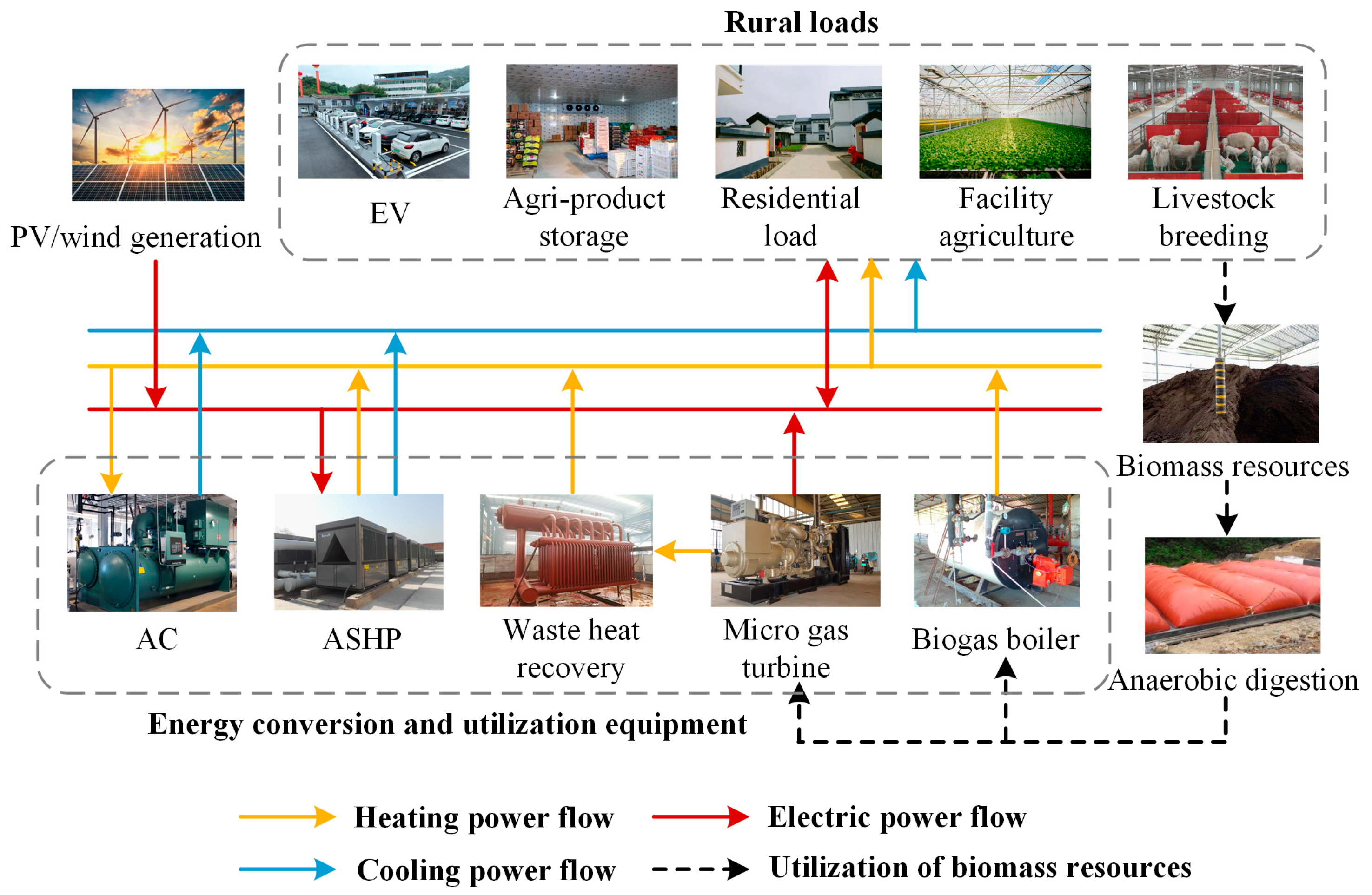
Figure 1. Structure diagram of MV-RMEG.
Processes 13 02881 g001
Figure 2. Collaborative/autonomous operation framework for MV-RMEG: (a) collaborative state; (b) autonomous state.
Processes 13 02881 g002
Figure 3. Flowchart of the proposed planning method.
Processes 13 02881 g003
Figure 4. Variation in irradiance and wind speed on typical days.
Processes 13 02881 g004
Figure 5. Variation in temperature and electricity price on typical days.
Processes 13 02881 g005
Figure 6. Comparison of electrical system output on typical days in (a) spring and autumn; (b) summer; and (c) winter.
Processes 13 02881 g006
Figure 7. Comparison of heating system output on typical days in (a) spring and autumn; (b) summer; and (c) winter.
Processes 13 02881 g007
Figure 8. Comparison of cooling system output on typical days in (a) spring and autumn; (b) summer; and (c) winter.
Processes 13 02881 g008
Figure 9. IGDT results under robustness factor variation.
Processes 13 02881 g009
Table 1. Literature review and the state of the art of RMEG planning studies.
ReferenceRMEG AreaOptimization Approach
Ref. [16]Single-villageDeterministic optimization with historical data
Ref. [17]Single-villageDeterministic optimization with historical data
Ref. [18]Single-villageDeterministic optimization with predicting data based on fuzzy c-means clustering technique
Ref. [19]Single-villageTwo-stage robust optimization
Ref. [20]Single-villageDeterministic optimization with historical data
Ref. [21]Single-villageDeterministic optimization with historical data
Ref. [22]Single-villageTwo-stage robust optimization
Ref. [23]Single-villageDeterministic optimization with historical data
Ref. [24]Single-villageDeterministic optimization with historical data
Table 2. Energy equipment configuration in each village.
EquipmentVillage AVillage BVillage C
PV
WT
Micro gas turbine
Biogas boiler
AC
ASHP
Charging piles
Table 3. Breeding scale and biogas production parameters.
ParametersPigsCattlePoultry
Breeding scale (animal)10,000300030,000
Daily manure excretion (kg/animal)2200.1
Gas production rate (m3/t)3617754
CH4 emission (kg/animal·day)1.4 × 10−22.28 × 10−25.48 × 10⁻⁵
N2O emission (kg/animal·day)4.93 × 10−45.67 × 10−32.74 × 10⁻⁵
Table 4. Simulation parameters.
ParametersUnitValue
Pw,ratekW100
Ppv,ratekW0.3
ηmt,e/hl/bb 0.35/0.5/0.9
ηwhr,r/whr,h 0.6/0.8
ηch/dis 0.9/0.9
μarr/dep 8/18
σarr/dep 1/1
EevkWh57.6
P ¯ ch / dis kW20/20
yplayear10
π 0.1
λpv/w/load 0.33
Table 5. Planning scheme for key equipment.
EquipmentCapacity (kW)
PV1560
WT6500
Charging piles1280
Micro gas turbine2430
Biogas boiler4150
ASHP in Village A1530
ASHP in Village C270
AC470
Table 6. Comparison of simulation results under different strategies.
EquipmentCase 1Case 2Case 3Case 4Case 5
Annualized investment cost (103 USD)908.29962.201145.791236.951281.3
Maintenance cost (103 USD)27.7621.3627.9427.5227.91
DG curtailment cost (103 USD)7.587.5413.9013.690
Power purchasing cost (103 USD)680.04701.220.012.621.88
Environmental cost (103 USD)−60.33−59.80−63.55−63.38−64.17
Load shedding rate during off-grid (%)31.2310.7334.563.963.43
Table 7. Comparison of IGDT results under different weight coefficients for uncertain radii.
λpvλwλloadAnnualized Investment Cost of PV (103 USD)Annualized Investment Cost of WT (103 USD)PV Curtailment Cost
(103 USD)
WT Curtailment Cost
(103 USD)
0.330.330.33131.85598.511.7911.9
0.60.20.292.37647.71.312.21
0.20.60.2176.23535.12.4311.62
0.20.20.6162.59580.332.2811.76
Disclaimer/Publisher’s Note: The statements, opinions and data contained in all publications are solely those of the individual author(s) and contributor(s) and not of MDPI and/or the editor(s). MDPI and/or the editor(s) disclaim responsibility for any injury to people or property resulting from any ideas, methods, instructions or products referred to in the content.