Article

Benchmarking ML Algorithms Against Traditional Correlations for Dynamic Monitoring of Bottomhole Pressure in Nitrogen-Lifted Wells

by
Samuel Nashed
* and
Rouzbeh Moghanloo
*
Mewbourne School of Petroleum and Geological Engineering, Mewbourne College of Earth and Energy, The University of Oklahoma, Norman, OK 73019, USA
*
Authors to whom correspondence should be addressed.
Processes 2025, 13(9), 2820; https://doi.org/10.3390/pr13092820
Submission received: 27 July 2025 / Revised: 18 August 2025 / Accepted: 1 September 2025 / Published: 3 September 2025
(This article belongs to the Section AI-Enabled Process Engineering)

Abstract

Proper estimation of flowing bottomhole pressure at coiled tubing depth (BHP-CTD) is crucial in optimization of nitrogen lifting operations in oil wells. Conventional estimation techniques such as empirical correlations and mechanistic models may be characterized by poor generalizability, low accuracy, and inapplicability in real time. This study overcomes these shortcomings by developing and comparing sixteen machine learning (ML) regression models, such as neural networks and genetic programming-based symbolic regression, in order to predict BHP-CTD with field data collected on 518 oil wells. Operational parameters that were used to train the models included fluid flow rate, gas–oil ratio, coiled tubing depth, and nitrogen rate. The best performance was obtained with the neural network with the L-BFGS optimizer (R2 = 0.987) and the low error metrics (RMSE = 0.014, MAE = 0.011). An interpretable equation with R2 = 0.94 was also obtained through a symbolic regression model. The robustness of the model was confirmed by both k-fold and random sampling validation, and generalizability was also confirmed using blind validation on data collected on 29 wells not included in the training set. The ML models proved to be more accurate, adaptable, and real-time applicable as compared to empirical correlations such as Hagedorn and Brown, Beggs and Brill, and Orkiszewski. This study does not only provide a cost-efficient alternative to downhole pressure gauges but also adds an interpretable, data-driven framework to increase the efficiency of nitrogen lifting in various operational conditions.

1. Introduction

1.1. The Significance of Predicting Flowing Bottomhole Pressure

Coiled tubing nitrogen lifting is widely applied in oil and gas wells to initiate or resume fluid production, particularly where a wellbore is full of completion or formation fluids that do not permit natural production. During this procedure, the nitrogen gas is injected through the coiled tubing in order to lower the hydrostatic pressure in the wellbore, thus enabling the reservoir fluids to flow into the well and move to the surface [1]. Nitrogen lifting works best when conditions in the downhole are well understood, especially the flowing bottomhole pressure at the coiled tubing depth (BHP-CTD). The real-time prediction of BHP-CTD is crucial to determine the optimum nitrogen injection rate and volume, adjusting the coiled tubing run-in-hole speed and depth [2]. It is also significant in avoiding operational problems like proppant flowback, sand production because of excessive pressure drawdown, or fluctuating flow rates because of inadequate drawdown [3]. BHP-CTD real-time estimation facilitates inflow performance relationships (IPR) assessment and allows making the informed decision in terms of whether artificial lift systems or stimulation treatment are necessary [4]. Without proper BHP-CTD forecasting, nitrogen lifting operations can be inefficient, which can lead to operational expenses, less well productivity, and increased safety hazards [5].

1.2. Traditional Prediction Methods

The conventional approaches to the prediction of flowing bottomhole pressure at coiled tubing depth are divided into three categories, such as empirical correlations, physics-based models, and unified models [6,7,8]. Empirical correlations are based on experimental data and field observations and give simplified mathematical expressions to estimate pressure drops [9,10]. Such procedures tend to be more convenient and less computationally intensive and may be appropriate for hand calculation or rough approximations [11,12,13]. But the main limitation is that their application is limited; their effectiveness decreases remarkably when they are used on a dataset or operating conditions that are not within the scope of development [14,15,16]. A single empirical correlation, or even a few correlations, is not reliable to predict pressure drop over the wide range of well conditions and multiphase flow regimes that are observed in the field [17]. Such a lack of universal validity can cause severe mistakes in forecasting, especially in dynamic and transient processes such as nitrogen lifting [18,19].
Mechanistic models are physics-based models, built on the basic principles of fluid mechanics and thermodynamics, and seek to explain the multiphase flow behavior in the wellbore [20,21]. These models give a good insight into the underlying physics and may be used to gain insight into complex flows [22,23]. But they are frequently constrained by many assumptions and simplifications, especially when extrapolated out of the laboratory and into the complex and diverse applications of multiphase flow in the field [24,25]. They also tend to need a large amount of input data and calibration and may be computationally intensive, thus being hard to apply in real-time in the field [26,27].
Unified models are special mechanistic tools that are aimed at predicting the behavior of multiphase flow under all pipe inclinations and flow conditions with the same physical framework [28,29]. The Barnea model is simple and fast, which makes it very helpful in making a quick field estimate and in academic research, but it is mostly empirical and less precise at high pressures or complex flow situations [30]. This is enhanced in the TUFFP unified model that has more complete slug flow dynamics and finer closure relationships, giving it more accuracy at a broader range of operating conditions, including three-phase systems [31]. Its drawback is that it is more complex to compute and requires specialized implementation, and this could limit its availability to general use [32]. The most sophisticated simulation features, such as transient modeling, are available in OLGA, and it is therefore very accurate in dynamic operations, such as nitrogen lifting. However, its intensive computation requirements, its steep learning curve, and high licensing fees may limit its application in real-time use [33,34].

1.3. Machine Learning Models for Predicting BHP

The conventional models of forecasting BHP-CTD have several shortcomings in terms of accuracy, as they are simplistic and limited in their application in different well conditions. These constraints leave a gap in reliable real-time BHP estimation, which may impede the efficiency of nitrogen lifting operations and slow down critical decisions [35]. A potentially more promising alternative is the use of machine learning (ML) regression models, which can find complex, non-linear relationships in large datasets without having to explicitly model the physical relationship [36,37,38,39]. Although there are major improvements in the use of data-driven methods in other fields of the oil and gas sector, including hydraulic fracturing [40,41], reservoir characterization [42,43,44,45], production forecasting [46,47,48], artificial lift systems [49,50,51], and completion design [52,53,54], the use of data-driven approaches to the specific issue of BHP prediction in nitrogen-lifted wells is underrepresented in the research [55,56]. More recent advances in ML, such as Genetic Programming-based Symbolic Regression (GPSR), which produces interpretable mathematical expressions, have started to alleviate some of the long-standing concerns about the lack of transparency and reliability of data-driven models [57,58]. Such innovations improve the feasibility and validity of ML methodologies in real-world conditions where the value of accuracy and interpretability are critical [59].
The presented paper is a unique contribution to the field because it provides a complete comparative study of different ML regression models, such as advanced neural networks and symbolic regression, specifically to predict BHP-CTD in vertical oil wells, based on a large dataset collected in 518 wells. In contrast to most of the literature that uses only one ML algorithm or synthetic data, this study provides a comparison of sixteen models using real operational parameters and provides an understanding of their relative performance, interpretability, and how they can be applied to a critical well intervention operation such as nitrogen lifting [60,61,62]. Moreover, they are more accurate and adaptable to a variety of field conditions and real-time compared to empirical correlations, physics-based models, and available unified models [63,64]. Machine learning models will require less time and cost relative to the widely used bottomhole pressure gauges, which can be very difficult to install [65]. Moreover, the explicit derivation and validation of a symbolic regression model provide an interpretable equation for BHP-CTD, enhancing transparency alongside predictive accuracy, whereas it could be said that a large dataset could be utilized instead to calibrate more robust physics-based models, the practice is hampered by the necessity to recalibrate a variety of empirical closure relationships, which tend to lack generalizability across a variety of flow regimes. In contrast, ML models are trained on data patterns directly, and once trained, have very low inference cost, as predictions can be made in terms of simple algebraic operations as opposed to iterative multiphase flow solvers. Such computational efficiency in combination with adaptability and scalability supports the practical benefit of the ML approach in real-time BHP prediction.

2. Methodology

The methodology that is used in this study has five different stages, as shown in Figure 1. Each of the stages is polished according to set goals and then used in the creation of an ML model to predict bottomhole pressure at coiled tubing depth (BHP-CT) during nitrogen lifting operations in vertical oil wells.

2.1. Data Collection

This paper uses real data of 518 vertical oil wells. The data set consists of bottomhole pressure at coiled tubing depth (BHP-CTD), fluid flow rate at surface (FFR-S), water cut (WC), gas–oil ratio (GOR), water salinity (WS), wellhead flowing pressure (WHP), wellhead flowing temperature (WHT), coiled tubing depth (CTD), nitrogen rate (NR), and oil gravity (OG). The model is attempting to predict the BHP-CTD during the operation of nitrogen lifting. The compiled dataset was used to develop the machine learning models, and their results were compared to the measured bottomhole pressure (BHP) data provided by downhole pressure gauges deployed during the nitrogen lifting and production testing operations. The pressure gauges were deployed via coiled tubing during routine nitrogen lift operations in order to assess the well performance during the production testing period. The study first gathers data from 518 oil wells in the western desert of Egypt that totals 5180 points. The parameters contained in the datasets are presented in Table 1. In this case, all the wells are vertical and produce from numerous formations and under different operating conditions. The field operations routinely measure all the input parameters, and the availability of the data is useful in practical implementation. The wells were all completed with 3.5-inch OD, 2.99-inch ID, and 9.3 lb/ft N-80 grade production tubing with External Upset Ends (EUE) thread to API 5CT standards. The coiled tubing with an outer diameter of 1.5 inches, a wall thickness of 0.134 inches, and a length of 15,000 feet was used in each well to carry out the nitrogen lifting operations. The created dataset covers a large variety of reservoir characteristics and operation parameters. Such diversity is crucial to the creation of strong regression-based machine learning models that will be able to capture complex relationships, make accurate predictions, reduce biases, and work well across different conditions.
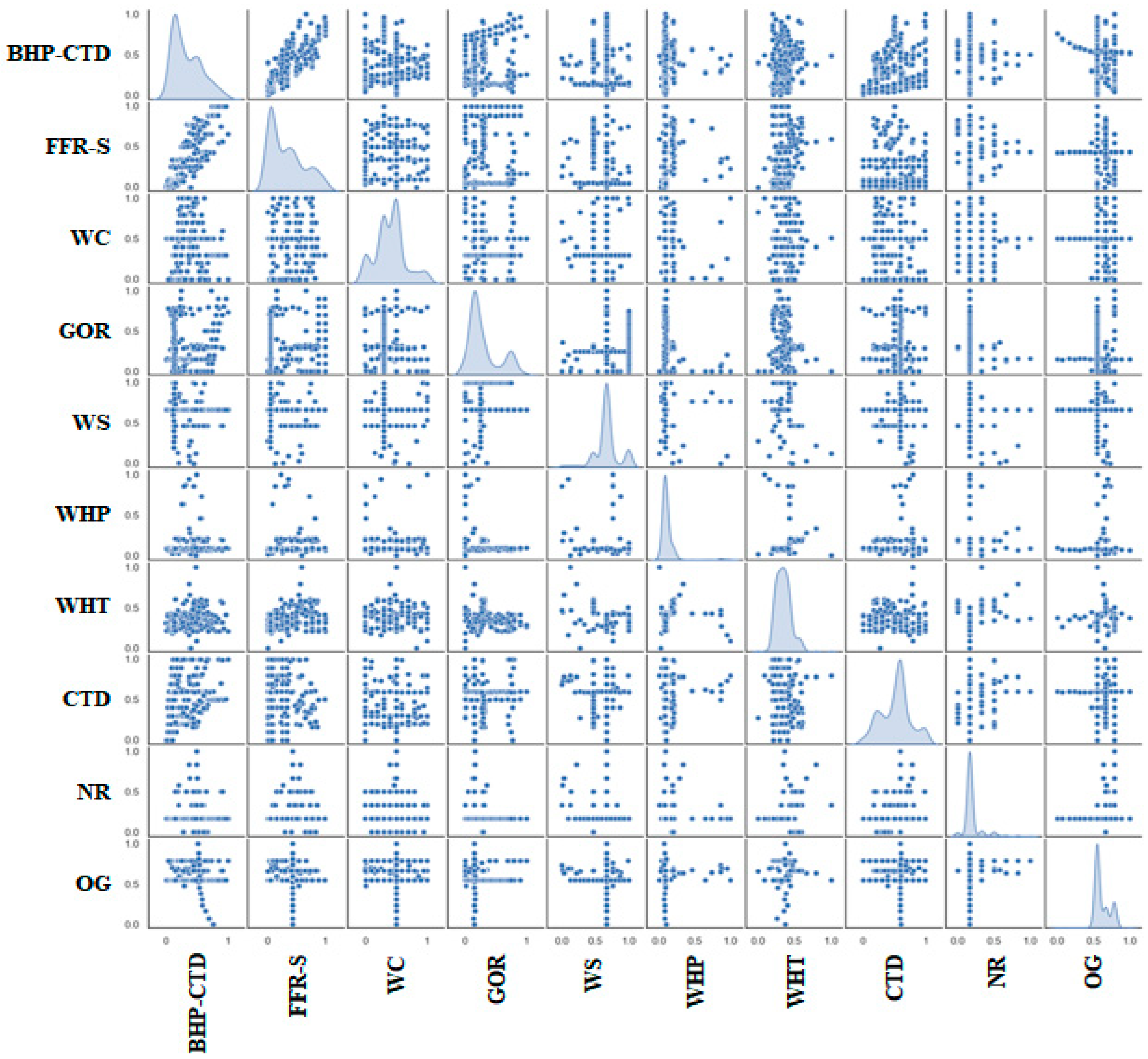
Figure 2 shows the pair plot of the correlations between the most important variables of the data set that will be employed to forecast BHP-CTD. The distribution of each variable is drawn on a diagonal, and correlations among bivariate variables are drawn on an off-diagonal. There is a certain amount of linear correlation between BHP-CTD and FFR-S and WC and CTD that suggests expected dependencies. Pair plots should be examined to see patterns of correlation and similarities in data, which are critical to enhance the model performance and to ensure that relevant and non-redundant input variables are used in ML models.
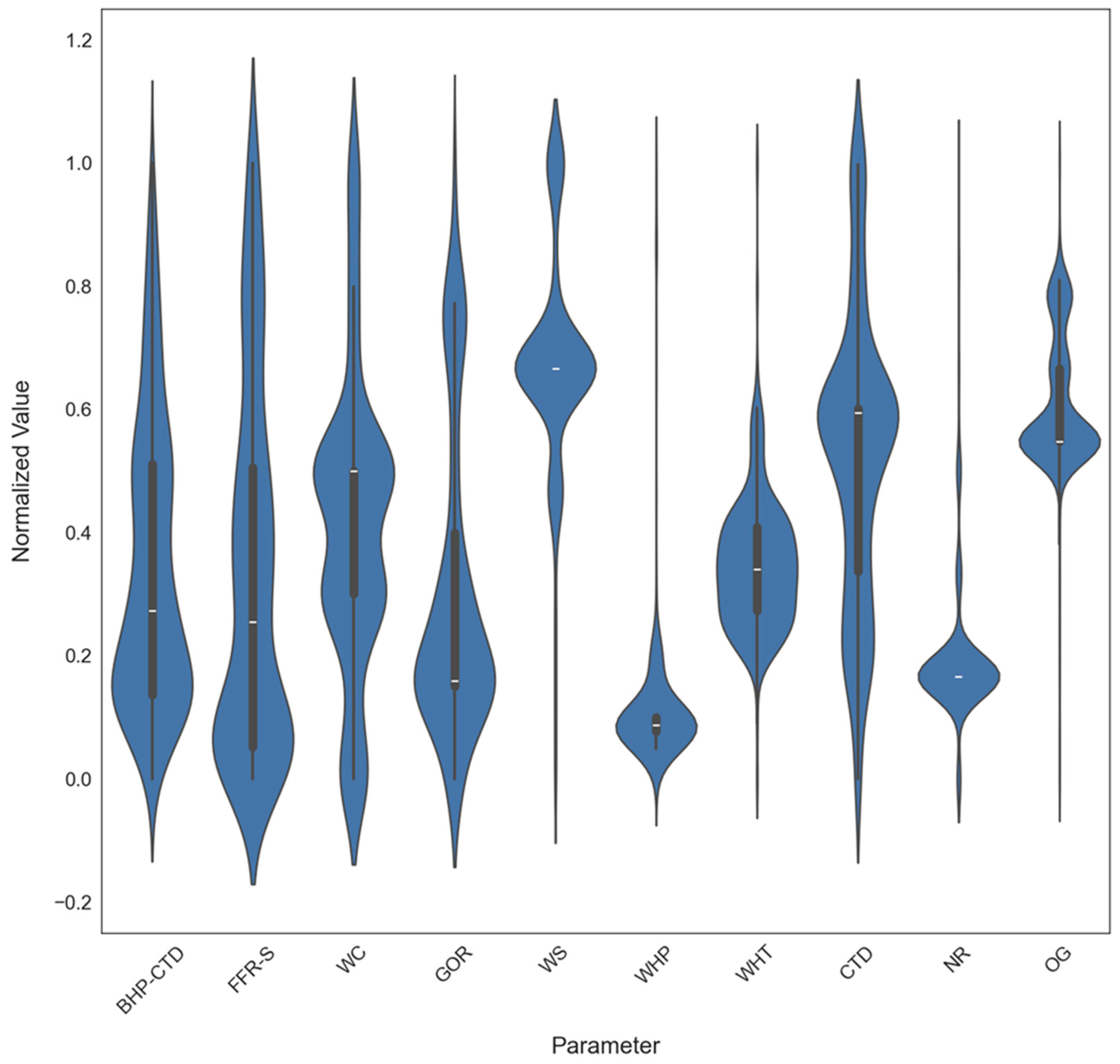
Figure 3 reveals the distribution of all the parameters employed in the estimation of BHP-CTD, via violin plots. Variables are represented on the x-axis, and normalized values, which are restricted within the range of 0 to 1, are represented on the y-axis. Each violin plot contains both the box plot and the kernel density estimate, which aid in providing a concise statistical overview and the distribution of the data. The median is indicated by the white line in the middle, and the black bar above it describes the middle 50 percent of the data (which is indicated by the IQR). The parts of a violin become broader when there are many values clumped together and narrower when there are fewer values clumped. The outliers are plotted as individual points, unlike the rest of the density estimation. Distributions are significantly different in all parameters. As an example, WS exhibits a symmetric distribution that is well defined around higher normalized values, which suggests that there is a consistent concentration among the samples. The distributions of WHP and NR are narrow with a low variability, indicating very stable measurements. FFR-S and CTD, in turn, are distributed more widely, which means that there are a lot of differences between samples. WC and GOR are multimodal, which suggests the existence of subgroups. The distribution of OG is a little skewed but narrow, the distribution of WHT shows a central maximum with some dispersion, and BHP-CTD is distributed moderately with symmetry.

2.2. Feature Ranking

The right understanding could be extracted out of the data fed to the ML algorithms. These ML models require strong and meaningful relationships between input parameters and the required parameter to obtain accurate performance. That is why the meaning of the features associated with the correlation coefficient must be understood. In the research, Pearson and Spearman were employed to calculate the correlation coefficient. The Pearson correlation coefficient (r) is utilized to show a linear correlation between two variables that are continuous but can easily be affected by outliers. Unlike Pearson, the Spearman rank correlation coefficient (ρ) is not very sensitive to outliers and can be used with non-normally distributed data that are monotonic only. The r of Pearson can only be applied in linear correlations, whereas Spearman’s ρ can identify any trend, though not necessarily in straight lines. The values of the two measures of correlation range between −1 and +1. When two variables have a +1 value, then when one variable increases, the other will increase. When the correlation is perfectly negative, −1 is a sign that the two variables will always move in opposite directions. The value of 0 implies that the variables are unrelated. Equations (1) and (2) characterize both measurements.
r = n X Y X Y n X 2 X 2 n Y 2 Y 2
where
n = number of paired observations
X , Y = data values
X Y = sum of the product of paired scores
X 2 , Y 2 = sum of squares
ρ = C o v R X , R Y σ R X σ R Y
where
R X , R Y = ranks of variables X and Y
C o v R X , R Y = covariance of the rank variables
σ R X , σ R Y = standard deviations of the rank variables
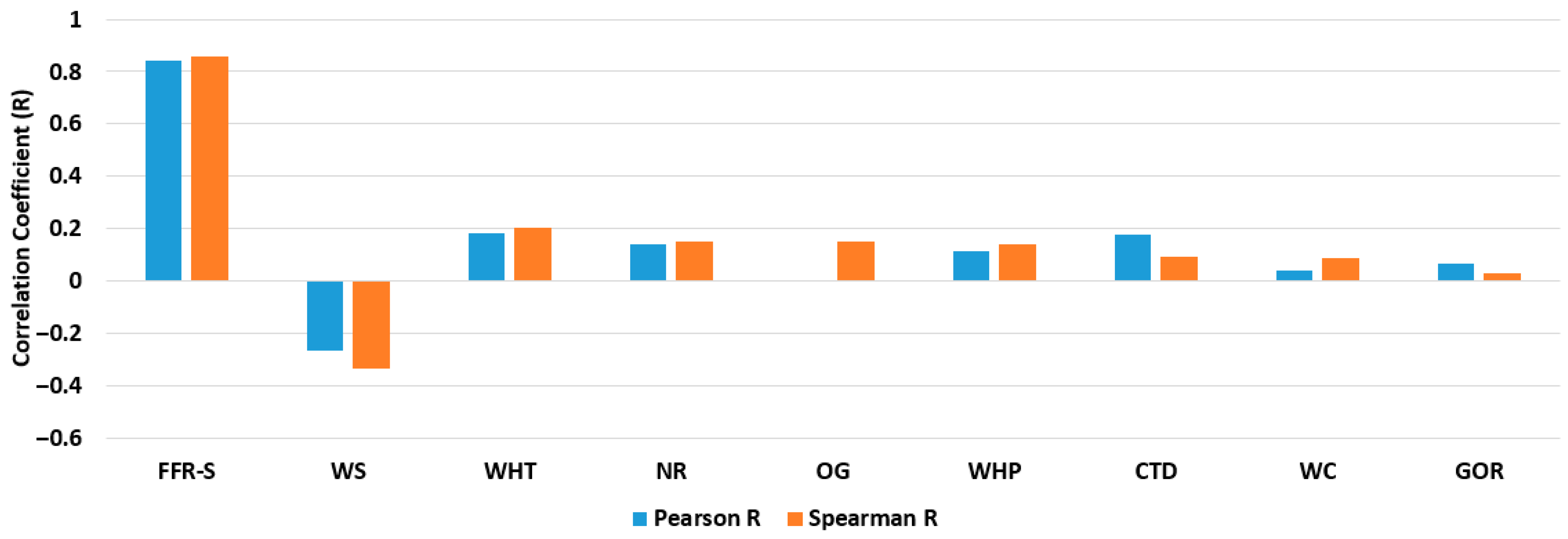
Figure 4 shows the magnitude of influence that input parameters FFR-S, WC, GOR, WS, WHP, WHT, CTD, NR, and OG have on BHP-CTD. BHP-CTD demonstrates a pronounced positive correlation with FFR-S, whereas its relationships with the other parameters are of medium strength.
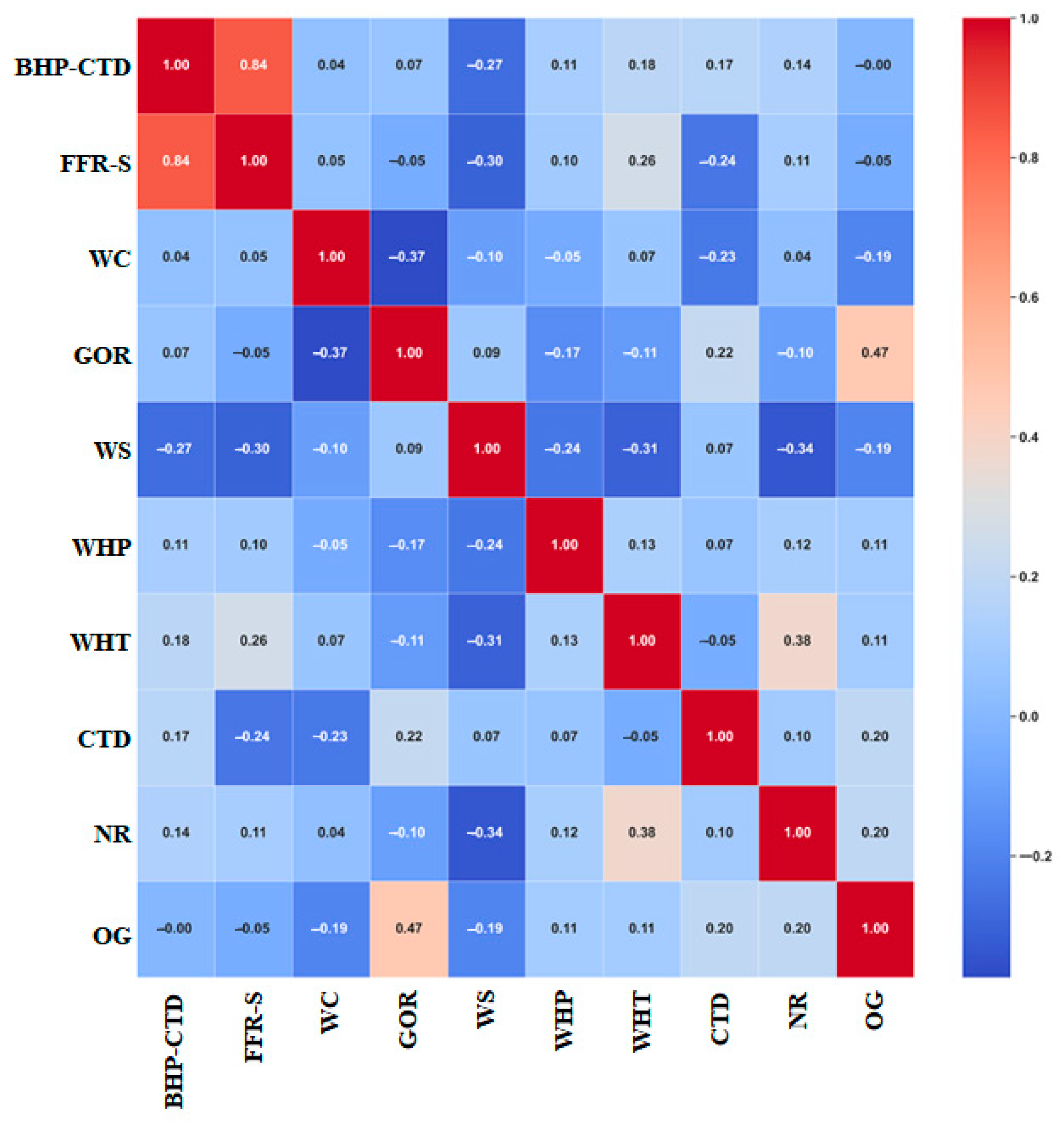
Figure 5 shows the heat map as a graphical representation of the correlation between all the parameters in the data set, based on the Pearson correlation matrix. The relationship between bottomhole pressure and the surface flow rate is large as indicated by the strongly positive correlation (0.84) between the BHP-CTD and FFR-S. The rest of the correlations are low or close to zero, like WC and WHP (−0.05), which means that there is no or a minimal linear relationship. In general, the heat map shows that the BHP-CTD and FFR-S are more connected, and such variables as WHP, WS, and WC seem to be more independent in the data. These observations provide, with huge significance, the parameters that affect nitrogen lifting operations and those that do not, which aids in explaining their behavior and forecasting their actions.
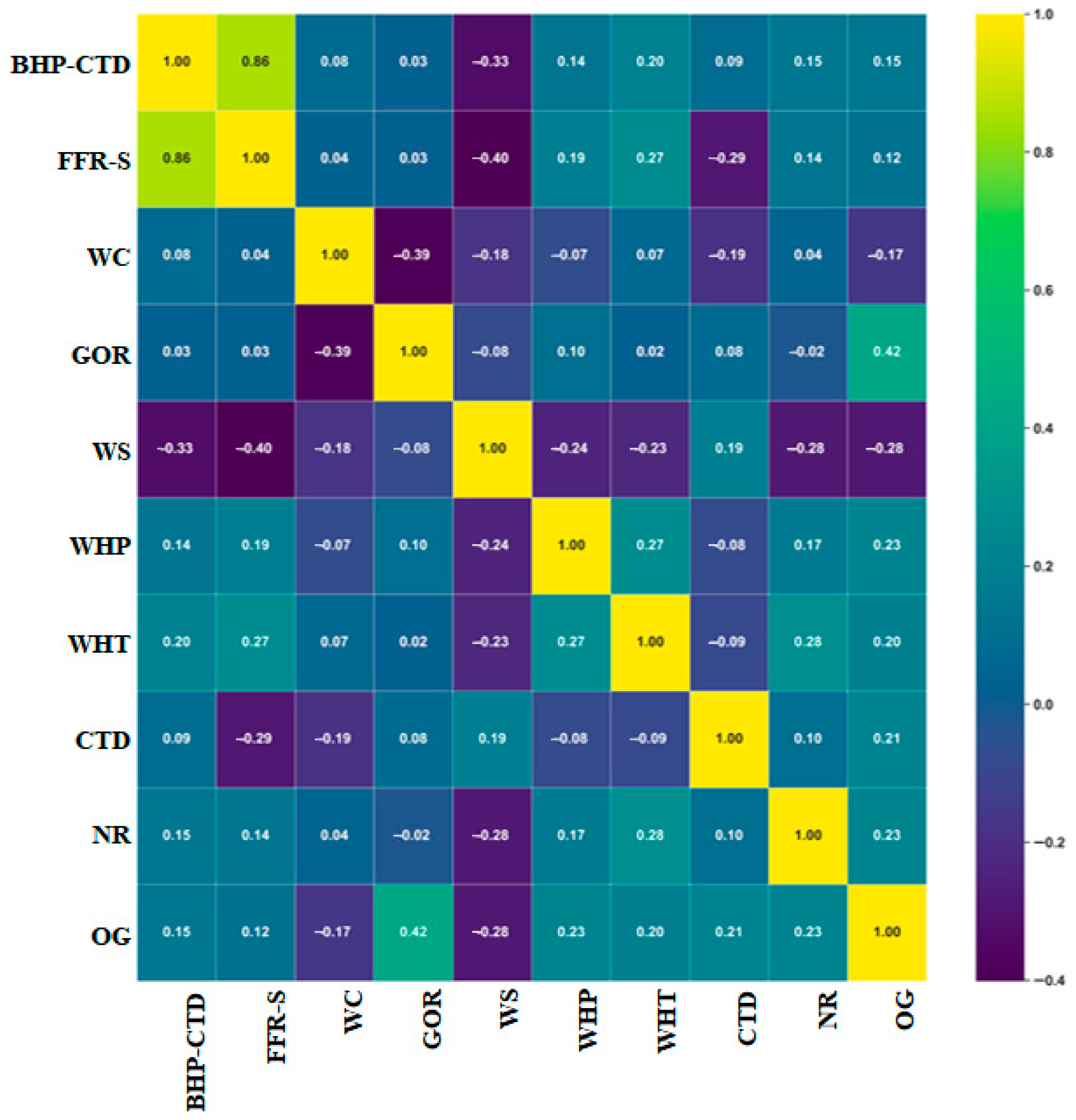
Figure 6 shows the Spearman correlation of all the features provided in the data to predict BHP-CTD in the form of a heatmap. It is observed that there is a strong positive correlation between BHP-CTD and FFR-S (0.86), indicating that the relationship is significant. In the meantime, other variables have low correlations with BHP-CTD.

2.3. Data Preprocessing

Machine learning preprocessing of data ensures that the data is consistent and suitable for the development of the model. The data processing includes procedures that authenticate the data as trustworthy, uniform, and precise, and this improves the quality and efficiency of the model. The initial step will include dealing with missing data. To handle missing values, it was decided to delete records with missing values. The use of box plots also helped us to detect and eliminate outliers because they may disrupt the process of learning. The removal of outliers incorporated the use of IQR-based detection and expert petroleum engineering review in order to maintain rare but valid operating conditions, therefore reducing the possibility of bias. Data integration is performed next, and it combines multiple data sources into a single set.
The last processing stage is standardization or normalization. When using regression machine learning models, normalization of data (i.e., adjusting numerical features to a common range) is used to avoid the fact that features with large magnitudes can dominate the learning process. This is essential when dealing with models that are sensitive to parameter scales, including gradient descent-based algorithms (e.g., neural networks, linear regression) and techniques based on distances (e.g., k-nearest neighbors, support vector machines). Some of the more popular ones are min-max scaling (scales the data to a specific range, usually [0, 1]) and standardization (scales the data so that it has a mean of zero and a variance of one). Min-max scaling has the benefit of having the same relationships as the original data points and is readily interpretable in the given range, which is why it is especially useful in cases where data is not distributed in a Gaussian manner or where upper and lower boundaries must be specified. Mathematically, min-max scaling can be written as
Y = X A B A
where
X is the original (raw) value,
A is the minimum value in the dataset,
B is the maximum value in the dataset,
Y is the normalized value after scaling to the range [0, 1].
Finally, the data that was processed was divided into 80 percent, which was used in training, and 20 percent, which was used in testing. We select this number to assist in making sure that the model has sufficient data to learn and sufficient unseen data in order to evaluate its capacity to address any new problem and observe overfitting.

2.4. Models Structure

2.4.1. Conventional Predictive Models

Fifteen traditional models were established and examined on Python 3.10.12, and each model demanded the hyperparameter configurations outlined in Table 2. In this study, several regression-based algorithms are utilized, such as Neural Network (L-BFGS), AdaBoost, Extreme Gradient Boosting (XGBoost 3.0.4), Gradient Boosting via Scikit-Learn, distance-weighted k-Nearest Neighbors, CatBoost 1.2.8, Stochastic Gradient Descent (used here under the form of the scikit-learn SGDRegressor 1.7.1 of linear regression with Elastic Net regularization), Support Vector Machines, Random Forests, and uniform kNN, since relying on just one predictive model is insufficient due to the diverse nature of the dataset. Different models have different underlying assumptions and learning mechanisms and inductive biases, and so some architectures are better suited to particular data distributions, complexities, or noise levels. As an example, LR is applied because of its simplicity and interpretability, DT is chosen because of its power to derive understandable decision rules, RF is chosen because of its robustness and its ability to evaluate feature importance, and kNN is used to learn non-parametric, local relationships in the data. The sequential boosting approach (such as ADAB) improves poor learners, whereas gradient boosting and especially XGBoost are high-performance, efficient, and have excellent capabilities of working with complex data and missing values; CatBoost is especially good with categorical features. SVMs work well in high-dimensional areas where there is a definite margin. When handling large datasets, SGD is efficient. Lastly, NN is strong in the application to highly non-linear patterns and complex interactions, with various optimizers affecting convergence. On the activation functions, we tried ReLU, tanh, sigmoid, and Swish; ReLU produced the best accuracy and stability. The NN architecture used in this study had a single hidden layer that contained 50 neurons that used an activation function of ReLU. This structure was chosen because of the initial testing that demonstrated that it offers a good trade-off between accuracy and computational efficiency and a low chance of overfitting. The weight initialization scheme was according to the Xavier/Glorot scheme in scikit-learn, and this resulted in stable convergence. Even though we have considered deeper or alternative architectures, we were interested in benchmarking various algorithms as opposed to performing a comprehensive NN architecture search. While Adam and SGD are widely adopted and robust in many applications, in our dataset L-BFGS provided superior accuracy with minimal tuning. Such a comparative approach is what will help us to choose a model that is most appropriate to the specificities of our dataset so that we will have the highest accuracy of predictions and generalization.
Model hyperparameters specify the behavior and the operations of machine learning models. Regression machine learning model hyperparameters are external configuration options that are specified manually prior to the training process and not learned by the data. They are vital since they determine the manner in which the model learns as well as its general structure and have a tremendous impact on its performance and capacity to generalize to unseen data. As an example, we constrained Random Forest to 10 trees in our setup after initial tuning revealed that any more trees would not improve its accuracy significantly, but with Gradient Boosting we needed 100 consecutive trees to reach a converged result. Such a difference is not a contradiction but an inbuilt learning dynamic of the two algorithms. As an example, on tree-based models, the number of trees influences the complexity and robustness of the model, and the maximum depth of the tree determines the maximum depth that the individual trees can extend and therefore directly influences the risk of overfitting. The iterative optimization algorithms have a learning rate that controls the step size to the optimal solution, which impacts the speed and accuracy of convergence. The strength of the regularization is critical in the prevention of overfitting, which penalizes complex solutions, favoring simple solutions. The iteration limit is the upper bound of the training cycles, which balances the model fit and the cost of computation. It is important to tune these hyperparameters properly in order to produce the optimal bias and variance trade-off, producing robust performance and good generalization. All models used a controlled tuning procedure: grid search in low-dimensional spaces (e.g., decision trees) and random search with subsequent fine-tuning in high-dimensional spaces (e.g., neural networks, boosting techniques). Literature ranges, domain expertise, and 10-fold cross-validation performance were used to guide the selection to achieve accuracy, stability, and computational efficiency.
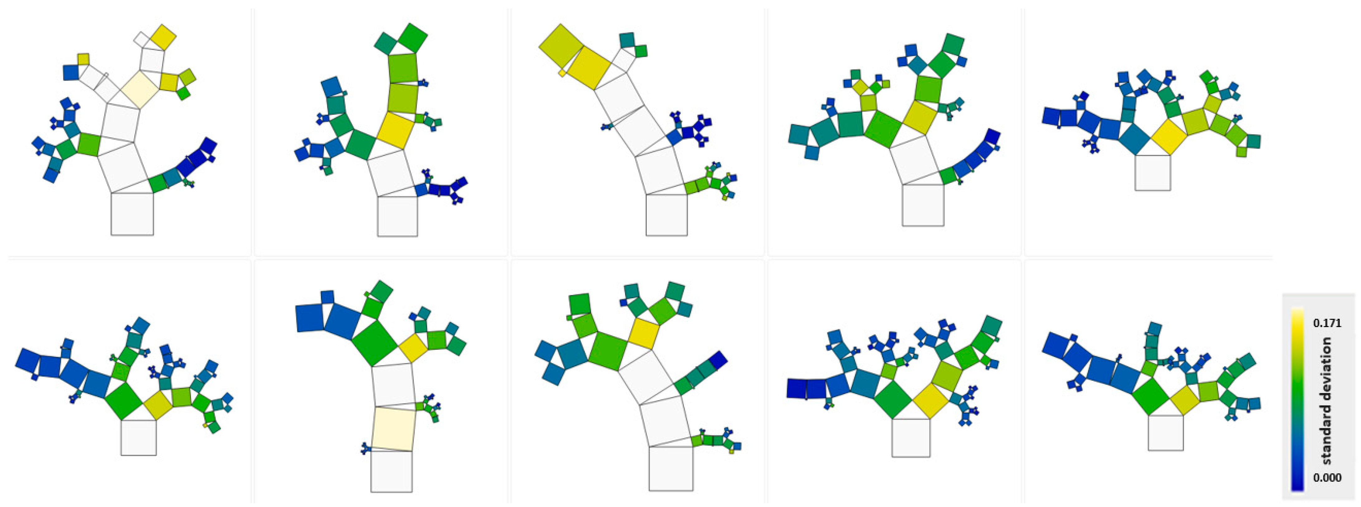
Figure 7 shows Pythagorean Forest conception of the RF algorithm that displays all single decision trees generated by the model. The shortest branches in this kind of visual are the most desirable ones because they have darker colors and indicate fewer but more significant splits that are effective to divide the data. The visualization is very useful to understand the underlying structure and diversity of the constituent trees of the ensemble. This will also enable us to tell the contribution of each tree to the final prediction and also give us possible signs of either model over-specialization or insufficient learning, like the repetition of branching patterns or over depth in the forest.

2.4.2. Genetic Programming-Based Symbolic Regression

The sixteenth model employs Symbolic Regression through Genetic Programming (GPSR). The GPSR implementation was developed using Python version 3.10.12 via the PySR library, and the detailed hyperparameters used for this model are listed in Table 3. The machine learning method GPSR is an evolutionary algorithm that automatically discovers a mathematical formula that fits a dataset best. In contrast to classical regression models, in which parameters are optimized in a fixed structure, GPSR searches over a vast search space of potential mathematical expressions in the form of “trees” of operations and variables. It develops a population of such expressions across generations by applying genetic operators such as mutation and crossover, and a fitness function determines which of the most fitting formulas are used.
The key benefit of the GPSR against the traditional regression models is that it can find new, interpretable mathematical equations without prior assumptions on the nature of the relationship. Although numerous classical models, including neural networks, tend to act as black boxes, which offer precise predictions, GPSR produces human-readable formulas. Such readability is amazingly useful in complex processes such as nitrogen lifting, where knowledge of the underlying laws or relationships is as important as predictive precision. Also, GPSR is capable of naturally accomplishing feature selection and highly generalized models by finding the simplest mathematical form that describes the data well.

3. Results and Discussion

3.1. Model Results

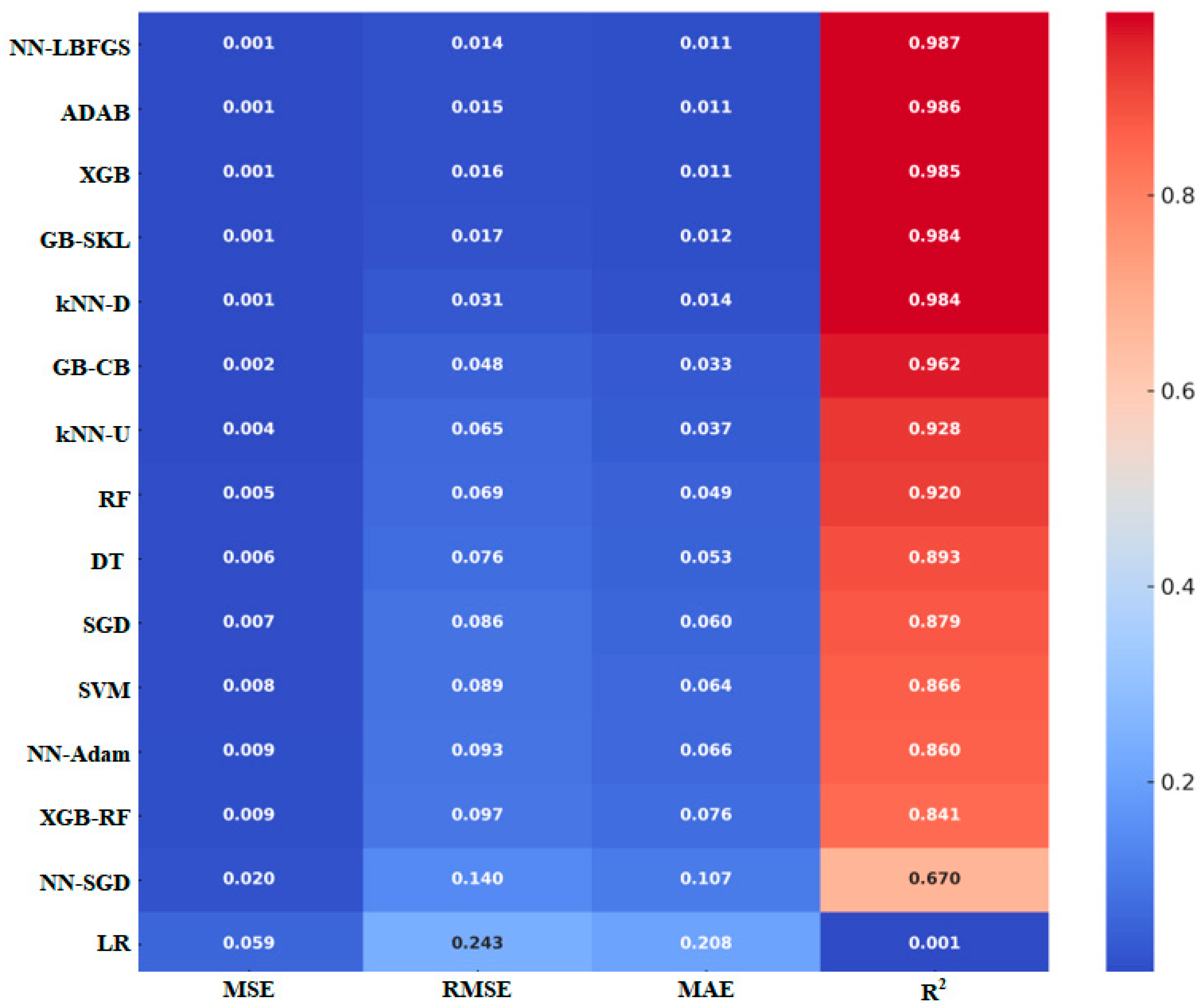
Figure 8 shows the accuracy of the machine learning models based on mean square error (MSE), root mean square error (RMSE), mean absolute error (MAE), and coefficient of determination (R2). The accuracy of each model is determined based on the computed results. Models with low error values and high R2 scores demonstrate strong predictive ability, whereas high errors combined with low R2 values reflect weaker performance. It is important to point out that these values of errors are calculated on normalized data (scaled to [0, 1]), this is why the rather small values are observed. Among the models tested, the NN (L-BFGS) achieves the highest performance.
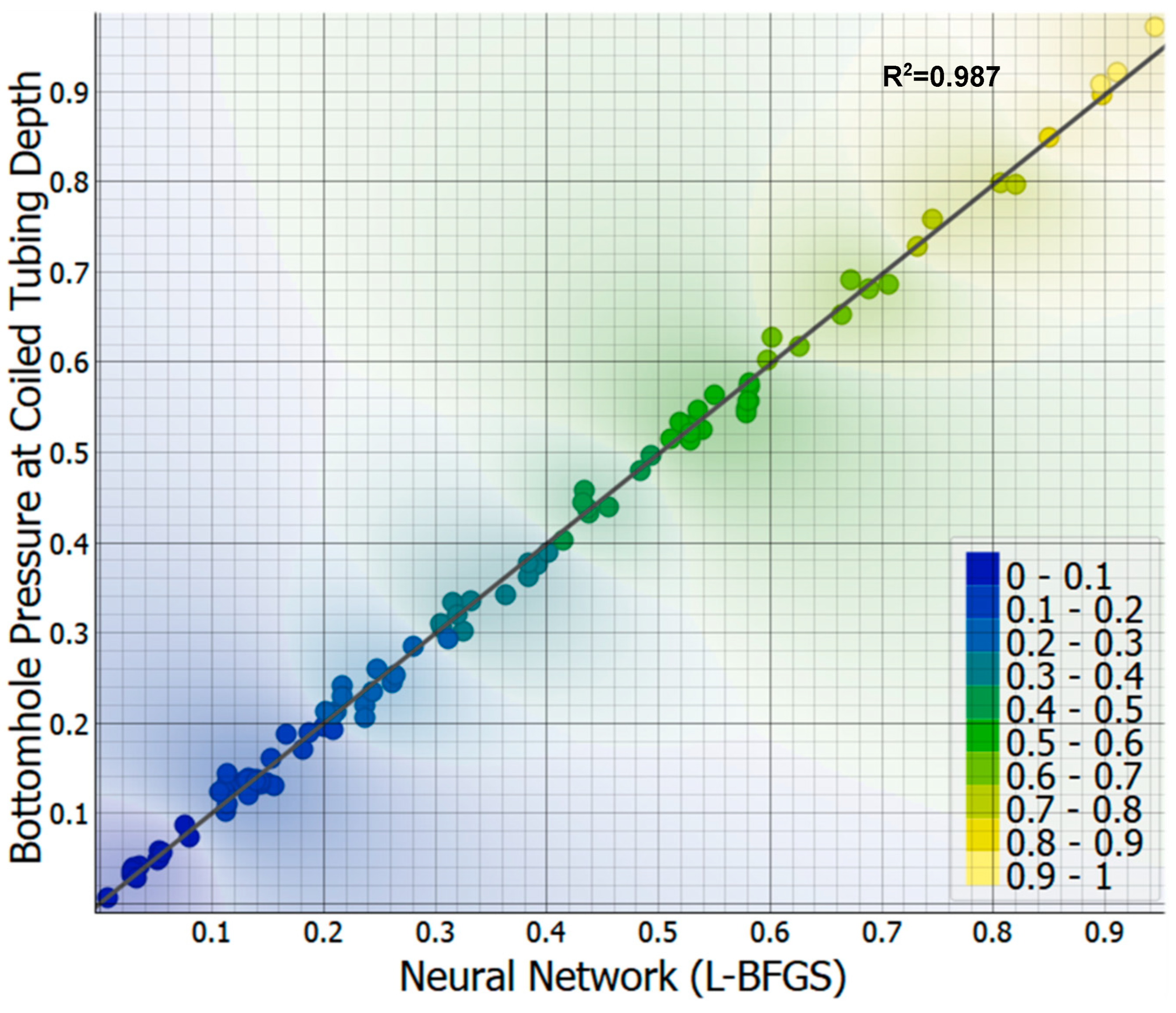
The observed values of the downhole pressure gauges and the predicted values of the BHP-CTD according to the NN (L-BFGS) model are displayed in Figure 9. The clustering of data points at the diagonal line shows the great accuracy of the model predictions. The smooth blue-yellow gradient is further evidence that the model is consistent at all the pressure range. The small spread about the diagonal shows that there is little deviation in real measurements and the similarity of the color distribution certifies the validity and applicability of the model under different pressures.
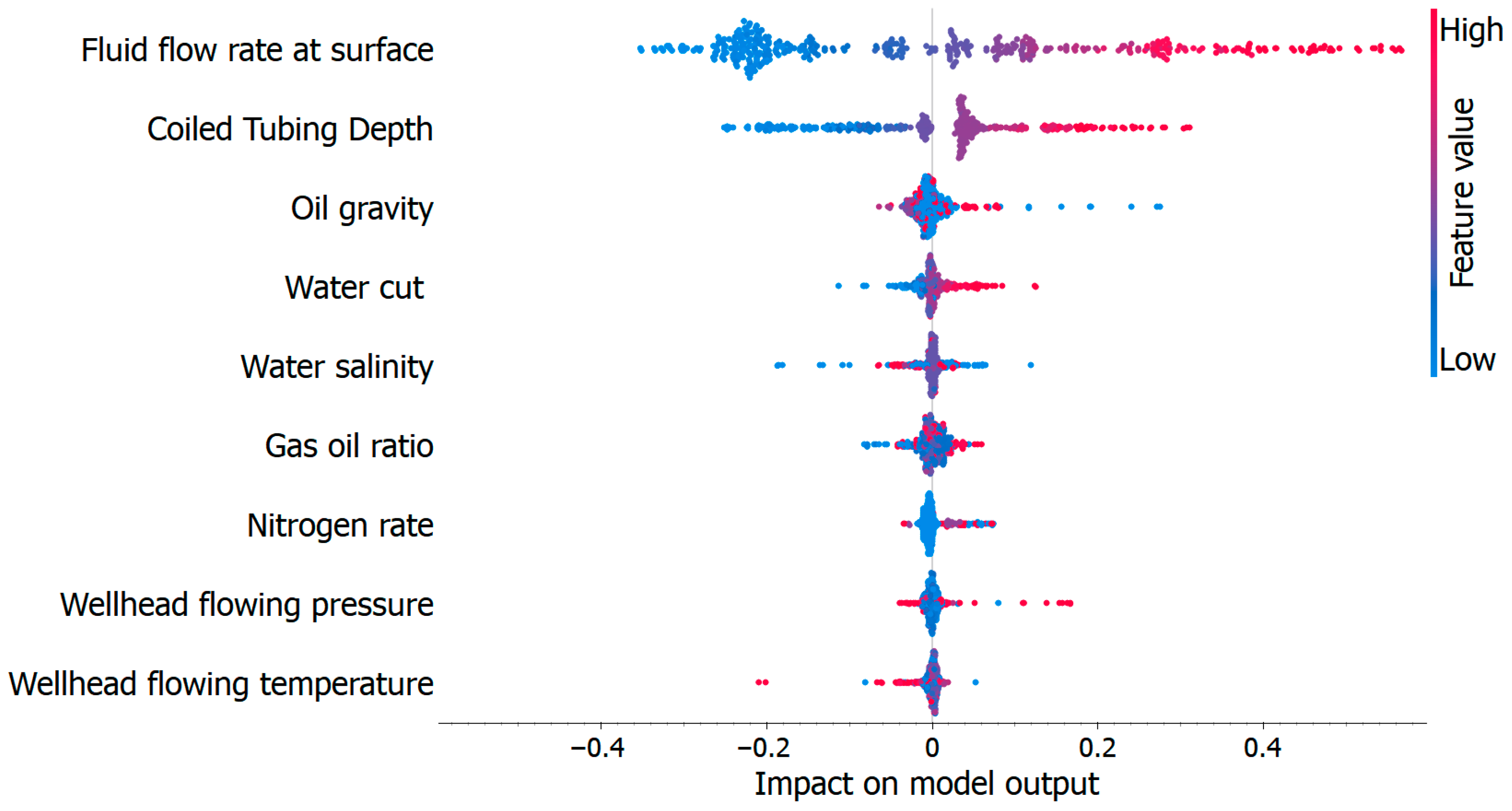
In Figure 10, the primary variables that affect the BHP-CTD prediction based on the NN (L-BFGS) model using SHAP (SHapley Additive exPlanations) are reported. The SHAP values explain how each feature is influencing the outcome of the model in order to explain the behavior of the model. SHAP values, or the effects of each input (positive or negative), are located in the horizontal axis. Each observation is highlighted with a point that is determined by the values of the feature (blue is the lowest and red is the highest), and its location is determined by the corresponding SHAP value.
All the parameters are ranked from most important to least important, with the most important at the top. FFR-S and CTD seem to play the biggest role in the variation in the BHP-CTD prediction, as they demonstrate the widest range of SHAP values up and down. SHAP presented different results when compared to Spearman and Pearson because it aims at giving the significance of features in a particular model, whereas the two methods only look at the regions where one feature has an influence on another in a linear or single-directional manner. Thus, SHAP finds more complex relationships and their meaning as opposed to simple correlation statistics. SHAP values can assist domain experts to understand the same results, understand how the model makes judgments, identify important factors in the domain, and examine the real meaning of the parameters used in the study. Both NN-LBFGS and symbolic regression are also lightweight in terms of computational cost: a neural network only takes 3–5 ms to make a prediction, whereas symbolic regression takes <1 ms to evaluate. Such latencies are insignificant in comparison to the SCADA system refresh rates, which proves their ability to be applied in real time.
In GP-SR, normalized data were used to form interpretable models. After testing, the selected model (Equation (4)) had a high performance with MSE of 0.004, RMSE of 0.063, MAE of 0.038 and R2 of 0.94. Equation (4) provided the best trade-off between predictive accuracy and structural simplicity of the symbolic models in Table 4. It had the least loss of 0.00303 at a complexity of 17. The complexity of a model is determined by the variables and operations that it uses and consequently affects interpretability. Given that the lesser the value of error, the better the fit, Equation (4) is the most appropriate model since it is a balance between accuracy and relative simplicity. Interestingly, the FFR-S and CTD dependence is in line with mechanistic multiphase flow formulations where the velocity and hydrostatic head are determinants of pressure gradients. The nonlinear terms added are not interpretable but act as convenient proxies to complex slip and holdup effects that are usually encapsulated in mechanistic models by empirical closure relations.
c o s ( W S ) C T D ( ( ( W C + G O R ) + C T D ) W S ) + F F R _ S F F R _ S

3.2. Model Testing and Validation

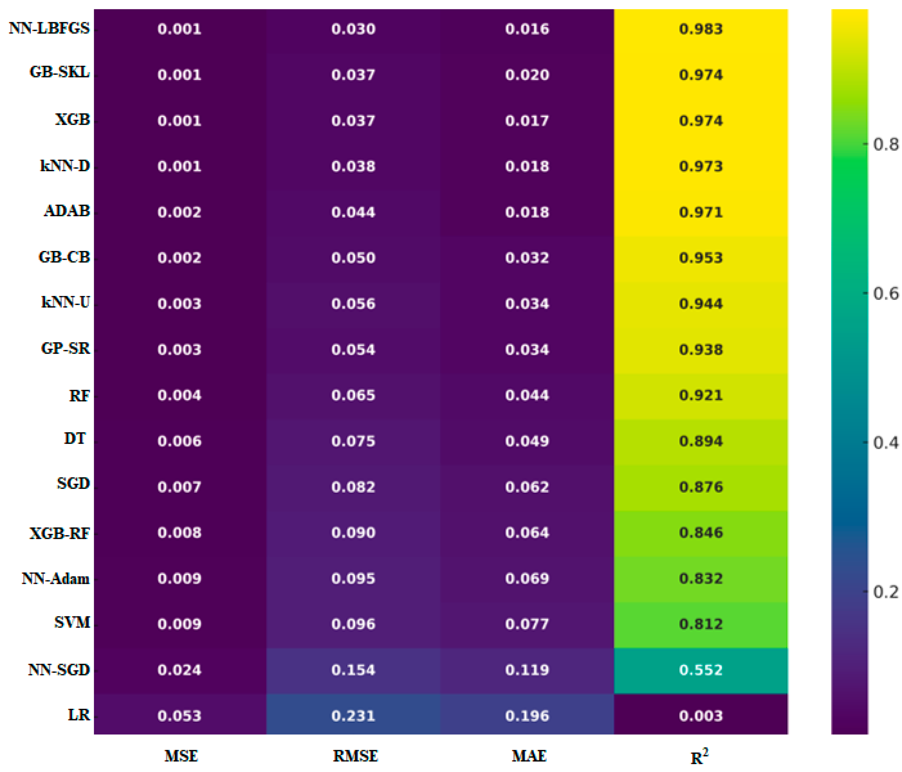
In order to identify the performance of the ML models developed, k-fold cross-validation tests are conducted, as well as random sampling methods. The approaches discussed here provide a collection of steps to be used to test the models and enable professionals to concur on their effectiveness. In machine learning, K-fold cross-validation performs a K-fold partition of the data, and only one of the folds is tested, the rest being part of the training. It is performed K times, and the accuracy measures of prediction are averaged after each iteration. The method is useful in constructing models as it provides a more reliable estimation of the way the model will perform with new data. It avoids overly positive evaluation of an algorithm by training and validating it on all the available data. It is also critical in selecting the most appropriate hyperparameters, the selection of the model to use, and the reduction in certain forms of bias. In the cross-validation, there is training on nine folds and testing the regression model with the only left fold (it is a test set). The result of the 10-fold cross-validation is shown in Figure 11. The outputs indicate the MSE, RMSE, MAE, and R2 by each model.
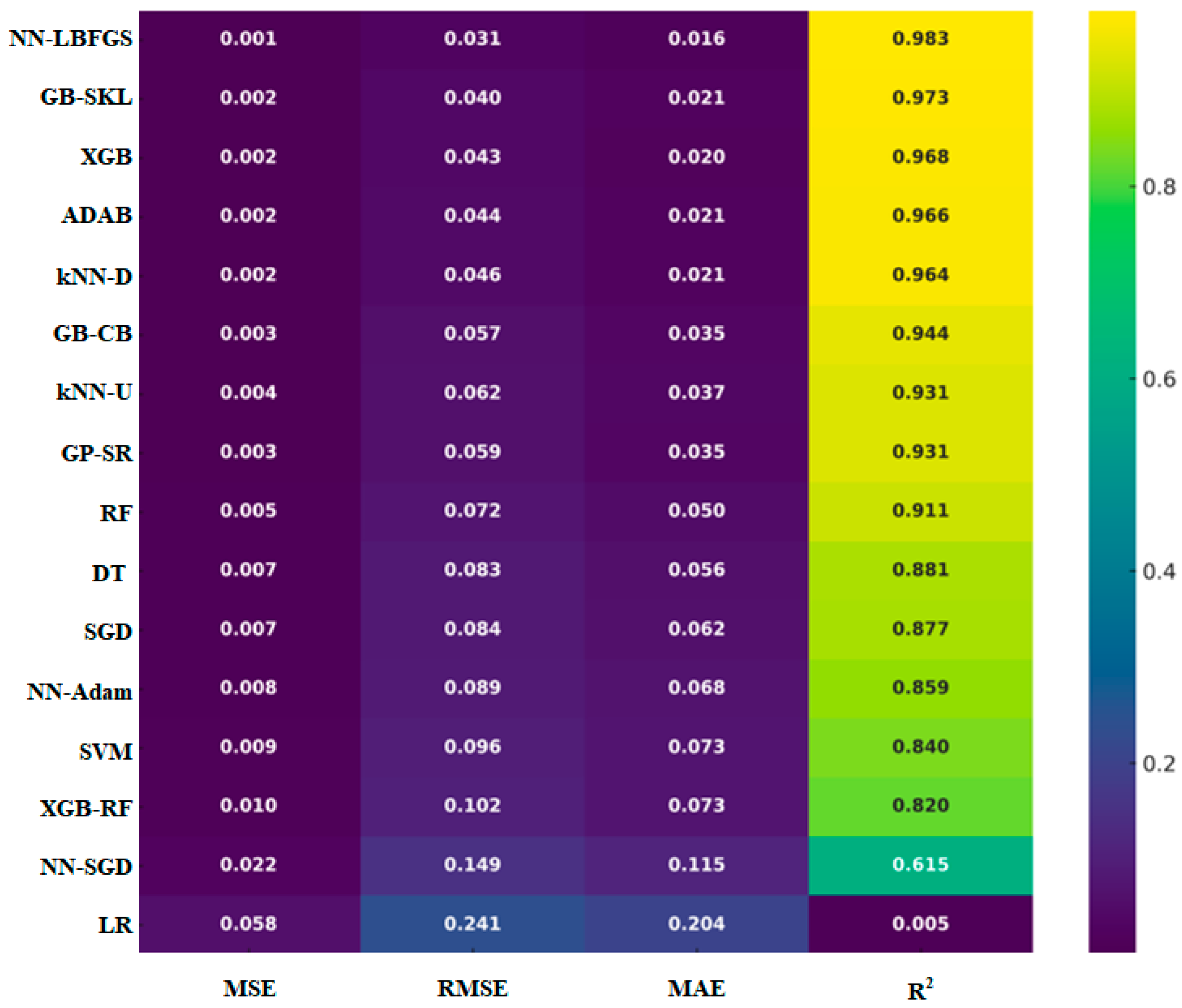
In repeated random sampling cross-validation (RRSCV), the data is randomly divided into training and test parts several times. Contrary to the fixed splits involved in K-fold cross-validation, RRSCV involves multiple random splits in order to minimize the variability of its performance estimates. The primary advantage is that this approach is more efficient in using the small data, and the findings are more confident in terms of how the model would perform with new data. It can also be used to determine whether a model is overfitting, and it can be used to tune hyperparameters effectively, which can be used to choose the most appropriate model in cases where data is ambiguous. The result shown in Figure 12 was obtained using the RRSCV technique after 10 iterations were performed. Each of the models is provided with its MSE, RMSE, MAE, and R2. During K-fold and RRSCV assessment, the neural network (L-BFGS) model is awarded a superior accuracy compared to the other models.

3.3. Field Application

The next validation process to be discussed is blind dataset validation. By validating your dataset blindly, you can have an estimate of the accuracy of your model in the real world because you did not train, tune, or select the features on the new dataset. This form of validation isolates the test in advance; thus, the possibility of data leakage when developing a model is eradicated. The 29 blind-validation wells were geographically and operationally different than the training set and represented different formations and operating conditions in order to provide the best assessment of true generalizability. Although consistency can be enhanced with the help of K-fold and bias can be minimized through sampling the data multiple times, blind validation is the most accurate and pure review. As such, the most accurate algorithm (developed NN (L-BFGS) model) was used with independent data of 29 vertical oil wells to predict the BHP-CTD during nitrogen lifting operations. Table 5 is used to gather descriptive statistics of each parameter.
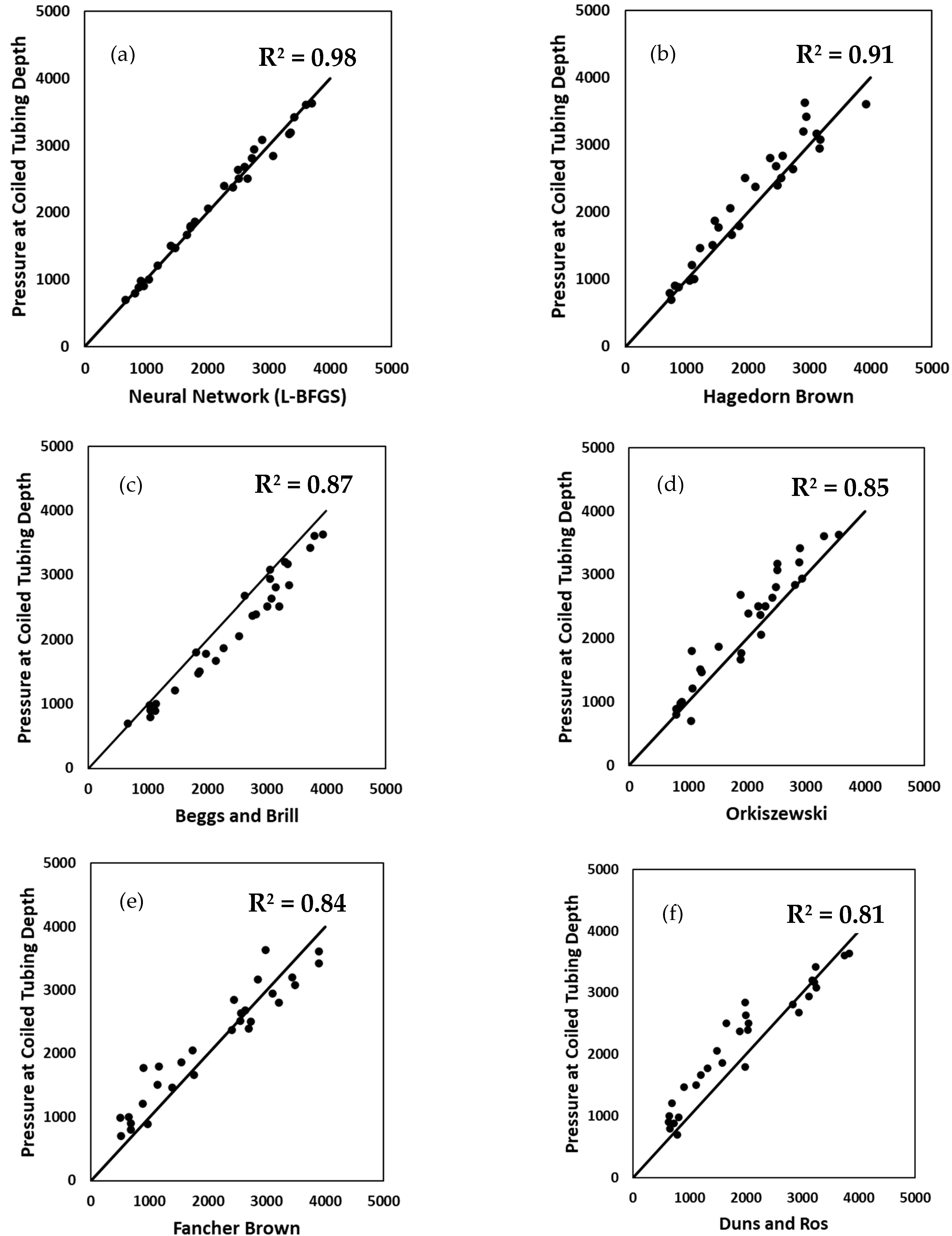
Figure 13 illustrates a comparative study of the bottomhole pressure values calculated with the developed neural network model using the L-BFGS optimization algorithm with the bottomhole pressure estimates based on the conventional vertical lift correlations, such as Hagedorn and Brown, Fancher and Brown, Beggs and Brill, Orkiszewski, and Duns and Ros, and compared to the actual bottomhole pressure gauge data. Moreover, Table 6 shows the results of the different BHP-CTD prediction techniques, such as a neural network and five correlations. Evaluation metrics, MSE, RMSE, MAE, and R2 all indicate that the neural network gives the most accurate predictions and Duns and Ros the least accurate of all the methods tested. The use of the neural network (L-BFGS) algorithm on the data of 29 wells shows that it is much better at predicting BHP-CTD as opposed to the traditional empirical correlations. This model allows continuous monitoring and optimization of nitrogen lift operations. Moreover, it presents a cheap and dependable substitute for bottomhole pressure gauges. Such machine learning models, in contrast to more conventional physics-based, empirical, or unified models, are less prone to calibration issues and performance decline with time. In the current research, the NN-LBFGS model was used as post hoc to benchmark its accuracy. Nevertheless, it is in a lightweight form that can be easily put in real-time use through incorporation with SCADA systems, as all the necessary inputs are regularly obtained by field sensors.
The ML models were more accurate, flexible, and real-time applicable compared to empirical correlations like Hagedorn and Brown, Beggs and Brill, and Orkiszewski. In order to make a clearer overview of these benefits, Table 7 was also included to compare the relative strengths and limitations of the machine learning models applied to this study with those of traditional empirical and mechanistic approaches. This comparative viewpoint lays stress not only on the better predictive accuracy of data-driven methods but also on their exclusive capacity to adjust to various working circumstances, lower the dependency on expensive gauges, and allow online monitoring.

3.4. Drawbacks of Machine Learning Techniques in BHP-CTD Forecasting

While highly accurate in forecasting BHP-CTD during nitrogen lifting, these ML models also present some constraints. They depend on large and properly prepared data and may not operate well with wrong, inadequate, or biased data. From a practical standpoint, implementation may also face challenges such as integration into existing operational workflows, underscoring the importance of gradual deployment strategies. They are not easily interpretable, as is the case with physics-based models; hence, the reasoning behind their actions is not clear. Frequent retraining might be needed when there are changes in operational settings or well configurations. Practically, we suggest retraining the models every 12 months or earlier in case substantial new well data are obtained in order to guarantee robustness and versatility.
The model performance can be hyperparameter sensitive and data preprocessing sensitive. In addition, these models might not be able to model complex nonlinear relationships when the architecture is not sophisticated. The other issue is the overfitting, particularly when the data is high-dimensional. The model selection is a limitation in itself, and, as argued in the Future Work section, a further step is the investigation of more advanced architectures. Lastly, the models are dependent on certain inputs (coiled tubing depth and nitrogen rate), but fallback plans (limited-input retraining using leading predictors (e.g., FFR-S and CTD) or statistical imputation) can overcome missing data problems so that the models are operational.

4. Conclusions and Future Work

A critical comparison of 16 machine learning regression models was carried out to estimate flowing bottomhole pressure at coiled tubing depth (BHP-CTD) during nitrogen lifting, drawing on a comprehensive dataset from 518 vertical wells. The L-BFGS-based neural network showed the best predictive accuracy in all the cases, with an R2 of 0.987 and error metrics being minimal in the k-fold, random sampling, and blind validation tests. This superior performance, especially in comparison to the traditional empirical correlations (e.g., Hagedorn and Brown, Beggs and Brill), highlights the great benefit of data-driven methods in the modeling of the nonlinear, complex relationships involved in multiphase flow in dynamic wellbore conditions. An additional advantage is that the interpretable derivation of a symbolic regression model with an R2 of 0.94 offers a transparent counterpart, filling the gap between predictive strength and physical understanding. The findings can be used to improve the existing practice by providing a reliable, cost-effective, and real-time alternative to the conventional methods and costly downhole pressure gauges and, in this way, help optimize the parameters of nitrogen lifting more precisely and make timely and informed decisions on the possible necessity of artificial lift systems or stimulation operations.
Further research is necessary to make these models more robust and broadly applicable by using a broader range of field data that cover the variety of reservoir types, coiled tubing specifications, operational conditions, wellbore geometries, and fluid properties. Combining time-series data and dynamic operational parameters will play a key role in the development of genuinely adaptive models with the ability to optimize performance in real-time in transient conditions. Investigation of physics-informed machine learning, and especially its combination with symbolic regression, looks like a promising direction to obtain models that are not only very accurate but also physically consistent and interpretable. Finally, the ongoing creation of intuitive software tools to train, deploy, and monitor models continuously, as well as a collective push to collect global field data, will accelerate the rate of adoption of these sophisticated predictive tools, which will fundamentally change optimization approaches to complex nitrogen lift operations, particularly in mature fields with large well networks.

Author Contributions

Conceptualization, S.N.; methodology, R.M.; validation, S.N.; formal analysis, S.N.; investigation, S.N.; resources, R.M.; data curation, R.M.; writing—original draft preparation, S.N.; writing—review and editing, R.M.; visualization, S.N.; supervision, R.M.; project administration, R.M. All authors have read and agreed to the published version of the manuscript.

Funding

This research received no external funding.

Data Availability Statement

The original contributions presented in the study are included in the article, further inquiries can be directed to the corresponding authors.

Conflicts of Interest

The original contributions presented in the study are included in the article, further inquiries can be directed to the corresponding authors.

Nomenclature

AdaBoostAdaptive Boosting
AdamAdaptive Moment Estimation optimization algorithm
BHPBottomhole pressure
BHP-CTBottomhole Pressure at Coiled Tubing Depth
CTDCoiled Tubing Depth
DTDecision Trees
FFR-SFluid flow rate at surface
GB-CBGradient Boosting (catboost)
GB-SKLGradient Boosting (scikit-learn)
GORGas–oil ratio
GP-SRGenetic Programming-based Symbolic Regression
IQRInterquartile range
kNN-DK-Nearest Neighbor (By Distances)
kNN-UK-Nearest Neighbor (Uniform)
L-BFGSLimited-memory-Broyden-Fletcher-Goldfarb-Shanno optimization algorithm
LRLinear Regression
MAEMean absolute error
MAPEMean absolute percent error
MLMachine learning
MSEMean square error
NNNeural Network
NRNitrogen rate
OGOil gravity
rPearson’s correlation coefficient
R2Correlation coefficients
RFRandom Forest
RMSERoot mean square error
RRSCVRepeated random sampling cross-validation
SGDStochastic Gradient Descent
SHAPSHapley Additive exPlanations
SVMsSupport Vector Machines
WCWater cut
WHPWellhead pressure
WHTWellhead temperature
WSWater salinity
XGBExtreme Gradient Boosting (xgboost)
XGB-RFExtreme Gradient Boosting Random Forest (xgboost)
ρSpearman’s rank correlation coefficient

References

  1. Hashmi, U.I.; Osisanya, S.; Rahman, M.; Ghosh, B.; Subaihi, M.H.; Kuwair, H.F.B.; Fathy, A.; Afagwu, C.; Mahmoud, M. Optimization of Nitrogen Lifting Operation in Horizontal Wells of Carbonate Formation. In International Petroleum Technology Conference; IPTC: Riyadh, Saudi Arabia, 2022. [Google Scholar] [CrossRef]
  2. Aitken, B.; Livescu, S.; Craig, S. Coiled Tubing Software Models and Field Applications–A Review. J. Pet. Sci. Eng. 2019, 182, 106308. [Google Scholar] [CrossRef]
  3. Han, G.; Ma, G.; Gao, Y.; Zhang, H.; Ling, K. A New Transient Model to Simulate and Optimize Liquid Unloading with Coiled Tubing Conveyed Gas Lift. J. Pet. Sci. Eng. 2021, 200, 108394. [Google Scholar] [CrossRef]
  4. Gao, K.; Zhao, Q.; Zhang, X.; Shang, S.; Guan, L.; Li, J.; Xu, N.; Cao, D.; Tao, L.; Yuan, H.; et al. Temperature Field Study of Offshore Heavy Oil Wellbore with Coiled Tubing Gas Lift-Assisted Lifting. Geofluids 2023, 2023, 8936092. [Google Scholar] [CrossRef]
  5. Zand, N.; Arjmand, Y.; Motamedikia, M.; Pourbahador, M. Economic Equation and Optimization of Artificial Gas Lift with Coil Tubing Based on Dynamic Simulation in One of Iranian Offshore Fields. IJNC 2020, 8, 111–130. [Google Scholar] [CrossRef]
  6. Michel, G.; Civan, F. Modeling Rapid Multiphase Flow in Wells and Pipelines Under Nonequilibrium and Nonisothermal Conditions. In Proceedings of the Rocky Mountain Oil & Gas Technology Symposium, Denver, CO, USA, 16–18 April 2007; SPE: Richardson, TX, USA, 2007. [Google Scholar] [CrossRef]
  7. Yudin, E.; Khabibullin, R.; Smirnov, N.; Vodopyan, A.; Goridko, K.; Chigarev, G.; Zamakhov, S. New Applications of Transient Multiphase Flow Models in Wells and Pipelines for Production Management. In Proceedings of the SPE Russian Petroleum Technology Conference, Virtual, 26–29 October 2020; SPE: Richardson, TX, USA, 2020. [Google Scholar] [CrossRef]
  8. Tyagi, A.; Gupta, A. Machine Learning Based Prediction of Pressure Drop, Liquid-Holdup and Flow Pattern in Multiphase Flows. In SPE EuropEC—Europe Energy Conference featured at the 84th EAGE Annual Conference & Exhibition, Vienna, Austria, 5–8 June 2023; SPE: Richardson, TX, USA, 2023. [Google Scholar] [CrossRef]
  9. Cremaschi, S.; Kouba, G.E.; Subramani, H.J. Characterization of Confidence in Multiphase Flow Predictions. Energy Fuels 2012, 26, 4034–4045. [Google Scholar] [CrossRef]
  10. Szalinski, L.; Abdulkareem, L.A.; Da Silva, M.J.; Thiele, S.; Beyer, M.; Lucas, D.; Hernandez Perez, V.; Hampel, U.; Azzopardi, B.J. Comparative Study of Gas–Oil and Gas–Water Two-Phase Flow in a Vertical Pipe. Chem. Eng. Sci. 2010, 65, 3836–3848. [Google Scholar] [CrossRef]
  11. Al-Qasim, A.S.; Almudairis, F.; Bin Omar, A.; Omair, A. Optimizing Production Facilities Using a Transient Multiphase Flow Simulator. In Proceedings of the ASME 2019 38th International Conference on Ocean, Offshore and Arctic Engineering, Petroleum Technology. Glasgow, Scotland, UK, 9–14 June 2019; American Society of Mechanical Engineers: Glasgow, Scotland, UK, 2019; Volume 8: Polar and Arctic Sciences and Technology. [Google Scholar] [CrossRef]
  12. Jacobs, T. The New Pathways of Multiphase Flow Modeling. J. Pet. Technol. 2015, 67, 62–68. [Google Scholar] [CrossRef]
  13. Danielson, T.J. Transient Multiphase Flow: Past, Present, and Future with Flow Assurance Perspective. Energy Fuels 2012, 26, 4137–4144. [Google Scholar] [CrossRef]
  14. Ye, J.; Guo, L. Multiphase Flow Pattern Recognition in Pipeline–Riser System by Statistical Feature Clustering of Pressure Fluctuations. Chem. Eng. Sci. 2013, 102, 486–501. [Google Scholar] [CrossRef]
  15. Abubakar, A.; Al-Wahaibi, Y.; Al-Wahaibi, T.; Al-Hashmi, A.; Al-Ajmi, A.; Eshrati, M. Effect of Low Interfacial Tension on Flow Patterns, Pressure Gradients and Holdups of Medium-Viscosity Oil/Water Flow in Horizontal Pipe. Exp. Therm. Fluid Sci. 2015, 68, 58–67. [Google Scholar] [CrossRef]
  16. Giraudeau, M.; Mureithi, N.W.; Pettigrew, M.J. Two-Phase Flow-Induced Forces on Piping in Vertical Upward Flow: Excitation Mechanisms and Correlation Models. J. Press. Vessel Technol. 2013, 135, 030907. [Google Scholar] [CrossRef]
  17. Zou, S.; Guo, L.; Xie, C. Fast Recognition of Global Flow Regime in Pipeline-Riser System by Spatial Correlation of Differential Pressures. Int. J. Multiph. Flow 2017, 88, 222–237. [Google Scholar] [CrossRef]
  18. Ahmadi, M.A.; Galedarzadeh, M.; Shadizadeh, S.R. Low Parameter Model to Monitor Bottom Hole Pressure in Vertical Multiphase Flow in Oil Production Wells. Petroleum 2016, 2, 258–266. [Google Scholar] [CrossRef]
  19. Pagan, E.; Williams, W.C.; Kam, S.; Waltrich, P.J. A Simplified Model for Churn and Annular Flow Regimes in Small- and Large-Diameter Pipes. Chem. Eng. Sci. 2017, 162, 309–321. [Google Scholar] [CrossRef]
  20. Kaji, R.; Azzopardi, B.J. The Effect of Pipe Diameter on the Structure of Gas/Liquid Flow in Vertical Pipes. Int. J. Multiph. Flow 2010, 36, 303–313. [Google Scholar] [CrossRef]
  21. Nydal, O.J. Dynamic Models in Multiphase Flow. Energy Fuels 2012, 26, 4117–4123. [Google Scholar] [CrossRef]
  22. Zhang, H.-Q.; Sarica, C.; Pereyra, E. Review of High-Viscosity Oil Multiphase Pipe Flow. Energy Fuels 2012, 26, 3979–3985. [Google Scholar] [CrossRef]
  23. Firouzi, M.; Towler, B.; Rufford, T.E. Developing New Mechanistic Models for Predicting Pressure Gradient in Coal Bed Methane Wells. J. Nat. Gas Sci. Eng. 2016, 33, 961–972. [Google Scholar] [CrossRef]
  24. Hasan, A.R.; Kabir, C.S.; Sayarpour, M. Simplified Two-Phase Flow Modeling in Wellbores. J. Pet. Sci. Eng. 2010, 72, 42–49. [Google Scholar] [CrossRef]
  25. Thome, J.R.; Bar-Cohen, A.; Revellin, R.; Zun, I. Unified Mechanistic Multiscale Mapping of Two-Phase Flow Patterns in Microchannels. Exp. Therm. Fluid Sci. 2013, 44, 1–22. [Google Scholar] [CrossRef]
  26. Sarica, C.; Zhang, H.-Q.; Wilkens, R.J. Sensitivity of Slug Flow Mechanistic Models on Slug Length. J. Energy Resour. Technol. 2011, 133, 043001. [Google Scholar] [CrossRef]
  27. Meziou, A.; Chaari, M.; Franchek, M.; Borji, R.; Grigoriadis, K.; Tafreshi, R. Low-Dimensional Modeling of Transient Two-Phase Flow in Pipelines. J. Dyn. Syst. Meas. Control 2016, 138, 101008. [Google Scholar] [CrossRef]
  28. Ali, A.A.; Abdul-Majeed, G.H.; Al-Sarkhi, A. Review of Multiphase Flow Models in the Petroleum Engineering: Classifications, Simulator Types, and Applications. Arab. J. Sci. Eng. 2025, 50, 4413–4456. [Google Scholar] [CrossRef]
  29. Abdul-Majeed, G.H.; Al-Mashat, A.M. A Unified Correlation for Predicting Slug Liquid Holdup in Viscous Two-Phase Flow for Pipe Inclination from Horizontal to Vertical. SN Appl. Sci. 2019, 1, 71. [Google Scholar] [CrossRef]
  30. Barnea, D.; Roitberg, E.; Shemer, L. Spatial Distribution of Void Fraction in the Liquid Slug in the Whole Range of Pipe Inclinations. Int. J. Multiph. Flow 2013, 52, 92–101. [Google Scholar] [CrossRef]
  31. Mikhailov, V.G.; Pashali, A.A. Improvement of Methods for Calculation of Gas-Liquid Slug of Flow in Pipelines. Neftegazov. Delo 2023, 21, 88–95. [Google Scholar] [CrossRef]
  32. Abdul-Majeed, G.; Al-Sarkhi, A.; Al-Fatlawi, O.F.; Mohmmed, A.O. Empirical Model for Predicting Slug-Pseudo Slug and Slug-Churn Transitions of Upward Air/Water Flow. Geoenergy Sci. Eng. 2025, 246, 213613. [Google Scholar] [CrossRef]
  33. Pedersen, S.; Durdevic, P.; Yang, Z. Challenges in Slug Modeling and Control for Offshore Oil and Gas Productions: A Review Study. Int. J. Multiph. Flow 2017, 88, 270–284. [Google Scholar] [CrossRef]
  34. Liang, C.; Xiong, W.; Wang, H.; Wang, Z. Experimental and OLGA Modeling Investigation for Slugging in Underwater Compressed Gas Energy Storage Systems. Appl. Sci. 2023, 13, 9575. [Google Scholar] [CrossRef]
  35. Rushd, S.; Gazder, U.; Qureshi, H.J.; Arifuzzaman, M. Advanced Machine Learning Applications to Viscous Oil-Water Multi-Phase Flow. Appl. Sci. 2022, 12, 4871. [Google Scholar] [CrossRef]
  36. Gharieb, A.; Adel Gabry, M.; Algarhy, A.; Elsawy, M.; Darraj, N.; Adel, S.; Taha, M.; Hesham, A. Revealing Insights in Evaluating Tight Carbonate Reservoirs: Significant Discoveries via Statistical Modeling. An In-Depth Analysis Using Integrated Machine Learning Strategies. In Proceedings of the GOTECH, Dubai, United Arab Emirates, 7–9 May 2024; SPE: Richardson, TX, USA, 2024. [Google Scholar] [CrossRef]
  37. Ahmadi, M.A.; Chen, Z. Machine Learning Models to Predict Bottom Hole Pressure in Multi-phase Flow in Vertical Oil Production Wells. Can. J. Chem. Eng. 2019, 97, 2928–2940. [Google Scholar] [CrossRef]
  38. Nashed, S.; Moghanloo, R. Hybrid Symbolic Regression and Machine Learning Approaches for Modeling Gas Lift Well Performance. Fluids 2025, 10, 161. [Google Scholar] [CrossRef]
  39. Hafsa, N.; Rushd, S.; Yousuf, H. Comparative Performance of Machine-Learning and Deep-Learning Algorithms in Predicting Gas–Liquid Flow Regimes. Processes 2023, 11, 177. [Google Scholar] [CrossRef]
  40. Khan, A.M.; Luo, Y.; Ugarte, E.; Bannikov, D. Physics-Informed Machine Learning for Hydraulic Fracturing—Part I: The Backbone Model. In Proceedings of the SPE Conference at Oman Petroleum & Energy Show, Muscat, Oman, 22–24 April 2024; SPE: Richardson, TX, USA, 2024. [Google Scholar] [CrossRef]
  41. Nashed, S.; Moghanloo, R. Replacing Gauges with Algorithms: Predicting Bottomhole Pressure in Hydraulic Fracturing Using Advanced Machine Learning. Eng 2025, 6, 73. [Google Scholar] [CrossRef]
  42. Gharieb, A.; Ibrahim, A.F.; Gabry, M.A.; Elsawy, M.; Algarhy, A.; Darraj, N. Automated Borehole Image Interpretation Using Computer Vision and Deep Learning. SPE J. 2024, 29, 6918–6933. [Google Scholar] [CrossRef]
  43. Zhao, J.; Wang, Q.; Rong, W.; Zeng, J.; Ren, Y.; Chen, H. Permeability Prediction of Carbonate Reservoir Based on Nuclear Magnetic Resonance (NMR) Logging and Machine Learning. Energies 2024, 17, 1458. [Google Scholar] [CrossRef]
  44. Thabet, S.; Zidan, H.M.; Elhadidy, A.; Helmy, A.; Yehia, T.; Elnaggar, H.; Elshiekh, M. Prediction of Total Skin Factor in Perforated Wells Using Models Powered by Deep Learning and Machine Learning. In Proceedings of the GOTECH, Dubai, United Arab Emirates, 7–9 May 2024; SPE: Richardson, TX, USA, 2024; p. D011S004R001. [Google Scholar] [CrossRef]
  45. Hussain, M.; Liu, S.; Ashraf, U.; Ali, M.; Hussain, W.; Ali, N.; Anees, A. Application of Machine Learning for Lithofacies Prediction and Cluster Analysis Approach to Identify Rock Type. Energies 2022, 15, 4501. [Google Scholar] [CrossRef]
  46. Laalam, A.; Tomomewo, O.S.; Khalifa, H.; Bouabdallah, N.; Ouadi, H.; Tran, T.H.; Perdomo, M.E. Comparative Analysis Between Empirical Correlations and Time Series Models for the Prediction and Forecasting of Unconventional Bakken Wells Production. In Proceedings of the Asia Pacific Unconventional Resources Symposium, Brisbane, Australia, 14–15 November 2023; SPE: Richardson, TX, USA, 2023. [Google Scholar] [CrossRef]
  47. Thabet, S.A.; Zidan, H.A.; Elhadidy, A.A.; Helmy, A.G.; Yehia, T.A.; Elnaggar, H.; Elshiekh, M. Application of Machine Learning and Deep Learning to Predict Production Rate of Sucker Rod Pump Wells. In Proceedings of the GOTECH, Dubai, United Arab Emirates, 7–9 May 2024; SPE: Richardson, TX, USA, 2024; p. D021S035R001. [Google Scholar] [CrossRef]
  48. Zhu, R.; Li, N.; Duan, Y.; Li, G.; Liu, G.; Qu, F.; Long, C.; Wang, X.; Liao, Q.; Li, G. Well-Production Forecasting Using Machine Learning with Feature Selection and Automatic Hyperparameter Optimization. Energies 2024, 18, 99. [Google Scholar] [CrossRef]
  49. Al Selaiti, I.; Mata, C.; Saputelli, L.; Badmaev, D.; Alatrach, Y.; Rubio, E.; Mohan, R.; Quijada, D. Robust Data Driven Well Performance Optimization Assisted by Machine Learning Techniques for Natural Flowing and Gas-Lift Wells in Abu Dhabi. In Proceedings of the SPE Annual Technical Conference and Exhibition, Virtual, 26–29 October 2020; SPE: Richardson, TX, USA, 2020. [Google Scholar] [CrossRef]
  50. Gharieb, A.; Zidan, H.; Darraj, N. Advancing Recovery: A Data-Driven Approach to Enhancing Artificial Lift Pumps Longevity and Fault Detection in Oil Reservoirs Using Deep Learning, Computer Vision, and Dynamometer Analysis. In Proceedings of the SPE Conference at Oman Petroleum & Energy Show, Muscat, Oman, 12–14 May 2025; SPE: Richardson, TX, USA, 2025. [Google Scholar] [CrossRef]
  51. Andrade Marin, A.; Al Balushi, I.; Al Ghadani, A.; Al Abri, H.; Al Zaabi, A.K.S.; Dhuhli, K.; Al Hadhrami, I.; Al Hinai, S.H.; Al Aufi, F.M.; Al Bimani, A.A.; et al. Real Time Implementation of ESP Predictive Analytics-Towards Value Realization from Data Science. In Proceedings of the Abu Dhabi International Petroleum Exhibition & Conference, Abu Dhabi, United Arab Emirates, 15–18 November 2021; SPE: Richardson, TX, USA, 2021. [Google Scholar] [CrossRef]
  52. Sheikhi Garjan, Y.; Ghaneezabadi, M. Machine Learning Interpretability Application to Optimize Well Completion in Montney. In Proceedings of the SPE Canada Unconventional Resources Conference, Virtual, 28 September–2 October 2020; SPE: Richardson, TX, USA, 2020. [Google Scholar] [CrossRef]
  53. Nashed, S.; Lnu, S.; Guezei, A.; Ejehu, O.; Moghanloo, R. Downhole Camera Runs Validate the Capability of Machine Learning Models to Accurately Predict Perforation Entry Hole Diameter. Energies 2024, 17, 5558. [Google Scholar] [CrossRef]
  54. Tan, C.; Chua, A.; Muniandy, S.; Lee, H.; Chai, P. Optimization of Inflow Control Device Completion Design Using Metaheuristic Algorithms and Supervised Machine Learning Surrogate. In Proceedings of the International Petroleum Technology Conference, Kuala Lumpur, Malaysia, 18–20 February 2025; IPTC: Kuala Lumpur, Malaysia, 2025. [Google Scholar] [CrossRef]
  55. Sami, N.A. Application of Machine Learning Algorithms to Predict Tubing Pressure in Intermittent Gas Lift Wells. Pet. Res. 2022, 7, 246–252. [Google Scholar] [CrossRef]
  56. Khan, M.R.; Tariq, Z.; Abdulraheem, A. Application of Artificial Intelligence to Estimate Oil Flow Rate in Gas-Lift Wells. Nat. Resour. Res. 2020, 29, 4017–4029. [Google Scholar] [CrossRef]
  57. Chen, S.; Jones, C.M.; Dai, B.; Shao, W. Developing Live Oil Property Models with Global Fluid Database Using Symbolic Regression. In Proceedings of the SPWLA 64th Annual Symposium Transactions, Lake Conroe, TX, USA, 10–14 June 2023. [Google Scholar] [CrossRef]
  58. Abooali, D.; Khamehchi, E. Estimation of Dynamic Viscosity of Natural Gas Based on Genetic Programming Methodology. J. Nat. Gas Sci. Eng. 2014, 21, 1025–1031. [Google Scholar] [CrossRef]
  59. Gharieb, A.; Gabry, M.A.; Elsawy, M.; Algarhy, A.; Ibrahim, A.F.; Darraj, N.; Sarker, M.R.; Adel, S. Data Analytics and Machine Learning Application for Reservoir Potential Prediction in Vuggy Carbonate Reservoirs Using Conventional Well Logging. In Proceedings of the SPE Western Regional Meeting, Palo Alto, CA, USA, 16–18 April 2024; SPE: Richardson, TX, USA, 2024. [Google Scholar] [CrossRef]
  60. Han, D.; Kwon, S. Application of Machine Learning Method of Data-Driven Deep Learning Model to Predict Well Production Rate in the Shale Gas Reservoirs. Energies 2021, 14, 3629. [Google Scholar] [CrossRef]
  61. Thabet, S.A.; Elhadidy, A.A.; Heikal, M.; Taman, A.; Yehia, T.A.; Elnaggar, H.; Mahmoud, O.; Helmy, A. Next-Gen Proppant Cleanout Operations: Machine Learning for Bottom-Hole Pressure Prediction. In Proceedings of the Mediterranean Offshore Conference, Alexandria, Egypt, 20–22 October 2024; SPE: Richardson, TX, USA, 2024. [Google Scholar] [CrossRef]
  62. Hyoung, J.; Lee, Y.; Han, S. Development of Machine Learning-Based Production Forecasting for Offshore Gas Fields Using a Dynamic Material Balance Equation. Energies 2024, 17, 5268. [Google Scholar] [CrossRef]
  63. Alakbari, F.S.; Ayoub, M.A.; Awad, M.A.; Ganat, T.; Mohyaldinn, M.E.; Mahmood, S.M. A Robust Pressure Drop Prediction Model in Vertical Multiphase Flow: A Machine Learning Approach. Sci. Rep. 2025, 15, 13420. [Google Scholar] [CrossRef] [PubMed]
  64. Wan, C.; Zhu, H.; Xiao, S.; Zhou, D.; Bao, Y.; Liu, X.; Han, Z. Prediction of Pressure Drop in Solid-Liquid Two-Phase Pipe Flow for Deep-Sea Mining Based on Machine Learning. Ocean Eng. 2024, 304, 117880. [Google Scholar] [CrossRef]
  65. Cui, B.; Chen, L.; Zhang, N.; Shchipanov, A.; Demyanov, V.; Rong, C. Review of Different Methods for Identification of Transients in Pressure Measurements by Permanent Downhole Gauges Installed in Wells. Energies 2023, 16, 1689. [Google Scholar] [CrossRef]
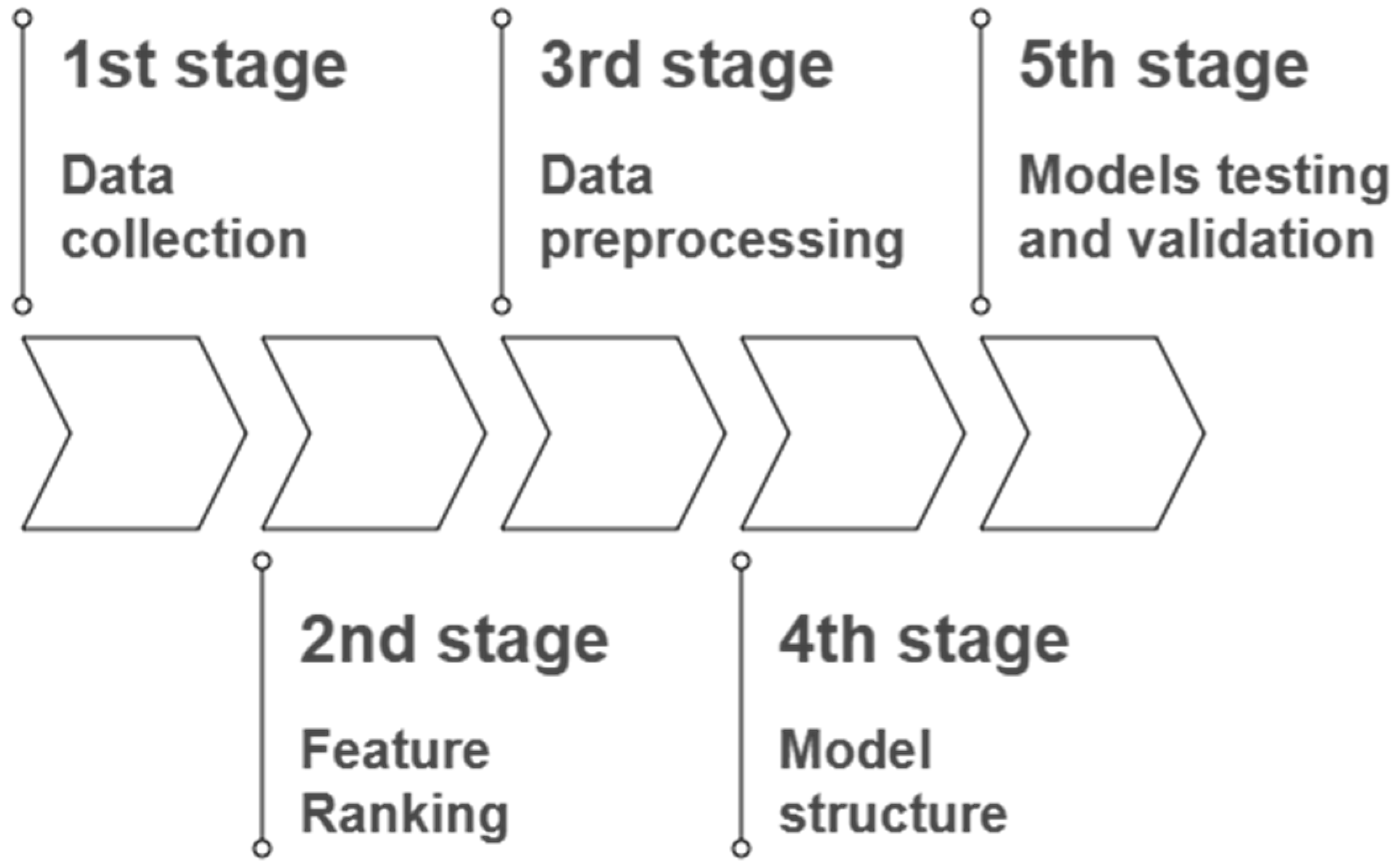
Figure 1. Structure of the used methodology.
Processes 13 02820 g001
Figure 2. Visualization of inter-variable relationships using a pair plot for the BHP prediction dataset.
Processes 13 02820 g002
Figure 3. Distribution of dataset parameters visualized through violin plots.
Processes 13 02820 g003
Figure 4. Ranking of dataset features by their effect on BHP-CTD.
Processes 13 02820 g004
Figure 5. Heatmap of Pearson correlation coefficients between dataset features relevant to BHP-CTD prediction.
Processes 13 02820 g005
Figure 6. Heatmap of Spearman correlation coefficients between dataset features relevant to BHP-CTD prediction.
Processes 13 02820 g006
Figure 7. A Pythagorean Forest diagram showing the range and structure of trees formed within a Random Forest.
Processes 13 02820 g007
Figure 8. Comparative heatmap of evaluation metrics for the applied machine learning models.
Processes 13 02820 g008
Figure 9. Predicted versus actual normalized BHP using a Neural Network trained with the L-BFGS optimizer.
Processes 13 02820 g009
Figure 10. Feature contribution assessment using SHAP in the Neural Network employing the L-BFGS optimization method.
Processes 13 02820 g010
Figure 11. Performance evaluation of multiple machine learning models using K-fold cross-validation.
Processes 13 02820 g011
Figure 12. Performance evaluation of multiple machine learning models using random sampling.
Processes 13 02820 g012
Figure 13. Comparison of measured pressures at coiled tubing depth with predicted pressures from various methods: (a) NN-LBFGS, (b) Hagedorn–Brown, (c) Beggs–Brill, (d) Orkiszewski, (e) Fancher–Brown, and (f) Duns–Ros.
Processes 13 02820 g013
Table 1. Summary statistics of the data collected.
ParameterUnitsMINMAXAVGMedian
Bottomhole pressure at coiled tubing depthpsi158594221411737
Fluid flow rate at surfacestb/d80451015521210
Water cut %01004150
Gas–oil ratioscf/stb02000609319
Water salinityppm49,995200,000150,941150,000
Wellhead flowing pressurepsi135708062
Wellhead flowing temperaturef72160103102
Coiled tubing depthft300013,04082508971
Nitrogen ratescf/m4001000519500
Oil gravityAPI12543735
Table 2. Compilation of machine learning and neural models along with the configuration choices applied.
ModelHyperparameters
GB-SKL
Total trees: 100
Learning step size: 0.1
Maximum tree depth: 3
Minimum subset size for splitting: 10
Training sample ratio: 0.8
XGB
Total trees: 200
Learning step size: 0.05
L2 regularization (lambda): 1
Maximum tree depth: 6
Training sample ratio: 0.8
Feature fraction per tree: 0.8
Feature fraction per level: 1.0
Feature fraction per split: 0.8
XGB-RF
Total trees: 200
Learning rate: 1
L2 regularization (lambda): 2
Maximum depth of trees: 5
Training sample ratio: 0.8
Features per tree: 0.7
Features per level: 1.0
Features per split: 0.8
GB-CB
Total trees: 100
Learning rate: 0.05
L2 penalty: 3
Maximum depth: 5
Feature subset for each tree: 0.8
ADAB
Number of estimators: 100
Learning rate: 0.05
Boosting type: SAMME.R (Real boosting)
Loss function (regression): squared error
RF
Size of forest: 10 trees
Number of attributes per split: 5
Maximum depth: 5
Minimum samples for splitting: 5
SVMs
SVM penalty parameter (C): 1
Epsilon for regression margin: 0.1
Kernel: Linear
Tolerance: 0.001
Max iterations: 1000
DT
Minimum leaf size: 15
Minimum split size: 7
Deepest allowable tree: 10
Stopping threshold: 95% of dominant class
KNN-D
k value: 5 neighbors
Distance metric: Euclidean
Weighting scheme: distance-based
KNN-U
k value: 5 neighbors
Distance metric: Euclidean
Weighting scheme: uniform
LR
Intercept term: included
Regularization type: Elastic Net
Alpha (regularization strength): 10
L1/L2 mix: 0.5: 0.5
NN-LBFGS
MLP (scikit-learn implementation)
Hidden layer size: 50 neurons
Activation function: ReLU
Optimizer: L-BFGS-B
Regularization weight: 0.01
Max iterations: 1000
NN-Adam
MLP (scikit-learn implementation)
Hidden layer size: 50 neurons
Activation function: ReLU
Optimizer: Adam
Regularization weight: 0.01
Max iterations: 1000
NN-SGD
MLP (scikit-learn implementation)
Hidden layer size: 50 neurons
Activation function: ReLU
Optimizer: SGD
Regularization weight: 0.01
Max iterations: 1000
SGD
Loss function: squared loss
Regularization: Elastic Net
Elastic Net mixing: 0.5
Regularization weight: 0.001
Learning rate strategy: constant
Number of training iterations: 1000
Table 3. Hyperparameter details for the symbolic regression models used.
ModelModel Parameters
GP-SR
The algorithm executes 100 iterations
Restricting expressions to a maximum size of 20
Table 4. Generated symbolic expressions with associated loss functions and model complexities.
ComplexityLossEquation
10.02577FFR_S
20.0204sin (FFR_S)
30.01902sin (sin (FFR_S))
40.00592 C T D F F R _ S
60.00484 ( F F R _ S + 0.1697795 ) C T D
70.00447(CTD + 0.26175192) (FFR _ S + 0.12106326)
80.00429sin ((FFR _ S + 0.112157054) (CTD + 0.32676274))
100.00396   FFR _ S   ( ( (   FFR _ S     GOR   ) + 0.85457504 )   CTD   )
110.00364 F F R _ S F F R _ S G O R + 0.75525254 C T D
130.00353 CTD ( FFR _ S ( ( FFR _ S G O R ) + s i n ( c o s ( W H T ) ) ) )
140.00346 C T D F F R _ S F F R _ S G O R + c o s ( s i n ( O G ) )
150.0034 ( (   FFR _ S     GOR   ) + c o s (   OG   ) ) ( (   FFR _ S     CTD   ) + 0.0032517365 )
160.00335 ( c o s ( s i n ( O G ) ) + (   FFR _ S G O R ) ) ( ( C T D F F R _ S ) + 0.0026609995 )
170.00303 c o s ( W S ) C T D ( ( ( W C + G O R ) + C T D ) W S ) + F F R _ S F F R _ S
180.00296 c o s ( W S ) C T D ( ( ( W C + s i n ( G O R ) ) + C T D ) W S ) + F F R _ S F F R _ S
190.00284 c o s ( W S ) F F R _ S + ( ( C T D + ( W C + G O R ) ) W S ) F F R _ S C T D + 0.0034129177
200.00271 c o s ( W S ) F F R _ S + ( ( ( C T D + W C ) + G O R ) s i n ( W S ) ) ( F F R _ S C T D ) + 0.004827395
Table 5. Dataset statistics from a sample of 29 wells.
ParameterUnitsMINMAXAVGMedian
Bottomhole pressure at coiled tubing depthPSI851378323042522
Fluid flow rate at surfaceSTB/D88357314371241
Water cut %01003730
Gas–oil ratioSCF/STB01556611500
Water salinityPPM51,000200,000143,451150,000
Wellhead flowing pressurePSI304909767
Wellhead flowing temperatureF90117104107
Coiled tubing depthFT300013,02886289002
Nitrogen rateSCF/M400750584600
Oil gravityAPI22463835
Table 6. Evaluation metrics for BHP-CTD prediction methods using MSE, RMSE, MAE, and R2.
BHP-CTD Prediction MethodsMSERMSEMAER2
Neural Network (L-BFGS)979199760.98
Hagedorn and Brown74,6002732120.91
Beggs and Brill107,2233272770.87
Orkiszewski117,1943422720.85
Fancher and Brown127,1483572950.84
Duns and Ros155,3313943250.81
Table 7. Comparative advantages and limitations of machine learning models versus traditional methods for BHP-CTD prediction.
ApproachAdvantagesLimitations
Machine Learning Models
High accuracy
Flexibility with a variety of well/reservoir conditions
Capability for real-time application
Resistant to missing/noisy data when preprocessed
Symbolic regression provides interpretable equations
Reliance on massive datasets of good quality
Possibility of retraining on the change in conditions
There are such models (e.g., neural networks), which are considered to be a black box
Empirical Correlations
Easy to apply
Low computation demands
Well recognized, and established in industry
Poor accuracies beyond original calibration range
Weak generalizability to variety of well conditions
Failure to model multidimensional interactions
Mechanistic Models
Physically grounded and interpretable
Able to simulate multiphase flow regimes
Widely validated in academic and industrial contexts
Demand many input parameters and calibration
Computationally demanding (particularly OLGA)
Limited feasibility for real-time field application
Disclaimer/Publisher’s Note: The statements, opinions and data contained in all publications are solely those of the individual author(s) and contributor(s) and not of MDPI and/or the editor(s). MDPI and/or the editor(s) disclaim responsibility for any injury to people or property resulting from any ideas, methods, instructions or products referred to in the content.