Fault Diagnosis Method for Rolling Bearings Based on a Digital Twin and WSET-CNN Feature Extraction with IPOA-LSSVM

Abstract

Rolling bearings, as essential parts of rotating machinery, face significant challenges in fault diagnosis due to limited fault samples and high noise interference, both of which reduce the effectiveness of traditional methods. To tackle this, this study proposes a fault diagnosis approach that combines Digital Twin (DT) and deep learning. First, actual bearing vibration data were collected using an experimental platform. After denoising the data, a high-fidelity digital twin system was built by integrating the bearing dynamics model with a Generative Adversarial Network (GAN), thereby effectively increasing the fault data. Next, the Wavelet Synchro-Extracting Transform (WSET) is used for high-resolution time-frequency analysis, and convolutional neural networks (CNNs) are employed to extract deep fault features adaptively. The fully connected layer of the CNN is then combined with a Least Squares Support Vector Machine (LSSVM), with key parameters optimized through an Improved Pelican Optimization Algorithm (IPOA) to improve classification accuracy significantly. Experimental results based on both simulated and publicly available datasets show that the proposed model has excellent generalizability and operational flexibility, surpassing existing deep learning-based diagnostic methods in complex industrial settings.

1. Introduction

Rolling bearings are widely utilized as critical components of mechanical equipment in various fields such as aerospace, transportation, and manufacturing [1]. Given that rolling bearing faults account for approximately 30% of the total rotating machinery failures, their standard forms of failure are wear, pitting, and cracking [2,3,4]. Bearing faults can directly result in mechanical damage or even catastrophic safety incidents, and the annual cost of maintaining bearings in the world reaches more than one billion dollars [5,6,7]. Therefore, accurate diagnosis of bearing faults is an important technology to prevent this disadvantage.

In recent years, with the rapid development of artificial intelligence, fault diagnosis has entered the era of significant data. Wang et al. [8] developed a Variational Autoencoder (VAE)-enhanced convolutional neural network (CNN) framework for rolling bearing fault diagnosis. It tackles challenges arising from noise, high-frequency variations, and redundancy in vibration signals. Xu et al. [9] proposed a model combining a convolutional neural network (CNN) and deep forest (gcForest), termed CNN-gcForest, to identify and capture the fault features of time-frequency vibration grayscale images of bearings. Liu et al. [10] proposed a multi-scale feature fusion approach to address the challenges of class imbalance and noise interference under limited sample conditions by leveraging twin networks. Guo et al. [11] combined wavelet transform with deep learning techniques for bearing fault diagnosis. Immovilli et al. [12] proposed the use of a long short-term memory network (LSTM) for bearing fault diagnosis. LSTM can capture long-term temporal features in signals and has a strong advantage in processing nonlinear, time-varying fault signals. The work of the above scholars mainly introduces deep learning to establish intelligent fault diagnosis models, which achieve automatic feature extraction and high-dimensional mapping through multi-layer structures. However, they did not consider the scarcity of bearing fault data samples, which resulted in the model being unable to converge during training and a decline in diagnostic capabilities. Moreover, Qin et al. [13] proposed a bearing fault data generation method based on a digital twin and Inverse Physics-Informed Neural Network (IPINN) to address the issue of insufficient and imbalanced samples for rolling bearing faults in practical engineering. Li et al. [14] proposed an innovative information-model adaptation method that combines the high-fidelity data generation capabilities of digital twins with the domain adaptation capabilities of transfer learning. Zhang et al. [15] utilized digital twins to generate high-fidelity simulation data and combined partial domain adaptation methods to address the issue of incomplete target domain categories under cross-operating conditions. Li et al. [16] employed a novel Deep Stacking Least Squares Support Vector Machine (DS-LSSVM) for rolling bearing fault diagnosis, combining non-parallel hyperplanes and a Least Squares Support Matrix Machine (LS-SMM), enabling the direct processing of matrix-form data and avoiding information loss caused by vectorization. Although the digital twins and deep learning methods studied by the above scholars have made significant progress in bearing fault diagnosis (such as in data augmentation, cross-condition adaptation, and the direct processing of matrix data), existing methods still face key issues such as significant deviations between generated data and real operating conditions, insufficient noise robustness, poor adaptability to small sample scenarios due to high model complexity, and dependence on manual parameter tuning.

Recently, swarm intelligence algorithms have shown great potential in fault diagnosis parameter optimization [17]. As a new meta-heuristic algorithm, the Pelican Optimization Algorithm (POA) has been applied to various engineering optimization problems due to its two-stage search mechanism (exploration–exploitation) [18]. For example, Tuervun et al. [19] combined the improved POA (IPOA) with a width learning system to achieve an accuracy rate of 98.75% in wind turbine fault classification; Sadeeq et al. [20] introduced Levy flight and improved exponential parameters to effectively enhance the performance of POA in function optimization and engineering design problems, addressing the drawback of the traditional POA getting stuck in local optima in high-dimensional complex problems; and SeyedGarmroudih et al. [21] introduced a knowledge-sharing factor and dimension-learning hunting (DHL) technology to solve the power system load allocation problem successfully. However, existing research has three limitations: (1) Most improvements to the POA only optimize a single stage (exploration or development), making it challenging to balance global search and local refinement. (2) In the field of bearing fault diagnosis, POA is mainly used for signal decomposition parameter optimization and has not yet been applied to the collaborative optimization of LSSVM kernel functions and regularization parameters. (3) Existing methods do not consider the high-dimensional characteristics of digital twin-generated data, resulting in insufficient parameter search efficiency.

In response to the above issues, a rolling bearing fault diagnosis model based on the integration of digital twins and deep learning methods is proposed. The core contributions of this paper can be summarized in the following four points:

1. It proposed a hybrid data generation framework based on digital twins and GANs, integrating bearing fault dynamics models and actual noise reduction data to solve the problem of scarce fault samples and generate data with high similarity to the distribution error of real data.

2. A collaborative analysis model combining WSET and CNN was designed. Wavelet synchronous transformation was used to enhance time-frequency resolution, and CNN was used to learn cross-scale fault features adaptively. The output of the CNN fully connected layer was used as input for the least squares support vector machine (LSSVM) to achieve end-to-end fault diagnosis.

3. The traditional Pelican Optimization Algorithm (POA) has been improved by introducing chaotic initialization, reverse differential evolution, and firefly disturbance mechanisms. Through the improved Pelican Optimization Algorithm (IPOA), the key parameters of LSSVM (regularization parameters and Gaussian kernel width) have been significantly optimized, greatly improving search and classification efficiency.

4. Experimental validation was conducted using simulation and public datasets (the University of Ottawa Bearing Failure Dataset), employing multi-dimensional metrics such as precision, recall, and F1 score, and utilizing statistical significance tests to verify the generalization capability and stability of the method.

The remainder of this paper is organized as follows: Section 2 introduces the overall model process; Section 3 describes the establishment of a digital twin model for bearing failures; Section 4 discusses the rolling bearing failure diagnosis model; Section 5 introduces the test dataset and validates the CNN-IPOA-LSSVM model; and Section 6 presents the conclusion.

2. Model Introduction

In this paper, a rolling bearing fault diagnosis model that fuses digital twin and deep learning is proposed, comprising a data generation module based on a digital twin and an intelligent rolling bearing diagnosis module. The primary process of the model is as follows:

(1) Leveraging digital twin technology for high-fidelity simulation data generation, this paper presents a hybrid enhancement approach that integrates physical mechanisms and measured data-driven methods to tackle the scarcity of rolling bearing fault samples. Based on the nonlinear dynamic model of the bearing constructed using Hertz contact theory, fault data involving inner and outer rings and rollers are generated via mathematical modeling simulation, thereby providing physical mechanism constraints for subsequent data generation. Simultaneously, actual bearing vibration signals are collected and processed for noise reduction to establish a high-quality data benchmark under real operating conditions. On this foundation, an improved generative adversarial network framework is designed, which innovatively incorporates both dynamics simulation data and measured data into the training process. The simulation data guarantees the physical plausibility of the generated results, while the measured data ensures the authenticity of the data through the supervised learning of the discriminator. This effectively overcomes the limitation of a single data source. The generated fault data not only conforms to the characteristics of bearing dynamics but also maintains a high level of consistency with the actual operating condition data, significantly enhancing the quality and diversity of the fault sample library.

(2) Time-frequency image generation and CNN feature extraction. To extract fault features from intricate vibration signals, this paper utilizes the Wavelet Synchro-Extracting Transform (WSET) to conduct modal decomposition on the collected fault signals, thereby generating time-frequency images. Time-frequency images are capable of simultaneously capturing the time-domain and frequency-domain characteristics of signals, offering copious fault information. The dimension-reduced time-frequency images are input into a two-dimensional convolutional neural network (2D-CNN) for fault feature extraction. Through multiple convolutional layers and pooling layers, the CNN progressively extracts local features within the time-frequency images and maps the extracted features to a high-dimensional space via fully connected layers. The automatic feature extraction of the CNN can effectively capture the deep-seated features in fault signals.

(3) To enhance the classification performance of the Least Squares Support Vector Machine (LSSVM), this study presents an Improved Pelican Optimization Algorithm (IPOA) for optimizing the crucial parameters (regularization parameter and Gaussian kernel width) of the LSSVM. The IPOA is founded on the traditional Pelican Optimization Algorithm (POA) and incorporates three key improvement aspects:

(1) Population initialization based on logistic chaos mapping: The initial population is generated via logistic chaos mapping to guarantee that the initial solutions are uniformly distributed within the search space. Its randomness and unpredictability can effectively cover the entire solution space, thus circumventing the local optimization issue that might be induced by the traditional random initialization method.

(2) Oppositional Differential Evolution (ODE): During the iterative process, reverse learning is introduced to generate the reverse solution to expand the search scope. By comparing the fitness of the original solution with that of the reverse solution, the superior individual is retained to prevent the algorithm from getting trapped in local optimality.

(3) Firefly perturbation mechanism: Inspired by the attraction mechanism of the firefly algorithm, a perturbation is applied to an individual to assist it in moving towards a more optimal solution. The firefly perturbation enhances the local search capability of the algorithm, which can fine-tune the solution during the development stage and further enhance the optimization effect.

(4) End-to-end fault diagnosis. The feature vectors extracted by the fully connected layers of the CNN are utilized as the input of the LSSVM. In combination with the LSSVM parameters optimized by the IPOA, an end-to-end fault diagnosis model is established. The LSSVM maps nonlinear problems to high-dimensional spaces via kernel functions, processes intricate nonlinear data, and balances model complexity and training errors through regularization parameters to prevent overfitting. This model can effectively segregate fault features from complex, noisy signals and attain high-precision fault classification. The flowchart of the model is presented in Figure 1.

3. Rolling Bearing Fault Modeling Based on Digital Twins

This paper develops a digital twin model via the dynamic modeling of rolling bearings and an enhanced Generative Adversarial Network (GAN) to address the shortage of fault samples. Initially, a nonlinear dynamic model is formulated based on the physical attributes of bearings to simulate the vibration responses of inner race, outer race, and rolling element faults. Subsequently, an improved GAN approach is presented, in which the denoised measured data are used to train the discriminator to enhance the quality of the generated data. The generator produces data, and the discriminator distinguishes between real and generated data. Through adversarial training, simulation data that are highly consistent with the actual data distribution are generated. Finally, the accuracy of the model is verified through numerical computations to ensure that the generated data accurately reflect the actual fault characteristics. This technology provides sufficient training data for the subsequent CNN-IPOA-LSSVM fault diagnosis model, enabling precise diagnosis under complex operating conditions.

3.1. Dynamic Model of Rolling Bearings

To investigate the failure of the bearing system, this paper formulates the following assumptions: The mass-spring-damping model is employed to depict the dynamics of the bearing. Contact deformation is analyzed based on Hertz contact theory. The outer ring is fixed, and the outer-ring raceway is considered rigid. The inner ring rotates synchronously with the shaft without slippage, and there is also no slippage phenomenon for the rolling elements within the raceway. Currently, the model does not account for the effects of cages, lubricating oil, and temperature rise. A dynamic model of the rolling bearing, as shown in Figure 2, is established.

Based on the above assumptions, the vibration response of rolling bearings can be described by a four-degree-of-freedom dynamic equation, corresponding to the movements of the inner and outer rings in the x and y directions:

$$\left\{\begin{array}{l}{m}_i{\ddot{x}}_i+c_{ix}{\dot{x}}_i+k_{ix}{x}_i=-F_{ix}+m_{i}e{\omega }^2\cos (\omega t)+W_x\\ m_i{\ddot{y}}_i+c_{iy}{\dot{y}}_i+k_{iy}{y}_i=-F_{iy}+m_{i}e{\omega }^2\sin (\omega t)-m_{i}g+W_y\\ m_o{\ddot{X}}_o+c_{ox}{\dot{X}}_o+k_{ox}{x}_o=F_{ox}\\ m_o{\ddot{y}}_o+c_{oy}{\dot{y}}_o+k_{oy}{y}_o=F_{oy}-m_{o}g\end{array}\right.$$

(1)

where, m_i and m_o are the masses of the inner and outer rings; c_ix, c_iy, c_ox, and c_oy are damping coefficients; k_ix, k_iy, k_ox, and k_oy are support stiffnesses; F_ix, F_iy, F_ox, and F_oy are nonlinear contact forces between rolling elements and raceways; W_x and W_y are radial forces applied to the bearing; and $\omega$ is the angular velocity.

The contact force between the rolling body and raceway is calculated based on the Hertz contact theory, where the contact deformation of the jth rolling body is as follows:

$${\delta }_j=(x_i-x_o)\cos {\theta }_j+(y_i-y_o)\sin {\theta }_j-c_d-h$$

(2)

where c_d is the bearing clearance correction term with value $c_d=0.5c_r\left[1-\cos \left({\displaystyle \frac{3\pi }{2}}-{\theta }_j\right)\right]$, and h is the time-varying displacement excitation due to failure (h = 0 in healthy state).

The equivalent contact stiffness k_b of the rolling body with the inner and outer rings is as follows:

$$k_b={\left[{\displaystyle \frac{1}{{\left(1/k_{bi}\right)}^{2/3}+{\left(1/k_{bo}\right)}^{2/3}}}\right]}^{\frac{3}{2}}$$

(3)

in which k_bi and k_bo are the contact stiffness of the rolling body with the inner and outer rings, respectively, and are calculated by the following formula:

$${\mathrm{k}}_{bi}={\displaystyle \frac{2\sqrt{2}}{3}}\left({\displaystyle \frac{E}{1-{\mu }^2}}\right){\left({\delta }_i^{\ast }\right)}^{-\frac{3}{2}}{\left({\displaystyle \sum {\rho }_i}\right)}^{\frac{1}{2}}$$

(4)

$$k_{bo}={\displaystyle \frac{2\sqrt{2}}{3}}\left({\displaystyle \frac{E}{1-{\mu }^2}}\right){({\delta }_o^{\ast })}^{-\frac{3}{2}}{\left({\displaystyle \sum {\rho }_o}\right)}^{\frac{1}{2}}$$

(5)

where ${\displaystyle \sum {\rho }_i}$, ${\displaystyle \sum {\rho }_o}$ are the sum of the principal curvatures of the inner and outer rings, and ${\delta }_i^{\ast }$ and ${\delta }_o^{\ast }$ are the parameters of the curvature difference function (taken from Rolling Bearing Analysis (5th ed.) [22]).

The nonlinear bearing contact force based on Hertz contact theory is as follows:

$$F_x={\displaystyle \sum _{j=1}^{N_b}{k}_b{\delta }_j^{\frac{3}{2}}H\left({\delta }_j\right)\cos {\theta }_j}$$

(6)

$$F_y={\displaystyle \sum _{j=1}^{N_b}{k}_b{\delta }_j^{\frac{3}{2}}H\left({\delta }_j\right)\cos {\theta }_j}$$

(7)

where N_b is the number of bearing rollers and $H\left({\delta }_j\right)$ is the Heaviside function, which determines whether contact has occurred: $H\left({\delta }_j\right)=\left\{\begin{array}{ll}1& {\delta }_j>0\\ 0& {\delta }_j\le 0\end{array}\right.$.

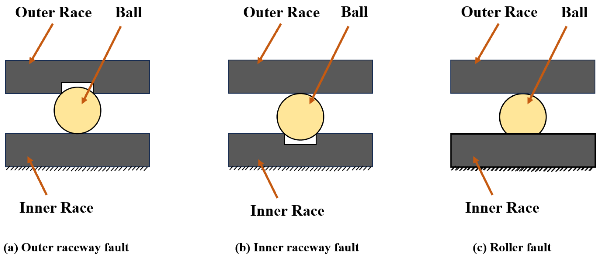
Three types of rolling bearing fault forms are simulated in this model, namely, outer ring failure, inner ring failure, and rolling element failure, whose localized failure forms are simulated as rectangular shedding, as shown in Figure 3.

Consider the time-varying displacement excitation, as shown in Figure 3a, with the geometric angle of the outer ring contact point:

$${\phi }_{do}=\arcsin {\displaystyle \frac{L}{D_{out}}}$$

(8)

where L denotes the width of the outer ring defect, and D_out denotes the diameter of the outer ring.

The phase angle of a rolling body can be expressed as follows:

$${\phi }_o=\mathrm{mod}({\theta }_j,2\pi )$$

(9)

where ${\theta }_{\mathrm{j}}$ denotes the position angle of the system at a given moment.

The maximum displacement of the rolling body can be expressed as follows:

$${\Delta }_{\max }={\displaystyle \frac{D_b}{2}}-\sqrt{{({\displaystyle \frac{D_b}{2}})}^2-{({\displaystyle \frac{L}{2}})}^2}$$

(10)

where D_b is the diameter of the roller, and L is the width of the outer ring defect.

Thus, the excitation displacement describing the outer ring fault condition can be expressed as follows:

$$h_{\mathrm{out}}=\left\{\begin{array}{lll}{\Delta }_{max}+{\Delta }_{max}\sin {\displaystyle \frac{{\phi }_o-{\phi }_{os}}{2{\phi }_{do}}}\pi \hfill & {\phi }_{os}-{\phi }_{do}\le {\phi }_o<{\phi }_{os}\hfill & \\ {\Delta }_{max}\hfill & {\phi }_o={\phi }_{os}\hfill & \\ {\Delta }_{max}-{\Delta }_{max}\sin {\displaystyle \frac{{\phi }_o-{\phi }_{os}}{2{\phi }_{do}}}\pi \hfill & {\phi }_{os}<{\phi }_o\le {\phi }_{os}+{\phi }_{do}\hfill & \\ 0\hfill & \mathrm{else}\hfill & \end{array}\right.$$

(11)

where ${\phi }_{os}$ denotes the phase angle of the outer ring fault, and its value is taken as ${\displaystyle \frac{11}{6}}\pi$, ${\displaystyle \frac{5}{3}}\pi$, ${\displaystyle \frac{3}{2}}\pi$, ${\displaystyle \frac{4}{3}}\pi$, ${\displaystyle \frac{7}{6}}\pi$.

Similarly, the excitation displacements for the inner ring fault in Figure 3b and the rolling body fault in Figure 3c are as follows:

$$h_{in}=\left\{\begin{array}{lll}{\Delta }_{max}+{\Delta }_{max}\sin {\displaystyle \frac{{\phi }_i-{\phi }_{is}}{2{\phi }_{di}}}\pi \hfill & {\phi }_{is}-{\phi }_{di}\le {\phi }_i<{\phi }_{is}\hfill & \\ {\Delta }_{max}\hfill & {\phi }_i={\phi }_{is}\hfill & \\ {\Delta }_{max}-{\Delta }_{max}\sin {\displaystyle \frac{{\phi }_i-{\phi }_{is}}{2{\phi }_{di}}}\pi \hfill & {\phi }_{is}<{\phi }_i\le {\phi }_{is}+{\phi }_{di}\hfill & \\ 0\hfill & \mathrm{else}\hfill & \end{array}\right.$$

(12)

$$h_{\mathrm{ball}}=\left\{\begin{array}{lll}{\Delta }_{max}\hfill & -{\phi }_{db}\le {\phi }_b<{\phi }_{db}\hfill & \\ {\Delta }_{max}\hfill & -{\phi }_{db}\le {\phi }_b-\pi <{\phi }_{db}\hfill & \\ 0\hfill & \mathrm{else}\hfill & \end{array}\right.$$

(13)

By using these formulas, the vibration response of a bearing under any operating conditions can be calculated directly by the Runge–Kutta method, which is more efficient and convenient compared to laboratory experiments.

3.2. Dynamic Model Validation

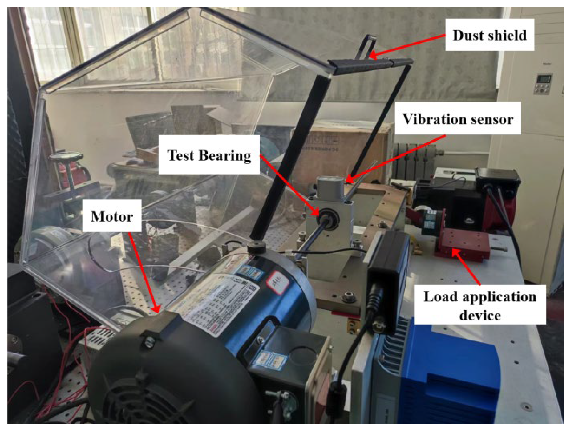
To validate the efficacy of the proposed digital twin model, this research employs a combination of theoretical computation and experimental verification to corroborate the bearing dynamics model systematically. This study leverages the bearing test bench of Shenyang Architecture University to gather real-world data, as depicted in Figure 4. The primary objective of this research is to provide the discriminator with training samples that feature typical fault characteristics, following noise reduction processing of the collected data, thereby ensuring consistency between the generated data and the real-data distribution. The experimental system comprises a servo motor, a drive shaft, a bearing test unit, and a data acquisition system. The servo motor is connected to the drive shaft with a diameter of 12.7 mm via an elastic coupling, which effectively mitigates the interference of motor vibration on the test signal. The test bearing is of model 6205, and the specific data are presented in

Table 1. Parameters of the 6205 bearing.

Parameter	Value
Inner roller diameter (Di/mm)	25
Outer roller diameter (Db/mm)	52
Pitch diameter (Dw/mm)	38.5
Rolling diameter (db/mm)	7.9
Number of rolling (Z)	9
Clearance diametral (Cr)	1
Rolling quality (m0/g)	2.14

. Its inner ring is in close fit with the drive shaft, while the bearing housing fixes the outer ring. A high-frequency acceleration sensor is installed at the top center of the bearing housing at a sampling rate of 102.4 kHz to collect vibration signals in real-time. The collected data are transferred to a computer for storage and analysis after 24-bit analogue-to-digital conversion. During the experiment, three bearing fault conditions, namely outer ring fault (OF), inner ring fault (IF), and ball fault (BF), as well as normal conditions, were manually customized for a total of four health conditions.

Based on the established dynamics model, numerical simulations were carried out for four working conditions, namely, healthy state, outer ring failure, inner ring failure, and rolling element failure, respectively. The vibration signals obtained through numerical calculation were compared with the theoretical values, as shown in

Table 2. Fault characteristic frequency result error.

Fault Condition	Damage Diameter/mm	Theoretical Fault Eigenfrequency/Hz	Model Fault Eigenfrequency/Hz	Inaccuracy/%
IF	0.5	162.187	162.182	0.003
OF		107.336	107.273	0.06
BF		69.523	69.454	0.09

. Among them, the characteristic frequency error of the inner ring failure is only 0.003%, and the mistakes of the outer ring and rolling element failures are controlled within 0.06% and 0.09%, respectively, which indicates that the model can accurately reflect the fault characteristics of the bearing.

To improve the quality of the generated data, the bearing vibration signals under actual working conditions were experimentally collected. By comparing the data distribution before and after noise reduction, as shown in Figure 5, it can be seen that the noise reduction treatment effectively retains the fault characteristics and provides high-quality benchmark data for subsequent GAN training. The synergistic use of measured data and simulation data ensures both the physical reasonableness of the generated data and its consistency with the actual working conditions, providing reliable data support for the training of the fault diagnosis model.

3.3. Digital Twin-Based Fault Data Generation

To address the issue of poor discriminator training performance resulting from noise interference in actual bearing vibration signals, this paper proposes a discriminator training method based on noise-reduced data. Under the GAN framework, the actual data processed through noise reduction is used as the true sample p_denoised of the discriminator D, and the data generated by the generator G is used as the negative sample.

The objective function of the discriminator is defined as follows:

$${\mathcal{L}}_D={\mathbb{E}}_{x\sim p_{\mathrm{denoised}}}[\log D(x)]+{\mathbb{E}}_{z\sim p_z}[\log (1-D(G(z)))]$$

(14)

The objective function of the generator is defined as follows:

$${\mathcal{L}}_G={\mathbb{E}}_{z\sim p_z}[\log (1-D(G(z)))]$$

(15)

The core advantage of this method is that by introducing noise-reduced real data to train the discriminator, it can effectively avoid the interference of noise in actual measurements on the performance of the discriminator, enabling the discriminator to more accurately learn the distribution characteristics of fault features, thereby significantly improving the quality of the generated data and producing simulation data with a high degree of similarity to real fault data, as shown in Figure 6.

4. Rolling Bearing Fault Diagnosis Model

In response to the issue of complex noise interference with fault signals under practical working conditions, this paper presents a fault diagnosis model. This model is based on the Improved Pelican Optimization Algorithm (IPOA) for optimizing the Least Squares Support Vector Machine (LSSVM) and is combined with the convolutional neural network (CNN). The model generates high-fidelity simulation data via digital twin technology, employs a CNN to extract fault features adaptively, and optimizes the key parameters of LSSVM through IPOA to enhance classification accuracy and robustness. The model process is shown in Figure 7, and the specific implementation steps are as follows:

(1) Data preprocessing: the original vibration signal is normalized, and a sliding window segmentation is used to generate the sample sequence;

(2) Image processing for dimensionality reduction: a Wavelet Synchro-Extracting Transform (WSET) is used to convert the time domain signal into a time-frequency image, 95% of the energy components are retained by principal component analysis (PCA), and a normalized feature image of 64 × 64 × 3 is output;

(3) CNN feature extraction: a deep network containing two layers of convolution and pooling is constructed, with 16 3 × 3 convolution kernels in the first layer and 32 5 × 5 convolution kernels in the second layer, and multilevel fault features are extracted by the Relu activation function and the maximum pooling operation;

(4) Intelligent classification decision-making: the feature vectors output from the fully connected layer of the CNN are fed into the LSSVM classifier, and the improved IPOA algorithm is used to optimize the regularization parameter and the width of the Gaussian kernel of the LSSVM, to achieve high-precision fault classification.

4.1. Data Processing Method Based on WSET-CNN

This study collects rolling bearing fault data in real time using digital twin technology. The raw vibration signals are preprocessed to extract fault features effectively. We employ the Wavelet Synchro-Extracting Transform (WSET) [23] for modal decomposition. WSET overcomes the time-frequency resolution limitations of traditional wavelet transforms and enhances signal features through synchronous extraction. The procedure is as follows:

(1) The original vibration signal is transformed using WSET to obtain a time-frequency representation. Based on the continuous wavelet transform, WSET is defined as follows:

$$W_x(a,\tau )={\displaystyle \frac{1}{\sqrt{a}}}{\displaystyle {\int }_{-\infty }^{\infty }x}(t){\psi }^{\ast }\left({\displaystyle \frac{t-\tau }{a}}\right)dt$$

(16)

where x(t) is the input signal, $\psi \left(t\right)$ is the mother wavelet, a is the scale parameter (inversely proportional to the frequency), and $\tau$ is the time translation parameter (time offset).

The WSET transformation expressions are as follows:

$$\mathrm{WSET}(t,f)=W_x(a,\tau )\cdot \delta \left(f-\widehat{f}(t)\right)$$

(17)

where f(t) is the instantaneous frequency estimate of the signal and δ(⋅) is the Dirac function (used to filter specific frequency components).

(2) WSET decomposes the signal into k modal components, each representing a distinct frequency band, to separate fault features initially:

$$x(t)={\displaystyle \sum _{k=1}^K{M}_k}(t)+r(t)$$

(18)

where $M_k\left(t\right)$ is the kth modal component, and $r(t)$ is the residual component.

(3) The decomposed modal components are transformed into time-frequency images for subsequent processing.

(4) Since the time-frequency images obtained after WSET decomposition have high dimensionality, directly inputting them into a convolutional neural network (CNN) would increase computational complexity. Therefore, this paper uses principal component analysis (PCA) to reduce the dimensionality of the time-frequency images [24]. After flattening the images from WSET decomposition into one-dimensional vectors, PCA is applied to retain the main feature components and minimize data redundancy. The reduced-dimensionality data are then reshaped into a 64 × 64 × 3 two-dimensional time-frequency image for input into the CNN.

4.2. Improved Pelican Optimization Algorithm

The Pelican Optimization Algorithm (POA) was proposed by Pavel Trojovský et al. [25]. This algorithm mimics the natural behavior of pelicans during hunting and updates candidate solutions by simulating the pelican’s feeding strategy to solve optimization problems in engineering applications. Population initialization is a key process in swarm intelligent optimization algorithms. In the POA, individuals are randomly generated within a specified range during population initialization. The high level of randomness and uncertainty in the initial individuals affects the algorithm’s convergence speed and the outcome of the optimization search. To address this issue, this paper introduces three improvement points.

(1) Population initialization using logistic chaotic mapping [26]. Chaotic initialization through logistic mapping ensures a more uniform distribution of initial solutions across the search space. The inherent randomness and unpredictability of chaotic maps facilitate better coverage of the solution domain. The logistic mapping is defined as follows:

$$x_{n+1}=\mu x_n(1-x_n)$$

(19)

where $\mu$ is the control parameter, $x_n$ is the current value, and $x_{n+1}$ is the next value.

(2) The incorporation of Oppositional Differential Evolution (ODE) [27]. To mitigate the risk of converging to local optima, a reverse learning mechanism is integrated into the iterative process. For each current solution x, an inverse solution x′ is generated according to the following:

$$x_i^{\prime }=a+b-x_i$$

(20)

where a and b denote the lower and upper bounds of the search space, respectively. The fitness values of the original and inverse solutions are compared, and the superior individual is retained.

(3) Firefly algorithm perturbation (FAP) [28]. The traditional POA development stage may not be able to fine-tune the solution due to insufficient local search capability. Firefly perturbation, which draws on the attraction mechanism of the firefly algorithm, applies perturbation to individuals to help them move towards a better solution. Its mathematical expression is as follows:

$$X_{\mathrm{hf}}(i,:)=X(i,:)+\beta \cdot e^{-\gamma r^2}\cdot \left(X_{\mathrm{best}}-X(i,:)\right)+\alpha \cdot ϵ$$

(21)

where X_best is the current optimal solution, β is the attraction coefficient, $\gamma$ is the light absorption coefficient, r is the distance between the two individuals, $\alpha$ is the random step size, and $ϵ$ is the random vector.

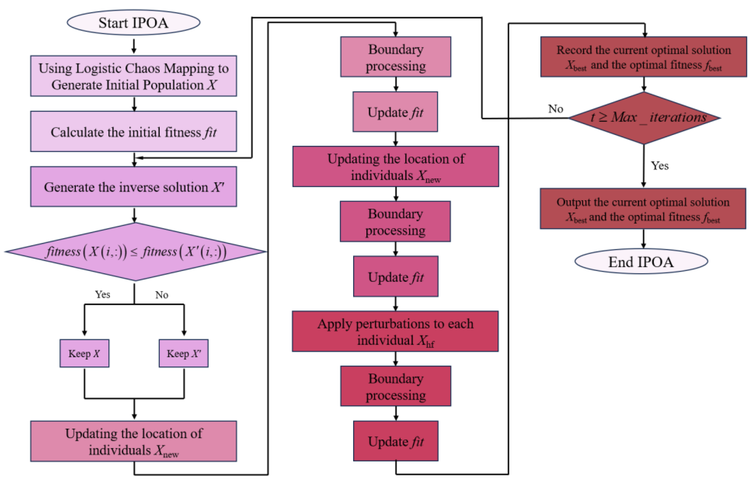
The algorithm is divided into two phases: approaching prey (exploration phase), and surface flight (exploitation phase). The flowchart of the algorithm is shown in Figure 8, and the details of the process are as follows:

(1) Initialization. Generate chaotic sequences $x_1,x_2,\cdots x_N$ from Equation (19). Map the chaotic sequences to the solution space to obtain the initial population:

$$X(i,j)=lowerbound(j)+x_{n+1}\cdot (upperbound(j)-lowerbound(j))$$

(22)

where X(i,j) is the jth dimensional position of the ith individual, and lowerbound (j) and upperbound (j) are the upper and lower bounds of the jth dimension.

Calculate the initial fitness fit with the following formula:

$$fit(i)=fitness\left(X(i,:)\right)$$

(23)

(2) Opposite Difference Evolution (ODE). Generate the inverse solution $X^{\prime }$:

$$X^{\prime }\left(i,j\right)=lowerbound\left(j\right)+upperbound\left(j\right)-X\left(i,j\right)$$

(24)

Compare the fitness of the original and inverse solutions and retain the better solution:

$$X(i,:)=\left\{\begin{array}{lll}X(i,:)\hfill & fitness(X(i,:))\le fitness(X^{\prime }(i,:))\hfill & \\ X^{\prime }(i,:)\hfill & else\hfill & \end{array}\right.$$

(25)

(3) Approaching prey (exploration phase). In this phase, the pelican determines the location of its prey and then moves towards this determined area. Modeling the pelican’s approaching prey strategy allows it to scan the search space, which in turn leverages the algorithm’s ability to explore different regions in the search space. The exploration phase updates the location of the individual:

$$X_{new}\left(i,:\right)=X\left(i,:\right)+rand(1,1)\cdot \left(X_{Food}-I\cdot X\left(i,:\right)\right)$$

(26)

where X_Food is the food source location (randomly selected individuals), rand(1,1) is a random number in the range [0, 1], and I is a random integer of 1 or 2.

Boundary processing is performed to avoid the solution vectors going beyond the predefined upper and lower bounds:

$$\left\{\begin{array}{l}{X}_{\mathrm{new}}(i,j)=max\left(X_{\mathrm{new}}(i,j),lowerbound(j)\right)\\ X_{\mathrm{new}}(i,j)=min\left(X_{\mathrm{new}}(i,j),upperbound(j)\right)\end{array}\right.$$

(27)

Updating adaptation:

$$fit(i)=\left\{\begin{array}{lll}fitness(X_{\mathrm{new}}(i,:))\hfill & fitness(X_{\mathrm{new}}(i,:))\le fit(i)\hfill & \\ fit(i)\hfill & else\hfill & \end{array}\right.$$

(28)

(4) Surface flight (developmental stage). At this stage, when pelicans reach the water surface, they extend their wings over the water, lift the fish upwards, and then transfer the prey into their throat pouches. This surface-flight strategy used by pelicans allows them to catch more fish within the targeted area. Following this strategy to update their individual positions, the expression is as follows:

$$X_{\mathrm{new}}(i,:)=X(i,:)+0.2\cdot \left(1-{\displaystyle \frac{t}{Max\_iterations}}\right)\cdot (2\cdot \mathrm{rand}(1,dimension)-1)\cdot X(i,:)$$

(29)

where t is the current number of iterations, Max_iterations is the maximum number of iterations, and rand(1,dimension) is a random vector in the range [0, 1]. Same as above for boundary processing and updating the fitness.

(5) Firefly perturbation. A perturbation is applied to each individual by Equation (21), and boundary processing and updating of fitness are performed as above.

(6) Update the optimal solution. Record the current optimal solution fbest = min(fit) and the fitness X_best = X(argmin(fit),:).

(7) Output result.

4.3. The CNN-IPOA-LSSVM Model

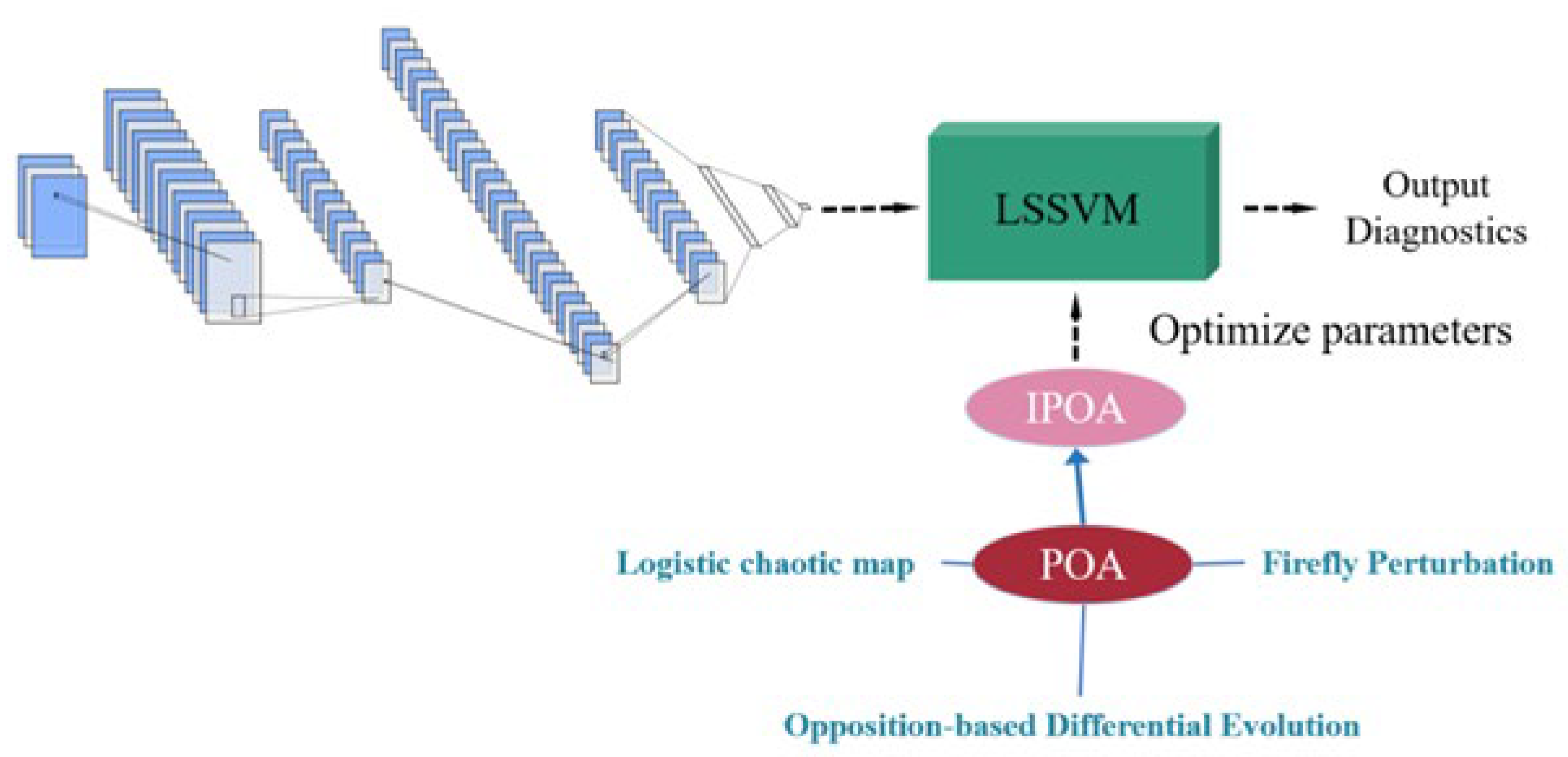
The CNN-IPOA-LSSVM model presented in this paper is illustrated in Figure 9 below.

To further extract fault features, this study employs a two-dimensional convolutional neural network (2D-CNN) for adaptive feature extraction on reduced-dimension time-frequency images [29]. Figure 10 illustrates the CNN architecture designed in this paper. Table 3 presents the parameters of the convolutional neural network used in this model. Given the specific requirements of bearing fault diagnosis, the advantages of the CNN architecture designed in this paper (input layer → two convolutional pooling layers → three fully connected layers) are as follows:

(1) The first layer uses 16 3 × 3 small convolutional kernels, which can effectively capture the transient features of weak faults;

(2) The second layer innovatively employs 2 × 1 asymmetric pooling, preserving the temporal integrity of the vibration signal while reducing dimensionality, making it more suitable for variable speed operating conditions;

(3) The stepped fully connected layers (64 → 32 → 4) are combined with the LSSVM input requirements to prevent overfitting with small samples.

Table 3. Designed CNN network structure and function.

Network Layer	Kernel Size/STRIDE	Channels/UNITS	Output Size	Function
Input layer	/	3	64 × 64 × 3	/
Conv_1	3 × 3/1	16	64 × 64 × 16	Relu
MaxPool_1	2 × 2/2	16	32 × 32 × 16	MaxPooling
Conv_2	5 × 5/1	32	32 × 32 × 32	Relu
MaxPool_2	2 × 1/2	32	16 × 32 × 32	MaxPooling
Flatten	/	/	16,384	Convert map into vector
FC1	/	64	1 × 1 × 64	Relu
FC2	/	32	1 × 1 × 32	Relu
FC3	/	4	1 × 1 × 4	Softmax

Table 3. Designed CNN network structure and function.

Network Layer	Kernel Size/STRIDE	Channels/UNITS	Output Size	Function
Input layer	/	3	64 × 64 × 3	/
Conv_1	3 × 3/1	16	64 × 64 × 16	Relu
MaxPool_1	2 × 2/2	16	32 × 32 × 16	MaxPooling
Conv_2	5 × 5/1	32	32 × 32 × 32	Relu
MaxPool_2	2 × 1/2	32	16 × 32 × 32	MaxPooling
Flatten	/	/	16,384	Convert map into vector
FC1	/	64	1 × 1 × 64	Relu
FC2	/	32	1 × 1 × 32	Relu
FC3	/	4	1 × 1 × 4	Softmax

Figure 10. Structure of the designed CNN.

Figure 10. Structure of the designed CNN.

The CNN-extracted features (from FC3) are fed into an LSSVM for classification. LSSVM uses kernel functions to handle nonlinearity and regularization to avoid overfitting. Its performance depends on two key parameters: the regularization parameter C and the Gaussian kernel width σ.

Therefore, to improve classification accuracy and robustness, this paper uses the improved pelican optimization algorithm (IPOA) proposed in Section 4.2 to perform global optimization of the C and σ parameters of LSSVM. IPOA searches for the optimal parameter combination to enable LSSVM to achieve the best classification performance on the given CNN features.

The final decision function is as follows:

$$f(x)={\displaystyle \sum _{i=1}^N{\alpha }_i}K(x,x_i)+b$$

(30)

where ${\alpha }_i$ is the Lagrange multiplier, K(x, x_i) is the kernel function, and b is the bias term.

4.4. Simulation Result

To validate the simulation data using the model proposed in this paper, the first 170 samples of each dataset are used as the training set, and the remaining samples as the test set. The output labels are converted into classification labels (the twin dataset contains 1000 samples, with the 1st–250th representing the inner ring fault features, the 251st–500th representing the outer ring fault features, the 501st–750th representing the rolling body fault features, and the 751st–1000th representing the normal features) for supervised learning in the model.

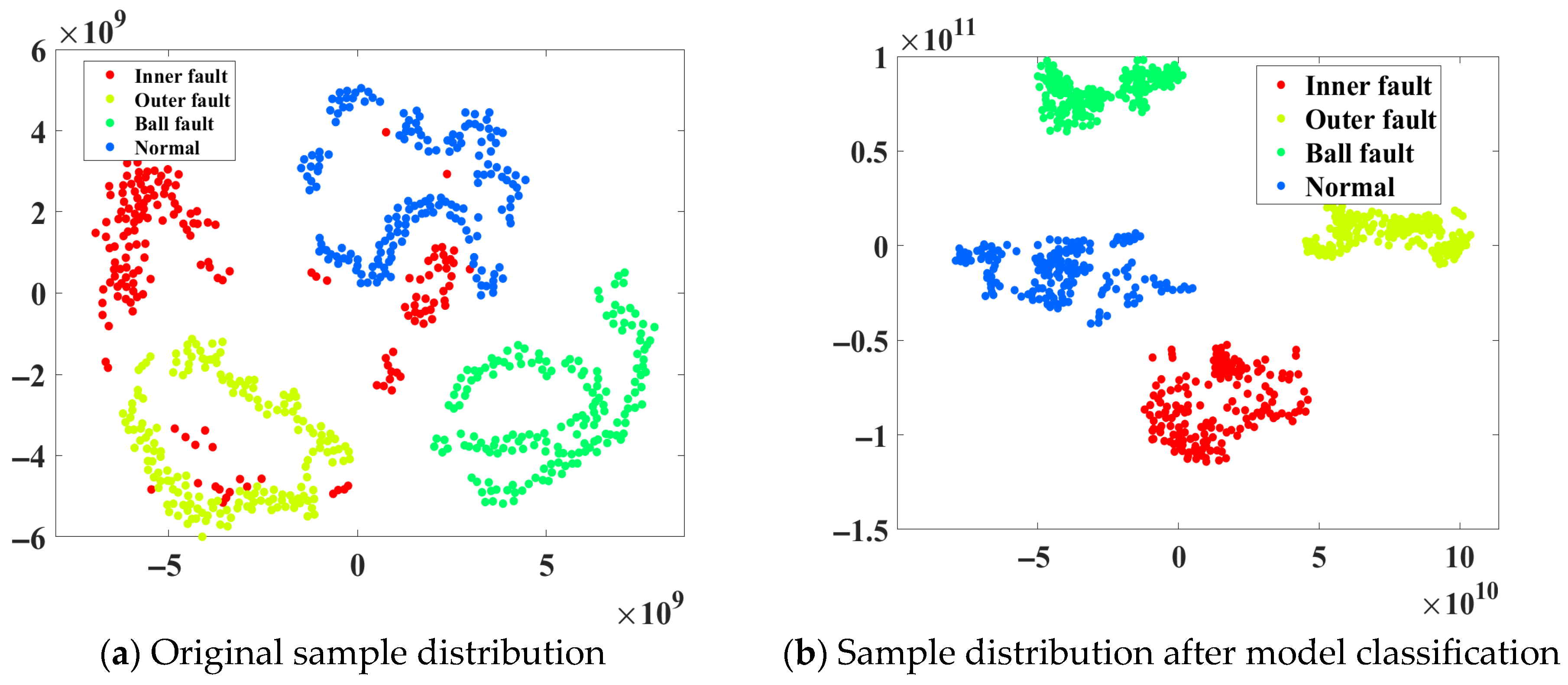
In the model, CNN automates the extraction of high-level features from the original data, reducing the need for manual feature engineering. The IPOA identifies the optimal parameters of LSSVM through an intelligent optimization algorithm to enhance classification performance. LSSVM then uses the optimized parameters to perform classification with high computational efficiency and accuracy, as shown in Figure 11 and Figure 12.

The classification of twin samples after model identification is shown using t-SNE visualization. It can be seen that the model plays an excellent role in classifying different types of faults.

The diagnostic accuracy of this model on the simulated dataset was visualized using the confusion matrix. It was observed from the matrix that a diagnostic accuracy of 99.68% was achieved, enabling highly precise fault detection.

5. Experimental Validation

5.1. Dataset Description

In actual industrial scenarios, bearings usually operate under complex variable conditions. Specifically, changes in rotational speed can significantly affect fault signal characteristics, making fault diagnosis more challenging. Therefore, conducting experiments with variable rotational speeds can better simulate real-world working conditions, test the model’s adaptability and robustness across different speeds, and improve the practicality and reliability of the fault diagnosis method. This paper uses the University of Ottawa bearing dataset (Ottawa) [30] for testing. To evaluate model stability, all experiments are repeated five times independently, and the average results and standard deviations are reported. Considering the stochastic nature of rolling element contact on the raceway, the bearing conditions in the experiment are defined as follows: healthy, inner ring failure (IF), outer ring failure (OF), and roller failure (BF). The details of the bearings used for testing are shown in

Table 4. Ottawa dataset test bearing information.

Bearing Parameter
Bearing type	ER16K
Inner ring diameter/mm	25.04
Outer ring diameter/mm	52.07
Number of rollers	9
Roller diameter/mm	7.94
Pitch diameter/mm	39.04
Contact angle/°	0

.

The publicly available University of Ottawa (Ottawa) bearing dataset contains vibration signals for a variety of failure types and at different rotational speeds. The dataset provides failure data for ER16K bearings in various states under variable operating conditions, and the experimental states under variable operating conditions are shown in

Table 5. Ottawa experimental bearing status data.

Working Condition Type		Motor RPM/r·min−1
A1	Accelerating	846-1428
B1	Decelerating	1734-822
C1	Accelerating then decelerating	882-1518-1260
D1	Decelerating then accelerating	1452-888-1236

.

The raw time-domain vibration signals were collected with a 2-channel data logger at a sampling frequency of 200 kHz for not less than 10 s for each fault condition. The experiments were conducted on a SpectraQuest Mechanical Failure Simulator (MFS-PK5M), and the experimental setup is shown in Figure 13.

The test rig consists of a motor, AC drive, encoder, coupling, rotor, and bearings. The Ottawa bearing dataset is used in this paper to test the diagnostic accuracy of the proposed method under variable operating conditions.

5.2. Comparative Analysis at Different RPMs

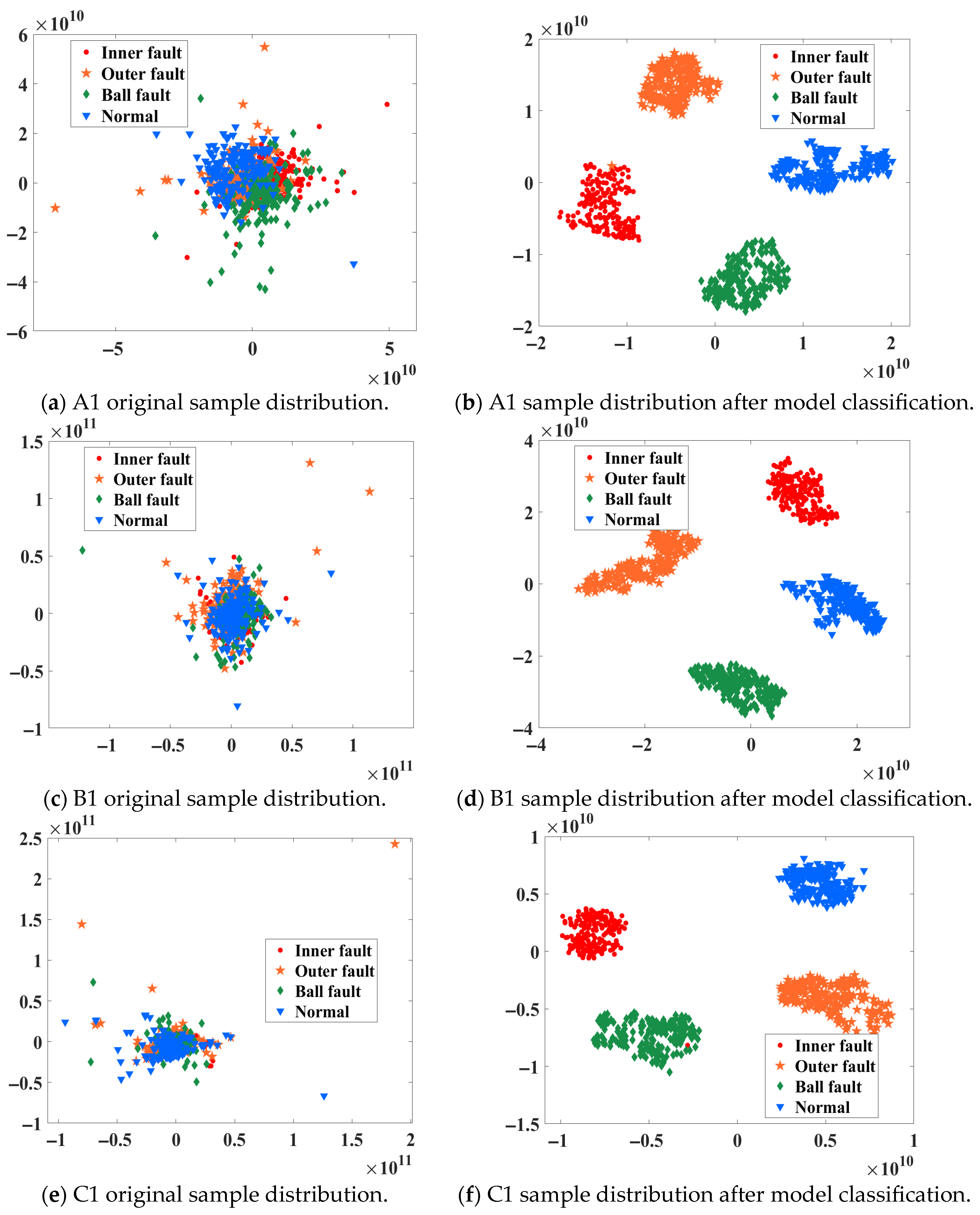
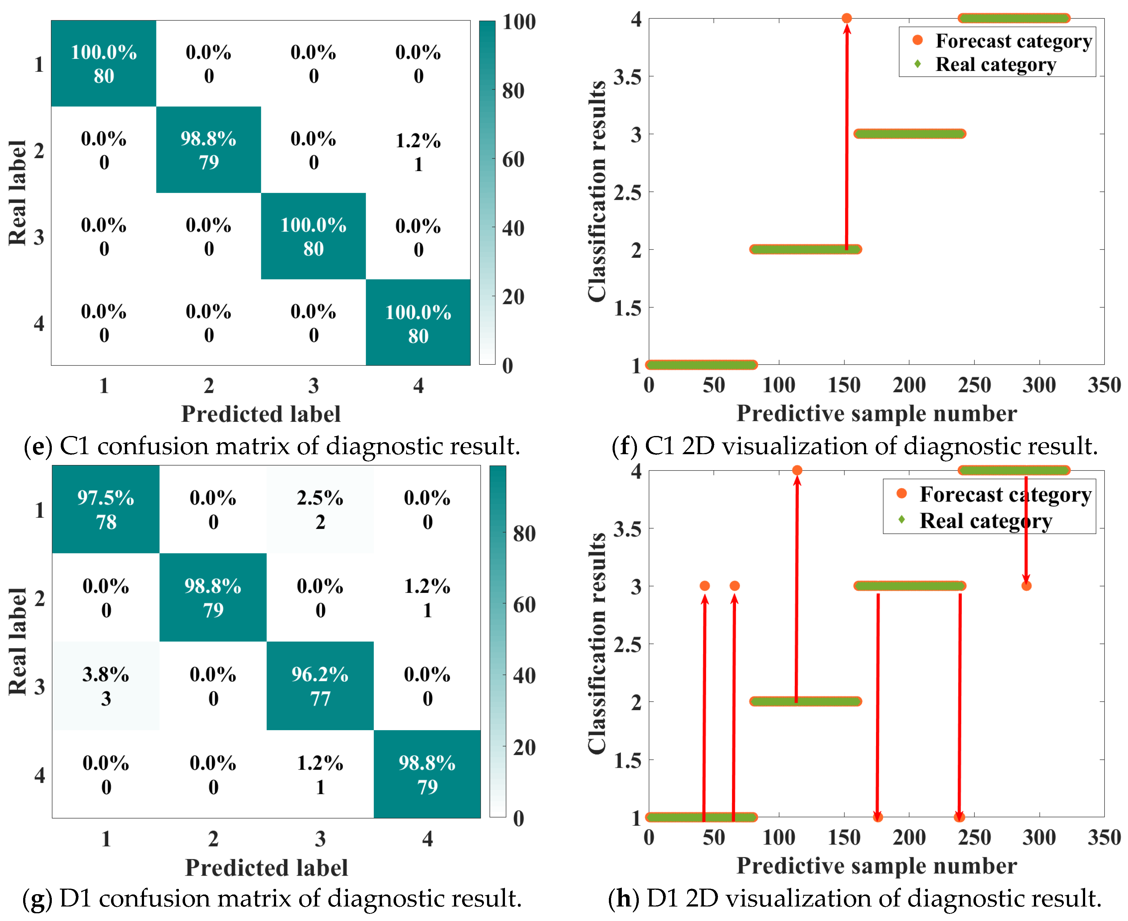
To verify the adaptability and robustness of the CNN-IPOA-LSSVM model proposed in this paper under different rotational speed conditions, experimental analyses were conducted based on the Ottawa dataset for four variable speed operating conditions (A1, B1, C1, and D1). Figure 14 and Figure 15 demonstrate the distribution of fault samples and the classification effect of the model under different speeds, and the diagnostic performance of the model under variable operating conditions is intuitively reflected by the t-SNE visualization and the confusion matrix.

The classification accuracies for distinct working conditions in the Ottawa dataset are 99.69%, 100%, 99.69%, and 97.81%, with an average accuracy of 99.30%. To better evaluate the performance of the proposed classification model, this study used essential indicators such as precision, recall, F1 score, and standard deviation (Std.). The specific expressions are as follows.

Table 6. Performance indicators of fault classification model.

Types	Precision (%)	Recall (%)	F1-Score (%)	Accuracy (%)	Std. (±%)
IF	99.72	99.68	99.70	99.69	0.12
OF	100	100	100	100	0.00
BF	99.65	99.73	99.69	99.69	0.15
Normal	99.62	99.58	99.60	97.81	0.18
Macro-average	99.75	99.75	99.75	99.30	0.11

shows the detailed performance indicator data of the model tested on the Ottawa dataset.

Precision is the proportion of correctly predicted positive examples out of all predicted positive examples.

$$\mathrm{Precision}={\displaystyle \frac{TP}{TP+FP}}$$

(31)

Recall reflects the proportion of correctly predicted positive examples out of all actual positive examples.

$$\mathrm{Recall}={\displaystyle \frac{TP}{TP+FN}}$$

(32)

The F1 score represents the harmonic mean of precision and recall.

$$\mathrm{F1-score}=2\times {\displaystyle \frac{\mathrm{Precision}\times \mathrm{Recall}}{\mathrm{Precision}+\mathrm{Recall}}}$$

(33)

The standard deviation (Std.) is calculated based on the classification results of five independent runs, reflecting model stability.

(Note: TP: true positive; FP: false positive; and FN: false negative)

Based on the data analysis above, the CNN-IPOA-LSSVM model proposed in this paper shows near-perfect classification performance across all fault categories, with an average F1 score of 99.75% and a very low standard deviation (±0.11), greatly exceeding traditional methods. Especially in outer ring fault (OF) detection, the model attains 100% precision and recall rates. Furthermore, the model proves highly stable across five independent runs, with maximum fluctuation below 0.2%, confirming the benefits of digital twin data augmentation combined with IPOA parameter optimization.

5.3. Comparative Analysis of Different Models

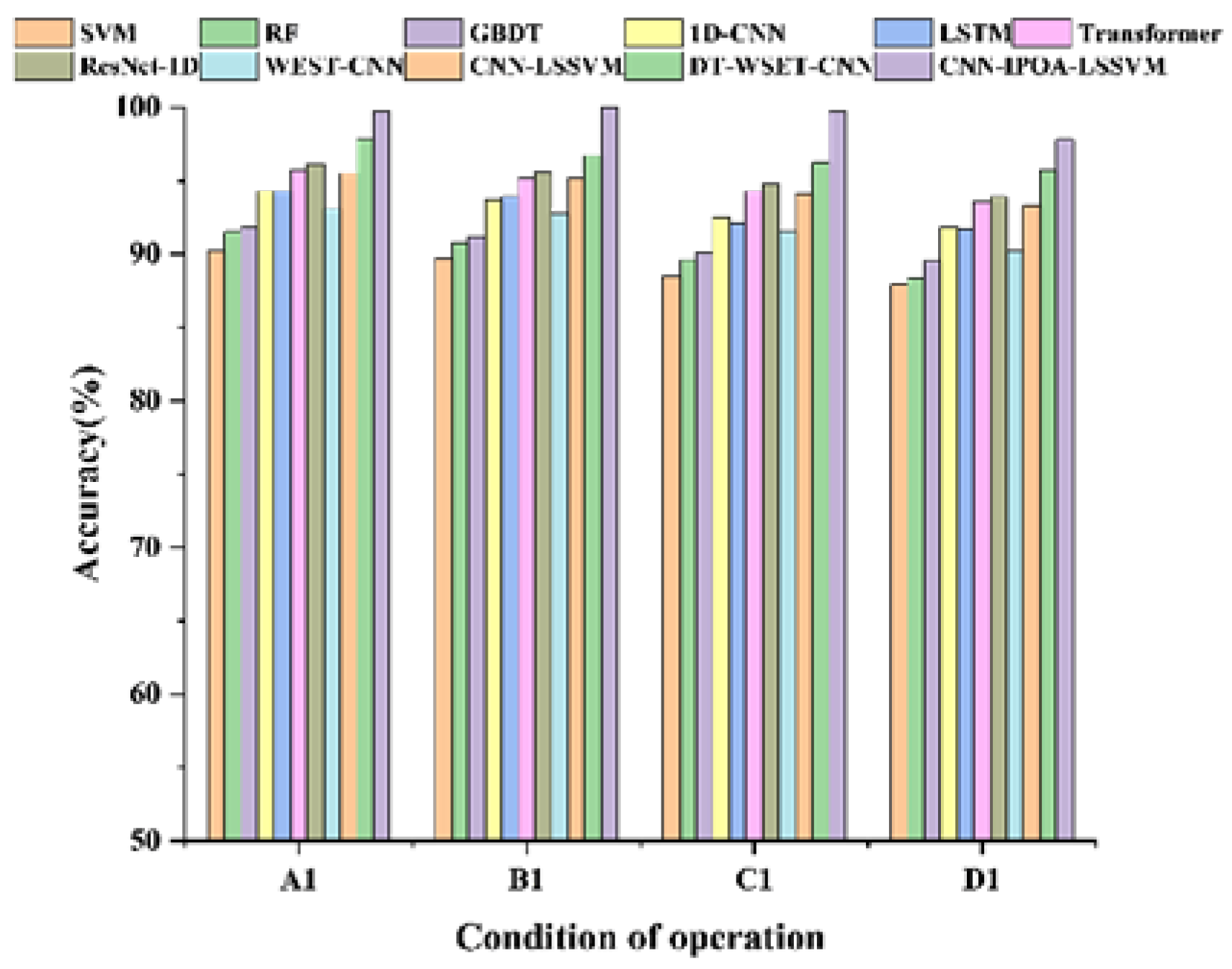
To further validate the superiority of the proposed model, the model presented in this paper is compared with several classical fault diagnosis models, including the traditional support vector machine (SVM), deep neural network (DNN), random forest (RF), one-dimensional convolutional neural network (1D-CNN), long short-term memory network (LSTM), gradient boosting tree (GBDT), one-dimensional residual network (1D-ResNet), and Transformer. Meanwhile, to verify the contributions of each module, a WSET-CNN (without digital twins), CNN-LSSVM (standard POA), and DT-WSET-CNN (without IPOA) were compared and verified. All comparison models used the same preprocessing process and the same dataset division. Model hyperparameters were optimized through grid search to ensure fairness in the comparison. The outcomes of the comparison experiments are depicted in Figure 16, and the model training curve is shown in Figure 17.

It can be seen that compared with other methods, the accuracy of the CNN-IPOA-LSSVM model proposed in this paper improves significantly compared to other diagnostic models: under the A1 growth rate working condition, it improves by 9.5%, 8.2%, and 7.9% compared to SVM (90.2%), Random Forest (91.5%), and GBDT (91.8%), respectively, and compared to the benchmark deep learning models of 1D-CNN (94.3%), LSTM (94.3%), Transformer (95.7%), and ResNet-1D (96.1%), it improves by 5.4%, 5.4%, 4% and 3.6%, respectively. Under the B1 degradation working condition, the accuracy of the model in this paper significantly outperforms that of the traditional methods (SVM 89.7%, Random Forest 90.8%, and GBDT 91.2%), with relative improvements of 10.3%, 9.2%, and 8.8%, respectively. Compared with the deep learning models, the improvements over 1D-CNN (93.7%), LSTM (93.9%), Transformer (95.2%), and ResNet-1D (95.6%) are 6.3%, 6.1%, 4.8%, and 4.4%, respectively. In the face of C1 complex working conditions, the models in this paper show stronger dynamic adaptability: 11.2%, 10.1%, and 9.6% improvement over the traditional models (SVM 88.5%, Random Forest 89.6%, and GBDT 90.1%); 11.2%, 10.1%, and 9.6% improvement over the DL models (1D-CNN 92.5%, LSTM 92.1%, Transformer 94.3%, and ResNet-1D 94.8%); and 9.6% improvement over the traditional models (1D-CNN 92.5%, LSTM 92.1%, Transformer 94.3%, and ResNet-1D 94.8%) Especially in the speed inflection interval (Epochs 40–60), the fluctuation amplitude of this paper’s model is 37.5% lower than that of ResNet-1D, indicating that its improved optimization algorithm can effectively track the variable speed characteristics. In the D1 reverse gear condition, the model’s performance in this paper exhibits the smallest degradation (only 1.8% compared with the A1 condition), whereas the comparison model shows an average degradation of 3.5%. The specific performance is as follows: 9.9%, 9.5%, and 8.3% improvement over SVM (87.9%), Random Forest (88.3%), and GBDT (89.5%); 6.0% improvement over 1D-CNN (91.8%); and 6.1%, 4.2%, and 3.9% improvement over LSTM (91.7%), Transformer (93.6%), and ResNet-1D (93.9%). In this bidirectional variable-speed scenario, the enhanced data generated by the method proposed in this paper through a digital twin encompasses a broader spectrum of speed combinations, thereby rendering the classification boundary more robust.

Comparing different optimization methods under the same model, the CNN-IPOA-LSSVM model proposed in this paper demonstrates significant advantages in four variable speed operating conditions of the Ottawa bearing dataset: Achieving accuracy rates of 99.7%, 100%, 99.7%, and 97.8%, respectively, in the A1 speed increase, B1 speed decrease, C1 increase then decrease, and D1 decrease then increase conditions, representing a 7.4% improvement over the WSET-CNN model without digital twins (average 91.9%), a 4.8% improvement over the standard POA-optimized CNN-LSSVM (average 94.5%), and a 2.5% improvement over the DT-WSET-CNN without IPOA (average 96.8%). The classification accuracy of 100% in the B1 condition validates the strong adaptability of the IPOA algorithm to sudden changes in signals. Training convergence analysis shows that the CNN-IPOA-LSSVM model in this paper achieves 96.8% validation accuracy in 50 epochs, compared to 75 epochs for the DT-WSET-CNN (without IPOA), 85 epochs for the CNN-LSSVM (standard POA), and the WSET-CNN (without digital twin), which did not fully converge even after 100 epochs. The final convergence accuracy reached 99.5%, outperforming DT-WSET-CNN (96.8%), CNN-LSSVM (95.3%), and WSET-CNN (92.7%) by 2.7, 4.2, and 6.8 percentage points, respectively, with a training–validation gap of only 0.4%.

Table 7. Significance test results of all-model comparisons.

Model	Accuracy Gain (Δ%)	t-Value	p-Value	Significance (α = 0.05)	Effect Size (Cohen’s d)
SVM	+9.47	15.32	<0.001	***	3.21
DNN	+8.20	12.87	<0.001	***	2.74
RF	+7.90	11.53	<0.001	***	2.45
GBDT	+7.80	10.91	<0.001	***	2.32
WSET-CNN	+7.80	12.45	<0.001	***	2.65
1D-CNN	+5.39	8.74	<0.001	***	1.87
LSTM	+5.39	8.62	<0.001	***	1.84
CNN-LSSVM	+5.20	8.15	<0.001	***	1.74
Transformer	+4.00	5.88	0.002	**	1.26
1D-ResNet	+3.59	5.21	0.003	**	1.11
DT-WSET-CNN	+2.50	4.32	0.005	**	0.92

Note: * indicates statistical significance, *** p < 0.001, ** p < 0.01, and * p < 0.05.

shows the results of the significance test for all models compared, using condition A1 as an example. Specifically: (1) Accuracy difference (Δ%) = average accuracy of CNN-IPOA-LSSVM-average accuracy of the comparison model. (2) Effect size: Cohen’s d > 0.8 is considered a “large effect.” (3) All p-values are corrected using the Bonferroni correction (to control for multiple testing errors).

Statistical test results confirm that the CNN-IPOA-LSSVM model demonstrates statistically significant (p < 0.01) and practically substantial (Cohen’s d > 0.9) performance advantages over 11 comparison methods (including eight benchmark models and three ablation models). In terms of module-specific analysis: Compared to the WSET-CNN model without digital twins, there was a 7.8% improvement, validating the critical role of virtual–physical data augmentation in feature extraction. Compared to the standard POA-optimized CNN-LSSVM model, it achieved a 5.2% improvement, demonstrating the value of the IPOA algorithm in three aspects: chaotic initialization, backward difference evolution, and firefly perturbation. Compared to the DT-WSET-CNN model without IPOA, it still maintained a 2.5% advantage, highlighting the synergistic gain effect between the parameter optimization module and the data augmentation module.

6. Conclusions

This paper introduces an intelligent fault diagnosis method for rolling bearings that combines digital twins and deep learning, forming a comprehensive technical chain of “data generation–feature extraction–parameter optimization–accurate diagnosis.”

Regarding data generation, based on the digital twin technology framework, a four-degree-of-freedom rolling bearing dynamic model is established to obtain mechanistic data. The denoised measured data and mechanistic data are jointly input into a GAN network for adversarial training, achieving simulation data generation through the fusion of virtual and real data, effectively overcoming the technical bottleneck of scarce fault samples in industrial scenarios.

Regarding feature extraction, a WSET-CNN collaborative analysis framework is developed, integrating the high-resolution time-frequency representation abilities of wavelet synchronous extraction transformation with the multi-level feature learning strengths of deep convolutional neural networks to precisely extract fault features across different scales from vibration signals.

Regarding model optimization, the IPOA algorithm was enhanced using chaotic initialization, backward differential evolution, and firefly perturbation mechanisms, significantly improving the optimization of LSSVM’s key parameters (regularization parameter and Gaussian kernel width). This allows the LSSVM classifier to demonstrate excellent generalization ability and nonlinear classification performance.

Through experimental validation, this method achieved an average diagnostic accuracy of 99.30% on the Ottawa variable-speed dataset, representing an improvement of 4.2–9.6 percentage points over traditional methods, while also demonstrating excellent noise robustness and operational condition adaptability. This research provides an effective technical solution for bearing fault diagnosis in complex industrial environments and has significant application value for advancing the development of intelligent equipment maintenance.

The model is suitable for fault monitoring and early warning for bearings in wind power, transportation, and mining machinery. It helps reduce maintenance costs and operational risks. However, its current performance relies on labeled data from specific bearing types, limiting broader application. Future work will improve generalization under unlabeled conditions and extend the method to other components such as gears and shafts.

References

1. Li, W.; Tan, Y.; Tao, Y.; Bai, D. Wear analysis of rolling bearing contact surfaces based on finite element method. Phys. Scr. 2023, 99, 015916. [Google Scholar] [CrossRef]
2. Roy, M. Failure analysis of bearings of aero-engine. J. Fail. Anal. Prev. 2019, 19, 1619–1629. [Google Scholar] [CrossRef]
3. Cui, L.; Li, W.; Wang, X.; Liu, D. A Novel Quantitative Diagnosis Method for Rolling Bearing Faults Based on Digital Twin Model. ISA Trans. 2024, 157, 381–391. [Google Scholar] [CrossRef]
4. Polančec, T.; Lesičar, T.; Tonković, Z.; Glodež, S. Modeling of rolling-contact fatigue pitting phenomena by phase field method. Wear 2023, 532–533, 205068. [Google Scholar] [CrossRef]
5. Peng, H.; Zhang, H.; Fan, Y.; Shangguan, L.; Yang, Y. A review of research on wind turbine bearings’ failure analysis and fault diagnosis. Lubricants 2023, 11, 14. [Google Scholar] [CrossRef]
6. Peng, B.; Bi, Y.; Xue, B.; Zhang, M.; Wan, S. A survey on fault diagnosis of rolling bearings. Algorithms 2022, 15, 347. [Google Scholar] [CrossRef]
7. Wang, Y.; Ding, X.; Zeng, Q.; Wang, L.; Shao, Y. Intelligent rolling bearing fault diagnosis via vision ConvNet. IEEE Sens. J. 2020, 21, 6600–6609. [Google Scholar] [CrossRef]
8. Wang, Y.; Li, D.; Li, L.; Sun, R.; Wang, S. A novel deep learning framework for rolling bearing fault diagnosis enhancement using VAE-augmented CNN model. Heliyon 2024, 10, 15. [Google Scholar] [CrossRef]
9. Zhang, K.; Fan, C.; Zhang, X.; Shi, H.; Li, S. A hybrid deep-learning model for fault diagnosis of rolling bearings. Meas. Sci. Technol. 2022, 33, 065103. [Google Scholar] [CrossRef]
10. Liu, Z.; Wu, L.; Zhang, K. A rolling bearing fault diagnosis method based on multi-scale feature cross-fusion attention. Bearing 2024, 12, 80–86. [Google Scholar] [CrossRef]
11. Li, C.; Yin, X.; Chen, J.; Yang, H.; Hong, L. Bearing intelligent fault diagnosis based on wavelet transform and convolutional neural network. Shock. Vib. 2020, 9, e8845. [Google Scholar] [CrossRef]
12. Immovilli, F.; Lippi, M.; Cocconcelli, M. Automated bearing fault detection via long short-term memory networks. In Proceedings of the 2019 IEEE 12th International Symposium on Diagnostics for Electrical Machines, Power Electronics and Drives (SDEMPED), Toulouse, France, 27–30 August 2019; pp. 27–30. [Google Scholar] [CrossRef]
13. Qin, Y.; Liu, H.; Wang, Y.; Mao, Y. Inverse physics–informed neural networks for digital twin–based bearing fault diagnosis under imbalanced samples. Knowl.-Based Syst. 2024, 292, 111641. [Google Scholar] [CrossRef]
14. Li, Z.; Ding, X.; Song, Z.; Wang, L.; Qin, B.; Huang, W. Digital twin-assisted dual transfer: A novel information-model adaptation method for rolling bearing fault diagnosis. Inf. Fusion 2024, 106, 102271. [Google Scholar] [CrossRef]
15. Zhang, Y.; Ji, J.; Ren, Z.; Ni, Q.; Gu, F.; Feng, K.; Yu, K.; Ge, J.; Lei, Z.; Liu, Z. Digital twin-driven partial domain adaptation network for intelligent fault diagnosis of rolling bearing. Reliab. Eng. Syst. Saf. 2023, 234, 109186. [Google Scholar] [CrossRef]
16. Li, X.; Yang, Y.; Pan, H.; Cheng, J.; Cheng, J. A novel deep stacking least squares support vector machine for rolling bearing fault diagnosis. Comput. Ind. 2019, 110, 36–47. [Google Scholar] [CrossRef]
17. Li, W.; Wang, G.-G.; Gandomi, A.H. A Survey of Learning-Based Intelligent Optimization Algorithms. Arch. Comput. Methods Eng. 2021, 28, 3781–3799. [Google Scholar] [CrossRef]
18. Chegini, S.N.; Amini, P.; Ahmadi, B.; Bagheri, A.; Amirmostofian, I. Intelligent bearing fault diagnosis using swarm decomposition method and new hybrid particle swarm optimization algorithm. Soft Comput. 2022, 26, 1475–1497. [Google Scholar] [CrossRef]
19. Tuerxun, W.; Xu, C.; Haderbieke, M.; Guo, L.; Cheng, Z. A Wind Turbine Fault Classification Model Using Broad Learning System Optimized by Improved Pelican Optimization Algorithm. Machines 2022, 10, 407. [Google Scholar] [CrossRef]
20. Sadeeq, H.T.; Abrahim, A.; Hameed, T.; Kako, N.; Mohammed, R.; Ahmed, D. An improved pelican optimization algorithm for function optimization and constrained engineering design problems. Decis. Sci. Lett. 2025, 14, 623–640. [Google Scholar] [CrossRef]
21. SeyedGarmroudi, S.; Kayakutlu, G.; Kayalica, M.O.; Çolak, Ü. Improved Pelican optimization algorithm for solving load dispatch problems. Energy 2024, 289, 129811. [Google Scholar] [CrossRef]
22. Harris, T.A.; Kotzalas, M.N. Advanced Concepts of Bearing Technology: Rolling Bearing Analysis; CRC Press: Boca Raton, FL, USA, 2006. [Google Scholar]
23. Shi, Z.; Yang, X.; Li, Y.; Yu, G. Wavelet-based synchroextracting transform: An effective TFA tool for machinery fault diagnosis. Control. Eng. Pract. 2021, 114, 104884. [Google Scholar] [CrossRef]
24. Greenacre, M.; Groenen, P.J.F.; Hastie, T.; D’eNza, A.I.; Markos, A.; Tuzhilina, E. Principal component analysis. Nat. Rev. Methods Primers 2022, 2, 100. [Google Scholar] [CrossRef]
25. Trojovský, P.; Dehghani, M. Pelican optimization algorithm: A novel nature-inspired algorithm for engineering applications. Sensors 2022, 22, 855. [Google Scholar] [CrossRef] [PubMed]
26. Kanso, A.; Smaoui, N. Logistic chaotic maps for binary numbers generations. Chaos Solitons Fractals 2009, 40, 2557–2568. [Google Scholar] [CrossRef]
27. Rahnamayan, S.; Tizhoosh, H.R.; Salama, M.M.A. Opposition-based differential evolution. IEEE Trans. Evol. Comput. 2008, 12, 64–79. [Google Scholar] [CrossRef]
28. Alhaj Omar, F.; Kulaksiz, A.A. Experimental evaluation of a hybrid global maximum power tracking algorithm based on modified firefly and perturbation and observation algorithms. Neural Comput. Appl. 2021, 33, 17185–17208. [Google Scholar] [CrossRef]
29. Li, Z.; Liu, F.; Yang, W.; Peng, S.; Zhou, J. A survey of convolutional neural networks: Analysis, applications, and prospects. IEEE Trans. Neural Netw. Learn. Syst. 2021, 33, 6999–7019. [Google Scholar] [CrossRef] [PubMed]
30. Huang, H.; Baddour, N. Bearing vibration data collected under time-varying rotational speed conditions. Data Brief 2018, 21, 1745–1749. [Google Scholar] [CrossRef]
Figure 1. Flowchart of the proposed model.
Processes 13 02779 g001
Figure 2. Dynamic model of rolling bearing.
Processes 13 02779 g002
Figure 3. Schematic diagram of localized defects.
Processes 13 02779 g003
Figure 4. Bearing vibration signal acquisition test bench.
Processes 13 02779 g004
Figure 5. Data plot of the original signal versus the noise-reduced signal.
Processes 13 02779 g005
Figure 6. Distribution difference map between real data and generated data.
Processes 13 02779 g006
Figure 7. Schematic diagram of the proposed modeling process.
Processes 13 02779 g007
Figure 8. Flowchart of the Improved Pelican Optimization Algorithm.
Processes 13 02779 g008
Figure 9. Schematic diagram of the CNN-IPOA-LSSVM.
Processes 13 02779 g009
Figure 11. t-SNE visualization of synthetic data diagnosis results.
Processes 13 02779 g011
Figure 12. Confusion matrix for diagnostic results of simulation data.
Processes 13 02779 g012
Figure 13. Test bench of Ottawa dataset.
Processes 13 02779 g013
Figure 14. Visualization of fault sample distribution t-SNE for Ottawa dataset.
Processes 13 02779 g014aProcesses 13 02779 g014b
Figure 15. Visualization of diagnostic results for the Ottawa fault dataset.
Processes 13 02779 g015aProcesses 13 02779 g015b
Figure 16. Comparison of diagnostic accuracy of different models on Ottawa dataset.
Processes 13 02779 g016
Figure 17. Training curves of different models on Ottawa dataset.
Processes 13 02779 g017