Prediction and Application of 0.2 m Resistivity Logging Curves Based on Extreme Gradient Boosting

Abstract

The G Block of Daqing Oilfield is a crucial area for sustainable development and stable production. In addressing the technical bottlenecks of high-resolution logging data interpretation for reservoir evaluation in the Block, this study proposes a resistivity curve prediction method based on machine learning algorithms. Traditional interpretation models relying on DLS logging data face two major challenges when applied to 0.2 m high-resolution logging: first, the interpreted effective thickness of the reservoir tends to be overestimated, and second, the accuracy of fluid property identification declines. Additionally, the lack of corresponding well-test data for new logging datasets further constrains the development of interpretation models. To tackle these challenges, this study employs the XGBoost algorithm to construct a high-precision resistivity prediction model. Through systematic analysis of various logging parameter combinations, the optimal feature set comprising HAC, MSFL, and GR curves was identified. Training and testing results demonstrate that the model achieves a mean absolute error (MAE) of 0.94 Ω·m and a root mean square error (RMSE) of 1.79 Ω·m in predicting resistivity. After optimization, the model’s performance improved significantly, with MAE and RMSE reduced to 0.75 Ω·m and 1.31 Ω·m, respectively. To evaluate the model’s reliability, an external validation test was conducted on Well GFX2, yielding MAE and RMSE values of 0.91 Ω·m and 1.43 Ω·m, confirming the model’s strong generalization capability. Furthermore, the RLLD-AC and RLLD-DEN crossplots constructed from the predicted results exhibit excellent fluid identification performance in practical applications, achieving an accuracy rate exceeding 89%, which aligns well with production test data. The findings of this study provide new technical support for fine reservoir characterization in the study area and offer significant practical guidance for development plan adjustments.

1. Introduction

As an indispensable key parameter in the evaluation of oil and gas reservoirs, the measurement accuracy of resistivity logging directly affects the accurate identification of reservoir fluid properties. Traditional resistivity logging technologies, limited by the physical resolution of the instruments, often fail to meet the requirements for detailed interpretation in the evaluation of thin interbedded reservoirs. Taking the Daqing Changyuan Oilfield as an example, after long-term development, the main oil layers have entered a high-water-cut stage, and the current focus for sustainable and stable production has gradually shifted to thinner, poorer-quality internal thin poor layers and external reservoirs. However, constrained by the vertical resolution of conventional logging systems, the existing interpretation methods achieve an accuracy rate of less than 70% in identifying the water-flooded status of internal thin poor layers. For the more heterogeneous external reservoirs, there is a lack of systematic and effective evaluation methods [1,2]. To overcome this technical bottleneck, the Daqing Oilfield has made significant progress in logging technology innovation in recent years. Through technological advancements, a new generation of logging tools with a vertical resolution as high as 0.2 m has been successfully developed [3,4,5]. These include high-precision density logging, natural gamma-ray spectroscopy logging, high-resolution spontaneous potential logging, and improved dual laterolog logging. These new technologies, combined with conventional microspherically focused logging, high-resolution acoustic logging, microelectrode logging, caliper measurements, and 2.5 m bottom gradient electrode array logging, form a comprehensive logging suite for the evaluation of thin interbedded reservoirs. This provides reliable technical support for the detailed characterization of thin and poor reservoirs.

In practical applications of the G block F oil formation group, researchers found that the traditional interpretation method based on the DLS logging series is no longer suitable for new high-resolution logging data. Specifically, when processing 0.2 m resolution logging data using conventional methods, not only does it lead to an overestimation of effective thickness, but more critically, it causes misjudgment of fluid properties, such as mistakenly identifying water layers as oil layers. The root cause of this issue lies in the fact that the existing interpretation standards for test wells were established based on the DLS logging series, while the resistivity curve characteristics obtained by the new logging system exhibit significant differences. To address this technical challenge, researchers first attempted traditional curve reconstruction methods. Although conventional multiple regression analysis performs well in predicting parameters such as porosity and permeability [6,7], due to the influence of multiple factors on resistivity logging responses—including formation water salinity, shale content, pore structure, etc.—simple statistical regression methods struggle to accurately reflect their complex variation patterns. The reconstruction results exhibit substantial errors and fail to meet actual production requirements.

With the rapid development of artificial intelligence technology, machine learning algorithms have demonstrated immense potential in the field of geophysical logging [8,9,10,11]. In recent years, researchers worldwide have achieved a series of innovative results in areas such as logging curve reconstruction [12,13,14], automatic lithology and facies identification [15,16], reservoir parameter prediction (e.g., porosity, permeability, saturation, and rock mechanical properties) [17,18,19,20,21,22,23], and fluid property discrimination [24,25,26]. Particularly, ensemble learning algorithms such as XGBoost have shown remarkable advantages in solving complex nonlinear problems due to their outstanding feature selection capabilities and prediction accuracy [10,18,27,28,29,30,31,32]. These technological advancements provide new solutions for high-precision resistivity curve reconstruction.

This study established a reliable prediction model for high-resolution resistivity curves using the XGBoost algorithm based on DLS well-logging series. Building upon this model and integrating well-testing data, an oil–water layer identification chart suitable for the 0.2 m logging series was developed. The research findings not only resolve the technical challenge of data continuity between legacy and modern logging series but also provide a scientific foundation for refined oilfield development decision-making.

2. Principles of the XGBoost Algorithm

Gradient boosting methods have been demonstrated to possess advantages in well logging-related scenarios [10,17,18,19,20,21,22]. Gradient boosting refers to a class of ensemble learning methods based on decision trees, typically composed of multiple decision trees as weak learners combined together. The fundamental idea of gradient boosting is to minimize the residuals of the objective function through iteration. In each iteration, the model is designed as a fitter for the residuals of the current model. The model’s residuals are then minimized using the gradient descent method. Typical gradient boosting methods include Adaboost and GBDT. Since these methods integrate decision trees as weak learners to form strong learners, they not only exhibit outstanding prediction accuracy but also inherit the excellent robustness of decision trees [33,34,35].

The XGBoost algorithm is a machine learning algorithm based on gradient boosting decision trees, falling under the category of ensemble learning. By combining multiple weak learners into a strong learner, this algorithm achieves data prediction and classification tasks, characterized by its efficiency, accuracy, and ease of tuning [36,37,38,39]. Compared to other gradient boosting methods, extreme gradient boosting introduces Lasso regularization and Ridge regularization terms into the objective function, aiming to reduce overfitting through feature selection, handling noisy data, and controlling model complexity. The specifics are as follows [36,37]:

For the objective function of gradient boosting $O^{(t)}$, there are

$$O^{(t)}={\displaystyle {\sum }_{i=1}^{n}l\left(y_i,{\widehat{y}}_i^{(t-1)}+f_t\left(x_i\right)\right)+\mathsf{\Omega }\left(f_t\right)}$$

(1)

where $l$ is the loss function, $y$ is the true value, $i$ is the number of samples, $t$ is the number of iterations, ${\widehat{y}}_i^{(t-1)}$ represents the predicted value at t − 1 iteration, $x$ is the sample, $f_t\left(x_i\right)$ is the predicted value at t iteration, and $\mathsf{\Omega }\left(f_t\right)$ is the regularization term. Unlike gradient boosting methods, XGBoost considers second-order derivatives and performs $f_t\left(x_i\right)$ second-order Taylor expansions. As follows, according to Taylor’s formula,

$$f(x+\Delta x)\cong f(x)+f^{\prime }(x)\Delta x+1/2f^{″}(x)\Delta x^2$$

(2)

Set up as follows:

$$x={\widehat{y}}_i^{\left(t-1\right)}$$

(3)

$$△x=f_t\left(x_i\right)$$

(4)

$$g_i={\mathsf{\partial }}_{{\widehat{y}}_i^{\left(t-1\right)}}l\left(y_i,{\widehat{y}}_i^{\left(t-1\right)}\right)$$

(5)

$$h_i={\mathsf{\partial }}_{{\widehat{y}}_i^{\left(t-1\right)}}^{2}l\left(y_i,{\widehat{y}}_i^{\left(t-1\right)}\right)$$

(6)

After simplification, the objective function becomes

$$O^{(t)}={\displaystyle {\sum }_{i=1}^n\left[g_i{f}_t\left(x_i\right)+\frac{1}{2}{h}_i{f}_t^2\left(x_i\right)\right]+\mathsf{\Omega }\left(f_t\right)}$$

(7)

where $g_i$ is the first-order derivative of $f_t\left(x_i\right)$, and $h_i$ is the second-order derivative of $f_t\left(x_i\right)$. The weak learner of XGBoost is a decision tree. In order to determine the optimal weak learner parameters, XGB parameterizes the $f_t\left(x_i\right)$ and $\mathsf{\Omega }\left(f_t\right)$ functions. After substituting the decision tree parameters, the objective function becomes

$$O^{(t)}={\displaystyle {\sum }_{j=1}^n\left[\left({\displaystyle {\sum }_{i\in I_j}{g}_i}\right){\omega }_j+\frac{1}{2}\left({\displaystyle {\sum }_{i\in I_j}{h}_i+\lambda }\right){\omega }_j^2\right]+\gamma T}$$

(8)

where ${\omega }_j$ represents the value of the $j$th node in the decision tree, $I_j$ is the sample set at leaf node $j$, $T$ is the number of leaf nodes, and $\gamma$ and $\lambda$ are pruning parameters used to control the complexity of the tree.

3. A 0.2 m LLD Curve Prediction Model Based on the XGBoost Algorithm

3.1. Data Normalization

This study selects logging data from Well GFX1 in the F oil formation of Block G as the foundational modeling dataset. The complete dataset from the entire well is divided into a training set and a test set, while logging data from Well GFX2 is used as an external validation set. Given that different logging curves have varying units and numerical ranges, such discrepancies may introduce bias in formation feature recognition. To address this, the raw data undergo normalization preprocessing, linearly scaling all feature values to the [0, 1] range. This standardization approach not only eliminates unit inconsistencies but also enhances the training efficiency and generalization capability of the neural network model. The formula is as follows:

$$X_N={\displaystyle \frac{X_i-X_{\min }}{X_{\max }-X_{\min }}}$$

(9)

3.2. Feature Parameter Combination

The DLS logging system, as a comprehensive suite of logging methods, integrates multiple measurement technologies, including dual laterolog (DLL), micro-spherically focused log (MSFL), compensated neutron log, density log, acoustic measurements, high-resolution acoustic logging, and natural gamma ray logging. Within this system, different measurement methods exhibit distinct vertical resolution characteristics. For instance, the HAC (High-Resolution Acoustic) log achieves a resolution of 15–30 cm, while the MSFL logging curve demonstrates superior vertical resolution, ranging from 5 to 15 cm. Given this disparity in resolution characteristics, when constructing a resistivity prediction model with a vertical resolution of 0.2 m, MSFL and HAC logging data are prioritized as key input parameters. This selection is primarily due to their enhanced vertical resolution, which effectively ensures the model’s accuracy requirements. Other curve combinations are presented in

Table 1. Logging curve combination.

Combination	HAC	MSFL	GR	CNL	DEN	LLD
1	√	√	√
2	√	√		√
3	√	√			√
4	√	√	√	√
5	√	√	√		√
6	√	√				√

.

3.3. Model Evaluation Metrics

Model evaluation metrics are used in data analysis and machine learning to assess the performance and reliability of predictive models. In this study, the Mean Absolute Error (MAE) and Mean Squared Error (MSE) are selected as evaluation criteria. The formulas are as follows [32,36,37]:

$$E_{MAE}={\displaystyle \frac{1}{n}}{\displaystyle \sum _{i=1}^n\left|y_i-\widehat{y_i}\right|}$$

(10)

$$E_{RMSE}=\sqrt{{\displaystyle \frac{1}{n}}{\displaystyle \sum _{i=1}^n{\left(\left|y_i-\widehat{y_i}\right|\right)}^2}}$$

(11)

3.4. XGBoost Hyperparameter Tuning

The key parameters of XGBoost include max_depth (controls the maximum depth of each decision tree), learning_rate (reduces the step size during updates to prevent overfitting), min_child_weight (determines the minimum sum of instance weight needed in a leaf node), subsample (controls the random sampling ratio for each tree), colsample_bylevel (governs the feature sampling ratio for splits at each tree level), and n_estimators (number of subtrees/boosting rounds).

In this study, a grid search method was employed to optimize six major hyperparameters in the XGBoost algorithm [37,38,39]. The optimization results are presented in

Table 2. XGBoost model parameter optimization range and optimal values.

Parameter	Optimal Value	Optimization Range
max_depth	4	3–10
learning_rate	0.10	[0.10, 0.20, 0.30, 0.40, 0.01, 0.02, 0.03, 0.05]
min_child_weight	2	[1, 2, 3, 4, 5, 6, 7, 8]
subsample	0.9	[0.5, 0.6, 0.7, 0.8, 0.9]
colsample_bylevel	0.9	[0.6, 0.7, 0.8, 0.9]
n_estimators	800	10–1000

.

3.5. Analysis of Model Prediction Performance

The prediction models constructed based on various parameter combinations were systematically applied to analyze the logging data from Well GFX1. The mean absolute error (MAE) and mean squared error (MSE) were used as evaluation metrics. As shown in

Table 3. Comparison of prediction results from six characteristic parameter models on the test set of Well GFX1.

Characteristic Parameter Combination	MAE	RMSE
HAC-MSFL-GR	0.94	1.79
HAC-MSFL-CNL	1.36	1.84
HAC-MSFL-DEN	1.38	1.87
HAC-MSFL-LLD	0.98	1.80
HAC-MSFL-GR-CNL	1.78	2.04
HAC-MSFL-GR-DEN	1.66	2.02

, the experimental results indicate that the HAC-MSFL-GR combined model delivered the optimal prediction performance, achieving MAE and RMSE values of 0.94 Ω·m and 1.79 Ω·m, respectively. By comparing the evaluation metrics across the models, the ranking of prediction accuracy is as follows: the HAC-MSFL-LLD combination performed second best, followed sequentially by HAC-MSFL-CNL, HAC-MSFL-DEN, HAC-MSFL-GR-DEN, and finally the HAC-MSFL-GR-CNL combination. These results confirm that different parameter combinations have a significant impact on the predictive capability of the models.

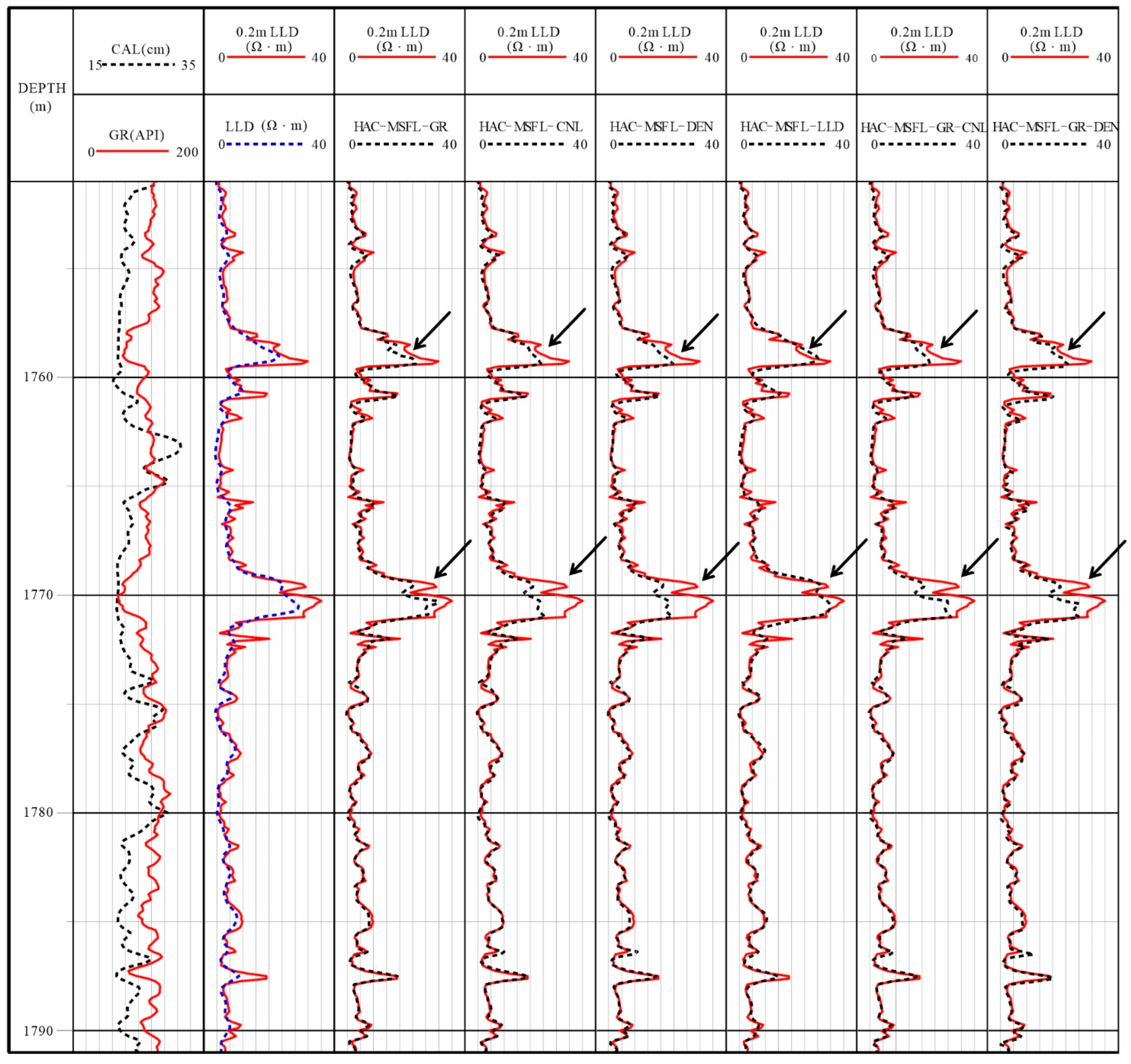
A comparative analysis between the predicted 0.2 m resistivity curves and the measured data (Figure 1 and Figure 2) reveals that all models exhibit strong agreement with the measured values in low-resistivity shale intervals. However, in thin-bedded zones, the predictions of the HAC-MSFL-LLD combination are significantly lower than the measured values, while the HAC-MSFL-CNL and HAC-MSFL-GR-CNL combinations also slightly underestimate the actual curve. The remaining three combined models demonstrate better matching accuracy (Figure 1).

For thick-bedded formations, the HAC-MSFL-LLD combination shows the best fitting performance. However, this combination suffers from a notable lack of vertical resolution, failing to effectively identify thin-bed boundaries and falling short of the 0.2 m resolution requirement. Therefore, considering both quantitative evaluation metrics, this study concludes that the HAC-MSFL-GR combination delivers the best overall predictive performance.

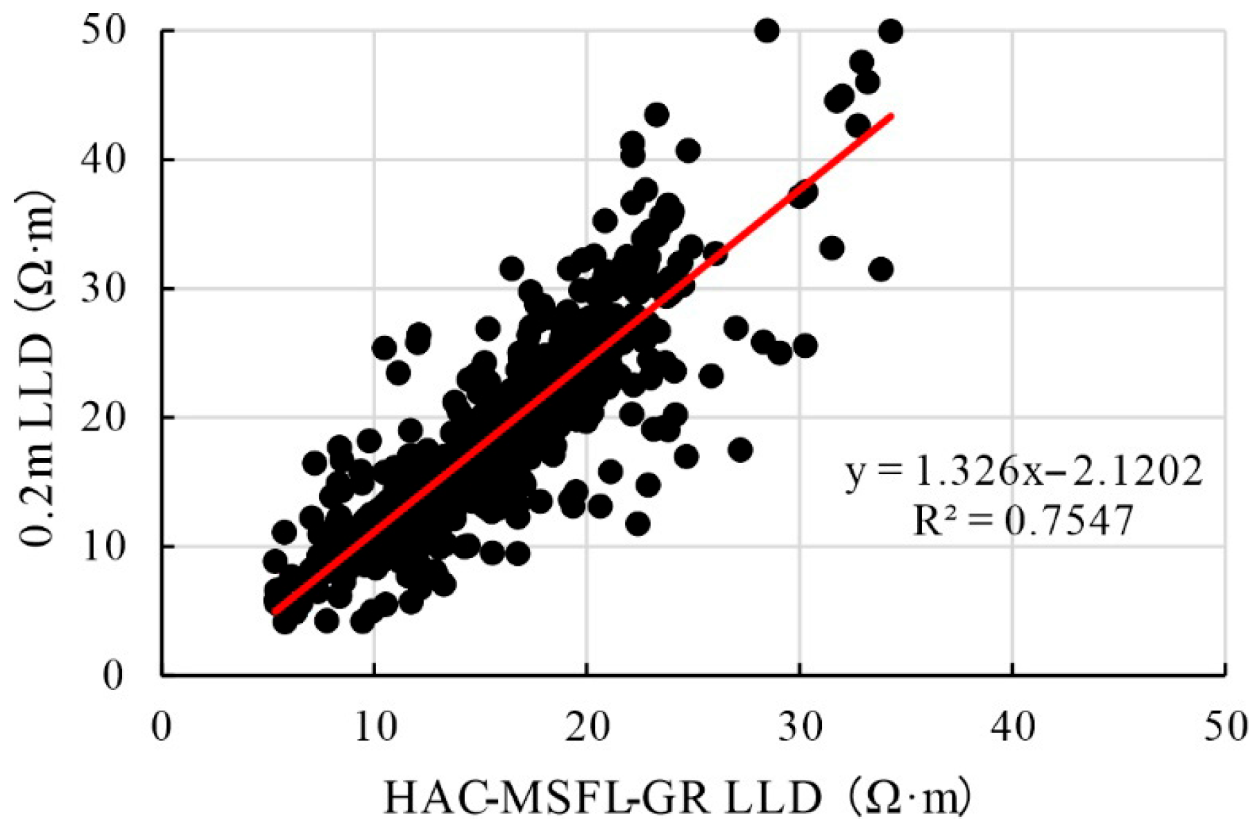
To address the systematic underestimation issue of the HAC-MSFL-GR combination in thick-bed resistivity prediction, this study implemented corrections by establishing a transformation model between predicted and measured curves. As shown in Figure 3, the correlation coefficient R² of their transformation relationship reached 0.7547. After optimizing the original predictions using this transformation, the final LLD curve prediction achieved a vertical resolution of 0.2 m, with mean absolute error (MAE) and root mean square error (RMSE) reduced to 0.75 Ω·m and 1.31 Ω·m, respectively (

Table 4. Comparison of results before and after optimization.

Characteristic Parameter Combination	MAE	RMSE
Before optimization	0.94	1.79
After optimization	0.75	1.31

), significantly improving thick-bed resistivity prediction accuracy.

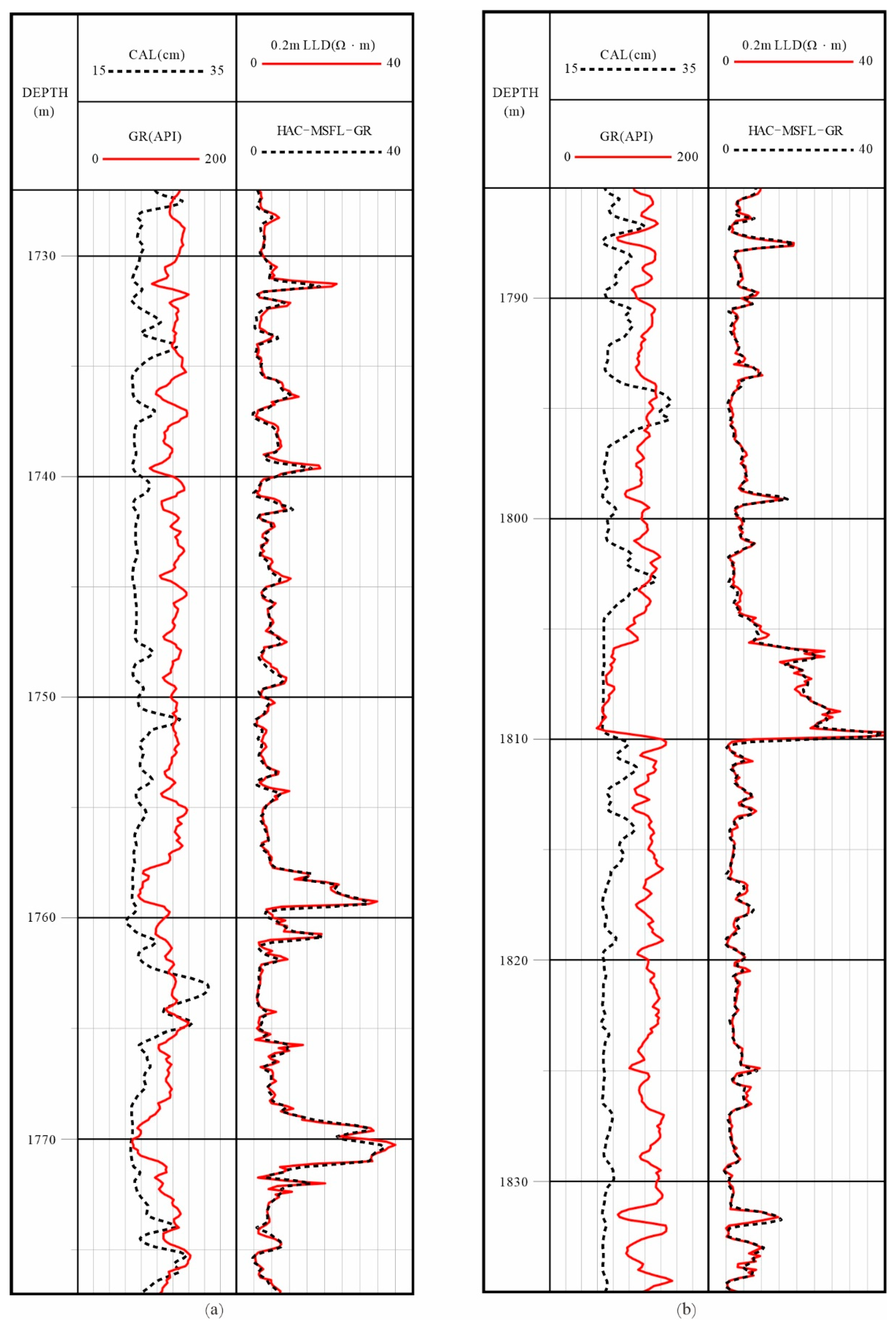
The comparative results in Figure 4 demonstrate that the optimized 0.2 m resistivity curve exhibits high consistency with the measured data in morphological characteristics. Specifically, both the magnitude and variation trends of the two curves show excellent agreement in low-resistivity shale intervals and high-resistivity sandstone layers. This fully proves that the optimized results are not only reliable but also achieve a vertical resolution comparable to the measured curve’s 0.2 m precision level.

Ultimately, an XGBoost-based logging curve prediction method was developed, which includes two key components: (1) thin-bed 0.2 m deep lateral resistivity (LLD) curve prediction using DLS logging series (HAC, MSFL and GR curves), and (2) additional correction for thick-bed 0.2 m LLD curve prediction.

3.6. Predictive Performance of HAC-MSFL-GR Combined Model on External Validation Set

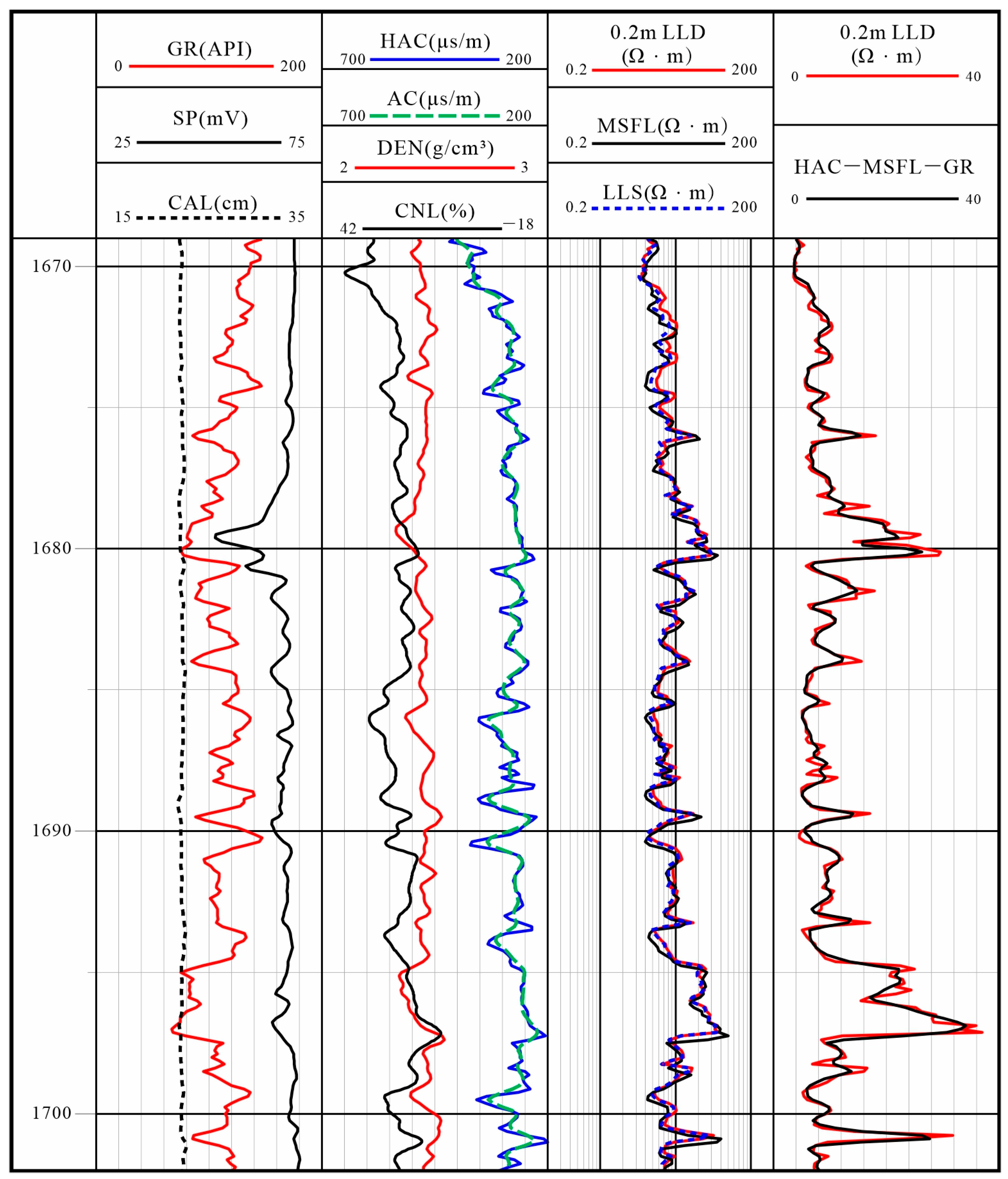
To validate the practicality and generalization capability of the developed model, this study utilized 0.2 m-resolution measured resistivity logging data from Well GFX2 in Block G as validation samples. As shown in Figure 5, the model-predicted curve demonstrates excellent agreement with the measured curve in both magnitude and morphological characteristics. Quantitative evaluation shows that the prediction results achieved MAE (Mean Absolute Error) and RMSE (Root Mean Square Error) of only 0.91 Ω·m and 1.43 Ω·m, respectively, indicating high predictive accuracy. This accuracy fully meets the precision requirements for oil–water identification chart construction, demonstrating that the proposed model possesses reliable engineering application value.

4. Discussion

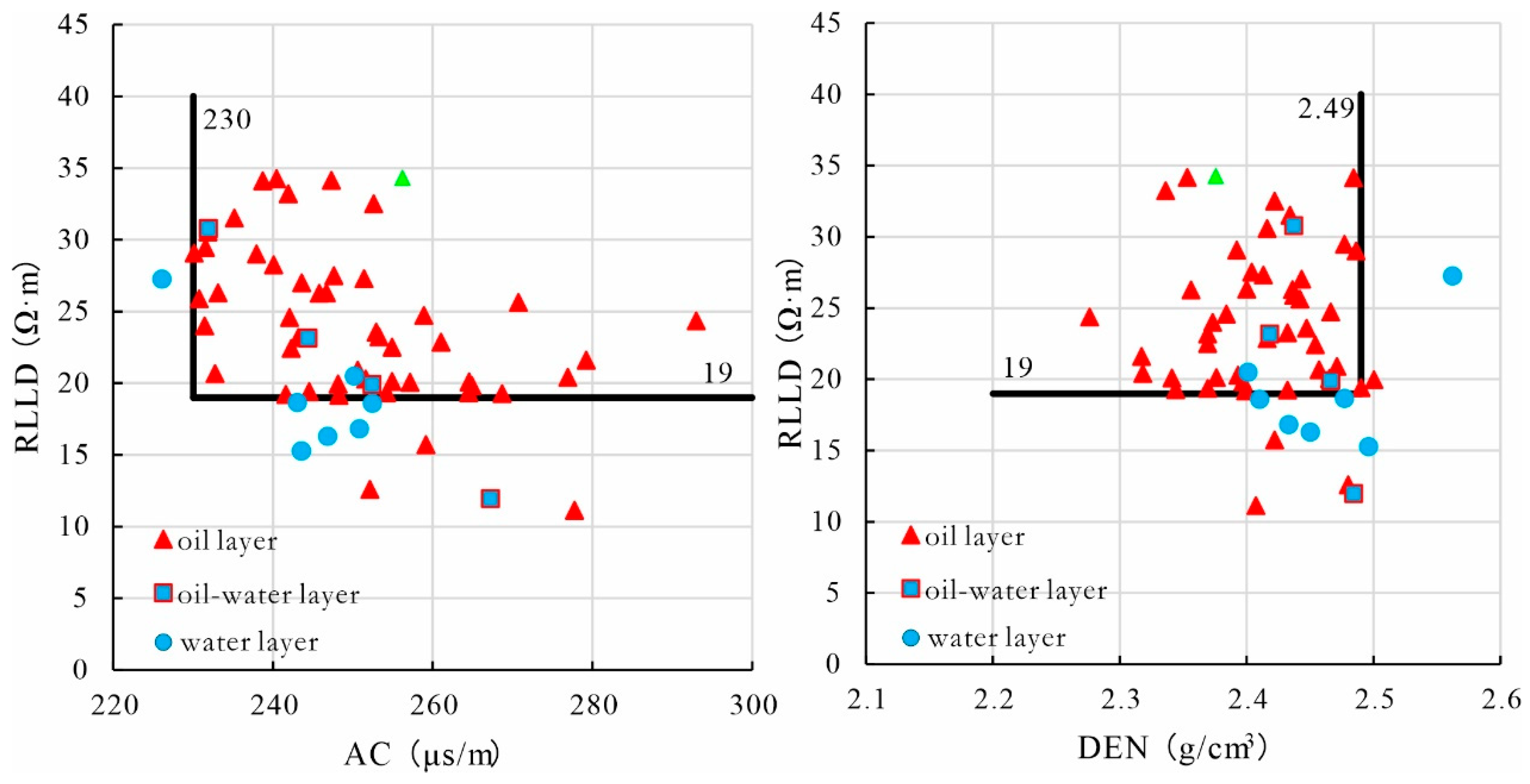
This study utilized tested well data from the DLS logging series in Block G to generate 0.2 m-resolution resistivity logging curves using the established prediction model. By integrating well testing results, key logging parameters from each tested interval were systematically extracted, including bulk density (DEN), acoustic transit time (AC), and predicted resistivity values. These parameters were employed to construct identification crossplots for oil–water zone discrimination, providing quantitative criteria for reservoir fluid characterization. Analysis of the RLLD-AC and RLLD-DEN crossplots (Figure 6) reveals that among 59 reservoir samples in the study area, 48 were oil zones, 4 were oil–water transition zones, and 7 were water zones.

For the RLLD-AC crossplot analysis:

-

Three oil zone samples were misclassified.

-

One oil–water transition zone sample was missed.

-

One water zone sample was incorrectly identified as oil.

-

Yielding an identification accuracy of 91.5%.

The RLLD-DEN crossplot results showed

-

Four oil zone samples were missed.

-

One oil–water transition zone sample was misidentified.

-

One water zone sample was falsely classified as oil.

-

With an overall accuracy of 89.8%.

Statistical analysis demonstrates that both crossplot methods achieve sufficient discrimination accuracy to meet practical oil–water identification requirements in the study area (

Table 5. Identification standards for oil and water layers in various logging series.

Logging Parameters	AC (μs/m)	DEN (g/cm3)	LLD (Ω·m)
DLS Series Standard	230	2.50	14
0.2 m Series Standard	230	2.49	19

). The identification criteria for an oil-producing zone in this formation are as follows:

When both of the following conditions are met: AC > 230 μs/m, RLLD > 19 Ω·m, or when both of the following conditions are met: DEN < 2.49 g/cm³, RLLD > 19 Ω·m. If either of the two condition sets is satisfied, the formation is identified as an oil-producing zone.

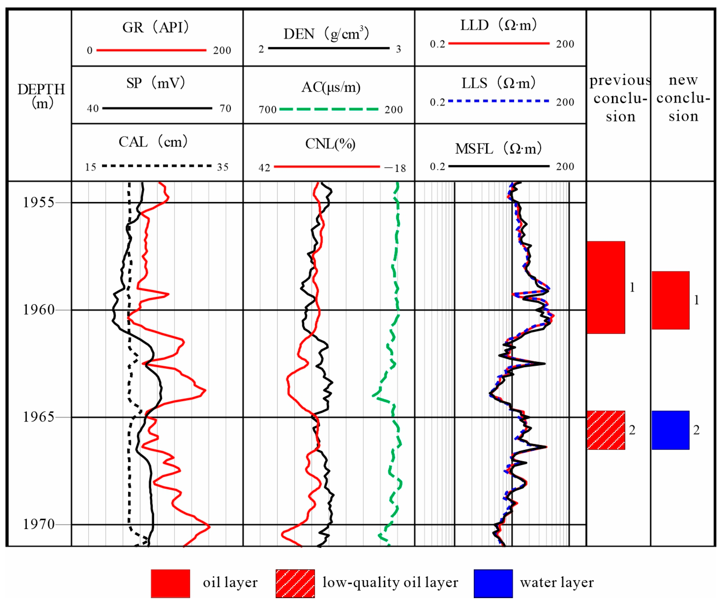
Compared with the oil–water layer evaluation criteria of the DLS logging series (Table 5), the discriminant threshold for acoustic travel time remains unchanged, while the density identification standard has been lowered by 0.01 g/cm³. These parameter adjustments have a minor impact on the net pay thickness calculation and fluid property determination. However, the changes in resistivity parameters are more significant: the resistivity threshold for DLS logging is 14 Ω·m, whereas it increases to 19 Ω·m for the 0.2 m logging series. This upward shift in the resistivity threshold will lead to a reduction in the estimated net pay thickness and raise the criteria for oil–water layer discrimination, causing some reservoirs originally classified as oil layers under the DLS standard to be reclassified as water layers. A clear demonstration of this phenomenon can be observed in the logging curve comparison in Track 3 of Figure 2—under identical formation conditions, the resistivity values (LLD) obtained from the 0.2 m logging series are significantly higher than those recorded by the DLS logging series.

4.1. Analysis of Oil Layer Identification Results

According to the DLS logging standard, Layer 1 in Well GFX3 has an effective thickness of 4.3 m, with logging parameters including an acoustic transit time (AC) of 256 μs/m, bulk density (DEN) of 2.38 g/cm³, and resistivity of 28.2 Ω·m, leading to an interpretation of it as an oil zone. In comparison, the 0.2 m logging standard defines the effective thickness as 2.7 m, with corresponding parameters of AC 254 μs/m, DEN 2.37 g/cm³, and resistivity 33.8 Ω·m (

Table 6. Logging response characteristics and comparison of production before and after fracturing.

Well No.	Layer Number	Logging Curves			Effective Thickness (m)	Pre-Frac Production			Post-Frac Production
		AC (μs/m)	DEN (g/cm3)	LLD (Ω·m)		Liquid (t)	Oil (t)	WC (%)	Liquid (t)	Oil (t)	WC (%)
GFX3	1 (DLS Series Standard)	256	2.38	28.2	4.3	6.0	0.2	96.5	15.0	2.5	83.2
	1 (0.2 m Series Standard)	254	2.37	33.8	2.7
GFX4	1	251	2.45	14.9	0.7	6.0	1.9	68.0	16.0	1.1	93.2
	2	260	2.39	18.3	1.2
	3	258	2.42	18.5	1.9

). Comprehensive analysis of the logging curves (Figure 7) and crossplot validation (Figure 8) confirm that the data points from this layer consistently fall within the oil zone range in both crossplots, further supporting the oil zone interpretation. This conclusion is consistent with the DLS logging interpretation results.

Production data from this well indicate that, prior to fracturing, the layer had a fluid production rate of 6 tons per day, with only 0.2 tons per day being crude oil and a high water cut of 96.5%. After fracturing stimulation in Layer 1, the fluid production increased to 15 tons per day, with crude oil production significantly rising to 2.5 tons per day, while the water cut decreased to 83.2%. The improvement in production performance confirms that this layer has commercial oil-producing potential. The production results effectively validate the accuracy of the well logging interpretation and further support the reliability of classifying this layer as an oil zone.

4.2. Analysis of Water Zone Identification Results

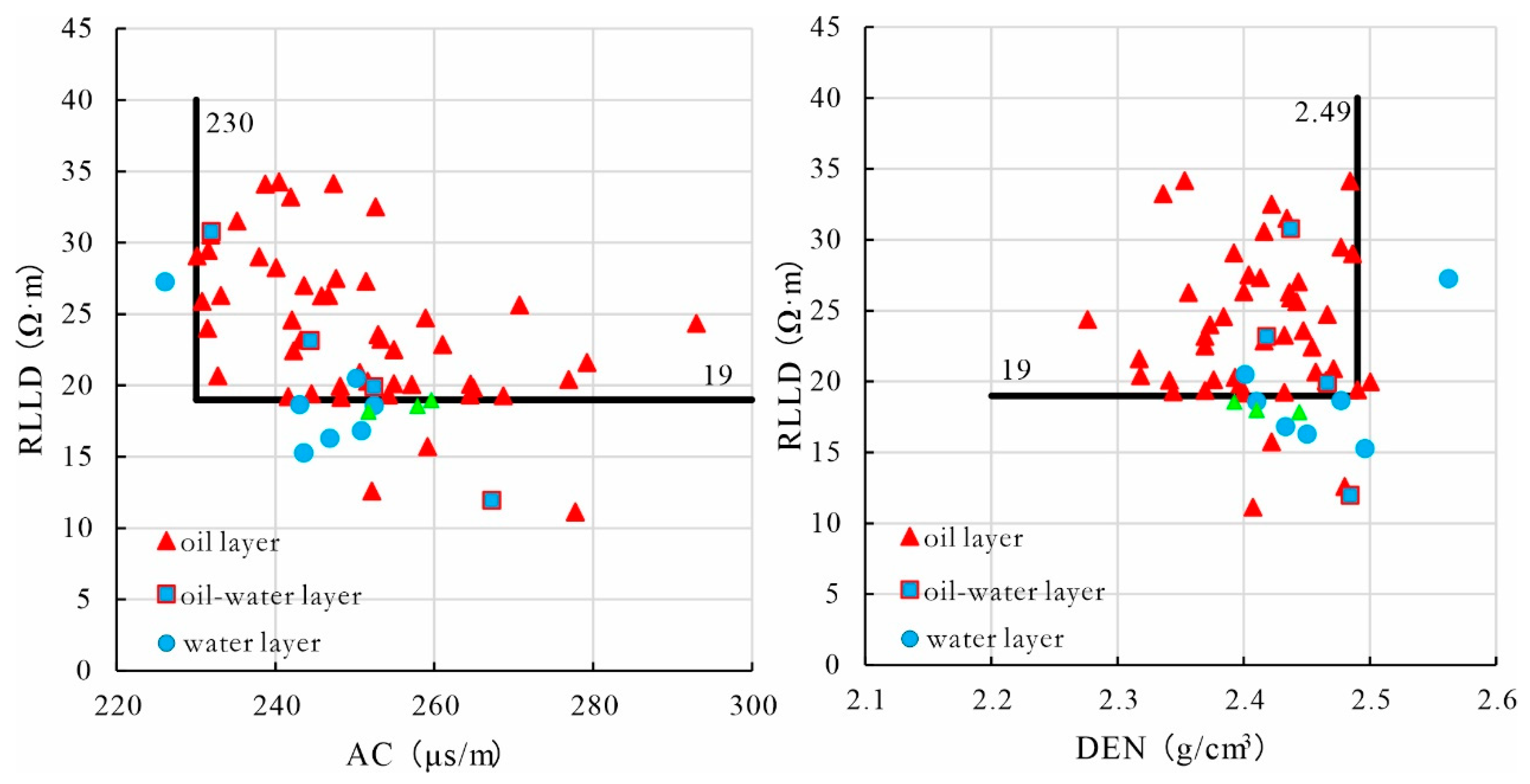
The standard interpretation results of the DLS logging series for Layers 1/2/3 of Well GFX4 indicate effective thicknesses of 0.7 m, 1.2 m, and 1.9 m, respectively, with AC values of 251/260/258 μs/m, DEN values of 2.45/2.38/2.42 g/cm³, and resistivity values of 14.9/18.3/18.5 Ω·m (Table 6), leading to an integrated interpretation of them as an oil zone (Figure 9). However, dual-plot crossplot analysis based on 0.2 m high-resolution resistivity curves reveals that these intervals exhibit distinct water zone response characteristics (green markers in Figure 10), showing significant discrepancies with the standard DLS interpretation results.

Dynamic production data provide strong support for this new understanding: prior to fracturing, the layers produced 6 tons of liquid per day (including 1.9 tons of crude oil with 68% water cut); after fracturing stimulation, while daily liquid production increased to 16 tons, crude oil production conversely decreased to 1.1 tons, accompanied by a sharp rise in water cut to over 93% (Table 6). This production behavior pattern of “increased liquid production-decreased oil production-elevated water cut” demonstrates high consistency with the development characteristics of typical water zones.

In-depth analysis indicates that the initial interpretation discrepancy primarily stems from the failure of conventional DLS logging interpretation models to adequately account for the response characteristics of 0.2 m high-resolution resistivity data. By establishing a new interpretation model, this study not only corrects previous misconceptions about reservoir fluid properties and validates the reliability of the model but more importantly provides novel technical approaches and methodological references for the interpretation of high-resolution logging data.

5. Conclusions

This study proposes a novel logging parameter prediction method based on XGBoost machine learning technology. The core innovations of this method include:

(1)

Constructing a predictive model using DLS logging data such as high-resolution array lateral (HAC), micro-spherically focused (MSFL), and natural gamma (GR) logs, with a particular focus on the accurate inversion of deep lateral resistivity in 0.2 m thin layers.

(2)

Establishing a resistivity correction model suitable for thick-layer conditions, ultimately forming a comprehensive resistivity prediction framework.

The results demonstrate that the XGBoost algorithm exhibits significant advantages in high-resolution resistivity prediction. The HAC-MSFL-GR combined model outperforms other parameter combinations in predictive performance. After thick-layer correction, the model’s overall prediction error is significantly reduced, with mean absolute error (MAE) and root mean square error (RMSE) controlled within 0.75 Ω·m and 1.31 Ω·m, respectively.

Experimental results show that the model exhibits strong generalization performance across multiple validation wells in the study area, with MAE and RMSE values of 0.91 Ω·m and 1.43 Ω·m, respectively, confirming its reliability in high-resolution resistivity prediction. The RLLD-AC and RLLD-DEN fluid identification crossplots constructed based on these predictions achieve an interpretation accuracy of over 89%. Production test data further validate the effectiveness of this method, successfully overcoming the limitations of traditional DLS logging interpretation, such as low accuracy and high misjudgment rates.

This method provides a new technical approach for the fine characterization of thin interbedded reservoirs, offering significant practical value for the development of high-water-cut oilfields. Additionally, it can be extended to high-precision logging interpretation in similar hydrocarbon reservoirs.

References

- Gao, D.; Ye, J.; Li, Q. An independent development method of low permeability oil thin layers with extreme high water cut in Changyuan Structure, Daqing oilfield. Oil Gas Geol. 2017, 38, 181–188. [Google Scholar] [CrossRef]
- Ding, J. Classifying standards of the untabulated reservoirs in Lasaxing Oilfields. Pet. Geol. Oilfield Dev. Daqing 2019, 38, 130–135. [Google Scholar] [CrossRef]
- Tong, S.; Song, J. Numeric simulation of 0.2 m vertical resolution dual laterolog tool. Prog. Geophys. 2014, 29, 2251–2257. [Google Scholar] [CrossRef]
- Tong, S.; Zhang, J.; Ding, Z. Eimulation design of dual laterolog equipment with 0.2 m high resolution. World Geol. 2020, 39, 141–149. [Google Scholar]
- Dong, J.; Miao, Q.; Liu, J. A new interpreting technique for the thin and poor untabulated water-flooded layers based on 0.2 m high-resolution logging series. Pet. Geol. Oilfield Dev. Daqing 2017, 36, 123–128. [Google Scholar] [CrossRef]
- Wang, J.; Liang, L.; Deng, Q.; Tian, P. Research and application of log reconstruction based on multiple regression model. Lithol. Reserv. 2016, 28, 113–120. [Google Scholar] [CrossRef]
- Zhu, W.; Song, T.; Wang, M.; Jin, W.; Song, H.; Yue, M. Stratigraphic subdivision-based logging curves generation using neural random forests. J. Pet. Sci. Eng. 2022, 219, 111086. [Google Scholar] [CrossRef]
- Korjani, M.; Popa, A.; Grijalva, E.; Cassidy, S.; Ershaghi, I. A New Approach to Reservoir Characterization Using Deep Learning Neural Networks; SPE: Anchorage, AK, USA, 2016; p. SPE-180359-MS. [Google Scholar] [CrossRef]
- Chen, Y.; Zhang, D. Well log generation via ensemble long short-term memory (EnLSTM) network. Geophys. Res. Lett. 2020, 47, e2020GL087685. [Google Scholar] [CrossRef]
- Sun, Y.; Zhang, J.; Zhang, Y. Adaboost algorithm combined multiple random forest models (Adaboost-RF) is employed for fluid prediction using well logging data. Phys. Fluids 2024, 36, 016602. [Google Scholar] [CrossRef]
- Chen, Y.; Zhang, D. Physics-constrained deep learning of geomechanical logs. IEEE Trans. Geosci. Remote Sens. 2020, 58, 5932–5943. [Google Scholar] [CrossRef]
- Zhai, X.; Gao, G.; Li, Y. Reconstruction method of logging curves by 2D convolutional neural network integrating attention mechanism. Oil Geophys. Prospect. 2023, 58, 1031–1041. [Google Scholar] [CrossRef]
- Wang, J.; Wen, X.; He, L. Logging curve prediction based on a CNN-GRU neural network. Geophys. Prospect. Pet. 2022, 61, 276–285. [Google Scholar] [CrossRef]
- Chen, Z.; Zhang, Y.; Li, J.; Hui, G.; Sun, Y. Artificial intelligence large model for logging curve reconstruction. Pet. Explor. Dev. 2025, 52, 744–756. [Google Scholar] [CrossRef]
- Yang, M.; Zhuang, J.; Wang, M. Leveraging Recurrent Neural Networks for Lithology Identification and Chinese Rural Landscape Planning in Sustainable Design. Sustainability 2025, 17, 3078. [Google Scholar] [CrossRef]
- Li, N.; Xu, B.; Wu, H.; Feng, Z.; Li, Y.; Wang, K.; Liu, P. Application status and prospects of artificial intelligence in well logging and formation evaluation. Acta Pet. Sin. 2021, 42, 508–522. [Google Scholar]
- Zhu, L.; Zhang, C.; Zhang, C.; Zhang, Z.; Zhou, X.; Liu, W.; Zhu, B. A new and reliable dual model and data-driven TOC prediction concept: A TOC logging evaluation method using multiple overlapping methods integrated with semi-supervised deep learning. J. Pet. Sci. Eng. 2020, 188, 106944. [Google Scholar] [CrossRef]
- Xu, B.; Tan, Y.; Sun, W.; Ma, T.; Liu, H.; Wang, D. Study on the Prediction of the Uniaxial Compressive Strength of Rock Based on the SSA-XGBoost Model. Sustainability 2023, 15, 5201. [Google Scholar] [CrossRef]
- Zhao, W.; Liu, T.; Yang, J.; Zhang, Z.; Feng, C.; Tang, J. Approaches of Combining Machine Learning with NMR-Based Pore Structure Characterization for Reservoir Evaluation. Sustainability 2024, 16, 2774. [Google Scholar] [CrossRef]
- Tang, Q.; Lu, Y.; Yang, X.; Li, Y.; Zhang, W.; Yang, Q.; Tian, Z.; Deng, R. Application of the NOA-Optimized Random Forest Algorithm to Fluid Identification—Low-Porosity and Low-Permeability Reservoirs. Processes 2025, 13, 2132. [Google Scholar] [CrossRef]
- Gohari Nezhad, A.; Emami Niri, M. Enhancing water saturation predictions from conventional well logs in a carbonate gas reservoir with a hybrid CNN-LSTM model. J. Pet. Explor. Prod. Technol. 2025, 15, 89. [Google Scholar] [CrossRef]
- Hussain, W.; Luo, M.; Ali, M. Advanced Permeability Prediction Through Two-Dimensional Geological Feature Image Extraction with CNN Regression from Well Logs Data. Math Geosci. 2025, 57, 657–702. [Google Scholar] [CrossRef]
- Tong, D.; Yuwei, L. In-Situ Stress Prediction Model for Tight Sandstone Based on XGBoost Algorithm. J. Min. Sci. 2024, 60, 341–356. [Google Scholar] [CrossRef]
- Liang, Y.; Zhang, B.; Wang, W.; Fang, S.; Zhang, Z.; Peng, L.; Zhang, Z. Deep Learning-Based Fluid Identification with Residual Vision Transformer Network (ResViTNet). Processes 2025, 13, 1707. [Google Scholar] [CrossRef]
- Hua, Y.; Gao, G.; He, D.; Wang, G.; Liu, W. Reservoir fluid identification based on multi-head attention with UMAP. Geoenergy Sci. Eng. 2024, 238, 212888. [Google Scholar] [CrossRef]
- Li, H.; Chen, M.; Zhang, X.; Yang, B.; Zhao, B.; Li, X.; Wang, H. Reservoir Fluid Identification Based on Bayesian-Optimized SVM Model. Processes 2025, 13, 369. [Google Scholar] [CrossRef]
- Liu, Z.; Wang, Z.; Zhou, D. Pore Distribution Characteristics of the Igneous Reservoirs in the Eastern Sag of the Liaohe Depression. Open Geosci. 2017, 9, 161–173. [Google Scholar] [CrossRef]
- Zhang, J.; Liu, K.; Wang, M. Downscaling Groundwater Storage Data in China to a 1-km Resolution Using Machine Learning Methods. Remote Sens. 2021, 13, 523. [Google Scholar] [CrossRef]
- Liu, Z.; Wu, H.; Zhang, S.; Zhao, X. Study on the Reservoir Heterogeneity of Different Volcanic Facies Based on Electrical Imaging Log in the Liaohe Eastern Sag. Processes 2023, 11, 2427. [Google Scholar] [CrossRef]
- Mu, Z.; Li, C.; Liu, Z.; Liu, T.; Zhang, K.; Mu, H.; Yang, Y.; Liu, L.; Huang, J.; Zhang, S. Intelligent Classification Method for Tight Sandstone Reservoir Evaluation Based on Optimized Genetic Algorithm and Extreme Gradient Boosting. Processes 2025, 13, 1379. [Google Scholar] [CrossRef]
- Liu, Z.; Wu, H.; Chen, R. Evaluation of volcanic reservoir heterogeneity in eastern sag of Liaohe Basin based on electrical image logs. J. Pet. Sci. Eng. 2022, 211, 110115. [Google Scholar] [CrossRef]
- Younes, N.; Ali, R.; Farzad, S.; Pouyan, F. Data-driven prediction of axial compression capacity of GFRP-reinforced concrete column using soft computing methods. J. Build. Eng. 2025, 101, 11831. [Google Scholar] [CrossRef]
- Li, P.; Zhang, J.-S. A New Hybrid Method for China’s Energy Supply Security Forecasting Based on ARIMA and XGBoost. Energies 2018, 11, 1687. [Google Scholar] [CrossRef]
- Ma, D.; Yang, H.; Yang, Z.; Liu, J.; Zhang, H.; Weng, C.; Lv, H.; Lv, K.; Zhou, Y.; Qin, C. An Intelligent Method for Real-Time Surface Monitoring of Rock Drillability at the Well Bottom Based on Logging and Drilling Data Fusion. Processes 2025, 13, 668. [Google Scholar] [CrossRef]
- Liu, X.; Zhang, T.; Yang, H.; Qian, S.; Dong, Z.; Li, W.; Zou, L.; Liu, Z.; Wang, Z.; Zhang, T.; et al. Explainable Machine Learning-Based Method for Fracturing Prediction of Horizontal Shale Oil Wells. Processes 2023, 11, 2520. [Google Scholar] [CrossRef]
- Chen, T.; Guestrin, C. XGBoost: A scalable tree boosting system. In Proceedings of the 22nd ACM SIGKDD International Conference on Knowledge Discovery and Data Mining, San Francisco, CA, USA, 13–17 August 2016; pp. 785–794. [Google Scholar] [CrossRef]
- Wang, F.; Hou, X. Machine learning-based prediction of physical parameters in heterogeneous carbonate reservoirs using well log data. Energy Geosci. 2025, 6, 122–134. [Google Scholar] [CrossRef]
- He, Y.; Su, H.; Zhang, C. Gel point estimation method of mixed crude oil based on ensemble machine learning model. J. China Univ. Pet. (Ed. Nat. Sci.) 2025, 49, 214–222. [Google Scholar] [CrossRef]
- Yang, Y.; Ju, B.; Lü, G. Machine learning methods for predicting CO2 solubility in hydrocarbons. Pet. Sci. 2024, 21, 3340–3349. [Google Scholar] [CrossRef]
Figure 1.
Comparison between predicted results from different combinations and measured resistivity. Track 1 displays the depth curve. Track 2 presents the natural gamma ray (GR) and caliper (CAL) curves. Track 3 compares the actual measured 0.2 m vertical resolution deep laterolog resistivity (LLD) with the DLS-series LLD curves, indicating that the 0.2 m LLD exhibits higher vertical resolution. Tracks 4 to 9 show a comparison between the XGBoost model predictions based on different logging curve combinations and the measured 0.2 m LLD, with arrows marking locations where significant discrepancies occur among the predictions from various combinations. In terms of fitting performance, the HAC-MSFL-GR combination yields the best prediction results, followed by the HAC-MSFL-GR-DEN combination.
Figure 2.
Comparison between predicted results from different combinations and measured resistivity. Track 1 displays the depth curve. Track 2 contains GR and CAL curves. Track 3 compares the measured 0.2 m LLD with the DLS-series LLD curves. Tracks 4 to 9 present a comparison between the XGBoost model predictions—based on different combinations of logging curves—and the measured 0.2 m LLD. Arrows indicate locations where significant prediction discrepancies occur among the various combinations. Based on the fitting performance, the HAC-MSFL-GR combination yields the best prediction results in thin layers, followed by the HAC-MSFL-GR-DEN combination. For thick layers, the HAC-MSFL-LLD combination performs the best, although it exhibits relatively lower resolution.
Figure 3.
Correlation plot between HAC-MSFL-GR predicted LLD and 0.2 m measured LLD.
Figure 4.
Comparative analysis of predicted LLD versus measured LLD in Well GFX1. As shown in Track 3 of Figures (a,b), the prediction results from the optimized XGBoost model based on the HAC-MSFL-GR combination exhibit strong agreement with the measured curves, both in thin and thick layers.
Figure 5.
Comparison between Predicted and Measured LLD in Well GFX2. As demonstrated in the last track, the predicted 0.2 m LLD curve shows strong agreement with the measured LLD curve across both thin and thick layers. These results indicate that the established model possesses strong generalization capability and can be further applied to predict the 0.2 m LLD curve in other wells.
Figure 6.
Oil–water layer identification crossplot.
Figure 7.
Log interpretation results of GFX3 Well.
Figure 8.
Crossplot display of Layer 1 logging data of Well GFX3. The green scatter point represents the projection results of Layer 1. Since they fall within the oil zone, this layer is interpreted as an oil-bearing formation.
Figure 9.
Log interpretation results of GFX4 Well.
Figure 10.
Crossplot display of Layer 1 logging data—Well GFX4. The green scatter points represent the projection results of Layer 1/2/3. Since they fall within the water zone, this layer is interpreted as a water-bearing formation.