1. Introduction
Welding is a fundamental technique extensively employed across manufacturing and fabrication industries for the purpose of joining metal parts. Two of the most common welding techniques are the shielded metal arc welding (SMAW) and the MIG—metal inert gas and MAG—metal active gas (MIG/MAG welding) [
1]. SMAW is a welding process that uses a coated electrode, while in MIG/MAG technique a wire is fed through a welding machine [
2]. One common difficulty of these techniques is defining the welding parameters, such as voltage, welding speed and gas flow rate. These parameters have direct influence on the welding results (appearance, strength and geometry). Typically, the welder chooses such parameters empirically, resulting in a suboptimal configuration leading to poor weld bead characteristics such as low strength, penetration and distortion [
3]. Recent studies have shown that variables such as voltage, current, wire feed speed, and shielding gas flow play a critical role in determining weld bead geometry, mechanical strength, and defect formation. For instance, Tran et al. [
4] reported that changes in voltage and travel speed significantly affect bead width and height in MIG welding. Eazhil et al. [
5] demonstrated that welding current and speed have a direct impact on angular distortion in GMAW of structural steels. Likewise, So et al. [
6] found that feed rate and thermal conditions influence bead shape and consistency in metal additive manufacturing processes. These results highlight that empirical parameter selection often leads to suboptimal welds, underscoring the need for systematic and data-driven approaches for welding process optimization.
As an alternative to the manual configuration, there has been significant research focused on the development of artificial neural networks (ANN) in the context of welding. In Wu et al.’s work [
7], a multilayer feedforward neural network was used to accurately and quickly predict welding distortion for an arbitrary welding sequence. There are also recurrent neural networks, which were used by Jaypuria et al. [
8], in a comparison with feedforward neural networks for modeling electron beam welding.
The prediction of parameters such as voltage, current, speed, and welding quality were covered by Chang et al. [
9], Lei et al. [
10], Mendonça et al. [
11] and Rong et al. [
12]. Abd Halim et al. [
13] present a study focused on resistance spot welding (RSW), a commonly used and cost-effective industrial process. This study introduced an application tool based on an open-sourced and customized ANN for practical predictions of critical welding parameters, including welding time, current, electrode force, tensile shear load bearing capacity, and weld quality classifications. Accuracy varies from 62.5% to 93.67% depending on the optimization parameters adopted. In Kshirsagar et al. [
14], a two-stage algorithm, consisting of a support vector machine (SVM) and ANN was adopted, considering tungsten inert gas (TIG) welding with a small dataset. The results were interesting because they improved the accuracy of the prediction of bead geometry compared to the traditional ANN method. Li et al. [
15] predicted the bead width and reinforcement using the welding speed as the variable input parameter in a GMAW process, while the other welding parameters remained constant. The adopted ANN was composed of a basic three-layer backpropagation. The input layer was the spatial welding speed sequence with 33 neurons. The accuracy on the training set was 99% and on the validation set was 96%. Xue et al. [
16] used a backpropagation ANN with a genetic algorithm to achieve the prediction of two bead geometry parameters. The author achieved an error of 5.5%. Wang et al. [
17] developed an ANN model to predict bead width, height, and contact angle in CMT-based WAAM using wire feed speed, travel speed, and interlayer temperature as inputs, achieving prediction errors below 5.1% through a combined model approach integrating geometric analysis.
Recent investigations have demonstrated the effectiveness of artificial neural networks (ANNs) and deep learning techniques in the prediction of welding outcomes, even under conditions of limited or complex datasets. Tran et al. [
4] proposed a feedforward ANN trained via backpropagation to predict weld bead geometry, using input parameters such as voltage, current, and welding speed. The model achieved mean absolute errors below 0.05 mm for bead width and height, indicating high predictive accuracy. In the context of additive manufacturing, So et al. [
6] developed a deep neural network model to predict bead geometry based on process layer data, reporting a coefficient of determination (R
2) greater than 0.97. Eazhil et al. [
5] utilized a multilayer perceptron (MLP) architecture to estimate angular distortion in gas metal arc welding (GMAW) of structural steel plates, incorporating variables such as plate thickness, current, and welding speed. The model demonstrated prediction accuracy exceeding 90%.
For classification tasks, Say et al. [
18] employed a convolutional neural network (CNN) trained on augmented datasets of X-ray images to categorize multiple classes of welding defects. The methodology, which included data augmentation and deep feature extraction, resulted in classification accuracy above 94%. Similarly, Kim et al. [
19] applied a CNN to classify penetration conditions in GMAW processes, using input data transformed through Short-Time Fourier Transform (STFT) to generate spectrograms from welding signals. The proposed model achieved classification accuracy over 95%. Collectively, these studies underscore the potential of ANN-based approaches for predictive modeling and quality assessment in welding processes, supporting the present study’s objective of optimizing neural network performance in scenarios with reduced datasets.
Each of these articles has unique architectural features that make them suitable for specific applications [
20]. However, most of the works do not apply a methodology to achieve ANN architecture parameters, meaning that the ANN architecture was defined through trial and error [
21]. The importance of optimizing welding parameters cannot be overlooked. It not only boosts the efficiency and precision of welding but also guarantees the long-term durability and structural integrity of the end product [
22]. The term artificial neural network (ANN) is used in a general sense, whereas multilayer perceptron (MLP) refers to a specific type of feedforward neural network (FNN) that includes one or more hidden layers. Throughout this study, the term artificial neural network (ANN) refers specifically to a multilayer perceptron (MLP) with a feedforward architecture.
In other contexts, there are different works focused on optimizing the architecture of neural networks. For instance, the work by Ukaoha and Igodan [
23] optimized the parameters of a deep neural network through a genetic algorithm (GA) in a binary classification application for admission of students at an university. Also using GA, Cicek and Ozturk [
24] optimized the number of neurons, hidden layers, and weights for forecasting time series considering experimental data. In other work, by optimizing the weights and numbers of hidden layers of a backpropagation ANN, Jiang et al. [
25] were able to predict investment risk problems in the electricity grid through GA. Feedforward Neural Networks (FNNs) are used in Jian-Wei’s work [
26], inspired by the optimization of a shoal of artificial fish, called artificial fish swarm optimization (AFSO), to obtain the number of hidden layers trained to replace backpropagation in ANNs. In the study of Sheng et al. [
27], an adaptive memetic algorithm is used with a classification-based mutation, named adaptive memetic algorithm with a rank-based mutation (AMARM), to optimize ANN architectures by fine-tuning connection weights between neurons as well as hidden layers. Optimization of activation functions is not as common as it is for the number of layers, neurons, and weights, in addition to the learning rate [
28].
Ilonen et al. [
29] explore the applicability of differential evolution (DE) as a global optimization method for training feed-forward neural networks. While it does not show distinct advantages in learning rate or solution quality compared to gradient-based methods, it proves valuable for validating optima and contributing to the development of regularization terms and unconventional transfer functions without gradient dependence. Slowik and Bialko [
30] present the utilization of the DE algorithm in training ANNs. The proposed approach is applied to train ANNs for classifying the parity-p problem. Comparative results with alternative evolutionary and gradient training methods, such as error back-propagation and the Levenberg–Marquardt method, highlight the potential of the differential evolution algorithm as an alternative for training artificial neural networks. Movassagh et al. [
31] contributes by focusing on the utilization of ANN and DE, for enhancing precision in prediction models. The study introduces an integrated algorithm for training neural networks using meta-heuristic approaches, emphasizing the determination of neural network input coefficients. Comparative analysis with other algorithms, including ant colony and invasive weed optimization, demonstrates superior convergence and reduced prediction error with the proposed algorithm, highlighting its effectiveness in improving perceptron neural network performance.
Through research on the application of Differential Evolution (DE) in welding optimization, several relevant studies were identified. Panda et al. [
32] proposed a method that combines neural networks with DE to optimize welding parameters, successfully improving joint strength and reducing power consumption while modeling the relationship between welding factors such as current, force, time, and sheet thickness. Similarly, Alkayem et al. [
33] used artificial neural networks (ANN) to predict weld quality based on multiple parameters and applied evolutionary algorithms like DE to optimize outputs such as tensile strength and hardness, with the Neuro-DEMO algorithm delivering superior results. Expanding on this, Alkayem et al. [
34] explored neuro-evolutionary algorithms for friction stir welding (FSW), where ANN models were coupled with multiobjective DE and particle swarm optimization (PSO) to enhance weld qualities, identifying PSO as the most efficient. The key distinction of this work lies in its focus on optimizing welding parameters specifically for gas metal arc welding (GMAW), targeting not only joint strength but also the development of a practical application to assist welders in the field, which has not been explored in previous studies.
The existing academic gap addressed by this study lies in the optimization of ANN architecture for welding parameter prediction, where configuring settings is challenging for field welders. The proposed integration of DE, cross-validation techniques, and data augmentation methods contributes to bridging this gap by offering a more effective and precise approach to derive welding parameters from specified bead geometry. The study specifically focuses on MAG welding on SAE 1020 steel, providing valuable insights into improving ANN performance in a practical and industrially relevant context. In this work, the ANN model is trained to predict welding process parameters such as voltage, gas flow rate, wire feed speed, and stickout—which are the output response indicators, based on a set of input geometric features that describe the desired weld bead: plate thickness, bevel type, root gap, weld width, and weld height. Therefore, the motivation behind this work is to optimize the parameters of an Artificial Neural Network (ANN) to accurately predict the ideal setup for MAG welding based on the required weld geometry. The novelty lies in the use of Differential Evolution (DE) optimization algorithms to enhance the accuracy of parameter prediction, as well as addressing the challenge of limited data by employing data augmentation techniques and Leave-One-Out (LOO) cross-validation. Additionally, to ensure robust benchmarking, K-Nearest Neighbors (KNN) and Support Vector Machine (SVM) models were also implemented for comparison, as these techniques are known for their effectiveness in small dataset scenarios. This research aims to develop an application that assists welders in the field by providing real-time recommendations, improving efficiency and weld quality, while reducing trial and error and minimizing production downtime.
The primary motivation for this research lies in the challenge of accurately predicting welding parameters in MAG processes using limited experimental data. This study proposes a novel integration of ANN architecture optimization with DE and SHGO, combined with LOO cross-validation and synthetic data augmentation. Additionally, we introduce KNN and SVM as comparative benchmarks, improving robustness and relevance. These contributions aim to enhance predictive reliability in small-data industrial contexts, offering practical solutions for field welding applications.
As in [
21], the present work investigates a methodology for optimally choosing the ANN architecture and parameters during training in the context of welding. However, here, DE is employed and more parameters of welding inputs and outputs are investigated. The welding inputs (voltage, speed, gas flow rate, and stickout) are predicted from a definition of bead geometry by the welding operator. In addition, to address the small dataset problem, a comparison between data augmentation techniques is carried out. The present work also aims to develop a methodology for an application to help the welder. This work also focuses on producing a dataset of welding with randomly chosen parameters to reach a wider dataset while in [
21] employs Box–Behnken design within a design of experiments (DOE) framework.
The main contributions of this work are:
A DE-optimized ANN architecture for inverse prediction of MAG welding parameters.
A comparative analysis with KNN and SVM in small dataset conditions.
Integration of data augmentation and LOO cross-validation to enhance performance.
Python-based (version 3.13.7 on Google Colab) implementation with low-cost deployment potential.
The structure of this paper is as follows:
Section 2 reviews related work on welding parameter prediction using AI techniques.
Section 3 presents the methodology, including dataset preparation, model design, and optimization.
Section 4 discusses the results, followed by benchmarking and validation. Finally,
Section 5 concludes with future work and limitations.
2. Optimization
The ANN architecture can be optimized and thus resulting in the best setting for predicting welding parameters that result in more standardized welds. In the present work, the focus was directed to the differential evolution (DE), which is an optimization technique initially presented in 1996 by Storn and Price with characteristics of easy implementation, fast convergence, and few parameter settings for initialization [
35]. DE is inspired by mechanisms of natural selection and genetics of populations of living beings, with mutation, crossing and selection operators to generate new individuals from a population in search of the most adapted.
In this numerical approach, some parameters must be defined [
36]. The population size (NP) determines the number of candidate solutions or individuals in each generation. A larger NP can increase exploration but may also lead to increased computational costs. The mutation scaling factor (F) controls the amplification of the difference between two randomly selected individuals in the population to create a new trial solution. It plays a crucial role in balancing exploration and exploitation. Crossover probability (CR) dictates the probability of incorporating the trial solution into the next generation. A higher CR value promotes greater exploration, while a lower value encourages exploitation. In addition, a stopping criterion must be chosen. The common choices include the maximum number of iterations (generations), a target fitness value, or a convergence threshold. The maximum number of iterations is the stopping criterion considered to finalize the evolutionary process or a convergence threshold. Finally, the objective function quantifies the quality of a solution and depends on the problem being optimized [
35]. A flowchart of a DE algorithm typically illustrates the sequence of steps involved in its operation, as shown in
Figure 1.
During the initialization, a population of candidate solutions is created randomly within predefined bounds and F and CR. The values chosen for CR and F in the initial population of DE impact the balance between exploration and exploitation. The generation counter is set at t = 0. The Mutation operation involves selecting three distinct individuals in the population and computing a mutant vector, with the scaling factor F. In crossover, a random vector with the proper dimension is generated and compared to CR. This comparison is employed to recombine the original solution with the mutant vector. Selection compares the trial solution’s fitness with the original solution’s fitness. If the trial solution is better (or equal), it replaces the original solution in the next generation. These steps are repeated sequentially until the algorithm terminates when the termination criterion is satisfied [
35,
37].
Although DE is a well-established optimization method, its application remains relevant for scenarios involving limited data availability, particularly when combined with data augmentation techniques such as kriging and SDV. This approach provides a practical and computationally efficient alternative to deep learning models that typically require larger datasets. The DE algorithm offers advantages such as simplicity, robustness against local minima, and effective global search capabilities, making it well-suited for neural network optimization [
38,
39].
Another optimization technique is the simplicial homology global optimization (SHGO), which is a technique that combines concepts from simplicial homology theory with local search methods to find the global minimum of a function in a multidimensional space. The SHGO is based on the construction of simplicial complexes in the search space, which are structures formed by combinations of points and their interconnections. These complexes capture information about the topology of the search space and allow exploring its structure efficiently [
40,
41].
As aforementioned, herein both DE and SHGO will be employed for optimizing the architecture of an ANN for defining welding parameters for chosen welding characteristics. For this purpose, an experimental dataset was generated. As this dataset is small, techniques for data augmentation were explored. These techniques are described in the next section.
4. Methodology
In this study, bead geometry was selected as the target response for inverse prediction of MAG welding parameters due to its direct association with weld quality, dimensional accuracy, and mechanical performance, which are critical in industrial fabrication processes. Bead height and width, in particular, are measurable outcomes that reflect the effectiveness of the welding parameters and are often prioritized in quality inspections. The selected output variables—voltage, wire feed speed, gas flow rate, and stickout—were chosen based on their high practical relevance and controllability during the welding process. These parameters are directly adjusted by operators and have a well-documented influence on arc stability, heat input, and material deposition, as supported by studies such as Wang et al. [
17], Li et al. [
15] and Eazhil et al. [
5]. Furthermore, the use of Differential Evolution (DE) and Simplicial Homology Global Optimization (SHGO) to optimize the ANN architecture was motivated by their proven ability to handle complex, non-convex search spaces with small datasets. The parameter ranges for optimization were defined based on observed industrial practices, welding standards, and experimental constraints to ensure the model’s applicability in real-world scenarios. This methodological framework allows the model to provide precise and usable welding settings from geometrical bead characteristics, even when trained on limited data enhanced through structured data augmentation techniques.
Artificial neural networks (ANNs) were selected as the primary modeling technique in this study due to their ability to capture complex, non-linear relationships between multiple variables, which is critical in the context of inverse welding parameter prediction. While traditional machine learning models such as K-nearest neighbors (KNN) and support vector machines (SVM) are often recommended for small datasets due to their proven effectiveness, in this study, they were primarily calculated for comparative purposes to evaluate the relative performance of different approaches. The focus on ANN architecture optimization through evolutionary algorithms, such as Differential Evolution, aims to enhance predictive performance by tailoring the model structure to the specific challenges of the welding domain. This strategy aligns with the study’s objective of developing a flexible, accurate model for real-world application in MAG welding.
4.1. Dataset
The research problem addressed in this work involves identifying the optimal architecture of an artificial neural network (ANN) to define the MAG welding parameters for a specific geometry. It is important to note that the trial-and-error approach is still commonly used in many cases within the welding context for defining such architectures. This study presents an alternative method aimed at mitigating this issue. To create the dataset, MAG welding experiments were conducted following the manufacturing characteristics outlined in
Table 1.
SAE 1020 is a low-carbon steel with good weldability and a large range of applications in industry. AWS ER70S6 wire is designed for welding mild and low alloy steels, making it a suitable match for SAE 1020. The steel plates were cut through a guillotine, with the type of bevel being machined.
Figure 2 shows the fixing of the plates in addition to the sample’s dimensions. In (a), the fixing and root spacing template of the steel plates is shown. In (b), the V bevel is shown, in (c) there are the measurements used in the samples, while in (d) and (e) there are two welded specimens. Root gap, sheet height, and thickness vary in the range displayed in
Figure 2.
The composition of the SAE 1020 steel and its equivalent carbon (
) are given in
Table 2.
For welding SAE 1020 steel plates with thicknesses between 1/8″ and 1/4″ inch (around 3 to 6 mm), preheating is generally not necessary if the
is low, as in the case with a
of 0.27. According to welding guidelines, steels with a
below 0.40 typically do not require preheating unless specific conditions, like highly restrained joints or cold working environments, are present [
62].
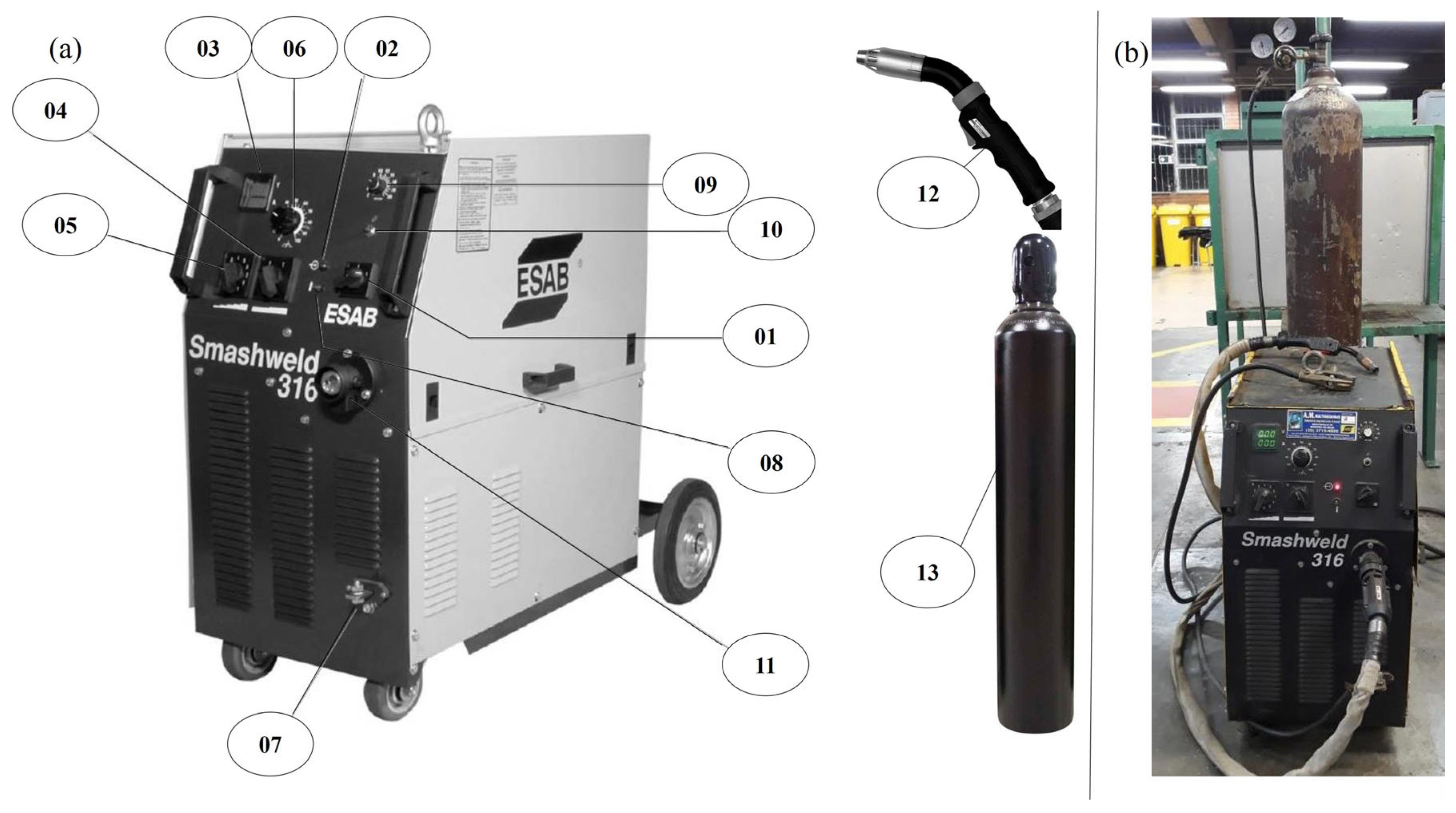
The welding equipment functions are described in
Figure 3a with following description of the setup configurations in
Table 3 and the real equipment is presented in
Figure 3b.
The selection of specific parameters such as voltage, current, gas flow, feed speed, and stickout is driven by their critical impact on the quality and consistency of the welding process. Voltage and gas flow directly influence arc stability and weld penetration, while feed speed controls the rate at which filler material is deposited, affecting bead formation. Stickout affects current transfer and heat concentration in the weld. These factors must be precisely adjusted to achieve the desired bead geometry, which is defined by plate thickness, bevel type, gap, height, and width. For welding on SAE 1020 steel using the MAG process, these input parameters are essential for ensuring structural integrity and meeting the required specifications.
In the experiments, the parameters were randomly set during the welding of the test specimens, meaning they were adjusted manually on the machine, which could result in weld beads with irregular geometry. These parameters were adjusted for the subsequent training of the neural network. With the results obtained for the width and height of the weld bead for SAE 1020, it was possible to tabulate and organize the data in
Table 4 for further analysis. The number of passes for the steel plates of 3.18 mm and 4.76 mm is 1, for the 6.3 mm is 2 and for the 9.52 mm is 3.
Table 4 presents the considered input and output data for developing the ANN in this work. Note that the inputs refer to the characteristics of the joint (sheet thickness, bevel type, root opening, bead height and bead width), while the outputs are welding parameters (gas flow, voltage, wire feed speed and stickout). The idea is that the welder specifies the desired characteristics of the joint and the ANN selects a proper set of welding parameters.
To contextualize the optimization strategy adopted in this study,
Table 5 summarizes the main trends in neural network topology optimization. It includes commonly addressed elements such as the number of layers and neurons, activation function selection, hyperparameter tuning, and data augmentation. Typical techniques associated with each trend are listed, along with their respective application (or non-application) in the present work. This table not only reinforces the relevance of using Differential Evolution (DE) for optimizing architectural and learning parameters but also clarifies the methodological decisions regarding the exclusion of pruning techniques and the benchmarking against other machine learning models. It serves as a structured overview of the optimization framework and its alignment with current best practices in ANN-based predictive modeling.
It is worth mentioning that, during the dataset development, the welder set these parameters and then measured the dimensions. Therefore, this relationship is only valid for the process and material specified. The geometrical welding parameters from the inputs are shown in
Figure 4 with the welded zone in black.
The experimental values used for ANN inputs and outputs are presented in
Table 4. These values compose the experimentally generated dataset, which will be adopted for developing the ANN.
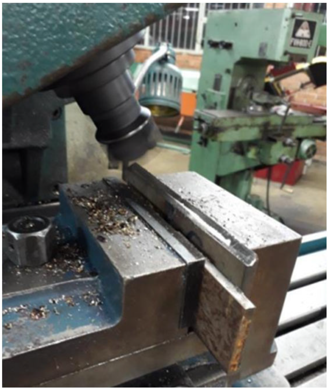
The samples were cut using a Cruanes TM10 (Selmach Machinery, Hereford, UK) guillotine shear, and the bevels were created using a Kone KFU2 (Limeira, Brazil) universal milling machine.
Figure 5 illustrates the beveling machining process.
The values for the height and width of the weld beads were measured using a digital caliper (with centesimal resolution). The decision to use a digital caliper with a centesimal resolution of 0.01 mm for measuring the height and width of the weld beads is justified by the need for high precision in capturing the geometric details of the welds. Given that small variations in bead geometry can significantly impact the quality and structural integrity of the weld, accurate measurements are essential. A resolution of 0.01 mm ensures that even minor deviations in weld bead dimensions are detected, providing reliable data for training the neural network. This level of precision is particularly appropriate for this study, where the geometry of the weld plays a critical role in optimizing the welding process. The root gap was ensured with the placement of a standard piece between the specimens as shown in
Figure 2a.
4.2. Data Processing and Augmentation
As can be seen in
Appendix A, this database is composed of only 44 pairs of input-output data. In order to augment the dataset, Kriging and SDV techniques were used to increase the dataset size to 50% (condition 1.5), 100% (condition 2.0), and 150% (condition 2.5), as shown in
Table 6. Based on the tests carried out on an ANN (which will be discussed below), the errors presented were compared and the technique with the best performance was chosen for optimization. The Sklearn library and GaussianProcessRegressor module are used for data generation by Kriging, while the
SDV library and GaussianCopulaSynthesizer module are used in the case of SDV. It is important to mention that current was originally collected in the dataset; however, after analyzing correlations between variables, this parameter was abandoned, which is why
Table 4 does not present this data.
The choice of a dataset increased by only 50% in Kriging is due to a preliminary comparison with the SDV technique in the same terms, to determine and proceed only with the one that presented the best results. The other conditions were chosen to keep the same number of augmentations and with the help of previous tests.
4.3. Dataset Separation
The validation set is a separate dataset used to fine-tune the model during training, helping prevent overfitting by providing an independent evaluation of performance. The testing set is reserved for assessing the final performance of the trained ANN. It serves as an unbiased evaluation to measure how well the model generalizes to new, unseen data. While pruning methods are widely applied to simplify neural networks and reduce overfitting, this study focuses on topology optimization through evolutionary strategies, which address model architecture definition rather than weight sparsity.
The dataset was randomly separated into test (≈10%), validation (≈10%) and training (≈80%) at its original condition. All dataset parameters were normalized using min–max scaling to ensure balanced influence during training. The same samples used in test and validation of the original data is then used in the augmented new dataset for test and validation with a difference only in the training set. Data separation for the cross-validation technique was implemented by separating 1 individual sample 5 times from the dataset for testing each one and subsequent statistical inference on the results. These samples were the same adopted in the standard step, to generate comparability. This means that the same 4 validation points were chosen as in the other conditions, but the training set is increased by 4 points (except the test point used in one of five points that was tested) and then those 4 added points will vary 5 times because the test point changes.
After the generation of more data through Kriging and SDV, the same test and validation datasets were adopted for proper comparison of the augmentation data.
Figure 6 illustrates data preparation for all cases.
4.4. ANN Architecture and Assessment Metrics
It is well known that the ANN’s architecture has a great impact on its performance. Herein, this architecture was optimized through DE. In particular, the number of neurons and hidden layers, the type of activation function and the learning rate (
α) were considered as optimization elements. The chosen optimization range of each variable is the number of units (neurons) and the number of layers between 1 and 4, activation function in the range of linear (identity), logistic, tanh and learning rate between 0.01 and 0.1. After training the neural network, the mean average percentage error (MAPE) is calculated for each output on the validation and test sets. Mathematically, such an error is given by:
where
is the number of observations,
is the actual value and
the forecast value.
The selection of key metrics for optimizing the Artificial Neural Network (ANN) architecture is a crucial step in ensuring accurate and efficient performance in predicting welding parameters. The number of layers directly impacts the complexity of the model: deeper networks can capture more abstract representations but may require more computational resources. The number of neurons per layer defines the network’s capacity to learn relationships between input and output data. Finally, learning rate controls the step size during weight adjustments; a smaller learning rate allows for finer tuning but might slow down convergence, while a larger rate speeds up learning but risks overshooting optimal values. By fine-tuning these metrics using optimization algorithms such as DE, the ANN can be tailored to best fit the specific data patterns of MAG welding processes, improving prediction accuracy and generalization.
The total error (
Et) is calculated by summing up the MAPE’s of all four outputs. Such an error is employed for comparison of the data augmentation and optimization techniques investigated. As a stopping criterion, the maximum number of iterations is equal to 50, and “best/1/bin” strategy was defined due to its simplicity and efficiency proven by other works, such as the parametric optimization of welding images in Cruz et al. [
63], and the investigation of welding parameters in friction welding in the work by Srichok et al. [
64], and Luesak et al. [
65].
Although Et is calculated for the validation and testing phases, it is important to emphasize that the validation phase is responsible for defining the ANN architecture, while the testing phase is responsible for quantifying the accuracy of the predictions with the parameters set by the previous phase.
4.5. Optimization Algorithm
The procedure to optimize the ANN architecture is shown in
Figure 7. The optimization technique chooses such an architecture, then the ANN is trained and evaluated on the validation and test sets. The performance on this set is used as a cost index for the optimization. The flowchart in
Figure 7 presents the structure of optimization and ANN algorithms developed in the work.
From the presented flowchart, it is possible to identify the relationship established between ANN training and ED (or SHGO) optimization. After the data separation, the ED parameters are started, and the ANN is trained until convergence (defined as 10 iterations without at least 0.00001 of improvement in the results). Thus, a loop for algorithm integration is started between ANN and ED until the stopping criteria are satisfied. Finally, the individual with the smallest Et is selected and recorded. DE was applied solely to optimize the number of layers, neurons, and learning rate. The network weights were trained using backpropagation and the learning rate was used during weight updates in backpropagation. Its value was treated as an optimization parameter in DE. Lower rates slowed training but increased stability, while higher rates sometimes caused divergence.
In this study, several libraries were employed to perform specific functions critical to the optimization and evaluation process. SciPy’s optimization module (‘scipy.optimize’) was used to implement DE and SHGO for optimizing the parameters of the neural network. The ANN itself was built using ‘sklearn.neural_network’, a robust library within scikit-learn that provides efficient tools for training neural models. To measure distance correlation, the ‘scipy.spatial.distance.correlation’ function was used, enabling the assessment of relationships between variables. For data preparation, including splitting data into training, validation, and testing sets, ‘sklearn.model_selection’ was utilized to ensure proper evaluation of the model. Additionally, Kriging, a statistical method for spatial data interpolation, was implemented using ‘sklearn.gaussian_process’ to augment the dataset. Finally, the SDV library was employed to generate synthetic data, enhancing the diversity and volume of the dataset for better model performance.
4.6. KNN and SVM Algorithm
To further assess the effectiveness of classical machine learning techniques on small datasets, the K-Nearest Neighbors (KNN) and Support Vector Machine (SVM) algorithms were implemented as benchmarks for comparison with the proposed artificial neural network (ANN) model. The original dataset consisted of 44 experiments and was divided into training, validation, and testing subsets, exactly like the ANN data separation, with the same test points. However, for consistency and to maximize the number of samples available for training in the context of small-data modeling, the training and validation subsets were merged. This preprocessing step was executed using Python and stored in serialized.pkl format for reproducibility. Both models were trained using the same inputs and outputs as the ANN model.
The KNN model was implemented using scikit-learn’s KNeighborsRegressor, and the optimal number of neighbors (k) was determined through empirical testing. The SVM model was implemented using SVR with a radial basis function (RBF) kernel, which has demonstrated robust performance in capturing non-linear relationships in small datasets. The models were trained using the merged training data and evaluated on the test set using the Mean Absolute Percentage Error (MAPE) as the primary metric. Predictions for each sample in the test set were compared against the actual values, with individual and average MAPE values reported to ensure transparency in performance evaluation.
To enhance the clarity and reproducibility of the implemented models,
Table 7 summarizes the key parameters configured for each machine learning technique used in this study. These parameters were selected based on standard practices and empirical evaluation for small datasets. A brief description of the role of each parameter in the modeling process is also provided.
Naive Bayes was not included in the final benchmarking analysis due to its strong assumptions of feature independence and its general unsuitability for continuous regression tasks involving strongly interdependent numerical inputs. While variants such as Gaussian Naive Bayes exist for continuous data, they are primarily used for classification rather than multivariate regression, which is the case in this study. As such, KNN and SVM were selected as more appropriate and interpretable alternatives for regression-based evaluation in this context.
SVM and KNN were chosen as benchmarking models due to their proven performance in small datasets, ease of implementation, and low dependence on extensive hyperparameter tuning. Their simplicity provides a meaningful baseline for assessing the effectiveness of ANN-based approaches in data-scarce scenarios.
In the end, all conditions tested with ANNs were compared with the results obtained with KNN and SVM for benchmarking purposes. All algorithms were executed on Google Colab using its standard resources.
The entire pipeline was developed using open-source Python libraries, as described in a table in
Appendix A.2, which makes the solution low-cost and accessible. This facilitates potential adoption by manufacturing industries as a real-time digital support tool, requiring only modest computational resources.
5. Results and Discussions
The results section is organized to progressively build the understanding of the study’s methodology and findings. It begins by presenting the original welding input and output parameters (
Section 5.1), which establish the foundation for all subsequent analyses.
Section 5.2 addresses the definition of the population size for the differential evolution (DE) algorithm, a critical step in the optimization process. The next focus (
Section 5.3) is the ANN optimization itself, where the architecture and hyperparameters are fine-tuned using DE, followed by a comparison between DE and the SHGO method (
Section 5.4), highlighting DE’s superior performance in this case. The robustness of the optimized ANN is further validated through leave-one-out cross-validation (
Section 5.5), and its generalization capability is enhanced by data augmentation techniques (
Section 5.6). In
Section 5.7, the predictive performance of alternative machine learning methods—KNN and SVM—is evaluated, showing notable improvements in MAPE for the small dataset scenario. Finally, the benchmarking section (
Section 5.8) consolidates all results, comparing the different techniques and identifying SVM as the most accurate model among the tested approaches. This structured progression provides a clear path from the initial problem to the final insights of the study.
5.1. Welding Input and Output Parameters
Distance correlation analysis is a recent resource that can identify linear and non-linear relationships in samples.
Figure 8 presents the results of the correlation tests performed in the Python programming language and transferred to a numerical and visual form for better understanding. For convention, a positive correlation is close to 0 and a negative correlation is close to 2. The results close to 1 indicate no correlation in this test.
In the conducted distance test, it becomes evident that the parameter exhibiting the lowest correlation is the bevel. This observation underscores the impact of variable type, particularly its qualitative nature, concerning other variables. This outcome aligns with expectations, given that correlation tests inherently operate with quantitative values. Notably, a pronounced correlation is discernible between the bevel type and stickout. While numerous other variables manifest potential correlations among them, rendering them suitable for adoption in the ANN, the electrical parameters, such as current and voltage, were both treated as output variables in this analysis. It is important to note that wire feed speed is also considered an output in the ANN model, and not a user-defined input. The observed relationship between voltage and current originates from the equipment’s operational behavior, where voltage is manually adjusted by the welder, and current responds accordingly based on the machine’s internal control system [
2]. Nonetheless, we acknowledge that in constant voltage power sources, current is predominantly influenced by the wire feed speed, which may explain the correlation contour noted in the figure. Consequently, the sole parameter not utilized in this context is the current.
5.2. Definition of DE Population Size
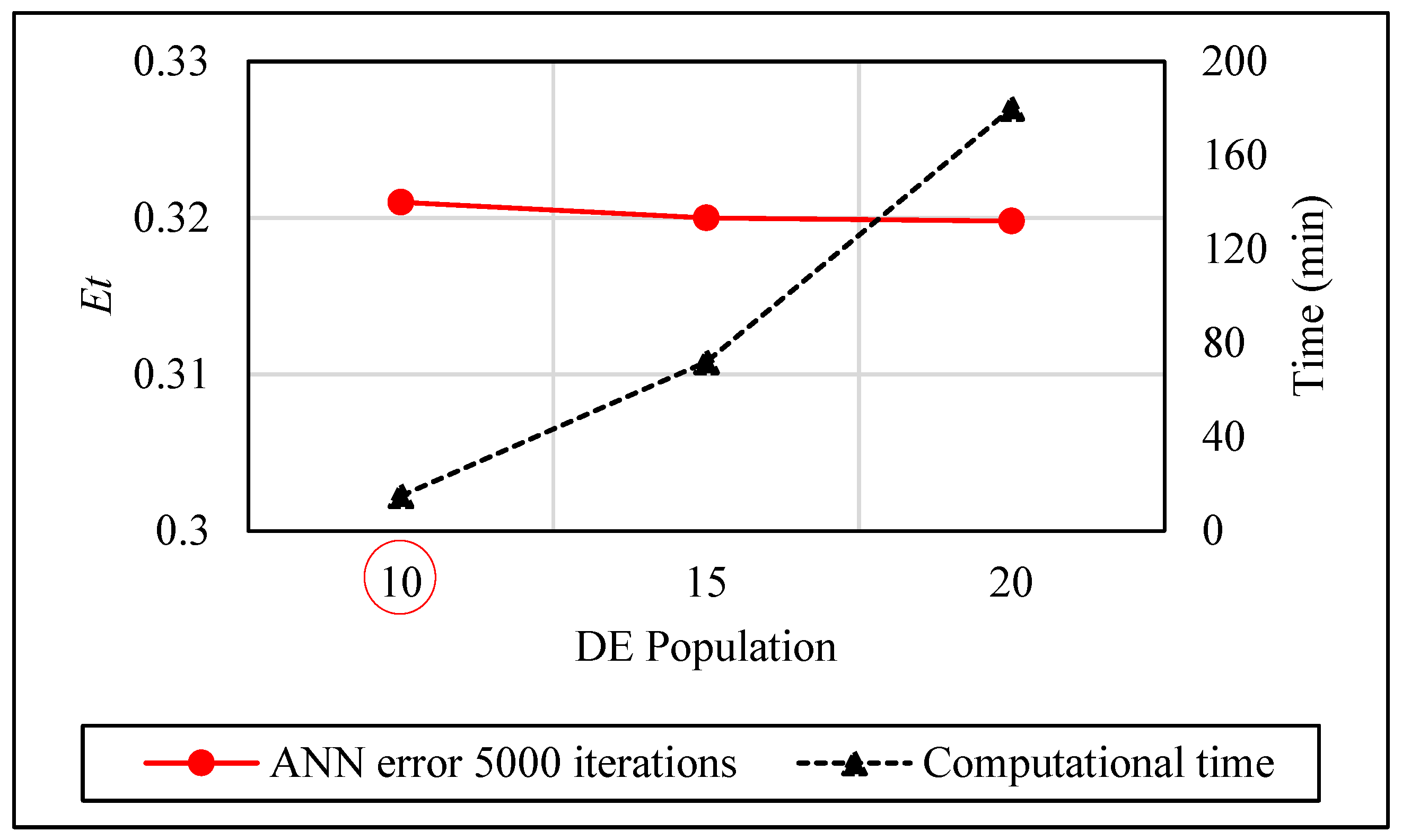
Initial optimizations were performed by setting the population size of the DE to 10, 15 and 20, and the number of iterations was equal to 5000.
Figure 9 presents the results with
Et and the computational time spent on each condition.
The variation observed in , ranging from the minimum to the maximum, is marginal at 0.002 (0.6%). In contrast, the disparity between the optimal time (15 min) and the maximum time (180 min) is substantial, amounting to 165 min (1100%). Consequently, a population size of 10 is selected for subsequent tests, considering the discernible impact of time duration on the performance metrics.
5.3. ANN Optimization
With the DE population set to 10, it is possible to analyze the effect of varying the number of optimization iterations on the performance of the overall algorithm.
Figure 10 shows the evolution of the performance index
Et.
As anticipated, an increased number of iterations leads to a reduced Et. The optimal outcome, achieving an Et of 0.296, was observed after 80 min of processing, while the least favorable result, marked by an Et of 0.321, occurred within 50 iterations and 6 min. It is noteworthy that computational time holds significance solely during the validation phase, as all parameters are fixed and incur minimal computational costs in the testing phase. The training duration is relatively brief, exerting negligible influence on the subsequent test phase.
In the testing stage, the optimum result features an Et value of 0.395, corresponding to 5000 iterations of the ANN. Conversely, the least favorable outcome was encountered with 50 iterations of the ANN, yielding an Et of 0.408. The simulation conducted with 500 iterations demonstrates intermediate Et values.
A marginal disparity of 3.45% is observed in the Et outcomes across the three examined cases, implying a nuanced progression in values with the augmentation of ANN iterations. This underscores the need to carefully assess the cost–benefit ratio associated with increasing iterations, even in scenarios demanding real-time simulations. Notably, a computational time that is approximately thirteen times shorter resulted in a mere 0.01 reduction in error, emphasizing the importance of considering efficiency gains against computational expenses.
Regarding convergence, a discernible pattern emerges from the validation results, illustrating that an increased number of iterations yields improved predictive outcomes at the expense of higher computational costs. This alignment with the anticipated behavior of ANNs was foreseen in accordance with existing definitions [
20]. It is essential to acknowledge, however, that an augmented number of iterations may also precipitate overfitting, a phenomenon outlined by Leshno and Spector [
66]. Nevertheless, it is noteworthy that such overfitting tendencies were not observed in the outcomes of the test phase.
Table 8 shows the optimized ANN architecture by the DE algorithm for different numbers of iterations. As the initial generation seeds for the DE and the ANN were fixed, the optimization procedure was conducted once.
Table 8 reveals that the optimal ANN configuration consists of three layers, three neurons, a logistic activation function, and a
α value of 0.049. The utilization of 5000 iterations resulted in this configuration, underscoring that a higher rate of learning, represented by the
α parameter in updating learning weights, yielded superior outcomes for the DE technique.
Insights gleaned from the work of Ding et al. [
67] elucidate that the neural network employing the logistic activation function in our study mitigates the gradient vanishing problem, a concern typically observed in networks with no more than 5 hidden layers. This constraint aligns with the findings outlined by Rasamoelina et al. [
68].
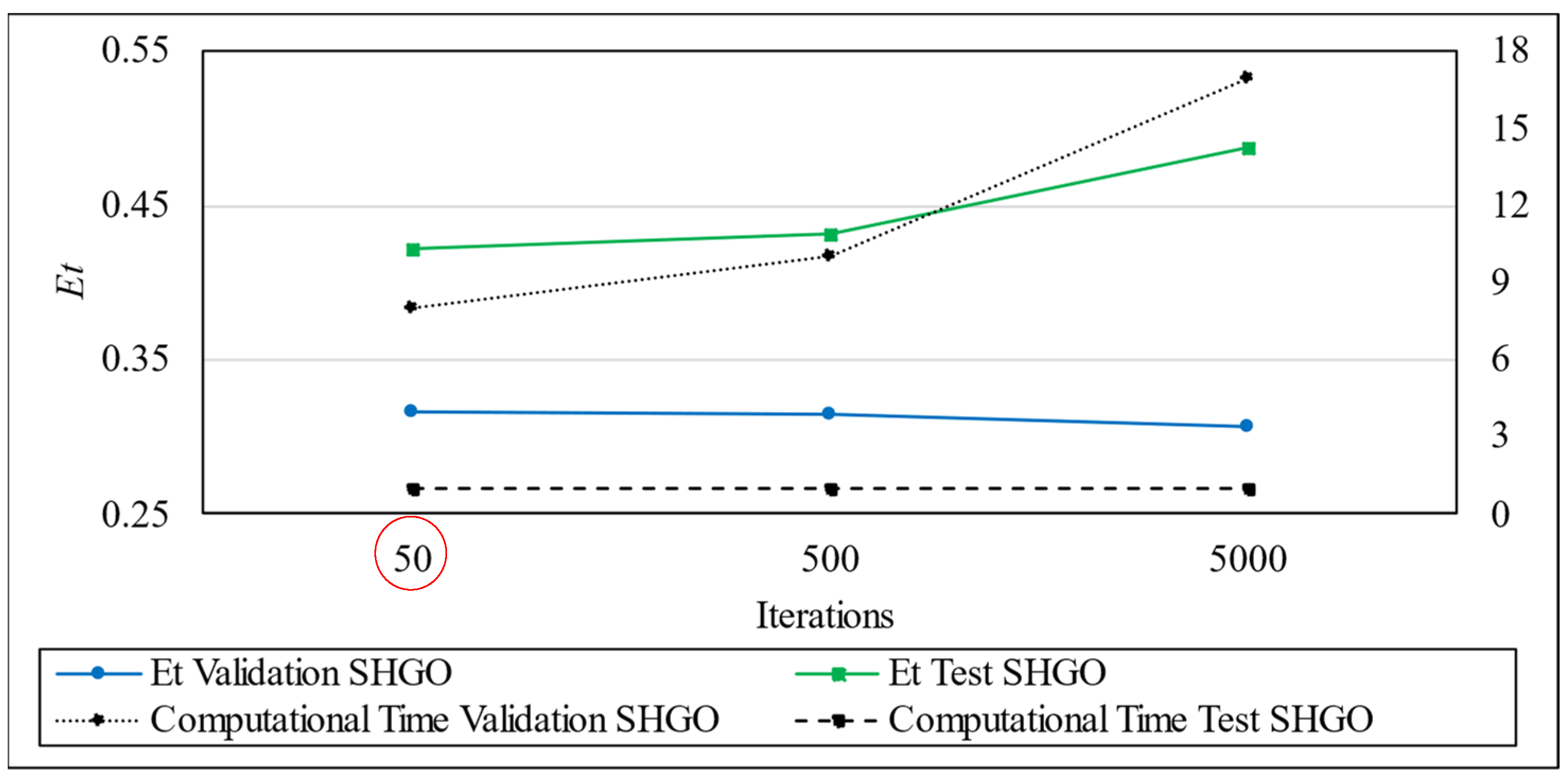
In the same scenario described before, the SHGO algorithm was also employed for optimizing the ANN architecture. The results obtained are shown in
Figure 11 and optimal architectures presented in
Table 9.
The best results from test phase are found with 50 iterations, with an Et of 0.421. Time spent varies from 8 to 17 min for 50 and 5000 iterations, respectively, in validation.
As evident, comparable ANN architectures are identified using the DE and SHGO algorithms for both 50 and 5000 iterations, differing primarily in the learning rate values. Notably, at 500 iterations, distinct optimal architectures emerge. Subsequently, a comprehensive comparison between these ANN configurations is undertaken.
Emphasis should be placed on the optimization process, which relies on minimizing the error term (Et) calculated on the validation dataset. During the subsequent test phase, the ANN is subjected to five novel inputs, allowing an assessment of its generalization capacity while verifying the absence of overfitting.
5.4. Comparison Between DE and SHGO
Figure 12 presents the performance of the ANNs determined with DE and SHGO techniques for test and validation datasets as the number of iterations increases.
Evidently, there is a discernible improvement in the error term (Et) as the number of iterations increases, with DE consistently demonstrating superior performance in both validation and test phases. Consequently, DE was chosen as the optimization technique for the subsequent sections of this paper. The focus will shift to comparing various strategies aimed at mitigating the challenges posed by the limited dataset, starting with the implementation of LOO cross-validation.
5.5. LOO Cross Validation
For a better understanding of the results of the LOO,
Figure 13 is presented, which shows the average of the errors found and the time spent on the technique in validation.
In the validation phase, the error term (
Et) exhibits a notable reduction, ranging from 0.221 at 50 iterations to 0.181 at 5000 iterations, signifying an 18.1% decrease. Correspondingly, the time required for the optimization process demonstrates an inverse relationship, escalating from 3 to 52 min, representing a substantial 1733% increase. This observation underscores the trade-off between computational time and error minimization.
Figure 14 provides a visual representation of a similar analysis conducted for the test phase.
The optimal average error term (
Et) of 0.176 is achieved with 5000 iterations, contrasting with the least favorable outcome observed at 50 iterations, yielding an
Et of 0.286. Notably, these values are approximately half of those obtained without the implementation of the LOO cross-validation technique in the test phase. This underscores the utility of LOO in addressing challenges associated with limited samples in a MAG welding dataset. While Wong [
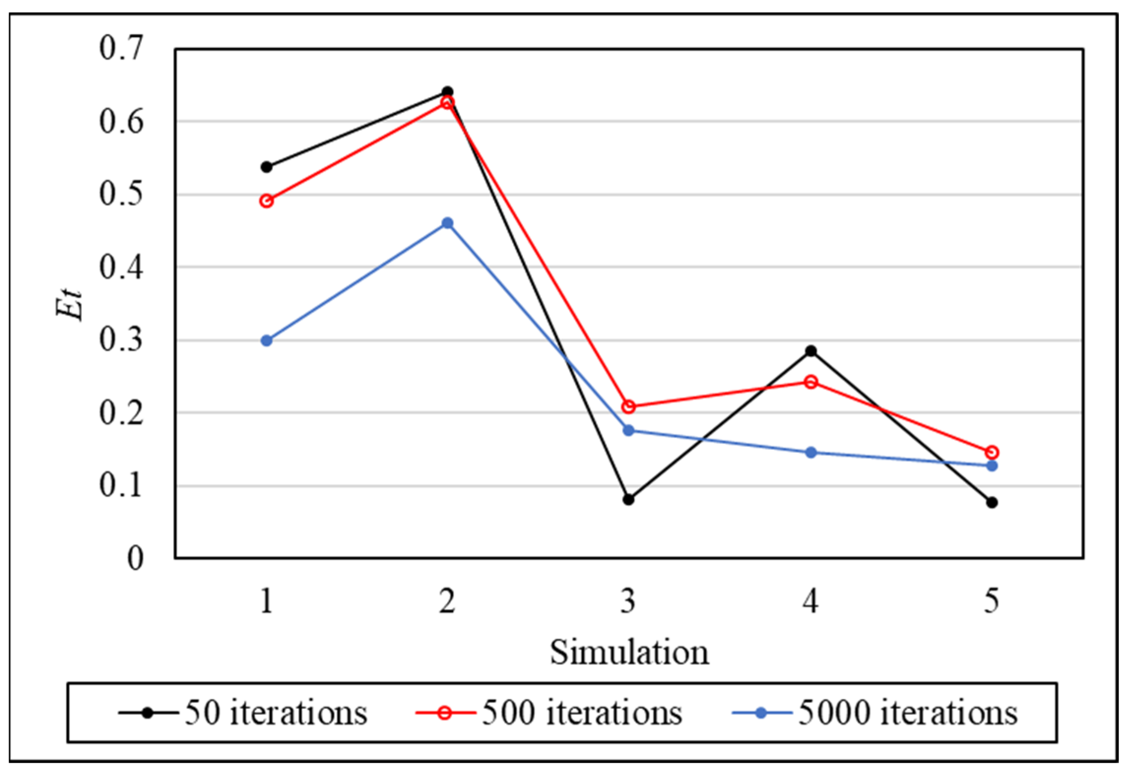
61] also, highlights improvements with the LOO cross-validation algorithm, it is crucial to note that the referenced work does not specifically pertain to welding issues.
Figure 15 further elucidates the point-by-point analysis of LOO under the three tested conditions.
Consistent with the trends observed in the average values, a higher number of iterations generally correlates with improved outcomes, except for points 3 and 5 at 50 iterations. This aligns with the findings of Nah et al. [
69], emphasizing that an increased number of iterations does not universally ensure superior results. For a more granular understanding of each result,
Table 10 provides the optimized ANN architecture parameters with 50, 500, and 5000 iterations, facilitated by the implementation of DE with LOO cross-validation.
The results indicate more pronounced convergence in terms of activation function, layers, and neurons with 5000 iterations, highlighting the enhanced convergence capability of the ANN with this iteration count. Notably, only two points experienced a change in activation function from logistic to the identity function with 50 iterations, suggesting that, in most instances, convergence for activation function within these architecture parameters had been attained with 500 iterations.
The identity activation function is exclusively observed in the context of 50 iterations. Given its simplicity and lower computational cost, it is more prevalent in simulations with fewer iterations. However, despite its simplicity, it does not equate to subpar results. This is exemplified by Wanto et al. [
70], where a linear activation function achieved a remarkable accuracy of 94%, the highest among those tested, in a population density prediction ANN.
The parameter α exhibits the most substantial variation as it increases with iterations, suggesting that each dataset necessitates a distinct optimal learning rate to achieve the best results for the studied case.
Determining the best values of
α is not a trivial task, as it depends on the dataset, the network architecture and the specific problem being addressed. Currently, it has been using techniques of adaptive control of the learning rate, as proposed by the DE in the present work. Most works use an adaptive learning rate that decays during training, however some proposals such as the present in Takase et al. [
71], which uses a rate that can increase or decrease based on the ANN prediction results.
With the evaluation of cross-validation being considered a practice with good results, it is necessary to understand the effect of data augmentation techniques, which will be addressed in the next items.
5.6. Data Augmentation
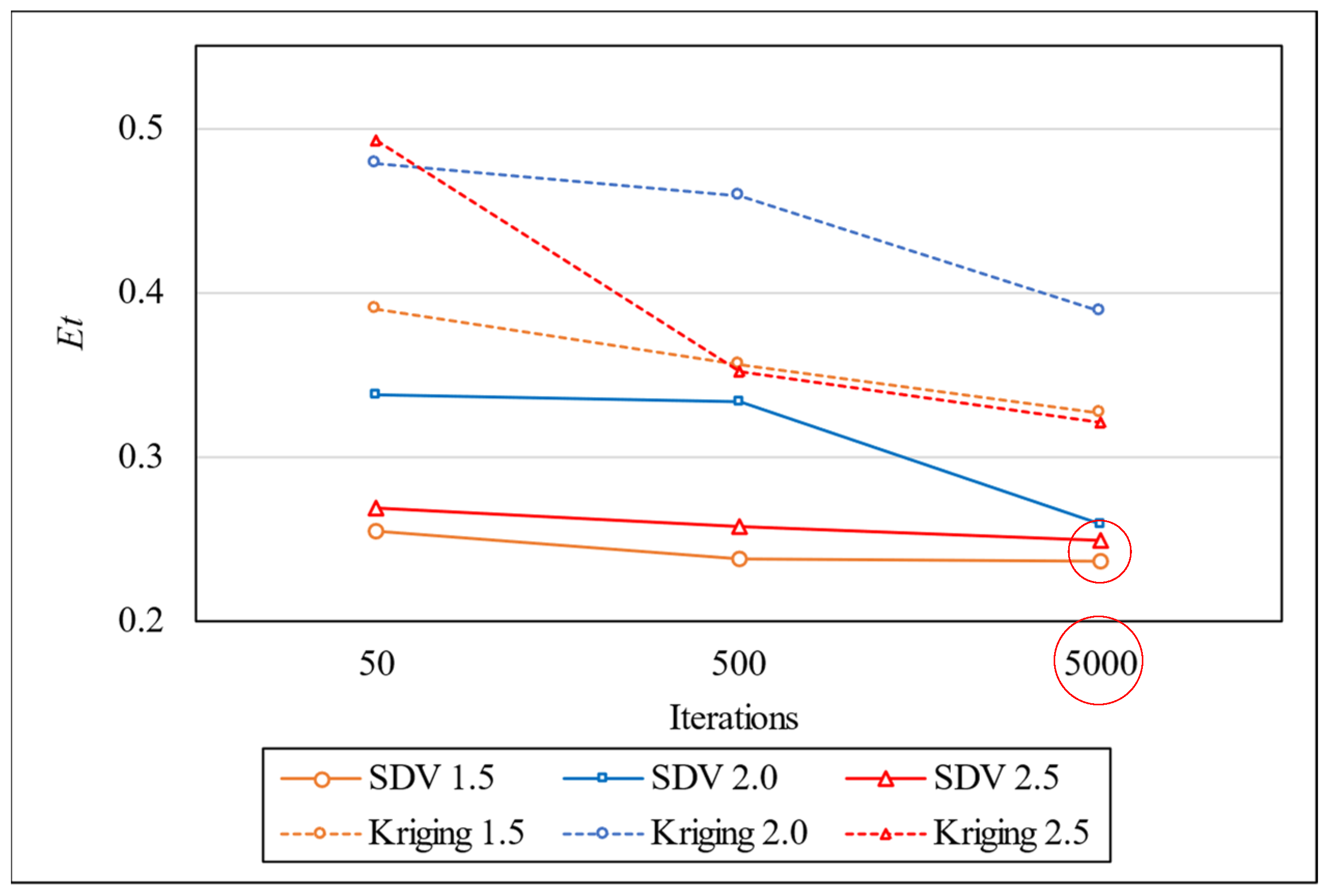
The performance indexes for the adopted data augmentation techniques (Kriging and SDV) are presented in
Figure 16 for different numbers of optimization iterations. As aforementioned, such techniques were employed to increase the dataset by 150%, 200% and 250%.
Table 11 contains the optimal architecture for each scenario. It can be noted that the DE was able to find better architectures from the dataset augmented with SDV. The smallest validation error was obtained by augmenting the training set on 1.5× by employing SDV and performing 5000 iterations of DE.
In the optimal condition for Kriging (1.5), the best result is 0.408, achieved with 5000 iterations, while the least favorable outcome is 0.804 with 500 iterations in the 2.5 condition. Regarding data generation techniques, the most favorable results are attained using the Synthetic Data Variance (SDV) technique, surpassing even the outcomes from the dataset without synthetic data. This improvement aligns with findings in Moreno-Barea et al. [
72], where the generation of additional data in a limited dataset demonstrated enhanced accuracy in predictions.
To comprehensively assess SDV and Kriging alongside standard results from the original dataset and Differential Evolution (DE), an evaluation is proposed under three conditions of sample increase: 50% (1.5), 100% (2), and 150% (2.5) for both data augmentation techniques. This comparative analysis is illustrated in
Figure 17.
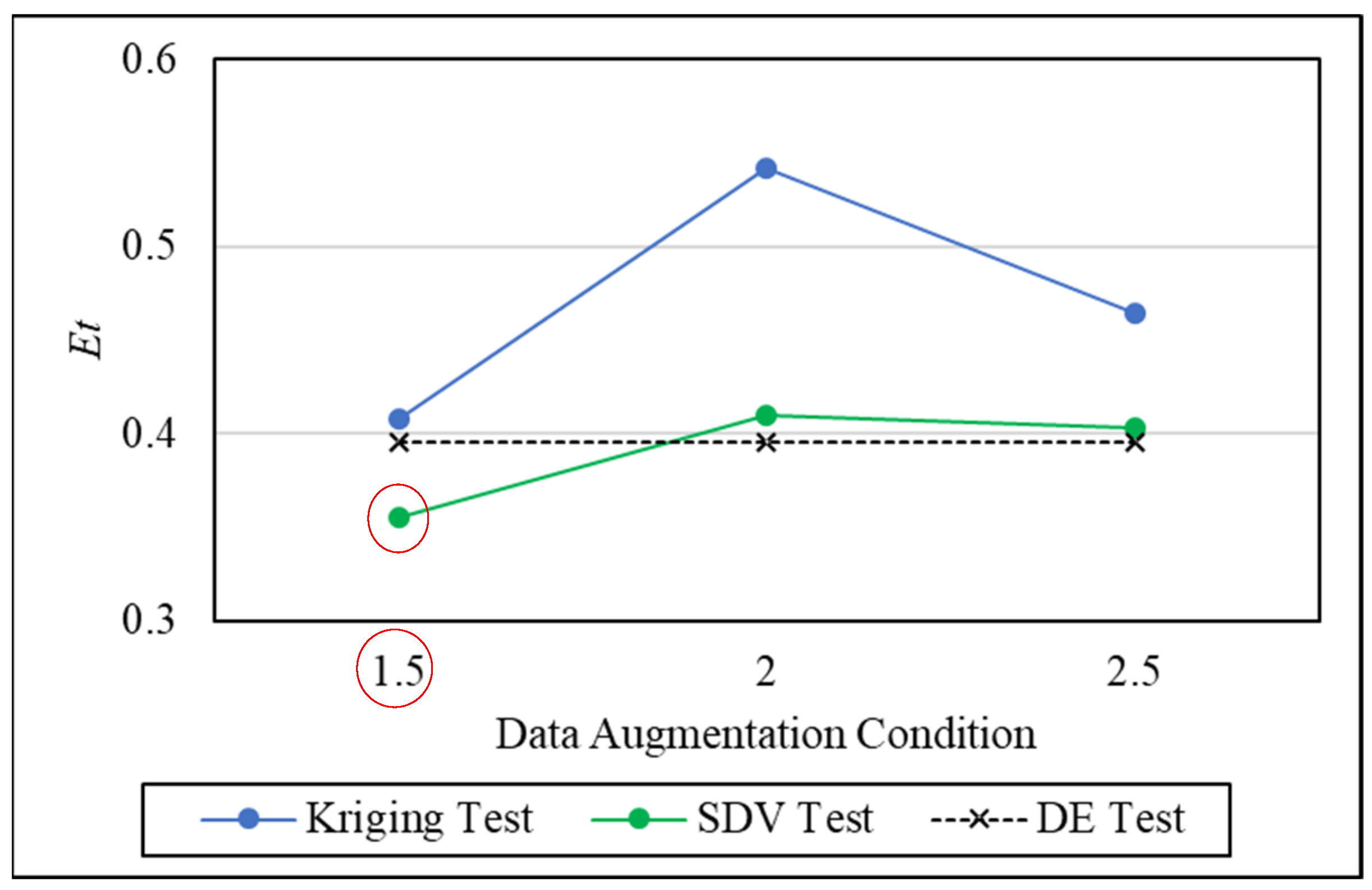
Figure 18 shows the performance index
Et on test set.
Initially, it is crucial to note that the results presented reflect the optimal iteration conditions achieved for each technique. In other words, the outcomes showcase the best results obtained for each dataset augmentation condition and technique. As depicted in
Figure 18, augmenting the dataset by 1.5× with the SDV technique led to improved values of the error term (
Et) compared to the standard DE test condition. This underscores the practicality and effectiveness of augmenting sample sizes.
To be specific, the most favorable result for SDV was achieved with a 50% increase in data, augmenting the dataset from 44 to 66 samples. This resulted in a notable reduction in the test Et value from 0.394 in the original condition to 0.355, signifying a 10.98% improvement.
Contrastingly, in the case of Kriging, no condition of data augmentation outperformed the original dataset. This suggests the impracticality of employing the Kriging technique for the welding data under consideration.
5.7. KNN and RVM
Figure 19 and
Table 12 present the results of the KNN and SVM models applied to the same nine test points used in the standard ANN condition. The performance of these models is evaluated based on the mean absolute percentage error (MAPE) across all predicted outputs, providing a clear comparison with the ANN baseline.
The analysis of the individual prediction errors for each test sample, as presented in
Figure 19 and
Table 12, provides valuable insights into the performance of the KNN model. For most test points, KNN consistently demonstrates lower prediction errors compared to the baseline, with notable improvements in several cases. Specifically, the largest error reduction was observed for Test Sample 2, where the error decreased from 0.429 to 0.316, representing a relative improvement of approximately 26%.
Conversely, there are cases where the KNN model did not yield improvements, as seen in Test Sample 3, where the error increased from 0.155 to 0.252, indicating a potential limitation of the model in certain scenarios. However, on average, the KNN model achieved a lower error (0.175) compared to the baseline (0.187), demonstrating a modest but consistent improvement of approximately 6.4% across the test set.
These results reinforce the value of incorporating alternative models such as KNN for benchmarking purposes in small datasets, while also highlighting the importance of understanding the specific behavior of each model on individual data points.
5.8. Benchmarking of Techniques
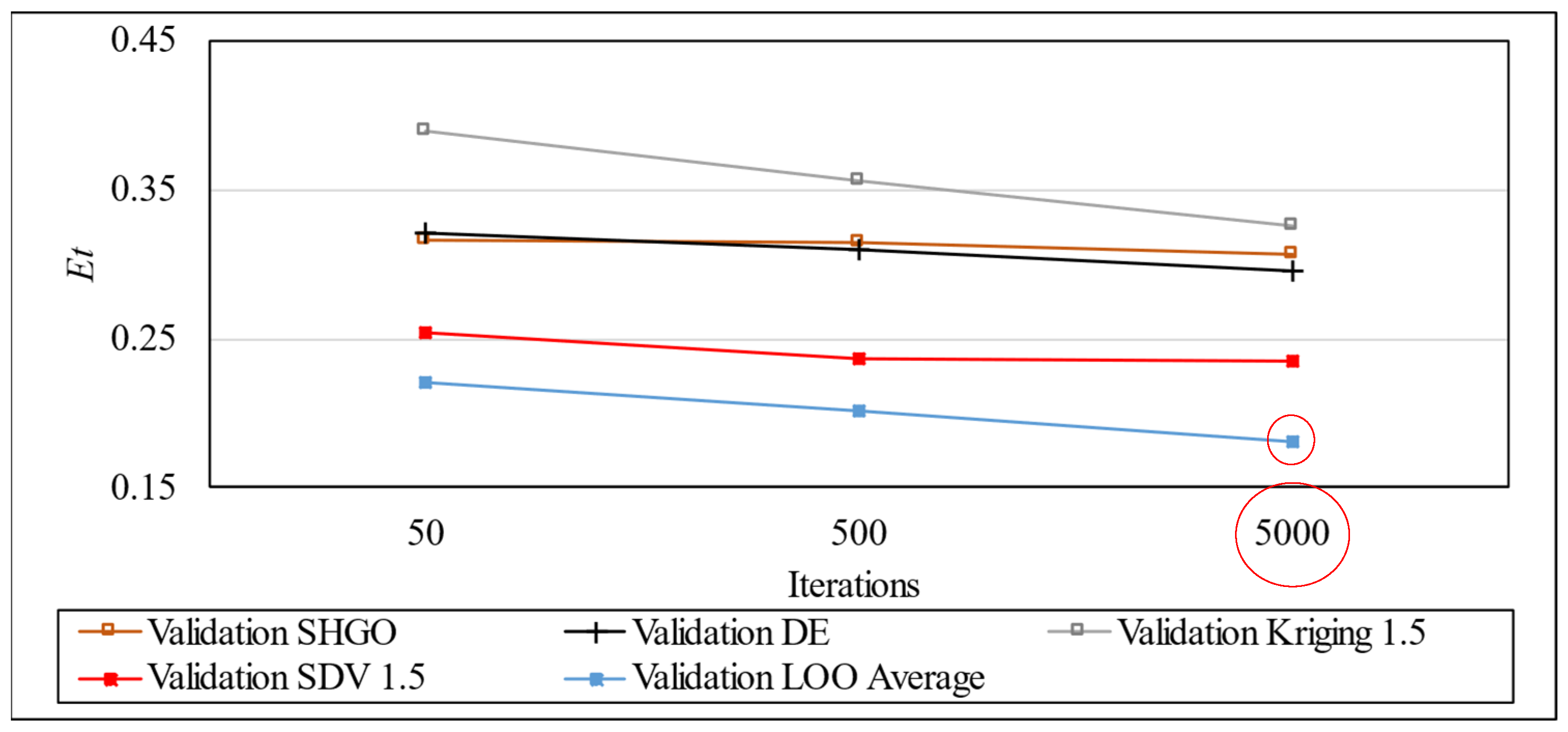
Now, all the techniques with its best results of
Et from validation phase are analyzed in the same graph in
Figure 20. KNN and SVM techniques do not use the validation phase and it is not shown on the validation section.
From validation point of view, the ranking of performance of Et stands out as follows:
Cross Validation: LOO.
Synthetic Data Vault: SDV.
DE Optimization with the original dataset.
SHGO with the original dataset.
Data Augmentation by Kriging.
It is important to highlight that validation is a previous phase in the simulation where the results can be affected by overfitting because the optimization algorithm is reaching the lowest error of the set of data used in this stage and for this reason, the test phase is performed with other sets of data to avoid overfitting and is the best result to be considered. The best results comparison of test phase is shown in
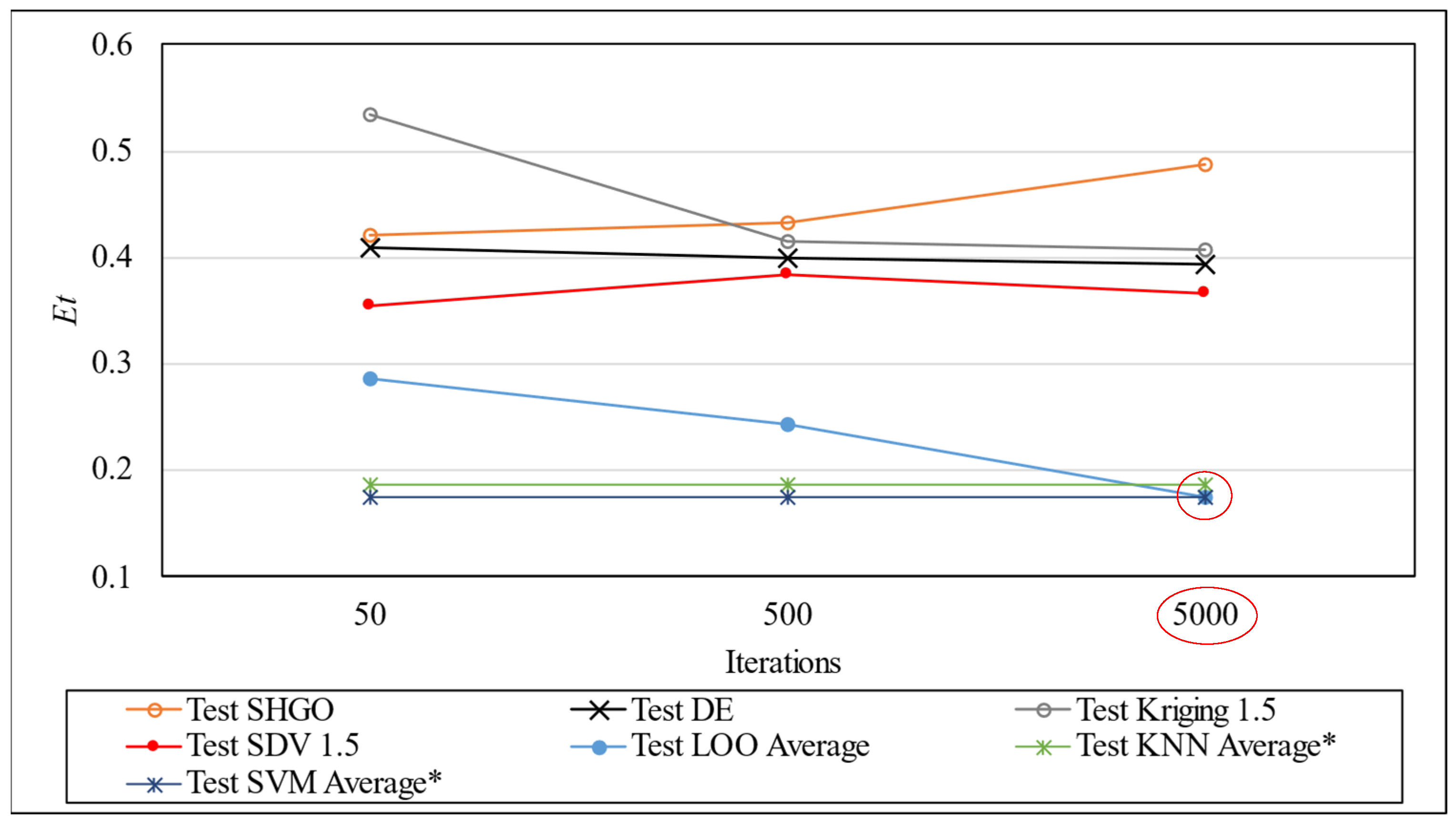
Figure 21. Finally,
Figure 22 shows the comparison between the training/validation and test phase.
The results of the KNN and SVM techniques do not use the variation in the number of iterations and are presented in the graph in
Figure 21 with constant values for each iteration value for comparative purposes only.
The test ranking in terms of error performance (Et) is shown below:
Support Vector Machines (SVM).
Cross Validation: LOO.
K-nearest Neighbors (KNN).
Synthetic Data Vault: SDV.
DE Optimization with the original dataset.
Data Augmentation by Kriging.
SHGO with the original dataset.
Each of the techniques was compared with others for the same purpose to define the best feasibility for the case of MAG welding in question. SVM machine learning technique stands out as the best alternative to the problem generated by small datasets as seen in the work of Li et al., 2021 [
47]. Cross-validation also presents competitive results compared to machine learning techniques, with a small difference from the best result. KNN also presents a result close to the two previously mentioned, proving its performance as in the study developed by Mishra et al., 2022 [
45]. The SDV technique is an alternative to the problem, with improved ANN results from the original condition. It also proves the validity of each ANN techniques used, with greater or lesser associated errors, managing to find optimal values of architecture parameters without the use of trial-and-error methods as reported by Moghadan & Kolahan [
17] for a complex problem with multiple inputs and outputs in a reduced welding dataset.
5.9. Weld Application
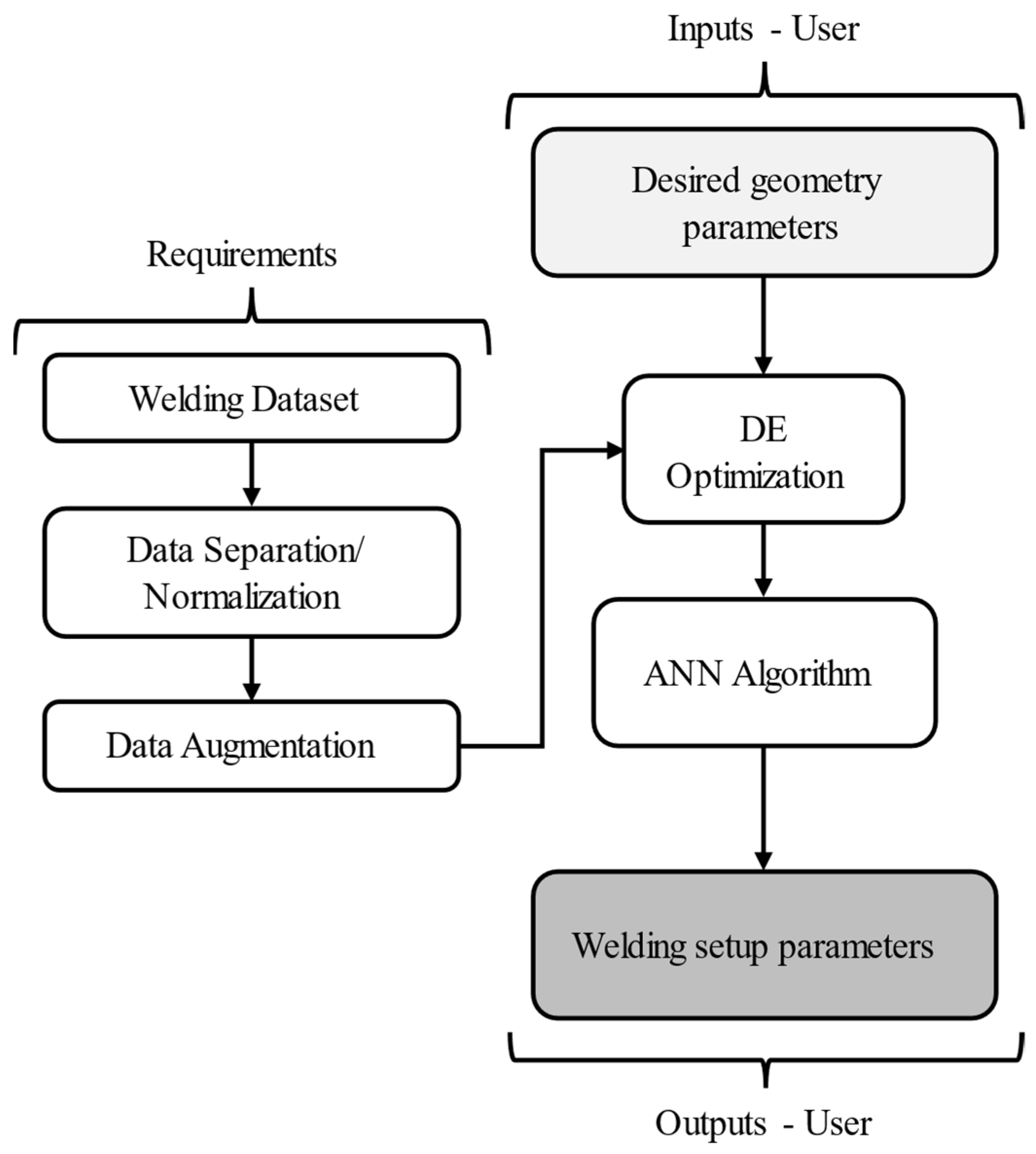
Based on all techniques implemented,
Figure 23 illustrates the overall scheme developed for data processing and prediction flow application in this work. The process starts with the input of the desired weld bead geometry parameters, including plate thickness, bevel type, gap, bead height, and width, which represent the target characteristics of the weld to be achieved. These inputs are passed to the trained prediction model—comprising the optimized ANN and comparative machine learning models (KNN and SVM)—which act as an inverse modeling system. The model processes the input geometry to estimate the appropriate welding setup parameters: voltage, gas flow rate, wire feed speed, and stickout. These predicted process parameters can then be directly applied in the welding configuration to reproduce the desired bead characteristics.
6. Conclusions
This study undertook the development and comparison of multiple techniques aimed at enhancing prediction performance using an ANN with backpropagation. The proposed algorithm empowers welders to specify desired weld bead characteristics, and the program generates the most suitable welding parameters, thereby eliminating the need for preliminary trials. This advancement streamlines the welding process, minimizes material waste, and ensures a more consistent weld quality, directly addressing common challenges faced in industrial welding operations. Additionally, the use of randomly generated experimental data reflects the variability observed in real-world welding scenarios, making the algorithm more robust and applicable across diverse practical conditions. These techniques were designed to incorporate welding parameters derived from geometric variables in MAG welding and the conclusions are presented as follows:
To avoid overfitting, it is necessary to define the architecture parameters for ANN before the test. This means using a validation and test stage with different sets of data.
The original dataset was subjected to optimization using the DE and SHGO algorithms to identify optimal ANN architecture parameters showing viability of both techniques. The results favored 5000 ANN iterations in validation stage, but in test phase the results are not convergent to an iteration number because all ANN parameters were defined just for the data of validation.
DE algorithm demonstrated superior effectiveness, but slower convergence compared to the SHGO algorithm. Iteration analysis revealed improved prediction error for output variables, with values of 0.394 for DE and 0.408 for SHGO, showing a very small difference in the techniques.
Analysis of activation functions highlighted the prominence of logistic function in achieving optimal results. As iterations progressed, the linear function’s effectiveness diminished, underscoring the need for complexity in enhancing outcomes.
The number of layers and neurons in the best results are greater than or equal to 2. These parameters played a pivotal role in enhancing predictive performance.
Among the optimization outcomes, parameter α exhibited notable variation, reflecting its sensitivity to precise calibration in each technique.
Comparative analysis addressed the impact of Synthetic data generation (SDV) and Kriging techniques on prediction outcomes. A 50% dataset increase was examined, resulting in improved prediction errors of 0.355 for SDV and 0.408 for Kriging.
Notably, SDV outperformed Kriging in all conditions of data augmentation. Further investigation revealed that 50% more synthetic data is the limit to outperform the original dataset.
The leave-one-out (LOO) technique emerged as exceptionally effective in cross-validation scenarios. Results surpassed those obtained from alternative techniques in the welding dataset, with the best error rate recorded at 0.176, markedly lower than other methods.
The result extracted from SDV 1.5 test condition (the best result excluding the LOO technique) presents 1 layer, 2 neurons, α of 0.0632 and logistic activation function.
The best result from SDV presented 10.1% and the LOO 55.3% of improvement compared to the standard best DE condition achieved.
The KNN model (0.187) demonstrated a 52.5% improvement over the baseline DE condition, while SVM achieved the best overall performance (0.175) with a 55.6% improvement.
By systematically evaluating various techniques, optimizing ANN architectures, avoiding overfitting, and investigating the influence of key parameters, this study has contributed valuable insights for enhancing prediction accuracy in welding parameter forecasting. The identified trends and recommendations open avenues for advancing the field of manufacturing processes and predictive modeling.
This study enhances the scientific understanding of using ANNs for welding by incorporating parameter optimization through DE and leveraging data augmentation methods to overcome data scarcity challenges. These advancements reduce trial-and-error efforts, improve operational efficiency, and promote consistent weld quality, effectively tackling key issues encountered in industrial welding practices. Furthermore, the integration of diverse and randomized experimental data ensures practical relevance, bridging theoretical developments with real-world applications in welding processes.
As part of the benchmarking analysis, KNN and SVM models were also implemented to evaluate alternative machine learning techniques for small datasets. These results confirm the suitability of SVM in small-sample scenarios and highlight the importance of comparing different approaches when developing predictive models for welding applications.
This study is limited to a specific welding process and dataset size. Future research should explore generalization across different materials and welding techniques, with larger and more diverse datasets. Additionally, expanding the ANN framework into real-time industrial applications with user interfaces can bridge the gap between academic models and field deployment. Another limitation of this study lies in the relatively small original dataset (44 samples), which can affect the generalizability of the proposed model. While data augmentation was employed to partially address this issue, further validation with larger and more diverse datasets is recommended. To gain a broader understanding, it would be beneficial in future works to test it on other manufacturing processes as well. Each dataset requires a tailored parametric optimization of the neural network to achieve optimal performance, meaning the same parameters cannot be applied universally.


