Article

PLSCO: An Optimization-Driven Approach for Enhancing Predictive Maintenance Accuracy in Intelligent Manufacturing

by
Aymen Ramadan Mohamed Alahwel Besha
,
Opeoluwa Seun Ojekemi
,
Tolga Oz
and
Oluwatayomi Adegboye
*
Business Administration Department, Institute of Graduate Research and Studies, University of Mediterranean Karpasia, Mersin 10, Northern Cyprus, Lefkosa 99010, Turkey
*
Author to whom correspondence should be addressed.
Processes 2025, 13(9), 2707; https://doi.org/10.3390/pr13092707 (registering DOI)
Submission received: 30 July 2025 / Revised: 16 August 2025 / Accepted: 20 August 2025 / Published: 25 August 2025

Abstract

Predictive maintenance (PdM) is a cornerstone of smart manufacturing, enabling the early detection of equipment degradation and reducing unplanned downtimes. This study proposes an advanced machine learning framework that integrates the Extreme Learning Machine (ELM) with a novel hybrid metaheuristic optimization algorithm, the Polar Lights Salp Cooperative Optimizer (PLSCO), to enhance predictive modeling in manufacturing processes. PLSCO combines the strengths of the Polar Light Optimizer (PLO), Competitive Swarm Optimization (CSO), and Salp Swarm Algorithm (SSA), utilizing a cooperative strategy that adaptively balances exploration and exploitation. In this mechanism, particles engage in a competitive division process, where winners intensify search via PLO and losers diversify using SSA, effectively avoiding local optima and premature convergence. The performance of PLSCO was validated on CEC2015 and CEC2020 benchmark functions, demonstrating superior convergence behavior and global search capabilities. When applied to a real-world predictive maintenance dataset, the ELM-PLSCO model achieved a high prediction accuracy of 95.4%, outperforming baseline and other optimization-assisted models. Feature importance analysis revealed that torque and tool wear are dominant indicators of machine failure, offering interpretable insights for condition monitoring. The proposed approach presents a robust, interpretable, and computationally efficient solution for predictive maintenance in intelligent manufacturing environments.

1. Introduction

The significance of maintenance has increased throughout the years with extensive mechanization and automation. Maintenance now plays a crucial role in the industrial sector, and its expenses account for a substantial portion of the manufacturing costs of an enterprise [1]. Existing literature broadly outlines three primary maintenance methods; namely, Corrective Maintenance (CM), Preventive Maintenance (PM), and PdM methods [2]. CM is the simplest and consists of fixing the equipment only after failure. While simple, CM often results in expensive production interruptions and unscheduled component replacements. PM involves scheduling regular maintenance tasks for specified equipment to reduce the probability of failures. Maintenance is performed while the machine remains operational to prevent unforeseen malfunctions and the resultant downtime and expenses [3,4]. While PM may decrease repair expenses and unanticipated downtime, it leads to superfluous maintenance. The assessment of when equipment will wear out relies on an assumed failure rate rather than empirical data regarding the state of the particular equipment. This frequently leads to expensive and entirely superfluous maintenance activities, resulting in increased planned downtime and necessitating complex inventory management [5]. Figure 1 illustrates the hierarchy of maintenance strategies.
Introduced as a more advanced approach, PdM or condition-based maintenance is designed to anticipate equipment failures and determine the appropriate maintenance actions to optimize the balance between maintenance recurrence and the associated expenses. PdM relies on the predictive analysis of data gathered from sensors and meters linked to equipment, historical maintenance records, and operational logs to determine when equipment requires maintenance or withdrawal. PdM enables firms to enhance their operations by performing maintenance activities only when absolutely necessary [7]. As the complexity of industrial systems grows and the amount of data generated increases, Machine Learning (ML) has been increasingly applied to predictive maintenance and has notably enhanced its effectiveness. ML algorithms have demonstrated the ability to manage high-dimensional and multivariate data, uncover hidden links within data in intricate and dynamic contexts, and deliver unparalleled accuracy in failure prediction [8,9]. Common ML algorithms include Support Vector Machines (SVM) [10], K-Nearest Neighbors (KNN) [11], Recurrent Neural Networks (RNNs) [12], Decision Trees (DT) [13], Bayesian Networks (BN) [14], Long Short-Term Memory networks (LSTMs) [15], Convolutional Neural Networks (CNNs) [16], Gradient Boosting Machines (GBM) [17], Random Forests (RF) [18], Naive Bayes (NB) [19], K-means clustering [20], and the Extreme Learning Machine (ELM) [21]. ELM stands out among other ML algorithms due to its rapid training process and versatility. Unlike traditional neural networks, ELM eliminates the iterative learning process, achieving faster convergence and reducing computational complexity [22]. Few studies have explored the application of ELM for predictive maintenance across various domains, including electrical systems [23], power transformers [24], aero-engines [25], lithium-ion batteries [26], and steam turbines [27].
However, ELM’s effectiveness depends heavily on parameter tuning. Manual parameter tuning is both time-intensive and frequently ineffective in attaining high-precision outcomes. To address this challenge, Metaheuristic Algorithms (MAs) are used to autonomously tune parameters via extensive simulation tests, guaranteeing that the model parameters reach ideal settings [28]. Moreover, the integration of MAs notably improves the model’s stability and generalization capacity. Van Thieu et al. introduced a combination of ELM with the weighted mean of vectors (INFO) algorithm, Pareto-like Sequential Sampling (PSS), and the Runge–Kutta optimizer (RUN) [29]. Their comparison analysis, utilizing streamflow data, demonstrates improved forecast accuracy, strong convergence, and consistent stability, especially the PSS-ELM. Li et al. developed an optimal forecasting model for supercapacitor capacity, which combines an ELM with the Heuristic Kalman Filter (HKF) technique [30]. The experiments revealed that HKF-ELM requires fewer setting parameters, reduced time cost, and higher prediction accuracy. Similarly, Boriratrit et al. proposed three hybrid forecasting models by integrating ELM with Jellyfish Search (JS-ELM), Flower Pollination (FP-ELM), and Harris Hawk (HH-ELM) algorithms to improve precision and reduce overfitting [31]. JS-ELM surpassed the other models by attaining the lowest Root Mean Square Error (RMSE) and ensuring efficient processing times. Sun and Huang presented the Whale Optimization Algorithm-ELM (WOA-ELM) for forecasting carbon emission intensity [32]. The WOA-ELM exhibited a strong ability to handle extensive datasets while proficiently accommodating smaller samples. The incorporation of the WOA significantly augmented the ELM’s performance by enhancing its accuracy and overall predictive efficacy. Tan introduced an alternative variant of ELM, a hybrid method that uses the Improved Multi-Objective Particle Swarm Optimization (IMOPSO) algorithm to optimize multiple competing objectives [33]. This technique limits the ELM network’s input weights and hidden biases to appropriate ranges, improving generalization performance and resolving instability. Hua et al. proposed a hybrid framework joining Partial Least Squares (PLS), Variational Mode Decomposition (VMD), Improved Atom Search Optimization (IASO), and ELM [34]. VMD decomposes wind speed data into frequency-based sub-series, PLS refines the dataset, and IASO, enhanced with simulated annealing, optimizes the ELM. The model outperformed other models, demonstrating superior accuracy and reliability. Kardani et al. [35] also proposed the integration of MAs, Firefly Algorithm (FFA), and Improved Firefly Algorithm (IFFA) with ELM, Adaptive Neuro-Fuzzy Inference System (ANFIS), and Artificial Neural Networks (ANN) to optimize prediction performance. Among them, the ELM-IFFA model delivered the most accurate and reliable results [35]. Gao et al. [36] developed a hybrid prediction model in which the RF is utilized to extract parameters. The ELM is then optimized for prediction using the Improved Parallel Whale Optimization Algorithm (IPWOA). Simulation experiments demonstrated that the RF-IPWOA-ELM model achieves superior prediction accuracy [36]. Shariati et al. utilized the hybrid ELM and the Grey Wolf Optimizer (GWO) to predict the compressive strength of concrete with partial cement replacements [37]. The authors reported notable improvements in the performance of the ELM-GWO model.
Despite the advancements made in integrating MAs with ELM across various applications, the adoption of ELM in PdM domains remains limited. While ELM has demonstrated significant potential in other fields, its application in other fields shows that it faces challenges stemming from limited accuracy and generalizability. These limitations primarily arise due to the random initialization of weights and biases, which, although contributing to ELM’s computational speed, hinder its ability to achieve optimal performance. Furthermore, the absence of multiple hidden layers and robust optimization strategies exacerbates these issues, particularly in complex industrial scenarios where accurate predictions are critical. Although prior studies have demonstrated the benefits of integrating MAs with ELM to enhance its predictive capabilities, the existing literature lacks approaches that incorporate novel competitive-based learning mechanisms and dynamic adaptive strategies. Such strategies are essential to ensure an effective balance between exploitation and exploration of the problem space by the optimization algorithm, enabling the identification of optimal weights and biases and thus significantly improving ELM’s accuracy and robustness. This gap in the literature forms the core motivation and impetus for this research, which seeks to address these challenges through the development of an innovative optimization framework tailored for ELM in PdM applications.
Therefore, this study introduces the integration of the PLSCO to optimize the weights and biases of ELM for PdM prediction. The PLO was introduced by Yuan et al., and it draws inspiration from the aurora phenomenon [38]. It models the behavior of high-energy particles interacting with the Earth’s magnetic field and atmosphere. PLO presents the advantage of effectively balancing local and global search processes by using adaptive weights. However, similar to other MAs, PLO can be trapped in local optima, and its convergence can be hindered in high-dimensional spaces. The PLSCO addresses these drawbacks by introducing two mechanisms into the traditional PLO. One approach to mitigate the limitations of PLO is to incorporate a CSO strategy, where the population is dynamically split into two groups: winners and losers, based on their fitness values. This division ensures a structured division of optimization roles, enhancing both exploration and exploitation. The winner group, comprising the top-performing individuals, focuses on refining local searches. These particles are updated using the PLO mechanism, which excels in fine-tuning solutions and exploiting promising regions in the search space. This ensures that high-quality solutions are further improved through focused exploitation. The loser group, consisting of the lower-performing individuals, adopts the SSA mechanism. SSA is well-suited for exploration due to its ability to simulate salp chain dynamics, which allows for broader coverage of the solution space. Unlike existing hybrid metaheuristic algorithms for ELM tuning, which frequently operate by sequentially invoking constituent algorithms, PLSCO introduces a co-evolutionary control layer that unifies the core mechanisms of PLO, CSO, and SSA into a single adaptive search framework. The collision-based exploitation mechanism from PLO is embedded directly into the swarm update equations, enabling localized refinements to occur concurrently with global exploration. The competitive learning dynamics of CSO are adapted to act as a real-time regulator of exploration–exploitation balance, informed by SSA’s leader–follower hierarchy. This integration allows PLSCO to adapt its parameter settings dynamically as the search progresses. Consequently, PLSCO offers a more synergistic and responsive search process, improving convergence behavior. A detailed comparison of the architectural components, parameter adaptation strategies, and optimization mechanisms of the proposed ELM-PLSCO framework with other benchmark ELM-based hybrid models is presented in Table 1.
The remainder of this paper is structured as follows. Section 2 presents background information on the PLO and the proposed PLSCO. Section 3 describes the novel ELM-PLSCO model, while Section 4 presents the experiments conducted and discusses their results. Section 5 provides a conclusion and outlines potential directions for future research.

2. Methodology

2.1. Polar Light Optimizer (PLO)

The PLO draws inspiration from the aurora borealis, where charged particles (solar wind) interact with the Earth’s magnetic field, creating luminous patterns in the sky as shown in Figure 2.
The algorithm incorporates three primary mechanisms: gyration motion, aurora oval walk, and particle collision, which are designed to simulate global exploration and local exploitation in the optimization process [38]. The algorithm starts with a randomly generated population of candidate solutions. The population matrix X , is given as follows in Equation (1).
X ( N , D ) = L B + R × ( U B L B ) = X ( 1,1 ) X ( 1,2 ) X ( 1 , D ) X ( 2,1 ) X ( 2,2 ) X ( 2 , D ) X ( N , 1 ) X ( N , 2 ) X ( N , D )
where N is the number of particles. D is the dimension of the solution space. U B and L B denote the upper and lower boundaries of the search space, respectively. R denotes a random value in [ 0,1 ] . To search for optimal solutions, PLO imitates the gyration motion. The gyration motion simulates the spiraling motion of charged particles under the influence of the Earth’s magnetic field, characterized by the Lorentz force as expressed in Equation (2).
F L = q v B
where q is the particle’s charge. v is its velocity. B is the magnetic field vector. The motion is further modeled using Newton’s second law in Equation (3).
F L = m d v d t
Here, m represents the mass of the charged particle. Combining Equations (2) and (3) yields the first-order ordinary differential equation, as expressed in Equation (4).
m d v d t = q v B
Integrating Equation (4) over time t from 0 to t , and velocity v 0 to v ( t ) , yields Equation (5).
v 0 v   1 v d v = 0 t   q B m d t
Solving Equation (5) yields Equation (6).
v ( t ) = v 0 e q B t m
By accounting for atmospheric damping, the equation is rewritten as expressed in Equation (7).
m d v d t = q v B α v
where α is the damping factor. This modification transforms the equation into a nonhomogeneous first-order linear differential equation. To solve it, the method of variation of constants is applied by assuming a solution of the form v = C e λ t , where C and λ are constants to be determined. First, obtain the linear first-order ODE as given in Equation (8).
d v d t = ( q B α ) m v
Seeking a solution of the form v ( t ) = C e λ t with constant C , substitution yields Equation (9).
m λ C e λ t = ( q B α ) C e λ t
After   canceling   C e λ t 0 ,   we   have   λ = q B α m ,   giving Equation (10)
v t = C   e x p q B α m t
where C is the integration constant. The parameters q , B , and C are set to 1, while m is assigned a value of 100. The damping factor α is a random variable within the range [ 1,1.5 ] . The time-dependent behavior of the velocity v ( t ) described by Equation (10) is incorporated into the algorithm to evaluate the fitness function during the optimization process. The auroral oval walk is a mechanism in the PLO that enhances global exploration of the solution space. Auroras typically form along an elliptical region known as the auroral oval, whose size and boundaries vary with geomagnetic activity and the interplanetary magnetic field. The dynamic fluctuations of the auroral oval introduce unpredictable chaos, which is beneficial for efficient global search. To model this behavior, Levy Flight (LF) is employed due to its non-Gaussian random walk characteristics. The LF step distribution is defined in Equation (11).
L e v y ( d ) | d | 1 β , 0 < β 2
where β determines stability, and d represents the step size. The auroral oval motion is described in Equation (12).
A o = L e v y ( d ) × X avg   ( j ) X ( i , j ) + L B + r 1 × ( U B L B ) / 2
Here, A o models the dynamic expansion and contraction of the auroral oval, X avg   ( j ) is the population’s center of mass; it is expressed in Equation (13).
X a r g = 1 N × i = 1 N   X ( i )
X ( i , j ) is the current position of a particle. PLO combines gyration motion for local exploitation and the auroral oval walk for global exploration. Gyration motion simulates particles spiraling along the Earth’s magnetic field lines to perform fine local adjustments, while the auroral oval walk enables larger exploratory steps to discover valuable regions in the search space. The combined position update rule is expressed in Equation (14).
X new   ( i , j ) = X ( i , j ) + r 2 × W 1 × v ( t ) + W 2 × A o
where r 2 accounts for environmental randomness ( r 2 [ 0,1 ] ), W 1 and W 2 are adaptive weights balancing gyration motion ( v ( t ) ) and auroral oval walk A o . W 1 and W 2 are given in Equations (15) and (16).
W 1 = 2 ( 1 + e 2 ( t / T ) 4 ) 1
W 2 = e ( 2 t / T ) 3
As iterations progress, W 1 increases, emphasizing local exploitation while W 2 decreases, prioritizing global exploration early on. This dynamic balance allows the PLO to efficiently explore and exploit the solution space, achieving optimal or near-optimal solutions. Robust global exploration and local exploitation alone are insufficient for a well-rounded optimization algorithm; the ability to escape local optima is equally critical. To address this, the PLO incorporates a particle collision strategy inspired by the dynamic interactions of charged particles in the solar wind as they travel toward Earth. When entering the Earth’s atmosphere and magnetic field, high-energy particles such as electrons and protons experience frequent collisions, altering their velocity and trajectory. These collisions transfer energy, trigger excitation and ionization of other particles, and contribute to the complex, evolving shapes of auroras. In the PLO, particle collisions are modeled to induce chaotic movement, enabling particles to escape local optima. The position of a particle after a collision is calculated in Equation (17).
X n e w i , j = X i , j + sin r 3 × π × X i , j X a , j , r 4 < K   a n d   r 5 < 0.05
Here, X ( a , j ) represents a randomly selected particle. The collision probability K , which increases over time, is given in Equation (18). In Equation (17), r 3 is a uniformly distributed random variable in [0,1] that controls the phase shift of the sine function, influencing the displacement magnitude following particle collisions. r 4 is a uniformly distributed random variable in [0,1] used to determine whether a collision event occurs in relation to the collision probability K . The parameter K , increases monotonically with iteration count, thereby raising the probability of collision-induced perturbations during later search stages and enhancing local search diversity. Where r 5 is an independent random variable used to add stochastic variability in collision activation.
K = ( t / T )
As the algorithm progresses, collisions occur more frequently, enhancing the ability of particles to explore new regions of the solution space. This strategy plays a crucial role in maintaining diversity and preventing premature convergence.

2.2. Proposed PLSCO

2.2.1. Salp Swarm Algorithm (SSA)

A notable limitation of the PLO lies in its tendency to exhibit reduced exploration. PLO effectively leverages the auroral oval walk for exploration. Although the auroral oval walk introduces randomness through LF, it focuses on specific candidate solutions within a limited region, reducing the likelihood of escaping local optima. Its ability to maintain a diverse population and explore uncharted regions of the solution space is relatively constrained. This limitation becomes especially pronounced in complex and high-dimensional optimization problems, where premature convergence to local optima hinders the algorithm’s overall performance. The integration of the SSA within the PLSCO directly addresses this shortcoming by introducing a dynamic mechanism to bolster global exploration. The SSA is inspired by the collective swarming behavior of salps, marine organisms that navigate and forage in a structured formation called a salp chain. In SSA, the population of salps is divided into two roles: leaders and followers [39]. The leader, positioned at the head of the chain, determines the primary movement direction by moving closer to the food source, which represents the best solution (global optimum) found so far. The followers occupy subsequent positions in the chain and adapt their movements based on the leader’s trajectory. Leader salps position is updated as follows using Equation (19) [40].
X 1 , j t + 1 = X b e s t , j t + c 1 U B j L B j c 2 + L B j ,   i f   c 3 0.5 X b e s t , j t c 1 U B j L B j c 2 + L B j ,   i f   c 3 < 0.5
where X 1 , j t + 1 is the updated position of leader salps in the j -th dimension. X best   , j t represents the current position of the best solution in the j -th dimension. U B j and L B j are the upper and lower bounds of the search space in the j -th dimension. c 1 , c 2   a n d   c 3 represent random coefficients, where c 1 controls step size, c 2 adds randomness within bounds, and c 3 determines movement direction. The parameter c 2 is a random value in [ 0,1 ] , while c 3 is randomly drawn from [ 0,1 ] . The parameter c 3 determines the movement direction of leader salps. When c 3 ≥ 0.5, the leader moves toward the food source; when c3 < 0.5, the leader moves away, enabling exploration of alternative regions. For example, if c3 = 0.7, the leader’s position update is biased toward the best-known solution, accelerating exploitation. Conversely, if c3 = 0.4, the leader moves in the opposite direction, facilitating exploration and helping to escape potential local optima. This bidirectional adjustment mechanism ensures a balanced search process. The upper and lower bounds of the j -th dimension are represented as U B j and L B j , respectively. A critical parameter, c 1 , dynamically governs the balance between exploration and exploitation and is defined in Equation (20).
c 1 = 2 e 4 t T 2
where T is the total number of iterations and t is the current iteration. For the followers, their positions are updated based on the average of their current position and the position of the preceding salp in the chain as given in Equation (21).
X i , j t + 1 = 1 2 X i , j t + X i 1 , j t
The SSA directly addresses the exploration flaw by introducing a stochastic, hierarchical leader–follower dynamic that promotes broader and adaptive exploration. SSA’s design mitigates the deterministic and localized behavior of PLO through the exploration strategy of SSA in Equation (19). Furthermore, the adaptive step size c 1 , decreases gradually over iterations, ensuring that the algorithm focuses on exploration in the early stages and transitions seamlessly to exploitation as the search progresses.

2.2.2. Competitive Swarm Optimizer (CSO)

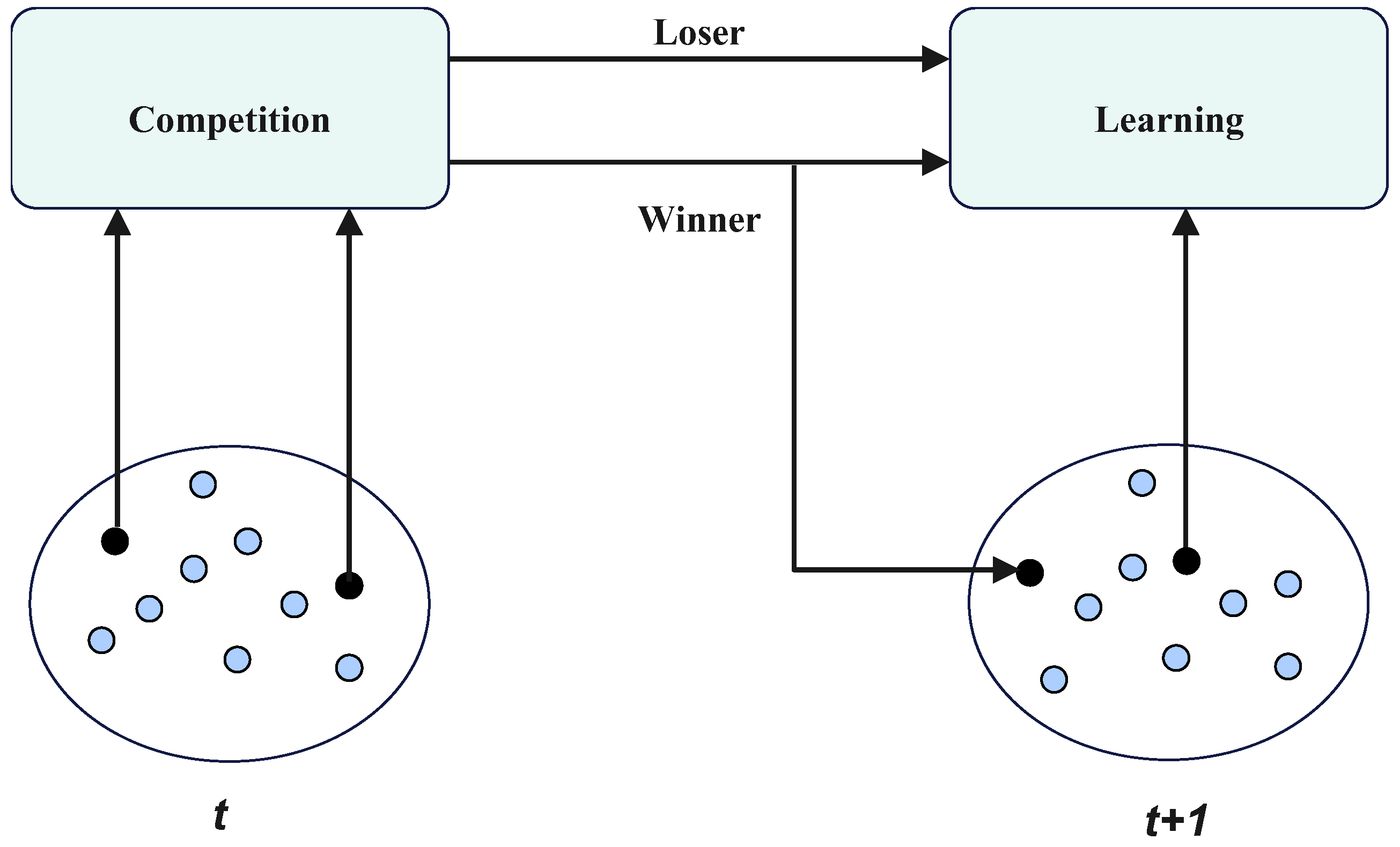
The integration of CSO into PLSCO transforms the algorithm’s exploitation phase by addressing the inherent limitations of PLO. CSO introduces a structured, adaptive approach to local refinement, ensuring that high-quality solutions are continuously improved as shown in Figure 3. This is achieved by continuously refining the best solutions and exploring regions of possible solutions with worst-performing particles. This refinement complements the global exploration capabilities introduced by SSA, creating a dynamic balance between exploration and exploitation. The CSO improves upon the PLO algorithm by introducing a competitive mechanism. The population of N search agents (set to an even number) is randomly divided into N / 2 pairs. In each pair, one agent is designated as the winner and the other as the loser, based on their fitness values. Winners are directly carried over to the next generation without modification, while losers update their velocity and position by learning from the winners. This approach ensures that N / 2 agents are updated in each iteration, preserving the optimization process of PLO while enhancing performance. The velocity and position of a loser in the c -th pair at iteration t are updated using Equations (22) and (23) [41].
V l o s e r , j t + 1 = Q 1 ( c , t ) V l o s e r , j t + Q 2 ( c , t ) X winner , j t X l o s e r , j t + ϕ Q 3 ( c , t ) X j t X l o s e r , j t
X l o s e r , j t + 1 = X l o s e r , j t + V l o s e r , j t + 1
X winner , j t is the position of the winner in the j -th dimension. X loser , j t   a n d   V loser , j t represent the position and velocity of the loser in the j -th dimension, respectively. X j t denotes the average position of the entire population in the j -th dimension. Q 1 ( c , t ) , Q 2 ( c , t ) and Q 3 ( c , t ) are random stochastic vectors in [ 0,1 ] n , influencing the learning behavior; ϕ is a predefined parameter regulating the X j t influence on velocity. For winner and loser selection, a random permutation of the population indices, denoted as r a n d l i s t , is created as the randomized pairing of agents. For each iteration of the pairing process, k represents the loop index that determines the pairs of agents being compared. r 5 represent the first agent in the pair r 5 = r a n d l i s t [ k ] , and r 6 is a second agent in the pair r 6 =   r a n d l i s t [ k + N / 2 ] . The winner and loser are determined using Equations (24) and (25) [42].
W i n n e r ( k ) = r 5 ,   i f   f i t n e s s   r 5 < f i t n e s s   r 6 r 6 ,   o t h e r w i s e  
L o s e r ( k ) = r 6 ,   i f   f i t n e s s   r 5 < f i t n e s s   r 6 r 5 ,   o t h e r w i s e  
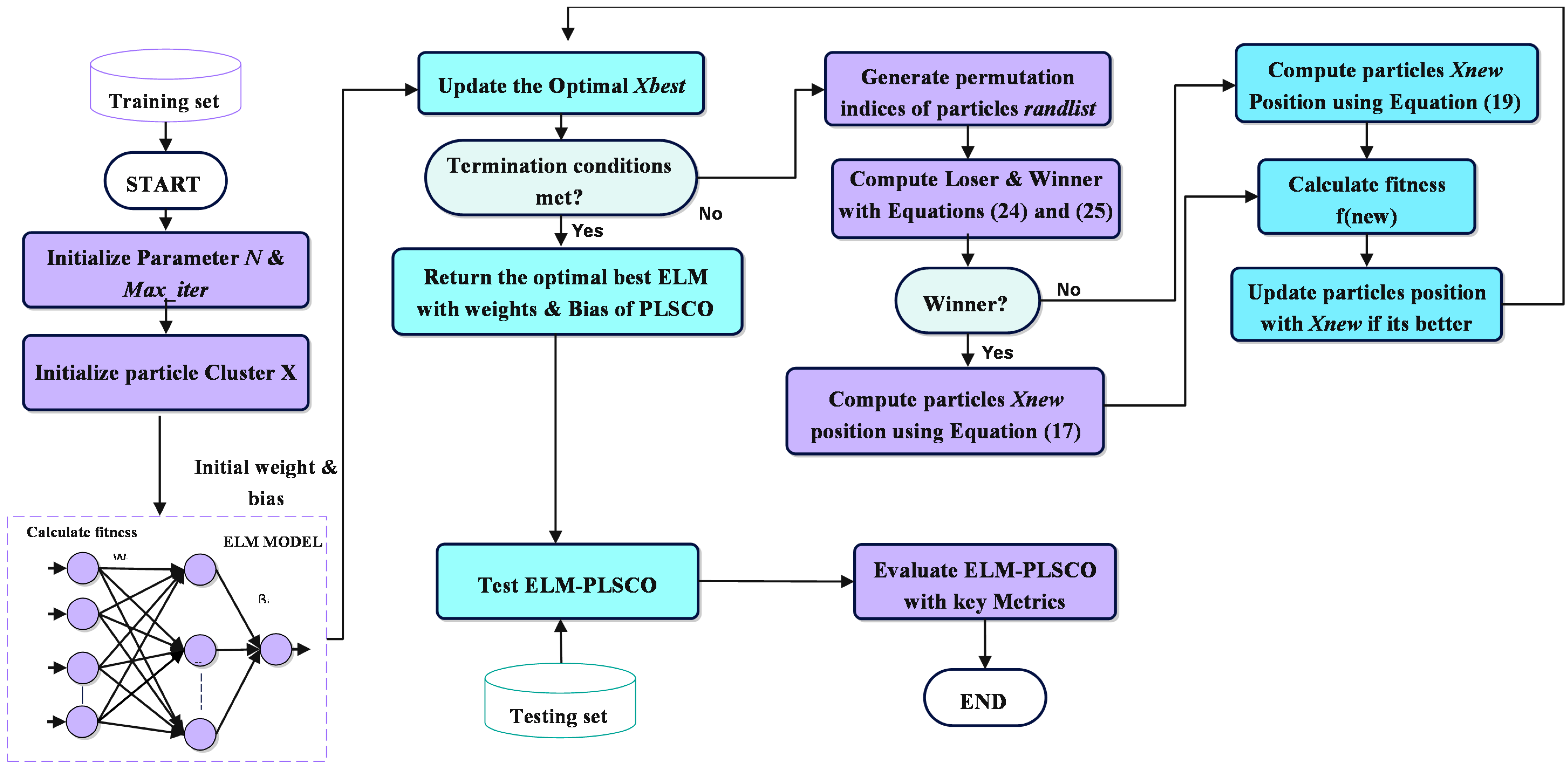
The integration of PLO, CSO, and SSA in PLSCO is a deliberate design choice based on both theoretical complementarity and empirical success reported in the recent metaheuristic literature. PLO contributes strong local exploitation capabilities through its gyration motion and auroral oval walk, supported by adaptive weighting to fine-tune solutions within promising regions. SSA introduces leader–follower dynamics that enable broad, adaptive exploration while maintaining population diversity, a feature particularly advantageous in multimodal landscapes. CSO adds a structured competition mechanism, dividing the population into winners and losers to create an adaptive feedback loop that reinforces exploitation for top-performing solutions while stimulating exploration among underperformers. The algorithm begins by initializing a population of high-energy particles, each representing a candidate solution within the search space. The fitness of these particles is evaluated based on the problem’s objective function, and the global best solution, X best ,   is identified. In each iteration, the population is randomly divided into N / 2 pairs, where N is the population size. Fitness comparisons are conducted within each pair to classify agents as winners or losers, according to Equations (24) and (25). Winners who demonstrate better fitness update their positions using the PLO mechanism as described in Equation (17). PLO emphasizes exploitation by leveraging gyration motion, auroral oval walks, and particle collisions to refine solutions in potential regions. Losers with inferior fitness update their positions using SSA as described in Equation (19), which focuses on exploration. The SSA mechanism employs leader–follower dynamics to encourage the exploration of unexplored regions, preventing stagnation in local optima and maintaining population diversity. After updating the winners and losers’ positions, each particle’s fitness is re-evaluated, and positions are selectively retained if they improve fitness. The global best solution, X best   , is continuously updated as better solutions are identified. The process iterates until the maximum number of iterations is reached or a predefined convergence criterion is satisfied, at which point the best solution, X best , is returned as seen in Algorithm 1. This competitive division incorporates an adaptive learning mechanism, where winners continue exploiting the local search space while losers enhance exploration by learning from both winners and global dynamics. By dynamically pairing agents and employing diverse update strategies, PLSCO prevents premature convergence, ensures an efficient search process, and adaptively balances global and local search efforts. This design addresses the limitations of standalone PLO and SSA, making PLSCO a robust and efficient optimization approach suitable for solving complex, high-dimensional, and multimodal optimization problems. The flow chart of PLSCO is illustrated in Figure 4.
Algorithm 1: PLSCO Pseudo Code
Initialize parameters: t = 0, Max_t (maximum number of iterations)
Initialize the high-energy particle population X
Evaluate the fitness value of each particle in f ( X )
Set the current best solution: X best  
While t < Max_t:
        Identify winners and losers in the population using Equations (24) and (25)
        For each particle:
                If the particle is a winner:
                        Update its position using the PLO update rule (Equation (17))
                Else:
                        Update its position using the Salp Swarm Optimization rule (Equation (19))
                Calculate the fitness: f X new
                If f X new < f ( X ) :
                        Replace the current position with the updated position: X = X new  
                Else:
                        Retain the current position of the particle
        Update X new   based on the best fitness value in the population
        t = t + 1
Return X best  

2.3. Computational Complexity of PLSCO

The computational complexity of the PLSCO is explained in this section. During initialization, generating the population of N particles with D dimensions incurs a complexity of O ( N D ) , while the computation of fitness values for all particles requires O N F c , where F c represents the cost of evaluating the fitness function. Within each iteration, the classification of particles into winners and losers based on fitness comparisons introduces a complexity of O ( N ) . The position updates for winners and losers, governed by the PLO and SSA mechanisms, require O ( N / 2 D ) each, resulting in O ( N D ) overall. Fitness evaluation of all particles following the updates contributes O N F c , while updating the global best solution adds O ( N ) . Combining these operations, the per-iteration complexity is dominated by the fitness evaluation and is approximated as O N F c . For a total of M a x t iterations, the overall computational complexity is O M a x t N F c . Including the initialization phase, the total complexity is expressed as O ( N D ) + O M a x t N F c . Since M a x t , N , and F c typically dominate D , the algorithm’s complexity is effectively O M a x t N F c , with the fitness evaluation being the most computationally intensive component.

3. Machine Learning Hyper-Parameter Optimization with PLSCO

3.1. Extreme Learning Machine (ELM)

The ELM addresses the limitations of traditional feedforward neural networks, extensive parameter tuning, and excessive time by introducing a single hidden layer architecture with gradient-free learning. ELM is widely applied due to its rapid learning capability and ability to model both linear and nonlinear systems [43]. For N pairs of observations X i , T i i = 1 N , where X i R d is the input and T i R m is the target, ELM randomly initializes the input weights W and hidden biases B . The output weights are then computed using a direct matrix solution. The output Y i of the ELM is expressed in Equation (26).
Y i = j = 1 L   β j g W j X i + B j = T i , i = 1,2 , , N
Here, L represents the number of hidden neurons, β j R m are the output weights, g ( ) is the activation function, W j R d are the input weights, and B j R m are the biases of the j -th hidden neuron. Equation (26) can be reformulated in matrix form as given in Equation (27).
H β = T
where H is the hidden-layer output matrix, β is the vector of output weights, and T is the training target. The hidden-layer matrix H is defined in Equation (28).
H = g W 1 X 1 + B 1 g W L X 1 + B L g W 1 X N + B g W L X N + B L
Each element of H corresponds to the output of a hidden neuron for a specific input.
The parameters β , W , and B are optimized by minimizing the deviation between the predicted output and the training target, represented in Equation (29).
H β T = m i n β   H β T
The cost function for this optimization is given in Equation (30).
C o s t = i = 1 N   j = 1 L     β j g W j X i + B j T i 2
The solution for β is obtained using the Moore–Penrose generalized inverse of H , which is calculated in Equation (31).
β = H + T
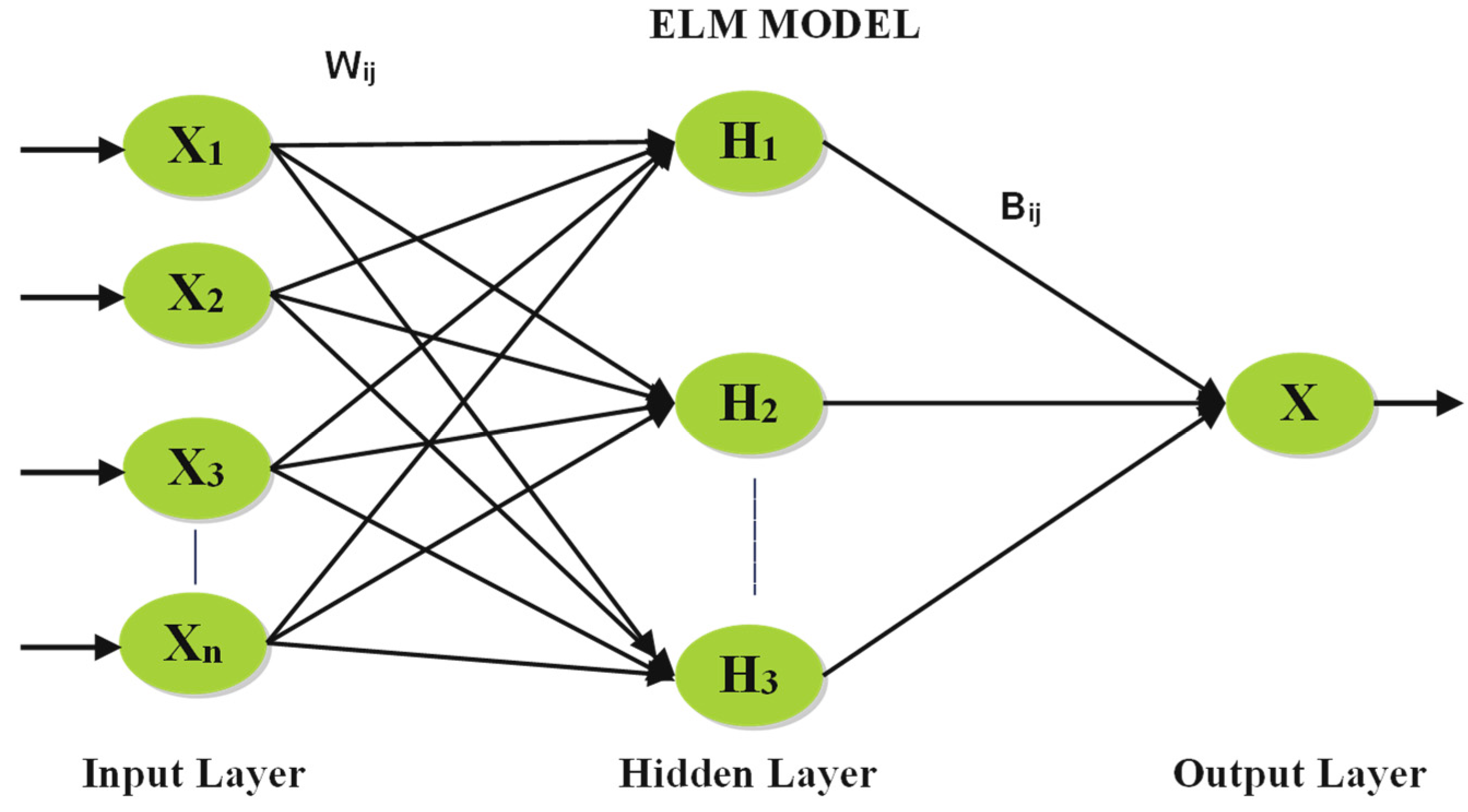
Here, H + represents the pseudo-inverse of H . The training process of ELM involves solving H β = T to determine the optimal output weights β , thereby minimizing the error between the model output Y i and the target T i . This direct, matrix-based approach makes ELM computationally efficient and suitable for modeling complex systems. ELM is illustrated in Figure 5.

3.2. ELM-PLSCO Model

PLSCO is employed to optimize the weights ( W ) and biases ( B ) of ELM, enhancing its predictive accuracy and robustness. In this model, PLSCO is utilized to identify the optimal parameters for ELM by iteratively refining the input weight matrix ( W ) and hidden bias vector ( B ) to minimize the error between the predicted output ( Y ) and the target values ( T ) . The integration of PLSCO ensures an adaptive and balanced search process, leveraging both exploration and exploitation. The process begins by initializing a population of high-energy particles, where each particle represents a candidate solution comprising randomly generated W and B values for the ELM. The fitness of each particle is evaluated using the accuracy metric, which measures the accuracy of the ELM output. The global best solution, X best , is identified based on the highest accuracy score.
In each iteration, the PLSCO framework divides the population into winners and losers through competitive learning. Winners, representing candidate solutions with better fitness, are updated using the PLO mechanism, which emphasizes exploitation. The PLO’s components, including gyration motion and auroral oval walks, refine the W and B values in high potential regions of the search space, ensuring precise adjustments for convergence. Conversely, losers are updated using the SSA, which focuses on exploration. The SSA encourages global search by directing particles to unexplored areas, preventing premature convergence, and maintaining population diversity. After updating the positions of winners and losers, the fitness of each particle is re-evaluated using the outcomes of the ELM predictions. Particles are selectively updated, retaining new positions if fitness improves; otherwise, previous positions are maintained. The global best solution, X best , is dynamically updated whenever better fitness is achieved. This iterative process continues until the maximum number of iterations M a x t is reached. By integrating PLSCO into the ELM framework, the optimization process benefits from an adaptive balance between local exploitation and global exploration, ensuring efficient and accurate tuning of W and B . This combination enhances the ELM’s ability to model complex systems, reduces the risk of overfitting, and achieves higher prediction accuracy compared to conventional optimization methods. The flowchart of ELM-PLSCO is illustrated in Figure 6.

4. Experiment and Discussion

4.1. Analysis of PLSCO Search Capability

In this section, the performance of the proposed optimization algorithm is evaluated and compared against existing and improved algorithms prior to its application to the predictive maintenance problem. The evaluation is conducted using two established benchmark function suites: CEC2015 and CEC2020. The experimentation and analyses employ the CEC2015 test suite to assess the algorithm’s capabilities. This suite comprises single-modal functions (F1–F2), multimodal functions (F3–F5), hybrid functions (F6–F8), and composite functions (F9–F15) [44]. Similarly, the CEC2020 test suite includes F16 (single modal functions), F17–F19 (basic multimodal functions), F20–F22 (hybrid functions), and F23–F25 (composition functions) [45]. The parameter settings for each algorithm are detailed in Table 2. Other key experimental parameters include a maximum of 2000 iterations, 30 independent runs, a problem dimension of 30, and a population size of 30. The proposed algorithm is compared with several state-of-the-art optimization algorithms: Adaptive Chaotic Gaussian RIME optimizer (ACGRIME) [46], Aquila Optimizer (AO) [47], African Vulture Optimization Algorithm (AVOA) [48], Opposition Based Learning Path Finder Algorithm (OBLPFA) [49], PathFinder Algorithm (PFA) [50], Parrot Optimizer (PO) [51], Pelican Optimization Algorithm (POA) [52], Sine Cosine Algorithm (SCA) [53], and Polar Light Optimizer (PLO) [38]. It is noteworthy that within this study, the comparative experiments incorporated an improved recent optimizer, such as ACGRIME and OBLPFA, as a representative hybrid and enhanced optimizer. While other optimizers, such as AO, AVOA, PFA, POA, SCA, and PLO represent recent and original optimizers, PLSCO is distinct in its cooperative competition mechanism, where winners are refined using PLO’s exploitation dynamics and losers explore via SSA’s leader–follower strategy. This structure, combined with adaptive parameter adjustment, enables a dynamic balance between exploration and exploitation throughout the optimization process.

4.1.1. Analysis of CEC 2015

In the experiments conducted using the CEC2015 test functions, two key metrics were evaluated: the Average (AVG) and Standard Deviation (STD) of results, as presented in Table 3. The unimodal functions selected for this study were specifically used to assess the exploitation capabilities of the algorithms. The results indicate that for the test function F1, the proposed PLSCO achieved the lowest mean value, outperforming all compared algorithms. However, for F2, ACGRIME demonstrated superior performance, while algorithms such as AO, PO, POA, and SCA exhibited subpar performance in these functions. For the multimodal functions (F3–F5), PLSCO consistently outperformed other algorithms in terms of average values, highlighting its superior accuracy in addressing multimodal optimization problems. An exception is observed in F5, where PLSCO achieved results similar to POA, which remained the most accurate optimizer among the comparisons. In the hybrid function tests (F6–F8), PLSCO exhibited varying performance. While it was less accurate than ACGRIME for F6, it achieved better mean values and greater stability, as reflected in lower standard deviations for F7 and F8. These results underscore the improved capability of PLSCO to handle hybrid problems with diverse characteristics effectively. The improvement of ACGRIME in F2 and F6 is attributed to ACGRIME’s enhanced optimization ability in specific unimodal landscapes and hybrid functions with narrow optima, where its adaptive chaotic perturbations provide improved precision. Also, according to the no free lunch theorem, no single algorithm can be efficient for all optimization problems [54]. For composite functions (F9–F15), PLSCO demonstrated outstanding performance, particularly in F11, F13, F14, and F15, achieving solutions closest to the global optimum compared to other algorithms. These results validate the algorithm’s robust ability to optimize complex, high-dimensional problems with composite structures.
The experimental results with the CEC2015 test functions demonstrate that PLSCO consistently performs well across unimodal, multimodal, hybrid, and composite functions. This superior performance can be attributed to the integration of SSA operators, which enhance the algorithm’s exploration capabilities by encouraging global search and maintaining diversity within the population. Additionally, the competitive learning framework plays a crucial role in dynamically balancing exploration and exploitation by classifying particles into winners and losers. Winners refine their solutions through the PLO mechanism, which emphasizes precise local search, while losers adopt the SSA approach to explore unvisited regions, preventing premature convergence. The synergy between CSO’s competitive learning and SSA operators ensures that PLSCO effectively navigates complex search spaces and adapts to the characteristics of diverse optimization problems. These findings underscore PLSCO’s potential as a robust, adaptive, and versatile optimization algorithm for solving a wide range of challenging optimization tasks.

4.1.2. Analysis of CEC2020

The experimental results presented in Table 4 for the CEC2020 benchmark functions demonstrate that PLSCO consistently obtained superior performance across various categories of optimization problems. For single-modal functions (F16), PLSCO achieved an average fitness value that significantly surpasses the traditional PLO, showcasing its enhanced exploitation capabilities. However, the best performance in F16 was achieved by the ACGRIME algorithm. In basic multimodal functions (F17–F19), PLSCO exhibited exceptional exploration abilities and resistance to local optima, particularly in F19, where it achieved the most optimal average fitness, matching the performance of the improved algorithm ACGRIME. While the performance of PLSCO in F17 and F18 was slightly lower than that of ACGRIME, it demonstrated a competitive capability to navigate multimodal landscapes effectively.
The results for hybrid functions (F20–F22) further underscore PLSCO’s adaptability and robustness. PLSCO outperformed other algorithms, such as PO and PFA, in terms of average fitness across F20–F22. Additionally, its relatively low standard deviation reflects a high degree of stability and reliability, further establishing its superiority over competing methods, including recently developed algorithms like POA. For composition functions (F23–F25), PLSCO showcased its ability to maintain an effective balance between exploration and exploitation. It consistently achieved the best average fitness in these functions, outperforming not only improved algorithms such as ACGRIME and OBLPFA but also recently proposed methods like AVOA and PO. These results highlight PLSCO’s capacity to converge rapidly while effectively exploring complex, high-dimensional solution spaces. The results in Table 4 emphasize PLSCO’s superior optimization performance, robustness, and stability across all function categories. By integrating advanced strategies, including competitive learning and SSA operators, PLSCO achieves a dynamic balance between exploration and exploitation, leading to improved convergence rates, enhanced exploratory capabilities, and better overall performance compared to competing algorithms. These findings firmly establish PLSCO as a versatile and reliable optimization algorithm for tackling a wide range of challenging problems.

4.1.3. Convergence and Box Plot Analysis

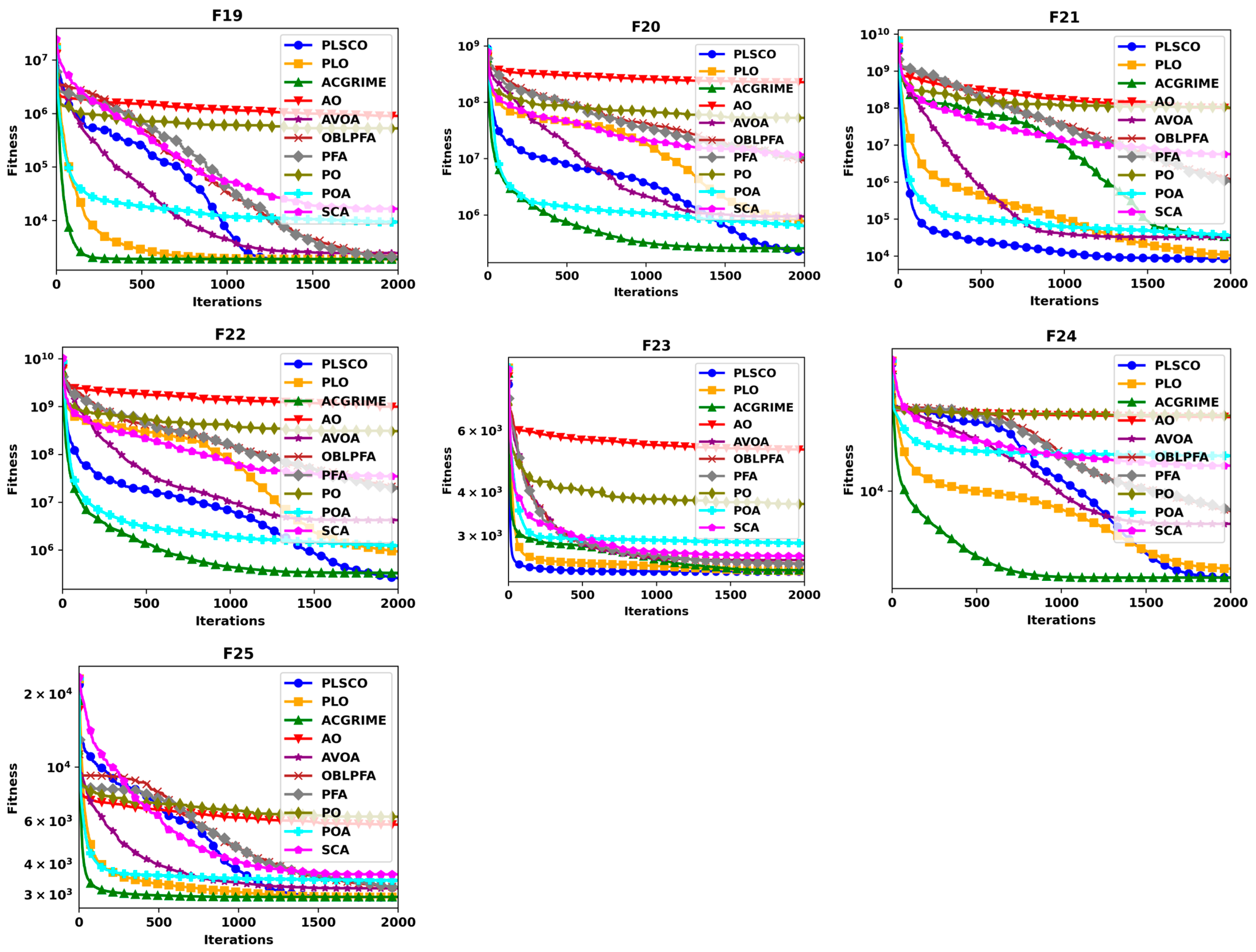
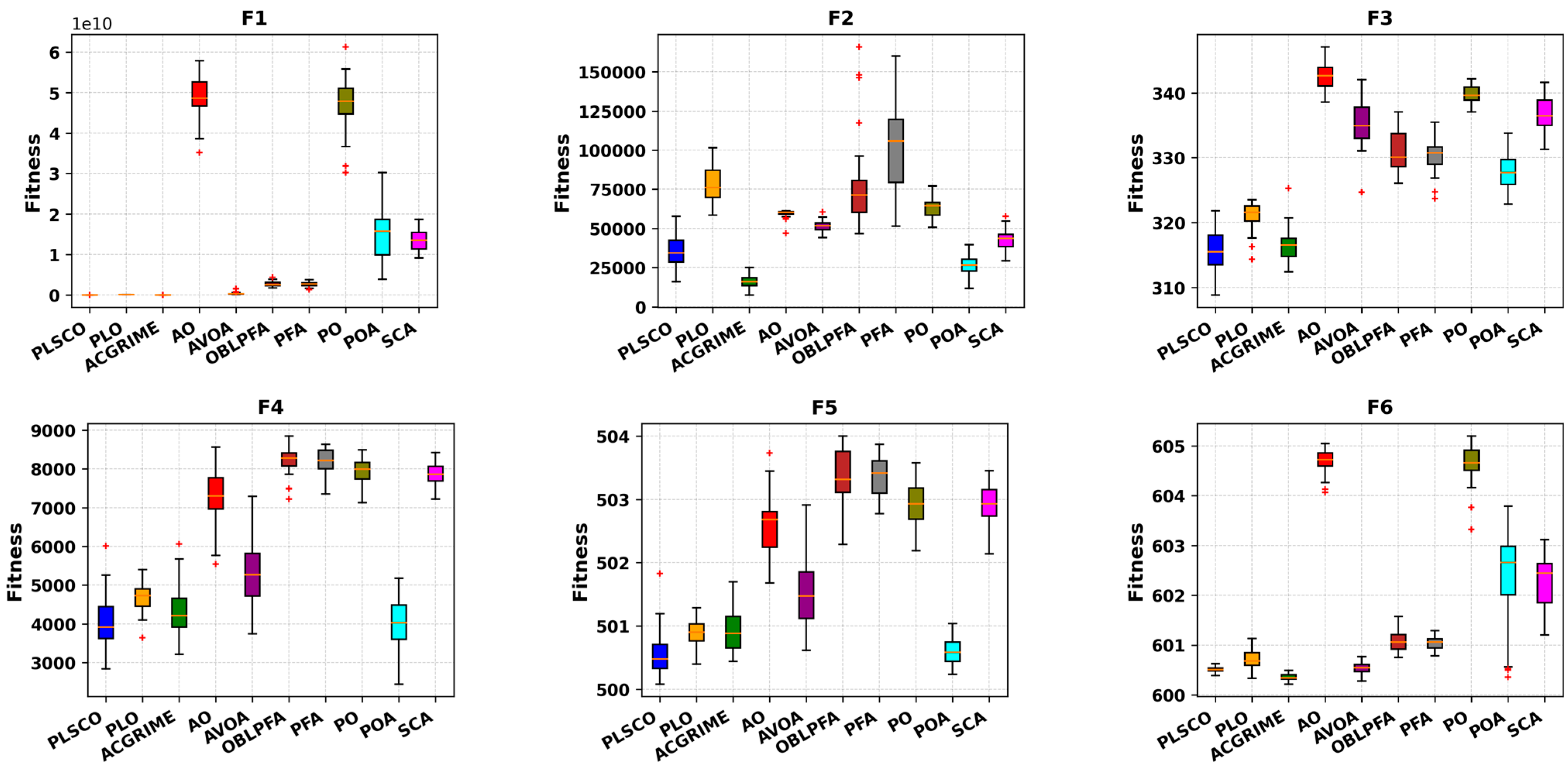
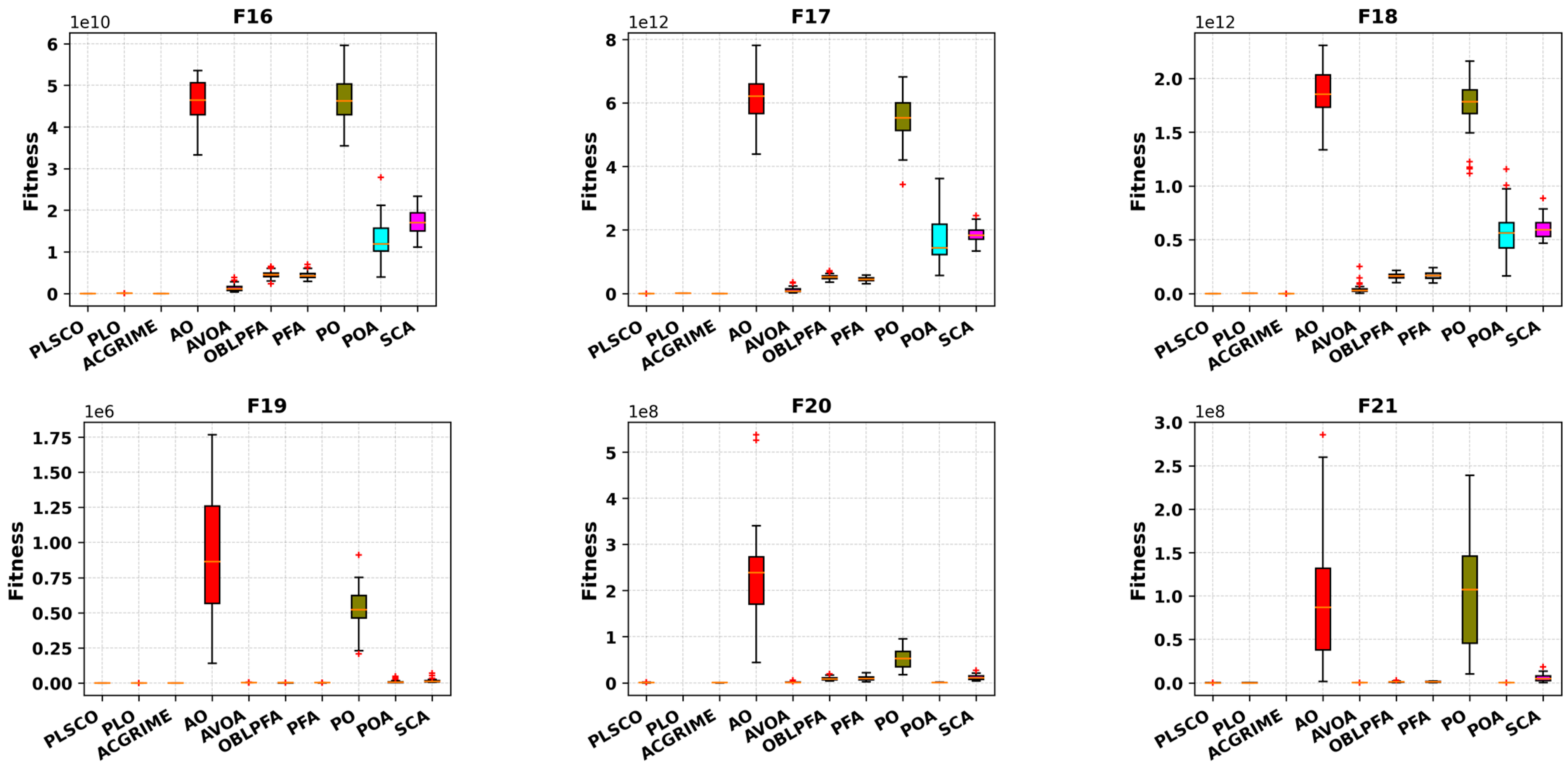
Figure 7, Figure 8, Figure 9 and Figure 10 present a comparative analysis of the PLSCO method against nine state-of-the-art algorithms using convergence curves and box plots on the CEC2015 and CEC2020 benchmark functions, respectively. The convergence curves, depicted in Figure 7 and Figure 8, illustrate how the average accuracy of each algorithm evolves as the number of iterations increases. The box plots in Figure 9 and Figure 10 provide a detailed view of the distribution of final optimal solutions attained by each algorithm. These plots display critical statistical elements, including the minimum, maximum, lower quartile (Q1), median, upper quartile (Q3), and any outliers, with outliers distinctly marked as red “+” symbols. While the convergence curves evaluate how effectively each algorithm achieves optimal solutions over iterations, the box plots highlight the stability and consistency of the results, with smaller box sizes indicating greater robustness against variations in the search space. The convergence curves demonstrate that PLSCO achieves rapid convergence in the early stages of the optimization process. Unlike other algorithms, which tend to exhibit flattened curves and stagnate in local optima, PLSCO continues to explore high-quality regions of the search space. Notably, PLSCO demonstrates faster convergence across all functions except F1 in the unimodal category (F1–F2), underscoring its effective exploitation capabilities. For multimodal functions (F3–F5), PLSCO delivers superior performance, achieving higher accuracy, particularly in F3 and F4, compared to other optimizers. In hybrid functions (F6–F8), PLSCO shows exceptional convergence for F6 and F8, with results comparable to other advanced algorithms, indicating its adaptability to diverse problem characteristics.
In composite functions F11 and F15, PLSCO surpasses advanced algorithms such as ACGRIME, OBLPFA, and PLO by maintaining an optimal balance between exploration and exploitation. The findings depicted in Figure 7 further validate PLSCO’s ability to achieve superior convergence accuracy compared to other techniques. This highlights the effectiveness of the enhancements introduced in PLSCO, which not only improve the trade-off between exploration and exploitation but also enhance its ability to avoid local optima and approach the global optimum with greater precision.
The integration of the SSA and CSO strategies within PLSCO is central to its superior performance. The competitive learning framework fosters diversity by dynamically classifying particles as winners and losers, encouraging both local refinement and global exploration. SSA operators ensure continuous exploration of the solution space, maintaining diversity and preventing premature convergence. Additionally, the methodological innovations in PLSCO enable it to excel in shifted, rotated, and hybrid functions within the CEC2020 benchmark, particularly in F20, F21, F22, F23, and F25, as shown in Figure 8. The box plot analyses in Figure 9 and Figure 10 further reinforce PLSCO’s stability, with tight distributions and minimal outliers, underscoring its robustness. The red “+” in the plots are outliers

4.1.4. Diversity Analysis

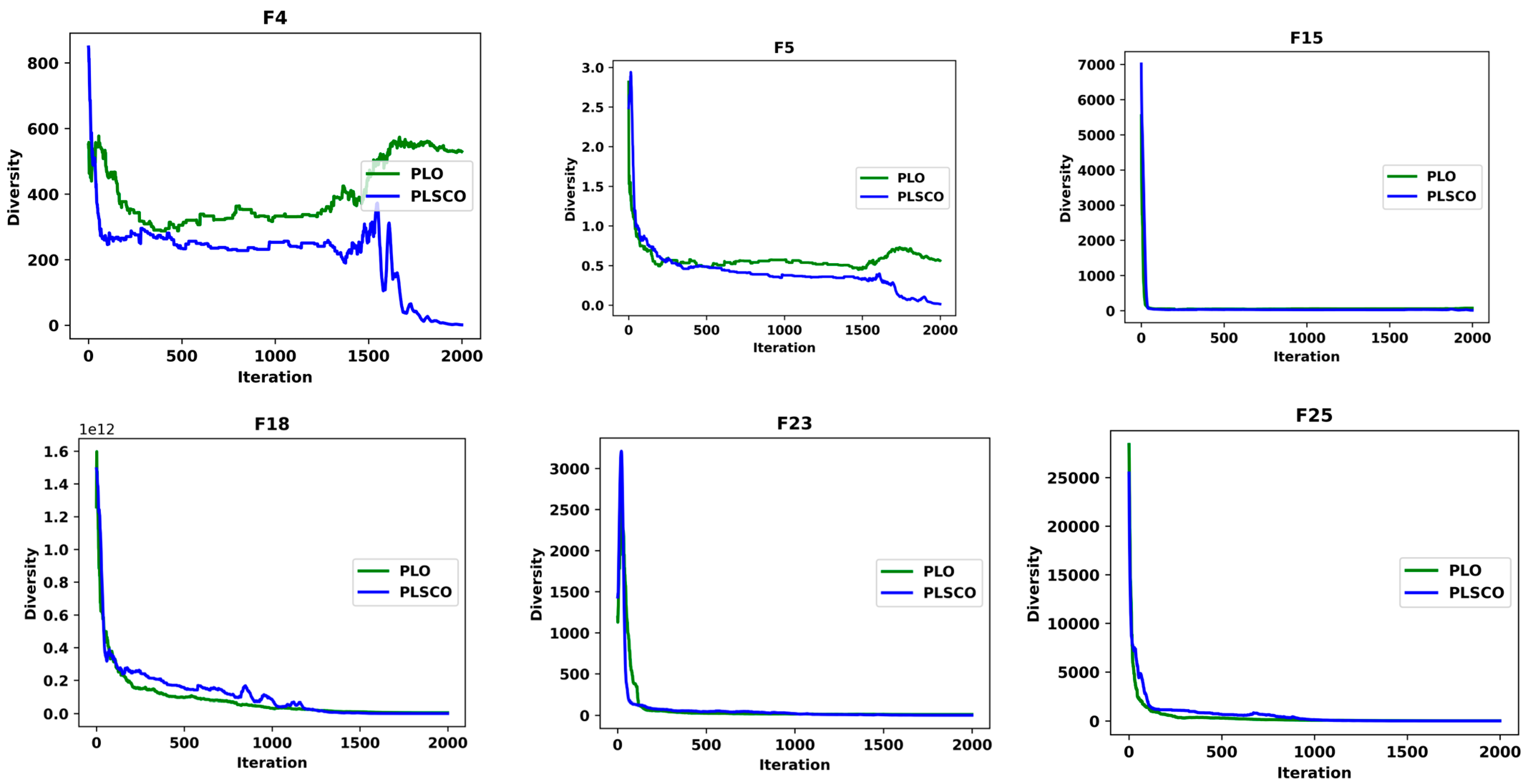
To emphasize the enhancements introduced by PLSCO over the standard PLO, a diversity analysis is conducted to evaluate the distribution of the population throughout the optimization process [55]. Population diversity captures the nonlinear dynamics of the population by measuring the average distance between individuals over iterations. A reduction in diversity, characterized by nonlinear behavior, suggests increased aggregation within the population, heightening the risk of premature convergence to suboptimal solutions. The population radius, defined as the maximum distance between any two individuals, is mathematically expressed in Equation (32) [56].
| D | = m a x ( i j ) [ 1 , | X | ]   t = 1 D     X i , t X j , t 2
where | X | is the population size, D is the dimensionality of the problem space, and X i , t represents the position of the i -th individual in the t -th dimension. From this, the diversity of the population is calculated as expressed in Equation (33).
D N = 1 | X | | D | i = 1 | X |   t = 1 D     X i , t X t 2
where X t denotes the center of the population. Figure 11 illustrates the diversity trajectory for selected benchmark functions, specifically F4, F5, and F15 from CEC2015 and F18, F23, and F25 from CEC2020. The results reveal that during the early stages of the optimization process, PLSCO exhibits significantly higher diversity compared to the standard PLO. This heightened diversity is attributed to the integration of SSA operators within PLSCO, which ensures a broad exploration of the search space by maintaining the dispersion of search agents. Consequently, this reduces the risk of premature convergence to suboptimal solutions, allowing for more effective global exploration.
In contrast, PLSCO demonstrates reduced population diversity in the later stages of the search compared to PLO. This indicates that the search agents in PLSCO have transitioned from global exploration to focused exploitation, progressively converging toward the global optimum. This behavior is driven by the CSO strategy, which dynamically refines the solutions by guiding the population to optimal regions while avoiding local optima. The interplay between SSA and CSO ensures a balanced and adaptive search process. SSA maintains diversity during the initial phases, enabling PLSCO to escape local optima and explore diverse regions of the solution space. CSO, on the other hand, enhances exploitation in the later stages, concentrating the search around high-potential areas and ensuring convergence to near-optimal solutions. This dynamic balance, as evidenced by the diversity trajectory analysis, underscores PLSCO’s superiority over PLO, enabling it to achieve higher optimization performance, robustness, and stability across a wide range of benchmark functions.

4.1.5. Exploration vs. Exploitation

This section presents the comprehensive analysis of PLSCO’s local and global search capabilities, focusing on its ability to balance exploration and exploitation; these are the two foundational components of optimization algorithms. The aim of evaluating the mathematical formulations and visual representations of these proportions is to assess PLSCO’s effectiveness in dynamically adapting its search strategies. The mathematical expressions for calculating exploration and exploitation proportions are expressed in Equations (34)–(37) [57].
D i v j = 1 | X | i = 1 | X |     m e d i a n X i , j t X i , j t
F D i v t = 1 D j = 1 D     D i v j
E R P = F D i v F D i v max   t
E T P = F D i v max   F D i v t F D i v max   × 100
Here, X i , j t represents the j -th element of the i -th agent in the population during the t -th iteration. The median function computes the median value of the matrix, reflecting central tendencies within the population. F D i v t measures the average difference in the population’s dimensions at the t -th iteration, while F D i v max   represents the maximum observed value of F D i v t . Exploration and exploitation proportions, denoted as ERP and ETP, respectively, are expressed as percentages, indicating the relative focus of the algorithm during each phase of the search.
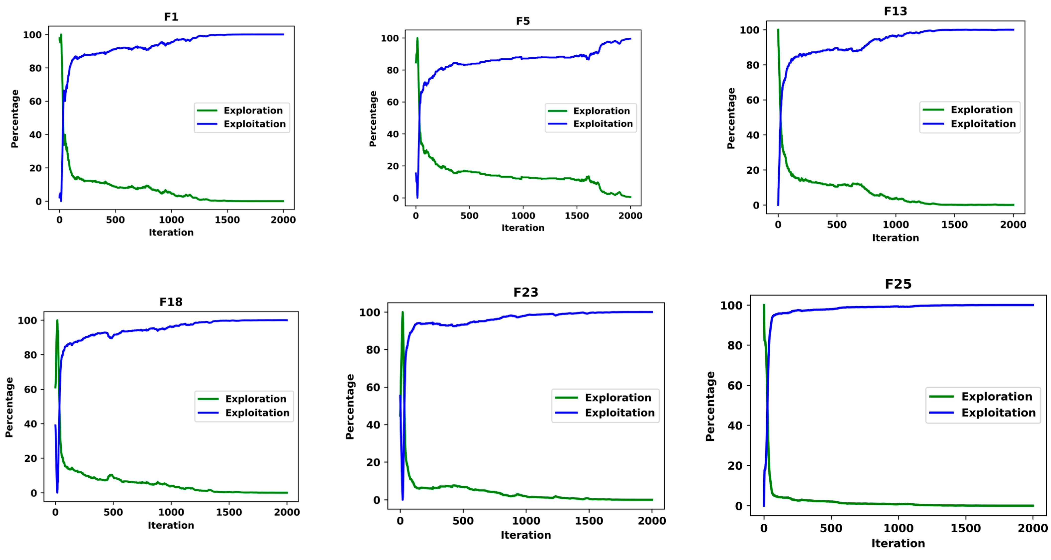
Figure 12 provides visual insights into the dynamics of exploration and exploitation rates for benchmark functions from CEC2015 ( F 1 , F 5 , and F 13 ) and CEC2020 ( F 18 , F 23 , and F 25 ). The curves illustrate PLSCO’s remarkable ability to adaptively balance these two phases across all agents during the optimization process. In the initial stages, the ERP is dominant, reflecting the algorithm’s emphasis on global exploration to investigate diverse regions of the solution space. As the search progresses, the ERP gradually decreases, allowing the ETP to predominate, signaling a shift toward refined exploitation of promising regions to identify optimal solutions. This adaptive behavior is attributed to the integration of the SSA and CSO within PLSCO. The SSA operators enhance global exploration in the early iterations by maintaining population diversity and preventing premature convergence. Meanwhile, the CSO strategy dynamically guides the search toward high-potential regions by refining local exploitation, particularly in later stages. These techniques orchestrate a seamless interplay between exploration and exploitation, enabling PLSCO to navigate complex optimization landscapes effectively.
The findings depicted in Figure 12 highlight PLSCO’s ability to maintain a dynamic equilibrium between exploration and exploitation, steering agents toward the global optimum. By emphasizing exploration in the initial phases and transitioning toward exploitation as the search progresses, PLSCO demonstrates its capability to adaptively balance these phases, resulting in efficient convergence and superior optimization performance. This methodological refinement positions PLSCO as a robust and versatile optimization algorithm capable of solving high-dimensional and complex problems with precision.

4.1.6. Non-Parametric Analysis

To ensure a rigorous evaluation of the experimental results and mitigate the impact of randomness, the outcomes of 30 independent iterations for each of the 10 algorithms across 25 test functions were analyzed using the Wilcoxon rank-sum test at a significance level of 0.05. This statistical test was employed to identify significant differences between the results of PLSCO and the comparison algorithms. A p-value greater than 0.05 indicates no significant difference between the results, whereas a p-value less than or equal to 0.05 signifies a statistically significant difference. The pairwise Wilcoxon rank-sum test results for PLSCO and the other algorithms are summarized in Table 5, with “-” denoting instances where no results were available for pairwise comparison.
The results from the CEC2015 and CEC2020 benchmark functions demonstrate that PLSCO exhibits significant differences compared to the majority of the evaluated algorithms, particularly the traditional PLO. This underscores the enhancements introduced in PLSCO, including the integration of SSA and CSO strategies, which contribute to its superior performance. In some cases, algorithms such as ACGRIME and POA achieved superior outcomes on specific test functions, resulting in p-values greater than 0.05, indicating comparable performance with PLSCO. However, in the majority of the benchmark functions, PLSCO achieved the best results, reaffirming its robustness and effectiveness in solving diverse optimization problems. Additionally, the Friedman Mean Rank Test was conducted to further validate the relative efficiency of the algorithms. PLSCO consistently obtained the highest mean rank across both the CEC2015 and CEC2020 test suites, establishing it as the most efficient algorithm among the compared methods. This performance can be attributed to the synergistic integration of SSA and CSO mechanisms, which ensure a dynamic balance between exploration and exploitation. The SSA strategy enhances global exploration by maintaining diversity and preventing premature convergence, while the CSO mechanism fosters local refinement, guiding the population toward optimal solutions in the later stages. These methodological advancements position PLSCO as a versatile and highly effective optimization algorithm capable of achieving superior performance across a wide range of challenging optimization landscapes.

4.2. Predictive Maintenance Prediction Using ELM-PLSCO Model

4.2.1. Dataset

In this study, the AI4I 2020 Predictive Maintenance Dataset from the UCI Machine Learning Repository was utilized [58]. This dataset was selected due to the challenges associated with acquiring predictive maintenance data from real-world industrial environments [59]. It provides a reliable representation of actual predictive maintenance scenarios encountered in industrial applications. The dataset comprises 10,000 data points with seven distinct features and a machine failure label, making it a robust resource for evaluating predictive maintenance models [60]. The features of the dataset are as follows:
  • Type: This categorical variable classifies products into three categories based on performance levels: high (H, representing 20% of all products), medium (M, representing 30% of all products), and low (L, representing 50% of all products).
  • Air Temperature: Measured in Kelvin (K), this feature is normalized to have a standard deviation of 2K centered around 300 K, reflecting the air temperature conditions during operations.
  • Process Temperature: Also measured in Kelvin (K), this feature is normalized with a standard deviation of 1K and represents the temperature within the machine’s operational processes.
  • Rotational Speed: Expressed in revolutions per minute (rpm), this value is calculated based on a machine power output of 2860 W, indicating the tool’s operational speed.
  • Torque: Measured in Newton meters (N m), torque values are distributed around 40 N m with a standard deviation of 10 N m, with no negative values recorded.
  • Tool Wear Time: This feature, measured in minutes, captures the cumulative operational time of the tool, representing its wear level over time.
  • Failure type: Machine failures are categorized into five distinct modes:
    i.
    Tool Wear Failure: Tool wear or replacement occurs randomly between 200 and 240 minutes of operation.
    ii.
    Heat Dissipation Failure: Failure occurs when the difference between air temperature and process temperature falls below 8.6 K, and the rotational speed drops below 1380 rpm.
    iii.
    Power Failure: This failure arises when the product of torque and rotational speed results in power exceeding 9000 W or dropping below 3500 W.
    iv.
    Overstrain Failure: Overstrain occurs when the product of torque and tool wear exceeds specified thresholds for each product category: 11,000 min N m for L products, 12,000 min N m for M products, and 13,000 min N m for H products.
    v.
    Random Failure: Failures that occur randomly with a probability of 0.1%, irrespective of process parameters.
The diverse and complex characteristics of the dataset make it an ideal benchmark for evaluating the performance of predictive maintenance models. By integrating PLSCO with ELM, the weight and bias parameters of ELM are optimized to enhance its predictive accuracy for identifying machine faults. The detailed feature set and failure labels enable comprehensive testing of PLSCO’s capability to balance exploration and exploitation, ensuring ELM effectively learns and generalizes across diverse failure scenarios. In this dataset, failure type is used as the target variable, while others are used as the input variables in a predictive model. Although the AI4I 2020 dataset provides a robust and well-structured platform for evaluating predictive maintenance models, it does not fully replicate the noise levels, class imbalance, and heterogeneous data distributions encountered in real industrial environments. The selection of this dataset was driven by the limited availability of publicly accessible PdM datasets with comprehensive feature sets and accurate labeling. Nonetheless, the proposed PLSCO-ELM framework incorporates features such as competitive learning and adaptive parameter adjustment that are suited to handle variability and noise in more complex datasets.

4.2.2. Evaluation Metrics

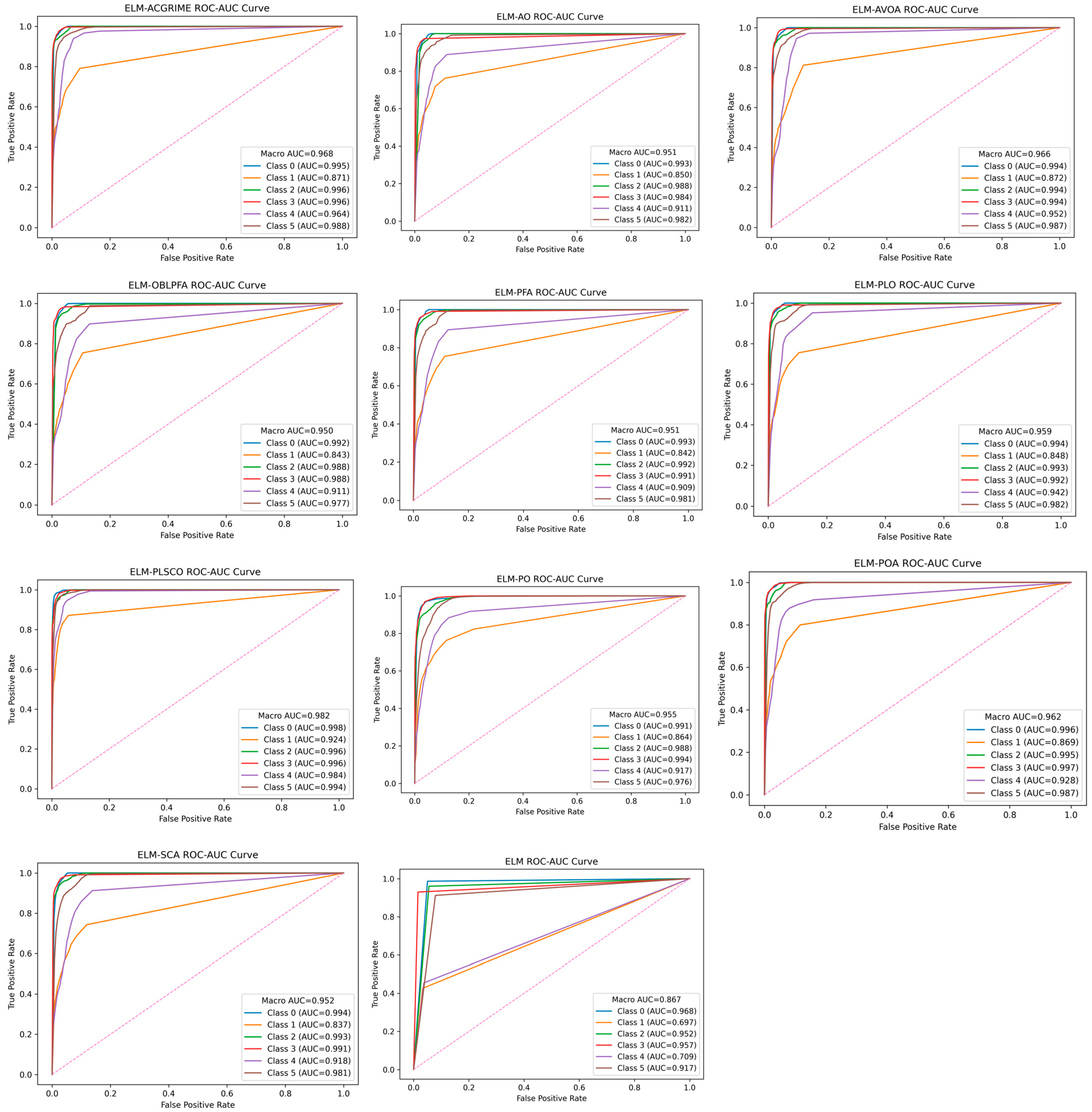
The evaluation criteria used to assess the performance of the PLSCO-enhanced ELM are summarized in Table 6. They provide a comprehensive framework for evaluating the model’s predictive accuracy and reliability. Aside from the metrics in the table, the Area Under the Receiver Operating Characteristic Curve (ROC-AUC) is included in the metrics. It reflects the classifier’s ability to discriminate between different classes, and is a performance metric derived from the ROC curve. The interpretation of ROC-AUC scores is generally as follows: 0.5–0.6 indicates poor or failed classification performance, 0.6–0.7 suggests a weak or marginal level of class separability, 0.7–0.8 indicates fair performance, 0.8–0.9 indicates considerable or good discrimination, and above 0.9 indicates excellent classification ability [61].
These metrics are critical for understanding the effectiveness of the optimized ELM in identifying machine faults within the PdM dataset. By employing these evaluation criteria, the effectiveness of PLSCO in optimizing ELM’s weights and biases can be rigorously assessed. These metrics ensure a thorough evaluation of the model’s ability to identify machine faults accurately and reliably, highlighting the enhancements brought about by the integration of PLSCO into the predictive maintenance framework.

4.2.3. Prediction Results and Discussion

In this section, the parameters for all optimization algorithms are maintained as specified in Table 2. The number of iterations is set to 100, and the population size is fixed at 30 for all optimization algorithms utilized in this study. The search boundaries for PLSCO and the comparison algorithms in optimizing the weights and biases of ELM are defined within the range of [−10,10]. The hidden layer of ELM is configured with 15 neurons across all optimization algorithms employed in this study. The AI4I 2020 dataset was partitioned into training and testing sets using a randomized 70:30 split. To ensure that performance evaluations were robust to variability arising from random data partitioning, the performance metrics presented in Table 7 and Table 8 correspond to the average, standard deviation, and best performance, providing a statistically reliable measure of predictive accuracy and stability. In this study, the number of hidden layer neurons in ELM was fixed at 15. This choice aligns with existing applications of ELM, where similar configurations have demonstrated a favorable trade-off between model complexity and generalization capability, while mitigating overfitting risks [62]. Given that the central focus of this work is to evaluate the impact of PLSCO on the optimization of ELM’s weights and biases, the number of neurons is kept constant to ensure that observed performance differences stem directly from the optimization mechanism rather than architecture variability. The results of the experiment demonstrate that the improved PLSCO significantly enhances the predictive performance of ELM in identifying machine faults more accurately from the dataset compared to other nature-inspired optimization techniques. The performance of the algorithms was assessed using several metrics across both training and testing datasets, as seen in Table 7 and Table 8. PLSCO consistently outperformed its counterparts, achieving the highest average accuracy of 0.95682 for training and 0.95465 for testing, respectively, and recall of 0.86951 for training and 0.86587 for testing, respectively, alongside superior F1, precision, and specificity. This exceptional performance underscores the algorithm’s robustness and effectiveness in optimizing the ELM model for PdM tasks.
When compared to other algorithms, such as ACGRIME, AO, AVOA, and POA, PLSCO demonstrated a clear advantage in accuracy, as evidenced by its score. As seen in Table 8, PLSCO’s accuracy score is superior to competing algorithms, indicating a high degree of reliability. A deeper analysis of the performance metrics reveals that while most algorithms demonstrated high specificity, there was a trade-off in terms of precision and F1 score for several methods. However, PLSCO achieved the highest specificity (0.97409 for training and 0.97280 for testing) and maintained a balanced and superior performance across precision and F1 score, reflecting its capability to minimize false positives while accurately identifying true machine faults. This balance is crucial for predictive maintenance applications, where both overestimating and underestimating machine faults can lead to operational inefficiencies or unexpected downtimes.
The consistency and stability of PLSCO’s performance are further reinforced by its low standard deviations across all metrics. Also observed in the ROC-AUC average score, PLSCO demonstrated superior performance with an average test score of 0.97224, indicating that it can discriminate effectively within the classes of the predicted value. However, ELM demonstrated even better standard deviations for all metrics. This superior standard deviation in ELM is attributed to its deterministic nature in training, stemming from the direct computation of output weights using the Moore-Penrose pseudo-inverse. Unlike iterative optimization-based methods, such as PLSCO, where performance may be slightly influenced by randomness in population initialization and search trajectories, ELM’s matrix-based approach ensures minimal variability across multiple runs. Consequently, this characteristic contributes to ELM’s exceptionally stable performance, particularly in scenarios requiring repeated trials or consistent outcomes. This stability is particularly evident in scenarios involving noisy or imbalanced data, where other algorithms may struggle to maintain reliability. The results indicate that PLSCO’s design effectively addresses these challenges, making it a robust choice for real-world predictive maintenance tasks. Additionally, the algorithm’s ability to outperform the baseline ELM model by a significant margin underscores the importance of integrating advanced optimization techniques for enhancing machine learning models.
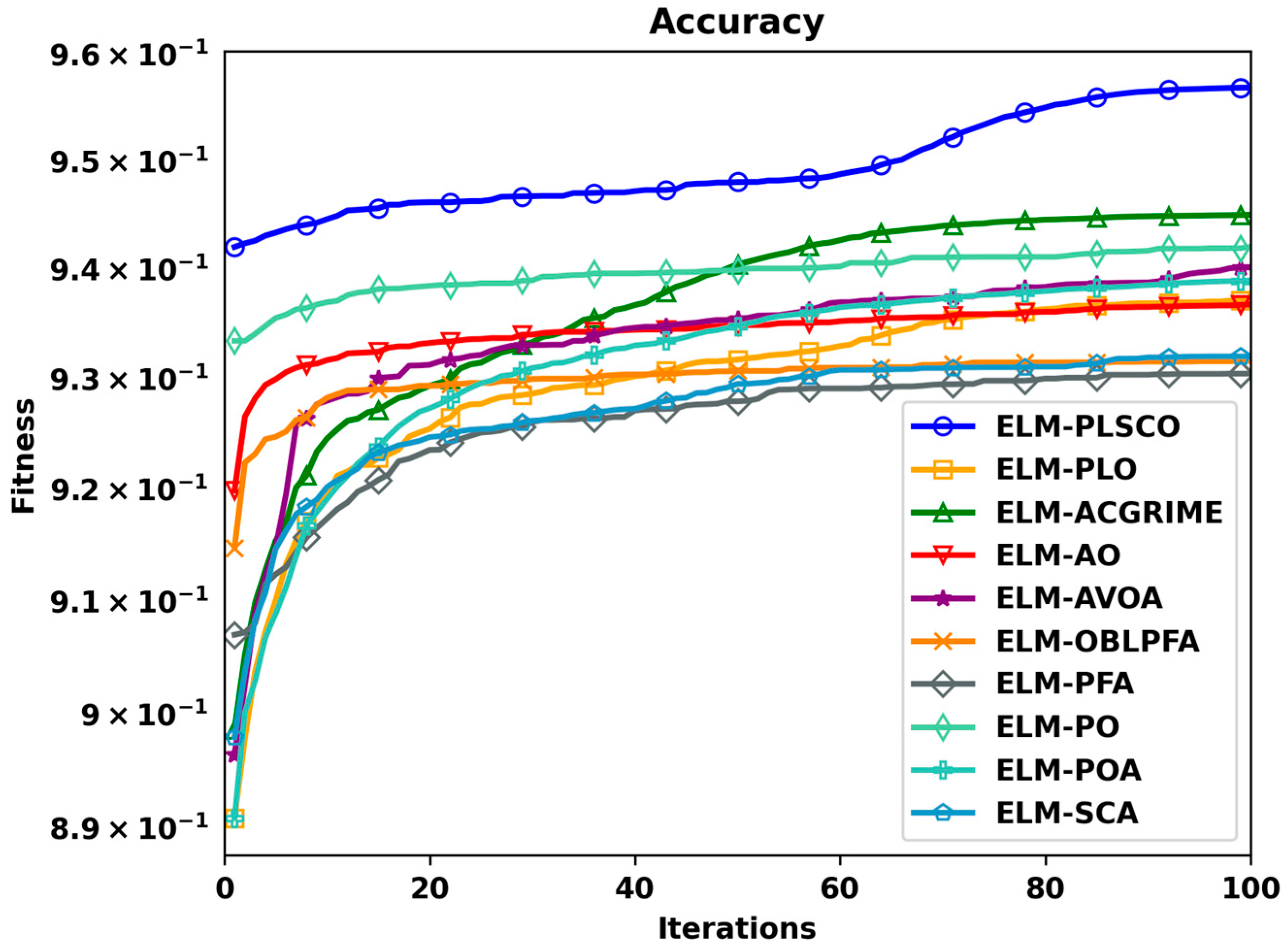
Furthermore, the convergence behavior, as depicted in Figure 13, illustrates the superior fitness and rapid stabilization of PLSCO relative to other optimization methods. Unlike competing algorithms, which exhibited slower or suboptimal convergence patterns, PLSCO achieved higher fitness values with fewer iterations, further validating its efficacy in enhancing the ELM-PLSCO model’s learning process. The plot provides valuable insights into their optimization performance. The fitness values for PLSCO are consistently higher throughout the iterations, clearly demonstrating its ability to quickly adapt and achieve optimal solutions. In contrast, other algorithms, such as AO and AVOA, exhibit slower convergence rates, requiring more iterations to approach fitness levels that are still below those achieved by PLSCO. Notably, PLSCO’s convergence curve shows a smooth and steady ascent, highlighting its efficiency in navigating the solution space without being hindered by local optima. This is a critical advantage in predictive maintenance applications, where timely and accurate predictions are essential for minimizing downtime and optimizing operational efficiency. The superior convergence behavior of PLSCO also suggests its potential applicability in other complex optimization scenarios.
The results highlight the transformative impact of using the PLSCO algorithm for optimizing ELM in PdM prediction. The algorithm’s ability to achieve superior accuracy, stability, and convergence speed positions it as a highly effective tool for enhancing machine fault prediction. The comparative analysis and convergence trends underscore its advantages over other nature-inspired algorithms, providing a strong case for its adoption in industrial settings. These findings demonstrate the potential of integrating advanced nature-inspired optimization techniques into predictive maintenance frameworks, paving the way for more reliable and efficient industrial applications.
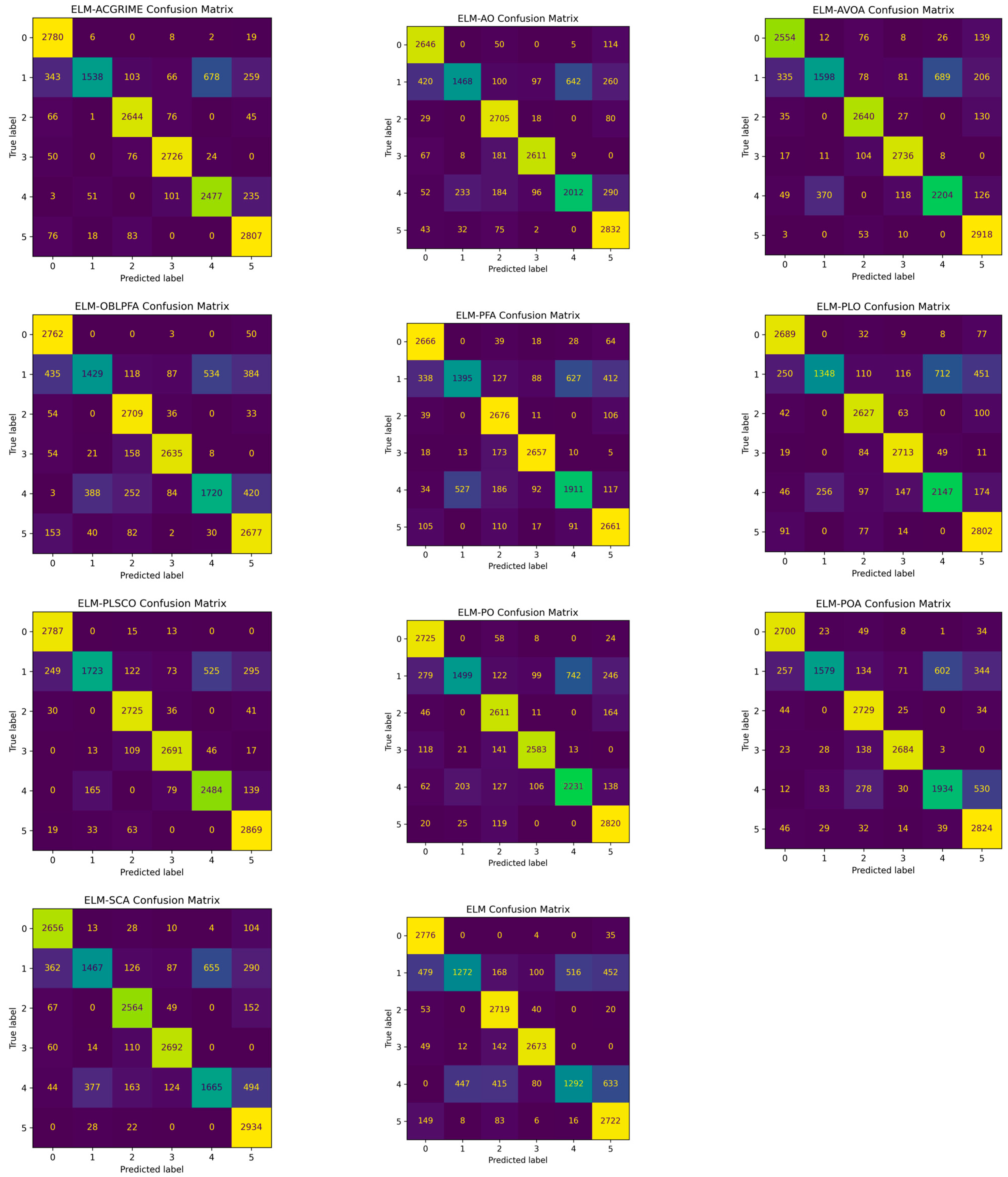
The confusion matrix plots of the best test accuracy from 30 independent runs are shown in Figure 14, confirming that ELM-PLSCO maintains a high true positive rate while minimizing false classifications, indicating its suitability for predictive maintenance tasks where fault detection accuracy is critical. Furthermore, the corresponding ROC–AUC plots of the best test accuracy from 30 independent runs are shown in Figure 15, illustrating that ELM-PLSCO consistently attains higher area under the curve values compared to other models, reflecting its robust discriminative capability under varying decision thresholds. This improvement can be attributed to the synergy of PLO’s competitive dynamics, CSO’s stochastic search diversity, and SSA’s adaptive exploitation, which collectively enhance the optimizer’s ability to balance exploration and exploitation. These findings suggest that the hybridization strategy not only accelerates convergence but also strengthens classification stability.
The computation time in seconds results presented in Table 9 reveal notable differences among the ELM-based hybrid optimization models. The proposed ELM-PLSCO achieved a moderate computation time of 287.21 seconds, which is competitive given its enhanced exploration–exploitation balance and improved convergence characteristics, which is higher than baseline ELM-PLO. While algorithms such as ELM-SCA and ELM-AVOA demonstrated the lowest computation times, their reduced runtime comes at the cost of lower predictive accuracy in earlier evaluations. Conversely, models such as ELM-PO and ELM-POA exhibited substantially longer runtimes, largely due to their more complex update strategies and less efficient convergence behavior. The ELM baseline, with a computation time of only 3.37 seconds, remains the fastest; however, it lacks the optimization capacity to fine-tune parameters effectively, leading to inferior predictive performance. The results indicate that ELM-PLSCO provides a favorable trade-off between computational efficiency and prediction accuracy, making it suitable for predictive maintenance applications where both accuracy and timeliness are critical.

4.2.4. Feature Importance Score Analysis

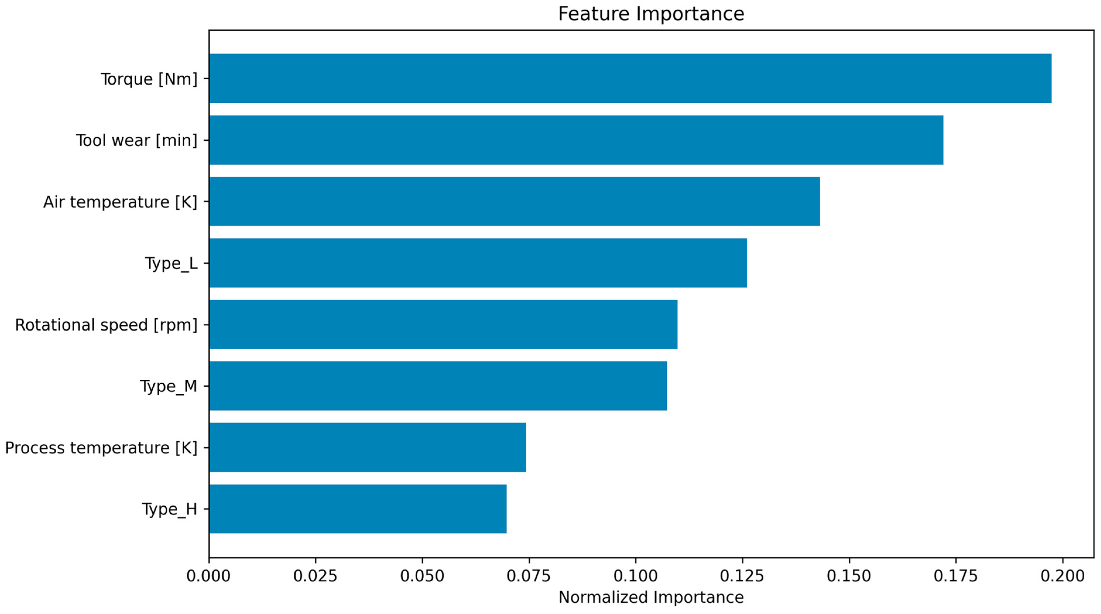
The feature importance analysis provides crucial insights into the predictive power of individual variables in the dataset for machine failure prediction. Feature importance was evaluated using the permutation importance score method, which assesses the decrease in model performance when the values of a given feature are randomly shuffled while all others remain unchanged. A greater drop in performance indicates a higher importance of that feature to the model’s predictions. As evident in Figure 16, torque emerges as the most significant feature, with the highest importance score. This indicates that torque plays a pivotal role in determining machine health, as variations in torque could directly reflect changes in mechanical load and operational efficiency. Following closely are tool wear and air temperature, both of which exhibit substantial contributions to the prediction model. The high importance of tool wear is expected, given its direct relationship to equipment degradation, while air temperature highlights the impact of environmental conditions on machine performance. The feature Type_L demonstrates a comparable level of importance. This is due to the inherent characteristics or operational conditions associated with these products, such as lower thresholds for durability or higher susceptibility to wear and tear. Rotational speed and Type_M exhibit moderate contributions, emphasizing their role in reflecting operational conditions.
In contrast, features such as process temperature and Type_H demonstrate lower importance, indicating they contribute less predictive power to the model’s predictions. Their relatively lower influence may stem from weaker correlations with the target variable or redundancy with other features. When combined with the performance metrics from the improved ELM-PLSCO algorithm, the feature importance analysis underscores the effectiveness of leveraging domain-specific insights for model optimization. The prioritization of features such as torque and tool wear validates the practical relevance of the proposed approach. Moreover, the hierarchical ranking of features highlights potential areas for targeted monitoring and intervention in real-world maintenance practices.
The findings from the feature importance analysis also complement the accuracy trends observed in the optimization algorithms’ fitness plots. Specifically, the ability of ELM-PLSCO to achieve superior performance could be attributed, in part, to its capability to better capture the relationships among these influential features. This synergy between feature importance and algorithmic performance demonstrates the potential for ELM-PLSCO to uncover meaningful patterns in complex datasets, ultimately driving advancements in predictive maintenance.

5. Conclusions

This study proposes an advanced PdM model that integrates the ELM with an enhanced optimization algorithm, termed PLSCO. PLSCO is developed by synergistically combining mechanisms from the CSO and the SSA within the PLO framework. This hybridization effectively addresses the critical challenge of balancing exploration and exploitation in optimization processes. A novel competitive division mechanism enables adaptive learning, enhancing both local refinement and global search capabilities, thereby significantly improving the overall optimization performance of the algorithm. The ELM-PLSCO model was evaluated on the AI4I 2020 Predictive Maintenance dataset, where it demonstrated superior predictive accuracy and stability compared to baseline ELM and conventional optimization-based approaches. Feature importance analysis revealed that variables such as torque and tool wear play a pivotal role in fault prediction, while product type and other operational parameters provide insights into performance-specific vulnerabilities. These findings highlight the model’s ability to extract meaningful and actionable knowledge from industrial data.
Despite its promising results, this study has several limitations. First, the evaluation was conducted using only a single publicly available dataset, the AI4I 2020 dataset, due to the limited availability of industry-reported PdM datasets in the public domain. Industrial predictive maintenance data are often proprietary and protected by confidentiality agreements, restricting access for research purposes. While the AI4I 2020 dataset offers a well-structured and balanced benchmark for controlled experimentation, it may not fully capture the complexities of real-world industrial environments, such as high noise levels, severe class imbalance, and heterogeneous operational conditions. Second, although the hybrid PLSCO algorithm exhibits strong optimization performance, its computational complexity in large-scale or real-time applications requires further investigation, as it requires more computation time. The scalability and efficiency of the algorithm under dynamic operational conditions warrant deeper analysis.
Future research will address these limitations by extending the proposed framework to dynamic, real-time environments and evaluating its performance across multiple PdM datasets obtained through industrial collaborations. This will enable a more comprehensive assessment of the model’s generalization capability across diverse industrial domains. Additionally, future work will incorporate domain-specific constraints and real-world operational dynamics into the optimization process to further improve the robustness and practical applicability of the model. Further experimental evaluations will include comparisons with other high-performance hybrid optimizers and emerging metaheuristic–machine learning integration techniques. The framework will also be systematically evaluated with respect to neuron count variation and different dataset partitioning strategies to identify optimal configurations and enhance model reliability.

Author Contributions

A.R.M.A.B., Methodology, Validation; O.S.O. writing—original draft preparation, supervision; T.O. Resources, Supervision and Editing: O.A. Conceptualization, Writing, Methodology, Validation. All authors have read and agreed to the published version of the manuscript.

Funding

This research received no external funding.

Institutional Review Board Statement

This study did not involve human participants, animals, or data requiring ethical review.

Informed Consent Statement

No human subjects were involved, and as such, no informed consent was required for this study.

Data Availability Statement

The data obtained through the experiments are available upon request from the corresponding author.

Conflicts of Interest

The authors declare no conflicts of interest.

References

  1. Nunes, P.; Santos, J.; Rocha, E. Challenges in predictive maintenance—A review. CIRP J. Manuf. Sci. Technol. 2023, 40, 53–67. [Google Scholar] [CrossRef]
  2. Ahmad, R.; Kamaruddin, S. An overview of time-based and condition-based maintenance in industrial application. Comput. Ind. Eng. 2012, 63, 135–149. [Google Scholar] [CrossRef]
  3. Bouabdallaoui, Y.; Lafhaj, Z.; Yim, P.; Ducoulombier, L.; Bennadji, B. Predictive Maintenance in Building Facilities: A Machine Learning-Based Approach. Sensors 2021, 21, 1044. [Google Scholar] [CrossRef]
  4. Abidi, M.H.; Mohammed, M.K.; Alkhalefah, H. Predictive Maintenance Planning for Industry 4.0 Using Machine Learning for Sustainable Manufacturing. Sustainability 2022, 14, 3387. [Google Scholar] [CrossRef]
  5. A Survey of Predictive Maintenance: Systems, Purposes and Approaches. Available online: https://www.researchgate.net/publication/337971929_A_Survey_of_Predictive_Maintenance_Systems_Purposes_and_Approaches (accessed on 21 January 2025).
  6. Hamasha, M.; Bani-Irshid, A.H.; Almashaqbeh, S.; Shwaheen, G.; Qadri, L.; Shbool, M.; Muathen, D.; Ababneh, M.; Harfoush, S.; Albedoor, Q.; et al. Strategical selection of maintenance type under different conditions. Sci. Rep. 2023, 13, 15560. [Google Scholar] [CrossRef] [PubMed]
  7. Carvalho, T.P.; Soares, F.A.A.M.N.; Vita, R.; Francisco, R.d.P.; Basto, J.P.; Alcalá, S.G.S. A systematic literature review of machine learning methods applied to predictive maintenance. Comput. Ind. Eng. 2019, 137, 106024. [Google Scholar] [CrossRef]
  8. Theissler, A.; Pérez-Velázquez, J.; Kettelgerdes, M.; Elger, G. Predictive maintenance enabled by machine learning: Use cases and challenges in the automotive industry. Reliab. Eng. Syst. Saf. 2021, 215, 107864. [Google Scholar] [CrossRef]
  9. Vithi, N.L.; Chibaya, C. Advancements in Predictive Maintenance: A Bibliometric Review of Diagnostic Models Using Machine Learning Techniques. Analytics 2024, 3, 493–507. [Google Scholar] [CrossRef]
  10. Hearst, M.A.; Dumais, S.T.; Osuna, E.; Platt, J.; Scholkopf, B. Support vector machines. IEEE Intell. Syst. Their Appl. 1998, 13, 18–28. [Google Scholar] [CrossRef]
  11. Zhang, Z. Introduction to machine learning: K-nearest neighbors. Ann. Transl. Med. 2016, 4, 218. [Google Scholar] [CrossRef]
  12. Grossberg, S. Recurrent Neural Networks. Scholarpedia 2013, 8, 1888. [Google Scholar] [CrossRef]
  13. Costa, V.G.; Pedreira, C.E. Recent advances in decision trees: An updated survey. Artif. Intell. Rev. 2023, 56, 4765–4800. [Google Scholar] [CrossRef]
  14. Friedman, N.; Geiger, D.; Goldszmidt, M. Bayesian Network Classifiers. Mach. Learn. 1997, 29, 131–163. [Google Scholar] [CrossRef]
  15. Hochreiter, S.; Schmidhuber, J. Long Short-Term Memory. Neural Comput. 1997, 9, 1735–1780. [Google Scholar] [CrossRef] [PubMed]
  16. Gu, J.; Wang, Z.; Kuen, J.; Ma, L.; Shahroudy, A.; Shuai, B.; Liu, T.; Wang, X.; Wang, G.; Cai, J.; et al. Recent advances in convolutional neural networks. Pattern Recognit. 2018, 77, 354–377. [Google Scholar] [CrossRef]
  17. Touzani, S.; Granderson, J.; Fernandes, S. Gradient boosting machine for modeling the energy consumption of commercial buildings. Energy Build. 2018, 158, 1533–1543. [Google Scholar] [CrossRef]
  18. Breiman, L. Random Forests. Mach. Learn. 2001, 45, 5–32. [Google Scholar] [CrossRef]
  19. Yang, F.-J. An Implementation of Naive Bayes Classifier. In Proceedings of the 2018 International Conference on Computational Science and Computational Intelligence (CSCI), Las Vegas, NV, USA, 12–14 December 2018; pp. 301–306. [Google Scholar]
  20. Hartigan, J.A.; Wong, M.A. Algorithm AS 136: A K-Means Clustering Algorithm. J. R. Stat. Society. Ser. C (Appl. Stat.) 1979, 28, 100–108. [Google Scholar] [CrossRef]
  21. Huang, G.-B.; Zhou, H.; Ding, X.; Zhang, R. Extreme Learning Machine for Regression and Multiclass Classification. IEEE Trans. Syst. Man Cybern. Part B (Cybern.) 2012, 42, 513–529. [Google Scholar] [CrossRef]
  22. Wang, J.; Lu, S.; Wang, S.-H.; Zhang, Y.-D. A review on extreme learning machine. Multimed. Tools Appl. 2022, 81, 41611–41660. [Google Scholar] [CrossRef]
  23. Liu, G. The application of fault diagnosis techniques and monitoring methods in building electrical systems—Based on ELM algorithm. J. Meas. Eng. 2023, 11, 388–404. [Google Scholar] [CrossRef]
  24. Wu, Q.; Yang, X.; Deng, R. Predictive maintenance strategy of running fault based on ELM algorithm for power transformer. Int. J. Internet Manuf. Serv. 2018, 5, 297–309. [Google Scholar] [CrossRef]
  25. Zhang, B.; Li, Y.; Bai, Y.; Cao, Y. Aeroengines Remaining Useful Life Prediction Based on Improved C-Loss ELM. IEEE Access 2020, 8, 49752–49764. [Google Scholar] [CrossRef]
  26. Wu, W.; Lu, S. Remaining Useful Life Prediction of Lithium-Ion Batteries Based on Data Preprocessing and Improved ELM. IEEE Trans. Instrum. Meas. 2023, 72, 2510814. [Google Scholar] [CrossRef]
  27. Dhini, A.; Surjandari, I.; Kusumoputro, B.; Kusiak, A. Extreme learning machine—Radial basis function (ELM-RBF) networks for diagnosing faults in a steam turbine. J. Ind. Prod. Eng. 2022, 39, 572–580. [Google Scholar] [CrossRef]
  28. Fu, H.; Lu, J.; Li, J.; Zou, W.; Tang, X.; Ning, X.; Sun, Y. Winter Wheat Yield Prediction Using Satellite Remote Sensing Data and Deep Learning Models. Agronomy 2025, 15, 205. [Google Scholar] [CrossRef]
  29. Van Thieu, N.; Nguyen, N.H.; Sherif, M.; El-Shafie, A.; Ahmed, A.N. Integrated metaheuristic algorithms with extreme learning machine models for river streamflow prediction. Sci. Rep. 2024, 14, 13597. [Google Scholar] [CrossRef]
  30. Li, D.; Li, S.; Zhang, S.; Sun, J.; Wang, L.; Wang, K. Aging state prediction for supercapacitors based on heuristic kalman filter optimization extreme learning machine. Energy 2022, 250, 123773. [Google Scholar] [CrossRef]
  31. Boriratrit, S.; Srithapon, C.; Fuangfoo, P.; Chatthaworn, R. Metaheuristic Extreme Learning Machine for Improving Performance of Electric Energy Demand Forecasting. Computers 2022, 11, 66. [Google Scholar] [CrossRef]
  32. Sun, W.; Huang, C. Predictions of carbon emission intensity based on factor analysis and an improved extreme learning machine from the perspective of carbon emission efficiency. J. Clean. Prod. 2022, 338, 130414. [Google Scholar] [CrossRef]
  33. Tan, K. Extreme Learning Machine based on Improved Multi-Objective Particle Swarm Optimization. In Proceedings of the 2024 5th International Conference on Computer Engineering and Application (ICCEA), Hangzhou, China, 12–14 April 2024; pp. 333–337. [Google Scholar]
  34. Hua, L.; Zhang, C.; Peng, T.; Ji, C.; Shahzad Nazir, M. Integrated framework of extreme learning machine (ELM) based on improved atom search optimization for short-term wind speed prediction. Energy Convers. Manag. 2022, 252, 115102. [Google Scholar] [CrossRef]
  35. Kardani, N.; Bardhan, A.; Samui, P.; Nazem, M.; Zhou, A.; Armaghani, D.J. A novel technique based on the improved firefly algorithm coupled with extreme learning machine (ELM-IFF) for predicting the thermal conductivity of soil. Eng. Comput. 2022, 38, 3321–3340. [Google Scholar] [CrossRef]
  36. Gao, Z.; Yu, J.; Zhao, A.; Hu, Q.; Yang, S. A hybrid method of cooling load forecasting for large commercial building based on extreme learning machine. Energy 2022, 238, 122073. [Google Scholar] [CrossRef]
  37. Shariati, M.; Mafipour, M.S.; Ghahremani, B.; Azarhomayun, F.; Ahmadi, M.; Trung, N.T.; Shariati, A. A novel hybrid extreme learning machine–grey wolf optimizer (ELM-GWO) model to predict compressive strength of concrete with partial replacements for cement. Eng. Comput. 2022, 38, 757–779. [Google Scholar] [CrossRef]
  38. Yuan, C.; Zhao, D.; Heidari, A.A.; Liu, L.; Chen, Y.; Chen, H. Polar lights optimizer: Algorithm and applications in image segmentation and feature selection. Neurocomputing 2024, 607, 128427. [Google Scholar] [CrossRef]
  39. Mirjalili, S.; Gandomi, A.H.; Mirjalili, S.Z.; Saremi, S.; Faris, H.; Mirjalili, S.M. Salp Swarm Algorithm: A bio-inspired optimizer for engineering design problems. Adv. Eng. Softw. 2017, 114, 163–191. [Google Scholar] [CrossRef]
  40. Yang, Z.; Jiang, Y.; Yeh, W.-C. Self-learning salp swarm algorithm for global optimization and its application in multi-layer perceptron model training. Sci. Rep. 2024, 14, 27401. [Google Scholar] [CrossRef]
  41. Pan, J.-S.; Liang, Q.; Chu, S.-C.; Tseng, K.-K.; Watada, J. A multi-strategy surrogate-assisted competitive swarm optimizer for expensive optimization problems. Appl. Soft Comput. 2023, 147, 110733. [Google Scholar] [CrossRef]
  42. Qaraad, M.; Aljadania, A.; Elhosseini, M. Large-Scale Competitive Learning-Based Salp Swarm for Global Optimization and Solving Constrained Mechanical and Engineering Design Problems. Mathematics 2023, 11, 1362. [Google Scholar] [CrossRef]
  43. Wang, X.; Zhou, J.; Yu, X. An optimized extreme learning machine composite framework for point, probabilistic, and quantile regression forecasting of carbon price. Process Saf. Environ. Prot. 2025, 195, 106772. [Google Scholar] [CrossRef]
  44. Liang, J.J.; Qu, B.Y.; Suganthan, P.N.; Chen, Q. Problem Definitions and Evaluation Criteria for the CEC 2015 Competition on Learning-Based Real-Parameter Single Objective Optimization, Computational Intelligence Laboratory, Zhengzhou University, Zhengzhou China and Technical Report, Nanyang Technological University, Singapore, Technical Report Volume 29. Technical Report201411A. Available online: https://www3.ntu.edu.sg/home/epnsugan/index_files/CEC2015/CEC2015.htm (accessed on 18 August 2025).
  45. Yue, C.T.; Price, K.V.; Suganthan, P.N.; Liang, J.J.; Ali, M.Z.; Qu, B.Y.; Awad, N.H.; Biswas, P.P. Problem Definitions and Evaluation Criteria for the CEC 2020 Special Session and Competition on Single Objective Bound Constrained Numerical Optimization, Computational Intelligence Laboratory, Zhengzhou University, Zhengzhou China and Technical Report, Nanyang Technological University, Singapore, Technical Report, 2019. Available online: https://www3.ntu.edu.sg/home/EPNSugan/index_files/CEC2020/CEC2020-2.htm (accessed on 18 August 2025).
  46. Batis, M.; Chen, Y.; Wang, M.; Liu, L.; Heidari, A.A.; Chen, H. ACGRIME: Adaptive chaotic Gaussian RIME optimizer for global optimization and feature selection. Clust. Comput. 2024, 28, 61. [Google Scholar] [CrossRef]
  47. Abualigah, L.; Yousri, D.; Abd Elaziz, M.; Ewees, A.A.; Al-qaness, M.A.A.; Gandomi, A.H. Aquila Optimizer: A novel meta-heuristic optimization algorithm. Comput. Ind. Eng. 2021, 157, 107250. [Google Scholar] [CrossRef]
  48. Abdollahzadeh, B.; Gharehchopogh, F.S.; Mirjalili, S. African vultures optimization algorithm: A new nature-inspired metaheuristic algorithm for global optimization problems. Comput. Ind. Eng. 2021, 158, 107408. [Google Scholar] [CrossRef]
  49. Talha, A.; Bouayad, A.; Malki, M.O.C. An improved pathfinder algorithm using opposition-based learning for tasks scheduling in cloud environment. J. Comput. Sci. 2022, 64, 101873. [Google Scholar] [CrossRef]
  50. Yapici, H.; Cetinkaya, N. A new meta-heuristic optimizer: Pathfinder algorithm. Appl. Soft Comput. 2019, 78, 545–568. [Google Scholar] [CrossRef]
  51. Lian, J.; Hui, G.; Ma, L.; Zhu, T.; Wu, X.; Heidari, A.A.; Chen, Y.; Chen, H. Parrot optimizer: Algorithm and applications to medical problems. Comput. Biol. Med. 2024, 172, 108064. [Google Scholar] [CrossRef] [PubMed]
  52. Trojovský, P.; Dehghani, M. Pelican Optimization Algorithm: A Novel Nature-Inspired Algorithm for Engineering Applications. Sensors 2022, 22, 855. [Google Scholar] [CrossRef] [PubMed]
  53. Mirjalili, S. SCA: A Sine Cosine Algorithm for solving optimization problems. Knowl.-Based Syst. 2016, 96, 120–133. [Google Scholar] [CrossRef]
  54. Wolpert, D.H.; Macready, W.G. No free lunch theorems for optimization. IEEE Trans. Evol. Comput. 1997, 1, 67–82. [Google Scholar] [CrossRef]
  55. Hu, G.; Zhong, J.; Zhao, C.; Wei, G.; Chang, C.-T. LCAHA: A hybrid artificial hummingbird algorithm with multi-strategy for engineering applications. Comput. Methods Appl. Mech. Eng. 2023, 415, 116238. [Google Scholar] [CrossRef]
  56. Gupta, S.; Deep, K. A hybrid self-adaptive sine cosine algorithm with opposition based learning. Expert. Syst. Appl. 2019, 119, 210–230. [Google Scholar] [CrossRef]
  57. Hu, G.; Huang, F.; Chen, K.; Wei, G. MNEARO: A meta swarm intelligence optimization algorithm for engineering applications. Comput. Methods Appl. Mech. Eng. 2024, 419, 116664. [Google Scholar] [CrossRef]
  58. Dua, D.; Graff, C. UCI Machine Learning Repository; University of California, School of Information and Computer Science: Irvine, CA, USA, 2019. [Google Scholar]
  59. Matzka, S. Explainable Artificial Intelligence for Predictive Maintenance Applications. In Proceedings of the 2020 Third International Conference on Artificial Intelligence for Industries (AI4I), Irvine, CA, USA, 21–23 September 2020; pp. 69–74. [Google Scholar]
  60. Efeoğlu, E.; Tuna, G. Machine Learning for Predictive Maintenance: Support Vector Machines and Different Kernel Functions. J. Mach. Manuf. Reliab. 2022, 51, 447–456. [Google Scholar] [CrossRef]
  61. Christensen, F.; Kılıç, D.K.; Nielsen, I.E.; El-Galaly, T.C.; Glenthøj, A.; Helby, J.; Frederiksen, H.; Möller, S.; Fuglkjær, A.D. Classification of α-thalassemia data using machine learning models. Comput. Methods Programs Biomed. 2025, 260, 108581. [Google Scholar] [CrossRef] [PubMed]
  62. Vásquez-Coronel, J.A.; Mora, M.; Vilches, K. A Review of multilayer extreme learning machine neural networks. Artif. Intell. Rev. 2023, 56, 13691–13742. [Google Scholar] [CrossRef]
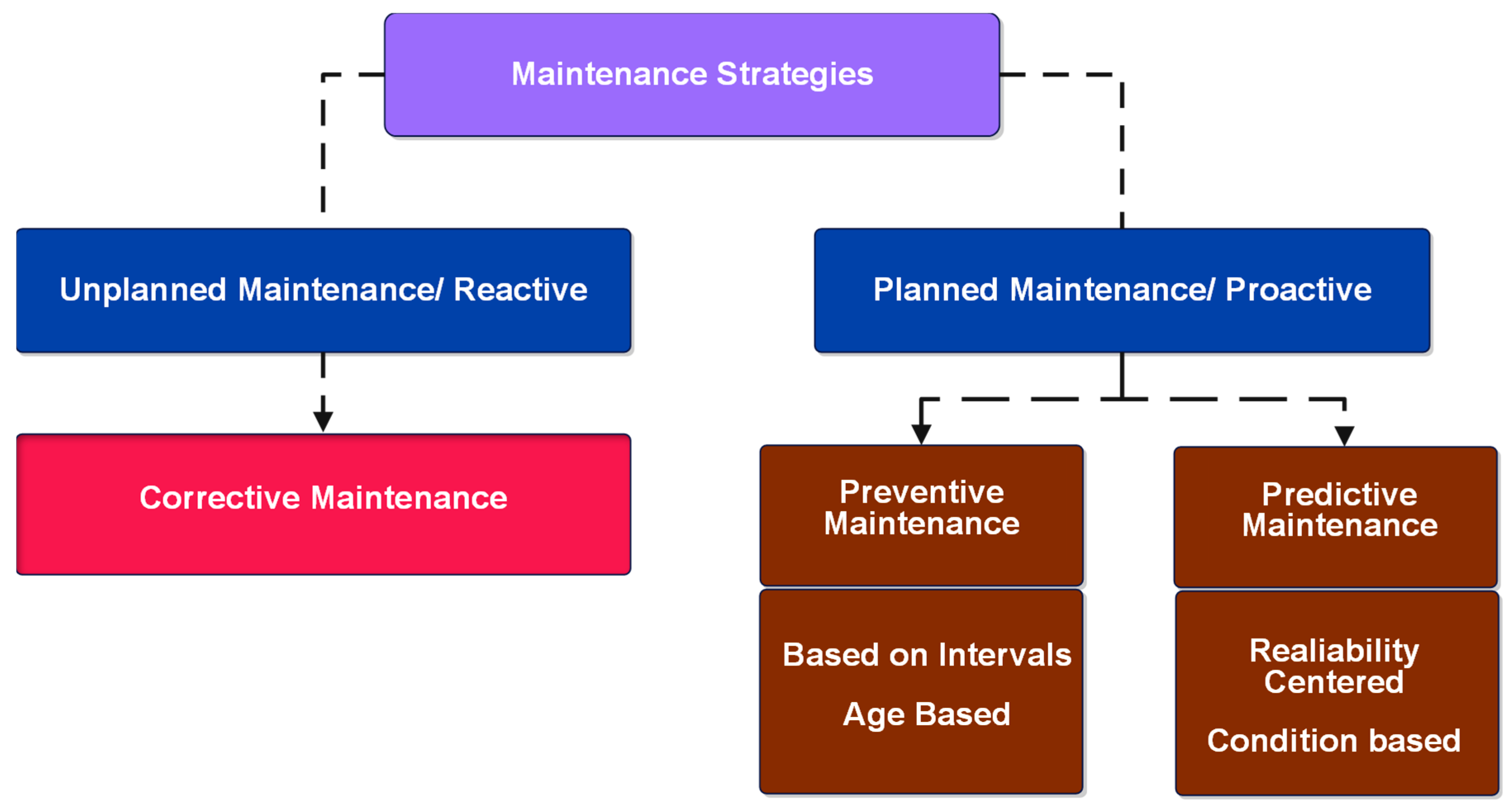
Figure 1. Hierarchy of maintenance strategies [6].
Processes 13 02707 g001
Figure 2. Solar wind energetic particles enter the Earth’s magnetic field lines [38].
Processes 13 02707 g002
Figure 3. Competitive Swarm Optimizer (CSO) process.
Processes 13 02707 g003
Figure 4. PLSCO flow chart.
Processes 13 02707 g004
Figure 5. Extreme Learning Machine.
Processes 13 02707 g005
Figure 6. ELM-PLSCO flow chart.
Processes 13 02707 g006
Figure 7. Convergence Curves of PLSCO and Compared Algorithms on CEC2015 30 dimension.
Processes 13 02707 g007aProcesses 13 02707 g007b
Figure 8. Convergence Curves of PLSCO and Compared Algorithms on CEC2020 30 dimension.
Processes 13 02707 g008aProcesses 13 02707 g008b
Figure 9. Box Plots of PLSCO and Compared Algorithms on CEC2015 30 dimension.
Processes 13 02707 g009aProcesses 13 02707 g009b
Figure 10. Box Plots of PLSCO and Compared Algorithms on CEC2020 30 dimension.
Processes 13 02707 g010aProcesses 13 02707 g010b
Figure 11. Diversity Plots of PLSCO and PLO.
Processes 13 02707 g011
Figure 12. Exploration vs. Exploitation.
Processes 13 02707 g012
Figure 13. Accuracy Plot of ELM-PLSCO and Compared Models.
Processes 13 02707 g013
Figure 14. Confusion Matrix of ELM-PLSCO and Compared Models.
Processes 13 02707 g014
Figure 15. ROC–AUC plots of ELM-PLSCO and Compared Models.
Processes 13 02707 g015
Figure 16. Feature Importance Score of ELM-PLSCO Model.
Processes 13 02707 g016
Table 1. Comparative Summary of the Proposed ELM-PLSCO Model and Prior ELM-Based Hybrid Optimization Models.
MethodCore Search PrincipleDynamic/Adaptive ControlDiversity/Perturbation MechanismELM Tuning Target
PSS-ELM [29] (Pareto-like Sequential Sampling ELM)Pareto-like Sequential Sampling using INFO and RUN strategies to select/update candidate solutions efficiently.Sequential optimizer cooperation for progressive refinement, balancing exploration and exploitation over iterations.Multi-strategy sampling patterns to maintain population diversity and stabilize convergence.Input weights (W) and biases (B)
HKF-ELM [30] (Heuristic Kalman Filter ELM)Kalman Filter–based state estimation applied to ELM parameter search.Noise-driven adaptive updates of state variables and gain coefficients.Dimensionality reduction in search space for faster, real-time parameter adaptation.Input weights (W) and biases (B)
JS-ELM [31] (Jellyfish Search ELM)Models’ jellyfish foraging and swarm drift in ocean currents.Time-control mechanism switching between passive drifting and active prey-chasing phases.Lévy-flight–like random walks to maintain diversity and reduce overfitting risk.Input weights (W) and biases (B)
WOA-ELM [32] (Whale Optimization Algorithm ELM)Bubble-net hunting strategy with spiral updating and encircling maneuvers.Adaptive adjustment of encircling radius and spiral pitch based on prey position.Hybrid spiral search and stochastic position updates to avoid premature convergence.Input weights (W) and biases (B)
IMOPSO-ELM [33] (Improved Multi-Objective Particle Swarm Optimization ELM)Multi-swarm cooperative PSO optimizing ELM input weights and hidden biases via RMSE, L2 norm, and L2,1 norm for network compactness and generalizationAdaptive multi-swarm and global-best selection strategies in IMOPSO; external elite archive guides particle updates to balance multiple objectives and prevent overfittingMaintains diversity via multi-objective dominance sorting and crowding distance.Input weights (W) and biases (B)
VMD–PLS–IASO–ELM [34] (Variational Mode Decomposition, Partial Least Squares, Improved Atom Search Optimization ELM)Combines VMD for signal decomposition, PLS extracts key features, and ASO with Simulated Annealing for parameter search.Annealing-based control of atomic interaction forces.Frequency-based decomposition from VMD plus stochastic perturbations in IASO to avoid local minima and maintain diversity in the search space.Input weights (W) and biases (B)
ELM-IFFA [35] (ELM with Improved Firefly Algorithm)Firefly Algorithm (FFA) enhanced with Lévy-flight-based random stepsDynamic light absorption coefficient and Lévy-flight step length adjust attraction range and exploration intensityLévy-flight-style randomization allows fireflies to jump out of local optima, maintaining diversity; random direction generation and population-based interactions prevent premature convergenceInput weights (W) and biases (B)
RF-IPWOA-ELM [36] (Random Forest, Improved Parallel Whale Optimization Algorithm ELM)Feature selection via RF, followed by parallelized WOA search.Two populations with different convergence factor strategies (nonlinear decrease tailored to random vs. chaotic initialization) adapt global/local search balanceRandom, chaotic sequence initialization ensures diverse starting points; immigration operator exchanges individuals by fitness tiers to maintain diversity and avoid local optimaInput weights (W) and biases (B)
ELM-GWO [37] (ELM with Grey Wolf Optimizer)Grey Wolf Optimizer’s leadership hierarchy (α, β, δ roles) guides search in the weight–bias spaceAdaptive role switching and encircling prey behavior; positions updated iteratively based on best wolvesRandom leader selection and position updates help escape local optimaInput weights (W) and biases (B)
ELM-PLSCO (Extreme Learning Machine, Polar Lights Salp Cooperative Optimizer)
(Current Work)
Cooperative hybrid of Polar Light Optimizer (PLO), Competitive Swarm Optimizer (CSO), and Salp Swarm Algorithm (SSA)Adaptive division of population into winners and losers through CSO; winners exploit via PLO, losers explore via SSA; global best dynamically updatedLeader–follower dynamics in SSA, competitive pairing in CSO, and stochastic updates maintain diversity and prevent premature convergenceInput weights (W) and biases (B)
Table 2. Parameter Settings.
AlgorithmParameter
ACGRIME μ = 4
AOµ = 0.00565, ω = 0.005 ,
α   =   δ = 0.1
AVOAL1 = 0.8, L2 = 0.2, w = 2.5, P1 = 0.6, P2 = 0.4, P3 = 0.6
OBLPFA α ,   β = [ 1 ,   2 ]
PFA α ,   β = [ 1 ,   2 ]
PO α = rand [0,1]/5, θ = rand [0,1] *   π
POA R = 0.2
SCA a = 2
PLO m = 100 , a = [ 1,1.5 ]
PLSCO m = 100 , a = [ 1,1.5 ] ,
  c 1   = [ 2 / e , 2 ]
Table 3. Results of PLSCO and other optimizers on CEC2015 30 dimensions.
ACGRIMEAOAVOAOBLPFAPFAPOPOASCAPLOPLSCO
F1AVG1.916 × 1054.862 × 10102.650 × 1082.687 × 1092.627 × 1094.689 × 10101.517 × 10101.354 × 10101.181 × 1077.105 × 104
STD1.217 × 1055.360 × 1092.422 × 1085.893 × 1085.530 × 1087.015 × 1097.118 × 1092.622 × 1093.604 × 1061.129 × 104
F2AVG1.622 × 1045.941 × 1045.167 × 1047.891 × 1041.030 × 1056.312 × 1042.631 × 1044.313 × 1047.850 × 1043.531 × 104
STD4.304 × 1032.703 × 1033.492 × 1032.941 × 1042.942 × 1046.476 × 1037.014 × 1036.064 × 1031.155 × 1041.050 × 104
F3AVG3.166 × 1023.427 × 1023.353 × 1023.311 × 1023.305 × 1023.398 × 1023.280 × 1023.367 × 1023.210 × 1023.157 × 102
STD2.8482.1653.5543.1662.7701.3512.8282.8482.2393.242
F4AVG4.359 × 1037.293 × 1035.298 × 1038.210 × 1038.173 × 1037.936 × 1034.057 × 1037.888 × 1034.672 × 1034.030 × 103
STD6.897 × 1026.898 × 1027.942 × 1023.651 × 1023.705 × 1023.048 × 1026.221 × 1022.939 × 1023.865 × 1027.001 × 102
F5AVG5.009 × 1025.026 × 1025.015 × 1025.034 × 1025.034 × 1025.029 × 1025.006 × 1025.029 × 1025.009 × 1025.006 × 102
STD3.245 × 10−14.607 × 10−15.769 × 10−14.159 × 10−13.287 × 10−13.902 × 10−12.188 × 10−13.195 × 10−11.994 × 10−13.812 × 10⁻¹
F6AVG6.004 × 1026.047 × 1026.005 × 1026.011 × 1026.010 × 1026.046 × 1026.023 × 1026.023 × 1026.007 × 1026.005 × 102
STD6.826 × 10−22.437 × 10−11.199 × 10−12.288 × 10−11.397 × 10−13.990 × 10−19.669 × 10−14.981 × 10−11.892 × 10−15.368 × 10⁻²
F7AVG7.005 × 1027.769 × 1027.005 × 1027.055 × 1027.059 × 1027.856 × 1027.315 × 1027.290 × 1027.005 × 1027.003 × 102
STD2.036 × 10−16.9342.180 × 10−12.5122.8241.182 × 1011.053 × 1014.5263.736 × 10−13.224 × 10⁻²
F8AVG8.099 × 10+25.126 × 1061.152 × 1033.417 × 1037.016 × 1035.097 × 1067.465 × 1049.573 × 1048.233 × 1028.093 × 102
STD4.1782.184 × 1063.410 × 1022.695 × 1031.213 × 1031.845 × 1065.296 × 1039.340 × 1043.1872.675
F9AVG9.124 × 10+29.136 × 1029.131 × 1029.135 × 1029.135 × 1029.135 × 1029.122 × 1029.134 × 1029.128 × 1029.124 × 102
STD3.941 × 10−11.297 × 10−12.712 × 10−11.903 × 10−12.249 × 10−11.490 × 10−14.731 × 10−11.934 × 10−14.352 × 10−13.075 × 10⁻¹
F10AVG5.396 × 1055.875 × 1076.376 × 1069.125 × 1069.551 × 1063.236 × 1075.819 × 1051.292 × 1079.916 × 1057.136 × 105
STD3.873 × 1051.799 × 1073.720 × 1066.068 × 1063.807 × 1061.164 × 1073.802 × 1055.507 × 1064.432 × 1054.413 × 105
F11AVG2.224 × 1031.841 × 1082.554 × 1044.359 × 1054.362 × 1051.374 × 1085.431 × 1031.029 × 1075.151 × 1031.204 × 103
STD2.032 × 1031.420 × 1081.930 × 1042.433 × 1052.906 × 1051.028 × 1084.836 × 1039.620 × 1064.718 × 1038.584 × 101
F12AVG2.719 × 1038.133 × 10129.235 × 10126.077 × 1051.538 × 1065.409 × 10112.869 × 1031.050 × 1093.197 × 1033.072 × 103
STD5.693 × 1021.153 × 10124.617 × 10124.340 × 1053.095 × 1053.022 × 10118.608 × 1026.374 × 1089.429 × 1024.269 × 102
F13AVG1.579 × 1032.411 × 1031.644 × 1031.711 × 1031.717 × 1031.798 × 1031.578 × 1031.590 × 1031.562 × 1031.559 × 103
STD2.798 × 1013.609 × 1023.002 × 1014.094 × 1014.464 × 1016.980 × 1011.085 × 1017.2281.3351.366 × 10−4
F14AVG2.001 × 1033.853 × 1034.993 × 1032.523 × 1032.521 × 1034.494 × 1032.413 × 1033.029 × 1032.133 × 1031.974 × 103
STD5.228 × 1011.020 × 1033.284 × 1033.156 × 1022.536 × 1027.527 × 1022.761 × 1022.259 × 1021.436 × 1021.111
F15AVG2.537 × 1032.968 × 1032.821 × 1032.983 × 1032.976 × 1032.998 × 1032.513 × 1032.920 × 1032.534 × 1032.441 × 103
STD1.450 × 1027.974 × 1017.609 × 1013.829 × 1013.358 × 1011.098 × 1023.521 × 1024.779 × 1018.323 × 1013.054 × 102
Table 4. Results of PLSCO and other Optimizers on CEC2020 30 dimensions.
ACGRIMEAOAVOAOBLPFAPFAPOPOASCAPLOPLSCO
F16AVG6.97 × 1034.55 × 10101.37 × 1094.56 × 1094.40 × 1094.70 × 10101.29 × 10101.70 × 10102.37 × 1073.95 × 104
STD6.92 × 1035.88 × 1099.51 × 1089.16 × 1089.67 × 1086.53 × 1095.19 × 1093.03 × 1098.34 × 1069.57 × 103
F17AVG1.56 × 1066.18 × 10121.15 × 10115.15 × 10114.42 × 10115.46 × 10121.71 × 10121.86 × 10122.69 × 1093.80 × 106
STD1.12 × 1066.97 × 10118.49 × 10109.43 × 10106.52 × 10107.29 × 10118.24 × 10112.33 × 10111.18 × 1098.82 × 105
F18AVG2.07 × 1051.86 × 10124.39 × 10101.59 × 10111.67 × 10111.74 × 10125.68 × 10116.06 × 10111.21 × 1091.74 × 106
STD7.86 × 1042.43 × 10113.86 × 10102.76 × 10103.91 × 10102.76 × 10112.27 × 10111.03 × 10114.36 × 1086.60 × 105
F19AVG1.91 × 1039.05 × 1052.48 × 1032.12 × 1032.06 × 1035.30 × 1059.44 × 1031.66 × 1041.92 × 1031.91 × 103
STD2.474.15 × 1057.47 × 1023.77 × 1021.46 × 1021.59 × 1058.59 × 1031.46 × 1041.872.71
F20AVG2.56 × 1052.28 × 1089.45 × 1059.33 × 1061.01 × 1075.30 × 1076.36 × 1051.18 × 1077.74 × 1052.16 × 105
STD1.15 × 1051.17 × 1088.39 × 1053.87 × 1064.96 × 1062.40 × 1074.00 × 1055.53 × 1063.76 × 1055.61 × 104
F21AVG3.31 × 1041.01 × 1083.29 × 1041.13 × 1061.02 × 1061.02 × 1083.59 × 1045.73 × 1061.05 × 1048.63 × 103
STD2.44 × 1047.95 × 1072.18 × 1045.93 × 1054.98 × 1056.50 × 1071.34 × 1044.37 × 1064.27 × 1036.23 × 103
F22AVG3.33 × 1059.96 × 1084.25 × 1061.95 × 1071.94 × 1073.08 × 1081.23 × 1063.49 × 1079.36 × 1052.61 × 105
STD2.44 × 1058.05 × 1082.49 × 1068.44 × 1067.65 × 1061.64 × 1087.76 × 1051.79 × 1076.72 × 1051.32 × 105
F23AVG2.39 × 1035.30 × 1032.55 × 1032.49 × 1032.49 × 1033.70 × 1032.85 × 1032.62 × 1032.38 × 1032.37 × 103
STD1.20 × 1019.48 × 1028.93 × 1012.48 × 1012.00 × 1013.59 × 1024.46 × 1024.89 × 1013.603.58
F24AVG2.63 × 1033.16 × 1046.02 × 1037.34 × 1037.43 × 1033.22 × 1041.73 × 1041.48 × 1043.00 × 1032.62 × 103
STD7.72 × 1011.30 × 1031.84 × 1037.28 × 1026.78 × 1023.00 × 1034.67 × 1031.27 × 1031.05 × 1024.26 × 101
F25AVG2.93 × 1035.80 × 1033.18 × 1033.21 × 1033.21 × 1036.25 × 1033.43 × 1033.62 × 1032.93 × 1032.93 × 103
STD9.565.56 × 1029.31 × 1019.67 × 1011.20 × 1026.85 × 1022.55 × 1021.49 × 1021.641.41 × 101
Table 5. Friedman and Wilcoxon Non-Parametric Analysis Results.
ACGRIMEAOAVOAOBLPFAPFAPOPOASCAPLOPLSCO
CEC2015Friedman Mean2.278.735.436.96.978.73.876.873.631.63
Friedman Rank21057894631
p-Value3.305 × 10−16.550 × 10−49.815 × 10−46.550 × 10−46.550 × 10−46.550 × 10−42.209 × 10−16.550 × 10−46.533 × 10−4-
CEC2020Friedman Mean1.959.64.55.75.59.46.37.82.81.45
Friedman Rank21046597831
p-Value8.886 × 10−15.062 × 10−35.062 × 10−35.062 × 10−35.062 × 10−35.062 × 10−35.062 × 10−35.062 × 10−37.632 × 10−3-
Table 6. Evaluation Metrics.
Evaluation MetricValue
Accuracy Score   Number   of   Correct   Predictions     Total   Predictions  
Recall Score   True   Positives     True   Positives + False   Negatives  
Specificity   True   Negatives     True   Negatives + False   Positives  
Precision   True   Positives     True   Positives + False   Positives  
F1-Score 2 ×   Precision   ×   Sensitivity     Precision   +   Sensitivity  
Table 7. Training Results of ELM-PLSCO and Compared Optimizers on Predictive Maintenance Predictions.
AccuracyRecallF1PrecisionSpecificityROC-AUC
ELM-ACGRIMEAVG0.944980.833800.825040.836420.966990.95842
STD3.4833 × 10−31.0473 × 10−21.1492 × 10−21.2322 × 10−22.0880 × 10−31.6508 × 10⁻²
Best0.955650.865800.858820.875710.973380.96830
ELM-AOAVG0.936730.809080.797530.810620.962040.93748
STD2.5019 × 10−37.4594 × 10−38.5143 × 10−38.7628 × 10−31.4983 × 10−31.5216 × 10⁻²
Best0.942040.825130.816670.829390.965220.95196
ELM-AVOAAVG0.937170.810430.798610.809850.962310.94697
STD5.9840 × 10−31.7981 × 10−22.1161 × 10−21.7712 × 10−23.5876 × 10−32.2907 × 10⁻²
Best0.950000.849210.843010.847260.970010.96569
ELM-OBLPFAAVG0.931570.793540.779970.793850.958950.93500
STD2.5022 × 10−37.5026 × 10-39.0911 × 10−37.9754 × 10−31.5003 × 10−31.9411 × 10⁻²
Best0.935440.805130.794310.805470.961270.95133
ELM-PFAAVG0.930400.790070.775970.790280.958250.93885
STD2.6446 × 10−37.9372 × 10−39.2766 × 10−38.2712 × 10−31.5870 × 10−31.8975 × 10⁻²
Best0.935810.806100.796580.811640.961490.95174
ELM-POAVG0.916740.749120.736870.755460.950040.93572
STD1.5943 × 10−24.7889 × 10−25.1919 × 10−24.4899 × 10−29.5756 × 10−32.3394 × 10⁻²
Best0.945990.836930.829480.840010.967590.95573
ELM-POAAVG0.938910.815640.804860.817540.963350.95430
STD4.2540 × 10−31.2755 × 10−21.4522 × 10−21.4342 × 10−22.5510 × 10−31.5111 × 10⁻²
Best0.946170.837540.830140.845540.967700.96257
ELM-SCAAVG0.931970.794770.781840.794440.959190.93724
STD2.6744 × 10−38.0207 × 10−39.5402 × 10−39.2014 × 10−31.6044 × 10−31.6640 × 10⁻²
Best0.937870.812830.802300.814260.962740.95226
ELM-PLOAVG0.937180.810340.799380.811290.962310.94835
STD2.5911 × 10−37.7804 × 10−38.8441 × 10−38.4426 × 10−31.5523 × 10-31.4603 × 10⁻²
Best0.943500.829270.820140.833940.966100.95984
ELM-PLSCOAVG0.956820.869510.864790.873660.974090.97265
STD3.2343 × 10−39.7067 × 10−31.0065 × 10−29.1041 × 10−31.9420 × 10−31.1501 × 10⁻²
Best0.962360.886090.880670.887680.977420.98163
ELMAVG0.927560.781490.764050.780790.956540.86978
STD1.1156 × 10−43.4839 × 10−44.2909 × 10−45.0514 × 10−46.7278 × 10−51.7422 × 10⁻⁴
Best0.927650.781770.764390.781220.956600.86990
Table 8. Test Results of ELM-PLSCO and Compared Optimizers on Predictive Maintenance Predictions.
AccuracyRecallF1PrecisionSpecificityROC-AUC
ELM-ACGRIMEAVG0.942960.831240.820360.830930.965780.95794
STD3.6422 × 10−31.0869 × 10−21.1953 × 10−21.2902 × 10−22.1895 × 10−31.7226 × 10⁻²
Best0.954130.864760.855260.871530.972500.96822
ELM-AOAVG0.934900.806940.793420.804730.960930.93654
STD2.5060 × 10−37.6073 × 10−38.4363 × 10−38.9505 × 10−31.5103 × 10−31.5305 × 10⁻²
Best0.940730.824210.813680.824530.964450.95125
ELM-AVOAAVG0.935300.808070.794490.804190.961170.94664
STD5.9249 × 10−31.7724 × 10−22.0922 × 10−21.8062 × 10−23.5619 × 10−32.3484 × 10⁻²
Best0.947950.845400.837860.841810.968760.96558
ELM-OBLPFAAVG0.929610.791230.775510.787470.957760.93336
STD2.6930 × 10−38.0910 × 10−39.9844 × 10−39.0900 × 10−31.6191 × 10−31.9308 × 10⁻²
Best0.934160.804900.792290.801720.960490.94989
ELM-PFAAVG0.928650.788230.772270.784670.957180.93737
STD2.7388 × 10−38.2006 × 10−39.7908 × 10−38.7281 × 10−31.6435 × 10−31.9135 × 10⁻²
Best0.934820.806860.796020.804570.960880.95128
ELM-POAVG0.915260.748070.733960.751560.949170.93512
STD1.5925 × 10−24.7671 × 10−25.1907 × 10−24.4197 × 10−29.5354 × 10−32.2797 × 10⁻²
Best0.944470.835530.826100.836050.966700.95500
ELM-POAAVG0.936770.812500.799700.810950.962060.95330
STD4.4501 × 10−31.3354 × 10−21.5188 × 10−21.5464 × 10−22.6744 × 10−31.5877 × 10⁻²
Best0.944110.834270.825400.840370.966450.96206
ELM-SCAAVG0.930040.792450.777530.788640.958020.93686
STD2.7910 × 10−38.3961 × 10−31.0006 × 10−29.6542 × 10−31.6760 × 10-31.7222 × 10⁻²
Best0.935050.806670.794940.809710.960990.95231
ELM-PLOAVG0.935550.809070.796110.806700.961330.94720
STD2.6505 × 10−37.9224 × 10−39.0507 × 10−38.6087 × 10−31.5953 × 10−31.4666 × 10⁻²
Best0.941730.827560.815510.827140.965030.95879
ELM-PLSCOAVG0.954650.865870.859360.867850.972800.97224
STD3.3773 × 10−31.0111 × 10−21.0633 × 10−29.6555 × 10−32.0226 × 10−31.2381 × 10⁻²
Best0.960030.882110.875070.881610.976010.98189
ELMAVG0.924870.777060.756770.770950.954900.86649
STD1.4291 × 10−44.0735 × 10−44.8355 × 10−44.9587 × 10−48.4736 × 10−59.0289 × 10⁻⁵
Best0.924990.777390.757160.771350.954970.86656
Table 9. Computation Time Comparison of ELM-PLSCO and other Models.
ELM-ACGRIMEELM-AOELM-AVOAELM-OBLPFAELM-PFAELM-POELM-POAELM-SCAELM-PLSCOELM-PLOELM
376.51389.58135.21245.58137.141454.18446.77132.45287.21132.103.37
Disclaimer/Publisher’s Note: The statements, opinions and data contained in all publications are solely those of the individual author(s) and contributor(s) and not of MDPI and/or the editor(s). MDPI and/or the editor(s) disclaim responsibility for any injury to people or property resulting from any ideas, methods, instructions or products referred to in the content.