Article

Ultra-Short-Term Wind Power Prediction with Multi-Scale Feature Extraction Under IVMD

1
Hubei Provincial Engineering Research Center of Intelligent Energy Technology, Yichang 443002, China
2
College of Electrical and New Energy, China Three Gorges University, Yichang 443002, China
*
Author to whom correspondence should be addressed.
Processes 2025, 13(8), 2606; https://doi.org/10.3390/pr13082606
Submission received: 17 July 2025 / Revised: 9 August 2025 / Accepted: 15 August 2025 / Published: 18 August 2025
(This article belongs to the Section Energy Systems)

Abstract

To mitigate wind power intermittency effects on forecasting accuracy, this study proposes a novel ultra-short-term prediction method based on improved variational mode decomposition (IVMD) and multi-scale feature extraction. First, the maximum information coefficient identified meteorological features strongly correlated with wind power, such as wind speed and wind direction, thereby reducing model input dimensionality. Permutation entropy then served as the fitness function for the sparrow search algorithm (SSA), enabling adaptive IVMD parameter optimization for effective decomposition of non-stationary sequences. The resulting intrinsic mode functions and key meteorological features were input into a prediction model integrating a temporal convolutional network (TCN) and bidirectional gated recurrent unit (BiGRU) to capture global trends and local fluctuations. The SSA was reapplied to optimize TCN-BiGRU hyperparameters, enhancing adaptability. Simulations using operational data from a Xinjiang wind farm demonstrated that the proposed method achieved a coefficient of determination (R2) of 0.996, representing an absolute increase of 0.060 over the XGBoost benchmark (R2 = 0.936). This confirms significant enhancement of ultra-short-term forecasting accuracy.

1. Introduction

1.1. Motivation

The transition of the power system’s energy structure from fossil fuels to renewable sources represents a foundational imperative and strategic necessity for achieving China’s “dual carbon goals” [1]. However, the inherent intermittency and variability of wind power output, driven by meteorological factors, pose substantial challenges to power grid security and operational stability [2,3], manifested as follows: (1) Increased reserve capacity requirements (e.g., up to 20–30% of installed wind capacity to compensate for forecast errors); (2) Frequency deviation risks exceeding ±0.5 Hz under prediction inaccuracies > 15%; consequently, high-accuracy ultra-short-term wind power forecasting (≤4-h horizon) serves as a critical technological solution for facilitating large-scale wind integration. This capability is indispensable for optimizing grid dispatch operations and ensuring effective power system frequency regulation [4,5].

1.2. Literature Review

Scholars domestically and internationally have devoted themselves to researching wind power prediction methods, which primarily fall into two categories: physical modeling and statistical analysis [6]. Physical prediction models, constructed based on wind turbines, wind farm geomorphological features, and meteorological information [7,8], often yield biased predictions due to errors in input data. Additionally, the complexity of physical modeling processes results in limited generalizability. Although statistical methods—such as support vector machines [9], extreme learning machines [10], and artificial neural networks [11]—are simpler than physical modeling, their limitation lies in insufficient extraction of deeper data features when handling complex nonlinear problems.
Data-driven deep learning, as a statistical analysis approach, has been widely adopted in wind power prediction due to its strong feature extraction and nonlinear fitting capabilities [12,13]. Shallow deep learning models include convolutional neural networks (CNNs) [14] and recurrent neural networks (RNNs) [15]. CNNs exhibit significant nonlinear feature extraction capabilities. Reference [16] demonstrated the application of CNNs to wind speed prediction, achieving a 6.9% improvement in prediction accuracy based on the Dutch test set. To mitigate the vanishing gradient problem encountered by RNNs during long sequence processing, the gated recurrent unit (GRU), a simplified model variant, was proposed. However, shallow models often struggle to achieve the necessary prediction accuracy. Consequently, research has increasingly focused on leveraging ensemble models to enhance performance. Reference [17] employed a model architecture integrating CNN, bidirectional gated recurrent unit (BiGRU), and attention mechanisms. Through refinement of the prediction model’s loss function and compensation for prediction biases in low wind speed segments, wind power prediction accuracy was enhanced. This method achieved a 14.4% reduction in prediction error relative to a standalone CNN architecture. Although effective, this approach neglects the high computational burden caused by high-dimensional input sequences. Consequently, reference [18] employed Pearson correlation coefficients to screen key meteorological factors, reducing model input dimensionality and computational requirements. Improved prediction results were subsequently achieved using CNN and enhanced long short-term memory networks (LSTMs). However, the accuracy of such hybrid models remains constrained by inadequate hyperparameter tuning [19]. To optimize model hyperparameters, population-based metaheuristic algorithms can be employed, such as particle swarm optimization (PSO) [20] and whale optimization algorithm (WOA) [21]. Leveraging their global convergence properties, these intelligent optimization methods facilitate automated hyperparameter tuning for predictive models. Reference [22] proposed a hybrid architecture integrating frequency attention mechanisms with a temporal convolutional network (TCN). The authors noted that TCN incorporates the fundamental principles of one-dimensional CNN while introducing structural enhancements specifically designed for processing temporal data. In their framework, PSO was employed to determine optimal hyperparameters, including TCN kernel dimensions and residual block counts. Simulation experiments subsequently validated PSO’s effectiveness for model parameter optimization. Nevertheless, existing methods exhibit adaptive limitations in capturing time-varying statistical characteristics when processing non-stationary wind power time series.
Currently, decomposition methods that address wind power non-stationarity by decomposing raw sequences into multiple intrinsic mode functions with distinct bandwidths have gained significant attention [23,24,25]. Reference [23] applied empirical mode decomposition (EMD) to preprocess raw wind power data, but this method is prone to mode mixing during noise reduction. Reference [24] employed a multi-channel noise superposition strategy based on ensemble empirical mode decomposition (EEMD) to mitigate the modal aliasing problem inherent in EMD. However, residual white noise (where high-frequency noise sensitivity reached 0.21) still induced distortion in the high-frequency signal components. This distortion constrained the input quality for subsequent predictive models. Reference [25] introduced variational mode decomposition (VMD), feeding the decomposed modes into a Bayesian-optimized gated recurrent unit for prediction. While VMD circumvents EEMD’s noise-induced limitations and achieves favorable results, its decomposition quality is constrained by parameter selection. Critically, the traditional parameter determination method based on center-frequency observation exhibits strong subjectivity. Population-based metaheuristic algorithms offer potential performance improvements. However, Bayesian inference methods present limitations for parameter optimization scenarios. Due to their inherent dependence on prior probability distributions, Bayesian approaches may inadequately capture complex empirical data distributions, often resulting in convergence to local optima.

1.3. Main Contributions

Building upon existing research, this study proposes a novel forecasting framework integrating an adaptive decomposition method with a hybrid feature extraction model to further enhance wind power prediction accuracy. Specifically, we introduce an ultra-short-term forecasting method based on improved variational mode decomposition (IVMD) and multi-scale feature extraction. Firstly, the maximum information coefficient (MIC) is employed to screen meteorological features exhibiting strong correlations with wind power data, mitigating feature redundancy. Subsequently, utilizing permutation entropy as the fitness criterion, the sparrow search algorithm (SSA) dynamically identifies the optimal number of modes and penalty factor for VMD, enabling adaptive decoupling of the original wind power sequence’s intrinsic mode functions (IMFs). These decomposed IMFs are then integrated with key meteorological features to form the input for the prediction model. Finally, SSA optimizes the hyperparameters of the TCN-BiGRU multi-scale feature extraction network, constructing a prediction model that synergistically combines global trend response with local feature focus. The methodology comprises three key stages:
(1)
MIC-driven feature selection identifying key meteorological predictors.
(2)
Entropy-guided adaptive VMD via SSA-tuned decomposition parameters.
(3)
Multiscale hybrid forecasting integrating mode-feature fusion and SSA-optimized TCN-BiGRU architecture.
The efficacy of the proposed method is rigorously validated through comprehensive ablation studies and comparative simulation experiments.

1.4. Paper Organization

The remainder of this paper is structured as follows: Section 2 delineates the overall framework of the proposed methodology. Section 3 elaborates on wind power signal processing via the IVMD. Section 4 details the architecture of the multiscale feature extraction model. Section 5 validates the approach through comparative experiments. Section 6 concludes with critical implications and research findings.

2. Overall Construction Based on IVMD and Multi-Scale Feature Extraction Model

To mitigate grid stability challenges induced by high-amplitude power fluctuations in wind farms and enhance ultra-short-term forecasting accuracy, this study proposes a novel prediction framework integrating IVMD with SSA-TCN-BiGRU. The architectural schematic is illustrated in Figure 1.
The steps for establishing the process architecture are as follows:
  • MIC feature dimension reduction. The original data contains some meteorological features with weak correlation with wind power; eliminating redundant meteorological features can not only reduce the input dimension of the model, but also improve the model’s generalization ability [26].
    Compared to traditional methods like Pearson’s correlation analysis, MIC can evaluate correlations for both linear and nonlinear relationships, offering broad universality and equitability. The MIC calculation formula is as follows:
    I ( x , y ) = P ( x , y ) log 2 ( P ( x , y ) P ( x ) P ( y ) ) d x d y MIC ( x , y ) = max a b < λ I ( x , y ) log 2 min ( a , b )
    where I ( x , y ) denotes the mutual information between variables x and y ; P ( x , y ) represents the joint probability distribution of x and y ; P ( x ) and P ( y ) are the marginal probability distributions of x and y , respectively; a and b are the number of cells for each axis in performing the scatter-grid distribution, respectively; and λ is approximately 0.6 times the sample size.
  • The raw wind power sequences were subjected to signal decomposition and denoising preprocessing. To address the randomness of wind power, the IVMD method was employed to adaptively decompose and denoise the original wind power signal, yielding a set of K relatively smooth components, denoted as { I M F 1 , I M F 2 , , I M F K } .
  • Data preprocessing and division. To mitigate the influence of differing dimensions on prediction results, each component is first individually integrated with key meteorological features before undergoing uniform normalization, as defined in Equation (2). The processed datasets were then partitioned into training and testing subsets.
    x = x x min x max x min
    where x and x are the data before and after normalization, respectively; x max and x min are the maximum and minimum values of the data columns, respectively.
  • Prediction model construction. The training set data are input into the TCN-BiGRU framework for model training, while the optimal parameter combinations are obtained by iterative tuning using SSA, and the optimized model is applied to the test set data, after which the prediction results of each component are output.
  • Error evaluation analysis. The wind power prediction value is obtained by superimposing the inverse normalization of each component, and the prediction results are analyzed according to the error evaluation indexes and comparison models to quantitatively determine the performance of the model. To impartially assess model efficacy, three established metrics are employed: root mean square error (RMSE), mean absolute error (MAE), and coefficient of determination R 2 . These quantify forecasting precision through the following formulations:
    e RMSE = 1 S i = 1 S ( y i y ^ i ) 2
    e MAE = 1 S i = 1 S | y i y ^ i |
    R 2 = 1 i = 1 S ( y ^ i y i ) 2 i = 1 S ( y ¯ y i ) 2
    where S denotes the total sample count; y i and y ^ i represent the actual and forecasted values for the i-th sample, respectively; and y ¯ indicates the mean of y i .
Smaller values of e RMSE and e MAE indicate smaller model prediction errors and higher accuracy, and the closer R 2 is to 1, the better the model fits the data.

3. Wind Power Data Decomposition Based on IVMD

The traditional VMD signal processing method has obvious parameter configuration constraints, relying solely on the center frequency observation method to determine the number of modes K , which not only suffers from the defect of high operational subjectivity, but also fails to synergistically consider the critical impact of the penalty factor σ on the bandwidth constraints during the signal decomposition process, which may lead to insufficient K for decomposition, thus ignoring the key features of the signal, and excessive K will bring redundant noises; a larger σ will make the bandwidth of each IMF too narrow and lose certain signal details, while smaller σ leads to larger IMF bandwidth and sometimes oscillations [27]. Adaptive decoupling of signals can be achieved by optimizing the K and σ of the VMD through SSA.

3.1. Processing of Non-Stationary Wind Power Signals

Wind power generation exhibits inherent non-stationarity primarily due to its dependence on multiple, fluctuating meteorological factors. To address this, the VMD algorithm offers an effective approach. The VMD method operates in a complete and non-recursive manner, decomposing non-stationary wind power sequences into a finite number of intrinsic mode functions (IMFs). Each IMF exhibits distinct center frequencies and limited bandwidth [28,29]. Fundamentally, VMD constitutes a constrained variational optimization problem, formally expressed as follows:
min { u k } , { ω k } k = 1 K t δ ( t ) + j π t u k ( t ) e j ω k t 2 2 s . t . k = 1 K u k ( t ) = s ( t )
where s ( t ) represents the original wind power time-series signal; u k is each eigenmode component; ω k corresponds to the center frequency of each IMF; K corresponds to the center frequency of each IMF; t denotes the partial derivative with respect to time t ; δ ( t ) represents the Dirac delta function,; * denotes the convolution operation; and 2 2 signifies the squared L 2 -norm.
The introduction of a quadratic penalty factor σ and Lagrange multiplier λ facilitates computational tractability, thereby reformulating the constrained optimization framework as an unconstrained problem:
L ( t ) = σ k = 1 K t { δ ( t ) + j π t u k ( t ) e j ω k t } 2 2 + s ( t ) k = 1 K u k ( t ) 2 2 + λ ( t ) , s ( t ) k = 1 K u k ( t )
where the augmented Lagrangian functional L ( t ) is defined, with , representing the inner product operator for correlation functions.
Each IMF component and its center frequency are updated by alternating iterations as follows:
u ^ k m + 1 ( ω ) = s ^ ( ω ) i = 1 , i < k K u ^ i m + 1 ( ω ) i = 1 , i > k K u ^ i m ( ω ) + λ ^ m ( ω ) / 2 1 + 2 σ ( ω ω k m ) 2
ω k m + 1 = 0 + ω u ^ k m + 1 ( ω ) 2 d ω 0 + u ^ k m + 1 ( ω ) 2 d ω
where u ^ k m + 1 ( ω ) , s ^ ( ω ) , λ ^ m ( ω ) and u ^ i m ( ω ) are the fourier transforms of u k m + 1 ( t ) , s ( t ) , λ m ( t ) and u i m ( t ) , respectively; m is the number of iterations.

3.2. Principle Explanation of IVMD

The SSA is employed to optimize critical parameters within the VMD framework. The SSA, classified within the group intelligence optimization algorithms, simulates sparrow foraging and anti-predation behaviors. Within the population, sparrows are categorized into two functional roles: explorers and followers [30]. Each sparrow is randomly assigned an initial X i of the i-th sparrow, denoted as [ K i , σ i ] , that corresponds to a unique solution to the fitness function f i . The update of sparrows’ foraging positions throughout the optimization process directly maps to the iterative refinement of solutions in search of the global optimum.
Explorers are the better-adapted individuals in the sparrow population and are responsible for searching for food sources. The process of updating the position of explorers is as follows:
X i , j n + 1 = X i , j n exp ( i t iter max )         R 2 < S T X i , j n + Q E             R 2 S T
where n is the current iteration index; X i , j n represents the spatial coordinate of the i th sparrow in the j th dimension; t denotes a uniformly distributed random variable on (0, 1]; iter max is the maximum iteration threshold; Q is the perturbation factor that follows the standard normal distribution; E is the matrix whose elements are all 1; and R 2 and S T are the environmental risk coefficient and the safety threshold, respectively.
A follower h will compete for the explorer’s food if he finds that the fitness value of explorer i at another location satisfies f ( X h n + 1 ) > f ( X i n ) , i.e., the current optimal solution occurs. The iterative formula for the position of a follower is as follows:
X i , j n + 1 = Q exp ( X w n X i , j n i 2 )               i > m / 2 X P n + 1 + X i , j n X P n + 1 A + E               i m / 2
where m quantifies the sparrow population size; X w n represents the worst-positioned individual in the current population; X p denotes the optimal position occupied by followers; A + is A T ( A A T ) 1 and the elements of the matrix are 1 or −1.
A total of 10% to 20% of the sparrows in the population will be randomly assigned to act as vigilantes, who are responsible for signaling when danger is detected, and then the individuals will quickly move to a safe area for foraging, to avoid local optimal solutions of the fitness function, which is expressed as follows:
X i , j n + 1 = X b n + β X i , j n X b n           f i > f b X i , j n + k ( X i , j n X w n f i f w + γ )           f i = f b
where X b is the current optimal position of the sparrow; f i represents the fitness value of the i-th individual; β follows a standard normal distribution; f b and f w are the current global optimal and worst fitness values, respectively; k is a random number of [−1, 1]; and γ is the value of the minimal constant.
Before optimizing the VMD parameters, it is necessary to construct a fitness function. Permutation entropy, as a nonlinear dynamic feature, characterizes the complexity of time series through phase space reconstruction [31]. The permutation entropy calculation process is as follows:
  • Perform phase space reconstruction for a given time series { u ( i ) , i = 1 , 2 , , S } and denote each reconstructed component U ( j ) as follows:
    U ( j ) = [ u ( j ) , u ( j + τ ) , , u ( j + ( m 1 ) τ ) ]
    where m denotes the embedding dimensionality; τ indicates the count of delay times; and the number of reconstruction components is j = S ( m 1 ) τ .
  • The elements in each reconstructed component U ( j ) after sorting in ascending numerical order:
    U ( j ) = [ u ( j + ( j 1 1 ) τ ) u ( j + ( j 2 1 ) τ ) u ( j + ( j m 1 ) τ ) ]
    where j 1 , j 2 , , j m is the column number of the reconstructed component before sorting. Therefore, the m-dimensional U ( j ) component can be mapped to different ( j 1 , j 2 , , j m ) , with a total of m ! sorting modes.
  • Denote by P 1 , P 2 , , P N the probability of occurrence of N different sorting patterns and satisfy m ! N . The entropy of the arrangement of the time series { u ( i ) , i = 1 , 2 , , S } can be expressed as follows:
    H PE ( m ) = j = 1 N P j ln P j
Permutation entropy quantifies sequence complexity based on phase space reconstruction: decreasing entropy values indicate stronger sequence periodicity and regularity, while increasing values signify greater multiscale fluctuations or noise content. Under adequate VMD, each IMF should predominantly reflect distinct scales of stationary components within the original sequence. Consequently, the permutation entropy of each individual IMF is expected to be minimized, while their entropy values should simultaneously exhibit significant differentiation.

3.3. Overall Construction of IVMD

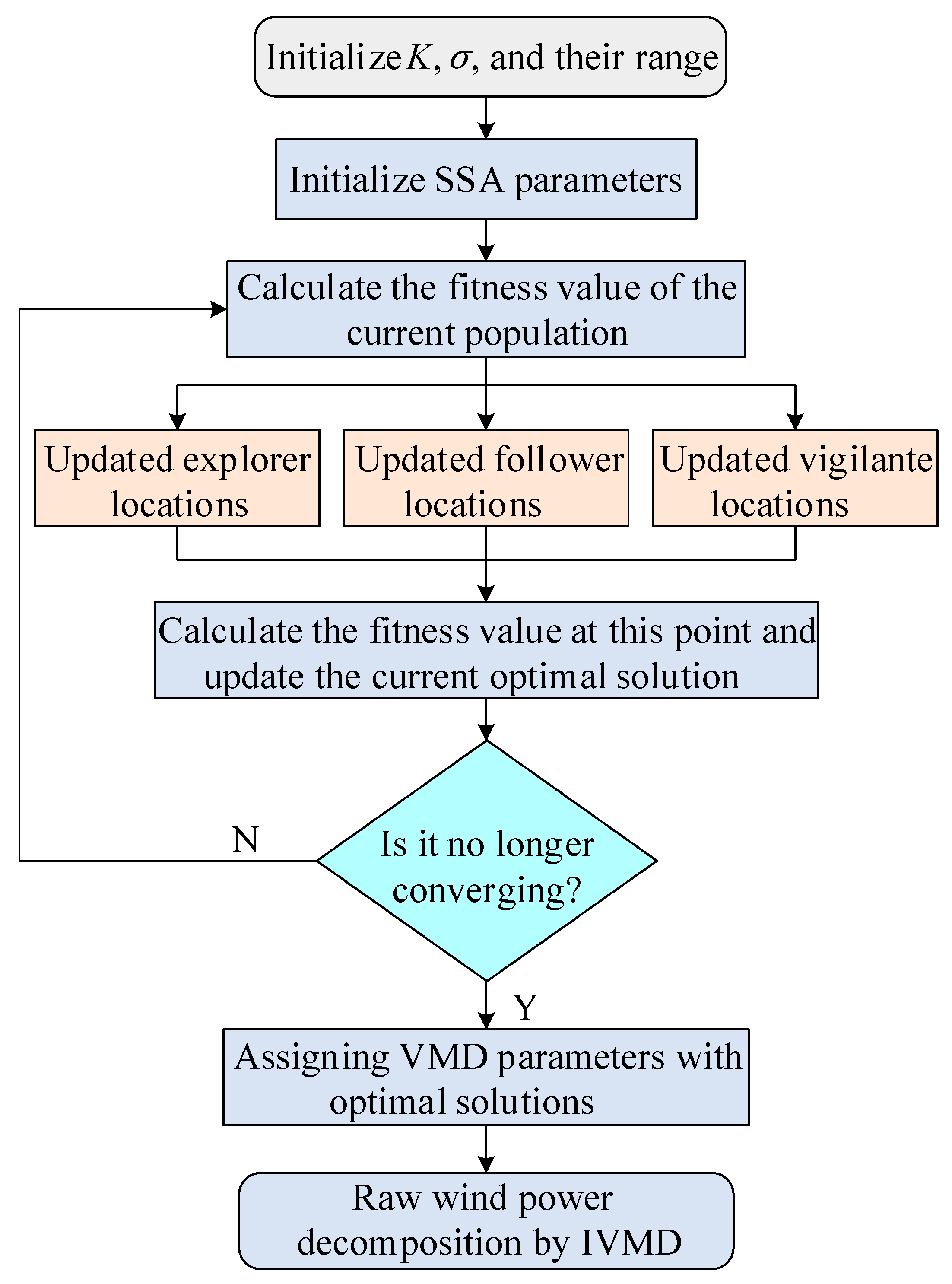
The parameter adaptation framework of the VMD parameter optimization method based on the permutation entropy measure is constructed by fusing SSA so as to realize the adaptive decomposition of non-stationary wind power data. The IVMD flowchart is shown in Figure 2.
The specific steps for establishing IVMD are as follows:
  • Initialize the K and σ parameters to find the optimal range, set the number of sparrow populations with the maximum number of iterations, and use permutation entropy as the fitness function.
  • For each sparrow’s current position X i = [ K i , σ i ] , use VMD to decompose in terms of K i and σ i to obtain K i IMFs, calculate the permutation entropy value of each IMF component, and record the value of the minimum and maximum fitness at this point and its corresponding parameter combination method.
  • Upon completion of a single iteration, the fitness values of all parameter combinations are reassessed. The positional information of explorers, followers, and vigilantes is dynamically updated, while the current global optimal and suboptimal fitness values—along with their corresponding parameter combinations—are synchronously propagated across the system.
  • When the preset maximum number of iterations or the convergence threshold of the fitness function is reached, the optimal parameter combination is output; otherwise, return to step 2 to continue the iterative calculation.
  • Perform VMD modal decomposition of the raw wind power signal using the optimized parameter configuration.

4. Design of Multiscale Feature Extraction Prediction Models

4.1. Temporal Convolutional Neural Networks

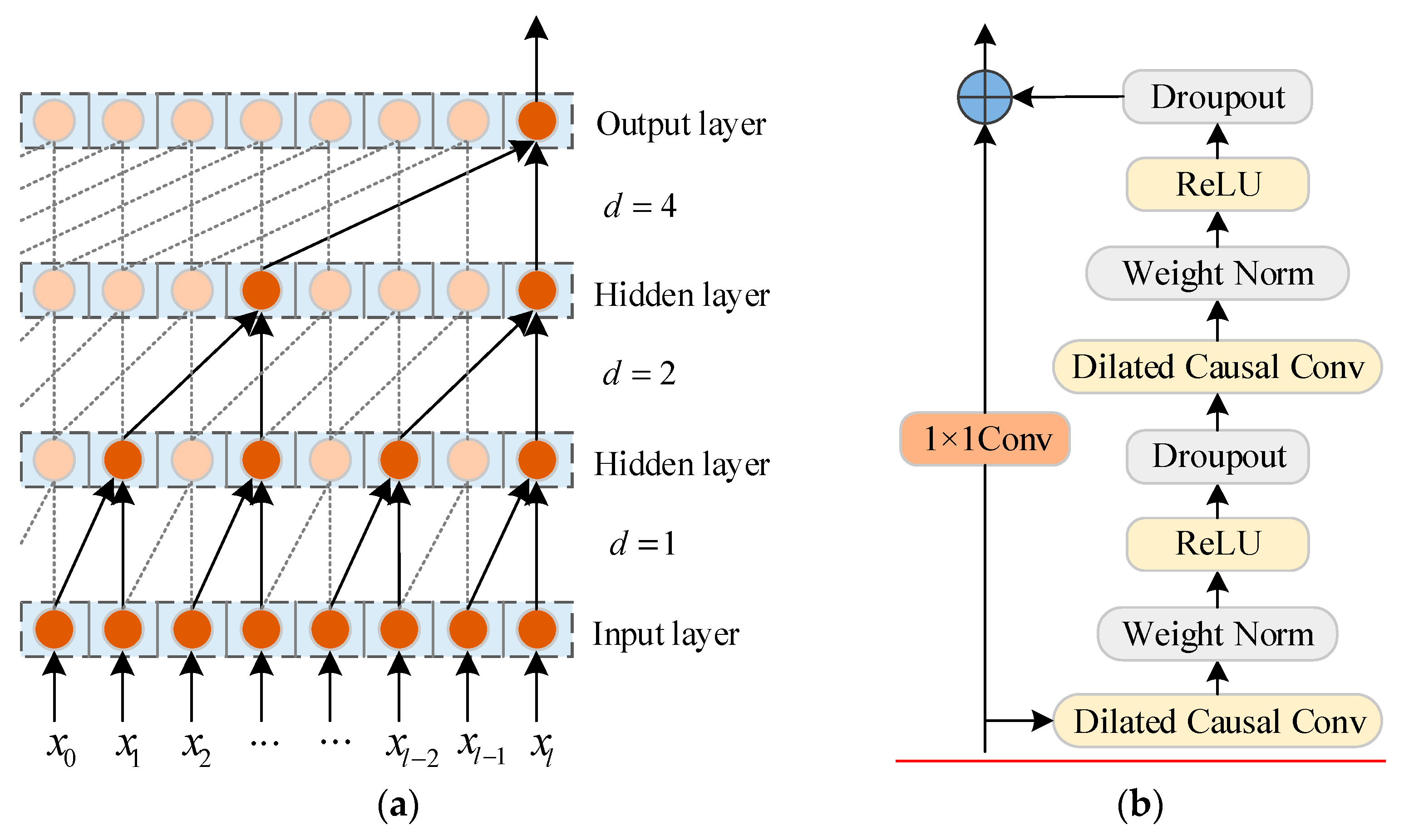
TCN is composed of dilated causal convolutions and a residual block stacking mechanism, which has better parallel processing capability and a flexible extended sensing range, so as to enhance the extraction capability of long time-series global trend features [32]. Its structure is shown in Figure 3.
Dilated causal convolutions extend the sensing field through the cascade-increasing dilation coefficients d, so that the shallow network can also capture long-distance dependency relationships across the time-steps, and thus avoid the traditional convolutional network due to the sequence of cascade-by-cascade transmission of the problem of information decay. Its structure is shown in Figure 3a.
For a convolution kernel f defined on a set { 0 , 1 , , k 1 } , the dilation causal convolution F acting on an element of the sequence at position s is defined as follows:
F ( s ) = ( X f ) ( s ) = i = 0 k 1 f ( i ) X s i d
where X is a one-dimensional input sequence; f ( i ) is the value of the i th element in the convolution kernel; X s i d represents the direction of the historical data used in the convolution operation; and k is the size of the convolution kernel.
The unit residual block contains a pair of dilated causal convolutions and the normalization and activation modules accompanying them, and its structure is shown in Figure 3b. The problem of vanishing or exploding gradients under deep networks is effectively avoided by stacking multiple layers of residual blocks while maintaining stable network performance.

4.2. Bidirectional Gated Recurrent Units

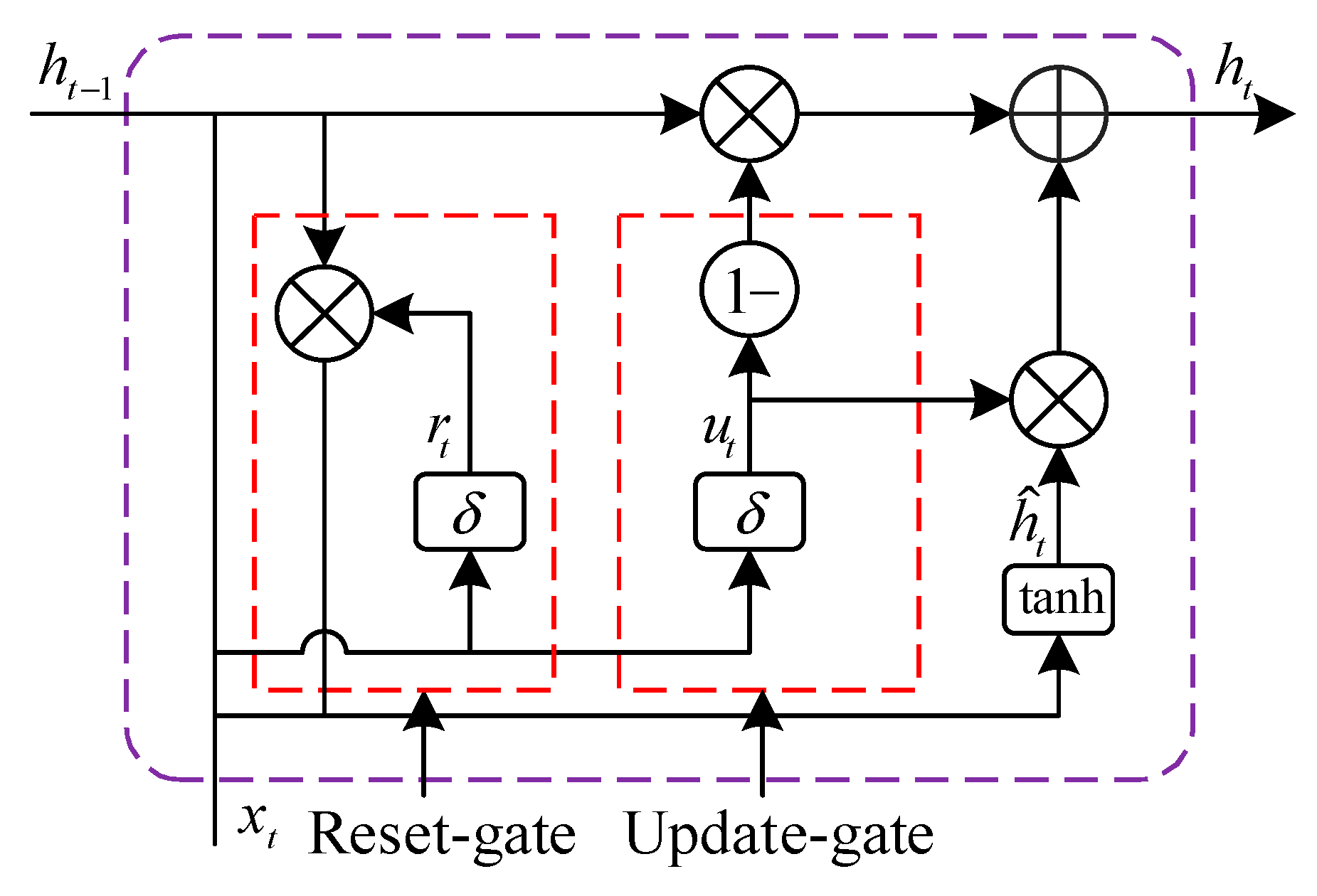
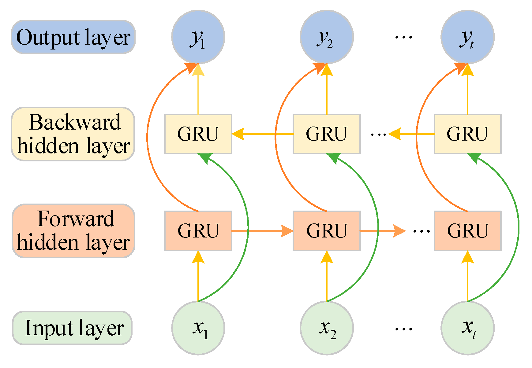
BiGRU is a structural variant of gated recurrent unit (GRU), which consists of two layers of GRUs with the same but opposite directions of transferring information, allowing the model to synchronize the fusion of past and future feature factors at each time node [33]; the gating mechanism of the GRU achieves precise focusing on local features within the time window through the dynamic weight allocation of the update gate and the reset gate. The structure of GRU is shown in Figure 4.
Let x t and h t be the inputs and outputs of the GRU model at time t , respectively, and the remaining GRU network parameters are expressed as follows:
r t = δ ( W r [ h t 1 , x t ] ) u t = δ ( W u [ h t 1 , x t ] ) h ^ t = tanh ( W [ r t h t 1 , x t ] ) h t = ( 1 u t ) h t 1 + u t h ^ t
where h ^ t denotes the candidate hidden-state; W r , W u , and W correspond to the weight matrices of the reset-gate, update-gate, and candidate-hidden-state, respectively; δ and tanh are the sigmoid and hyperbolic tangent activation functions, respectively; and r t and u t are the reset gate and update gate, respectively.
According to the structural characteristics of GRU, its reset gate filters redundant memories irrelevant to the current by different δ to avoid their dilution effect on the local abrupt change characterization information. The update gate will adaptively enhance the interaction strength of neighboring temporal signals within the local window, thus improving the characterization strength of the instantaneous abrupt change information.
The structure of the BiGRU network is shown in Figure 5, x t and y t are inputs and outputs at time t , respectively; the forward hidden layer extracts historical-to-current trend features along the time series forward, and the backward hidden layer captures potential correlation information from the future to the present, and the two synergistically further enhance the feature information capturing ability.

4.3. Hyperparameter Optimization of Multiscale Feature Extraction Models

Due to its inherent structural architecture, the TCN-BiGRU multiscale feature extraction framework facilitates comprehensive capture of both global evolutionary trends and local fluctuation patterns within wind power data. Regarding the potential degradation in model fitting efficacy and generalization capability resulting from subjective hyperparameter selection in TCN-BiGRU, SSA is employed to optimize these hyperparameters. The corresponding optimization procedure is illustrated in Figure 6.
For the role of model hyperparameters, five generalized ones are selected for optimization, which contain learning rate, regularization coefficient, number of BiGRU neurons, TCN convolutional kernel size, and its number. In addition, the model optimizer selects Adam, and the number of training iterations is set to 50. The SSA optimization process is similar to that of Section 3.3, which is a multi-objective parameter optimization process; the difference is that the sparrow position information represents the above generalized hyperparameters, and the fitness function adopts the mean-square error (MSE). In each training epoch, the model calculates the MSE metric. After completing 50 epochs, the model selects the initial parameter combination corresponding to the minimum MSE as the optimal network parameters.

5. Simulation Analysis

5.1. Data Preparation and Correlation Analysis

Experimental data were acquired from wind farms in Xinjiang, China, spanning the period from 1 January to 1 March, 2019. The dataset comprises 5500 samples collected at 15-min intervals. To evaluate the predictive performance of the model, the samples were partitioned into training and test sets at a 9:1 ratio, respectively. The modeling framework utilizes historical wind power outputs and critical meteorological parameters from the preceding two hours to forecast wind power generation for the subsequent 15-min interval.
The prediction model was implemented within the PyTorch 1.12.0 deep learning framework under a Python 3.9 integrated development environment. Experimental computations were executed on a Windows 11 operating system, utilizing an NVIDIA GeForce RTX 2070 SUPER GPU (14,000 MHz) with 16 GB RAM. NVIDIA is headquartered in Santa Clara, CA, USA. For the problem of fluctuating prediction results caused by random initialization of weakly correlated parameters of neural networks, the average of the results of six independent repetitions of the experiment is used as the final output.
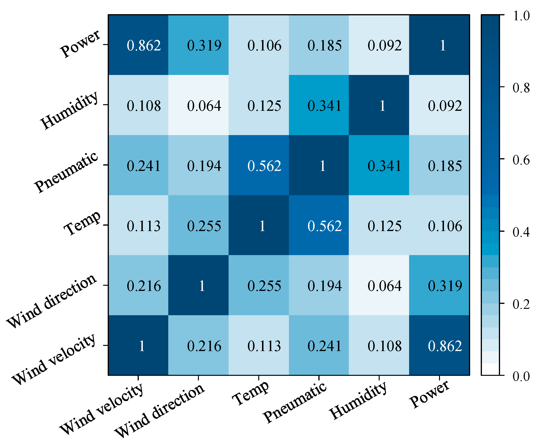
In order to reduce the training burden of the prediction model, the meteorological features that are strongly correlated with wind power are filtered using MIC, and the MIC correlation heat map of each meteorological factor is shown in Figure 7.
As indicated by the correlation analysis in Figure 7, wind speed and direction exhibiting a maximal information coefficient MIC 0.3 relative to wind power generation were identified as input variables for the forecasting model [34].

5.2. Model Parameter Settings

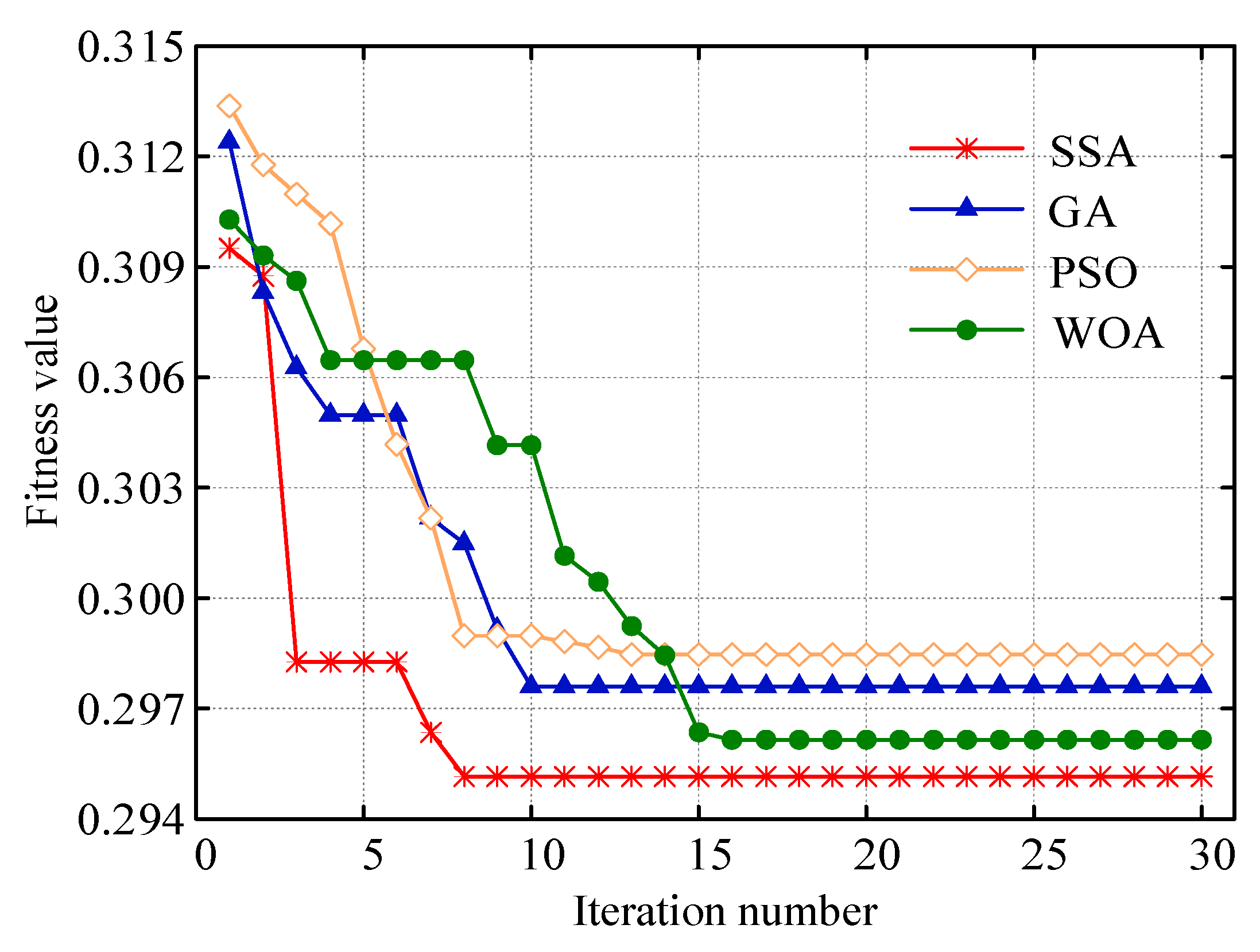
The validity and convergence of the SSA algorithm should be verified before optimizing the parameters of the model concerned, and SSA is compared with common particle swarm optimization (PSO), genetic algorithm (GA), and whale optimization algorithm (WOA) are compared in the experiment. The experimental configuration employed a safety threshold ( S T = 0.8 ) and risk coefficient ( R 2 = 0.2 ) for the SSA. All four benchmark algorithms utilized identical parameterization: population size N = 20 and maximum iterations T = 30 . Figure 8 demonstrates the adaptive convergence characteristics under this configuration.
As demonstrated in Figure 8, the SSA attains its minimum fitness value within eight iterations, outperforming three benchmark algorithms in convergence efficiency. This result indicates SSA’s enhanced global optimization capability and accelerated convergence rate relative to comparative methods.
The SSA was implemented to independently optimize key parameters of both the VMD and TCN-BiGRU models. This dual optimization strategy enhances model adaptability and elevates wind power forecasting accuracy. The converged optimal parameters, rounded to practical precision, are tabulated in Table 1.
To validate the efficacy of the IVMD method under identical conditions ( σ = 2176), comparative analysis was conducted with varying mode numbers K. This approach confirmed the enhanced performance of VMD when optimized via SSA.
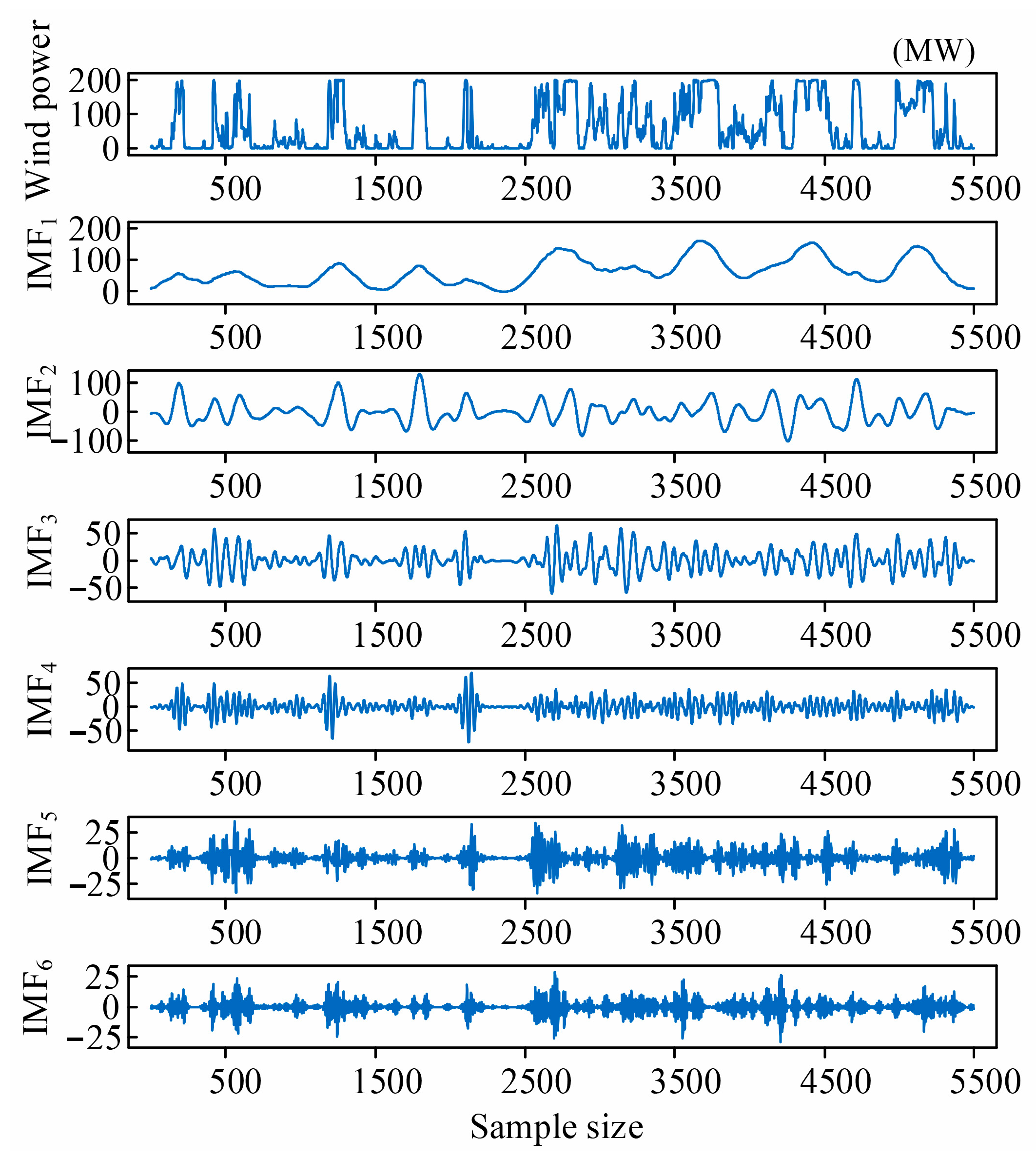
Analysis of modal decomposition sensitivity in Figure 9 demonstrates that prediction error achieves its minimum when K = 6. Consequently, the IVMD results corresponding to this optimal mode number are presented in Figure 10.
As can be seen in Figure 10, the raw wind power data is decomposed into six components that are relatively stable and have different bandwidths, which are used as inputs to the prediction model after combining key meteorological features in turn. When aggregating the forecasts of individual IMF to derive the final wind power prediction, the model presumes statistical independence among IMF forecasting errors. This assumption allows for direct summation of the denormalized IMF forecasts while simplifying the aggregation procedure without compromising predictive accuracy.

5.3. Analysis of Ablation Experiment Results

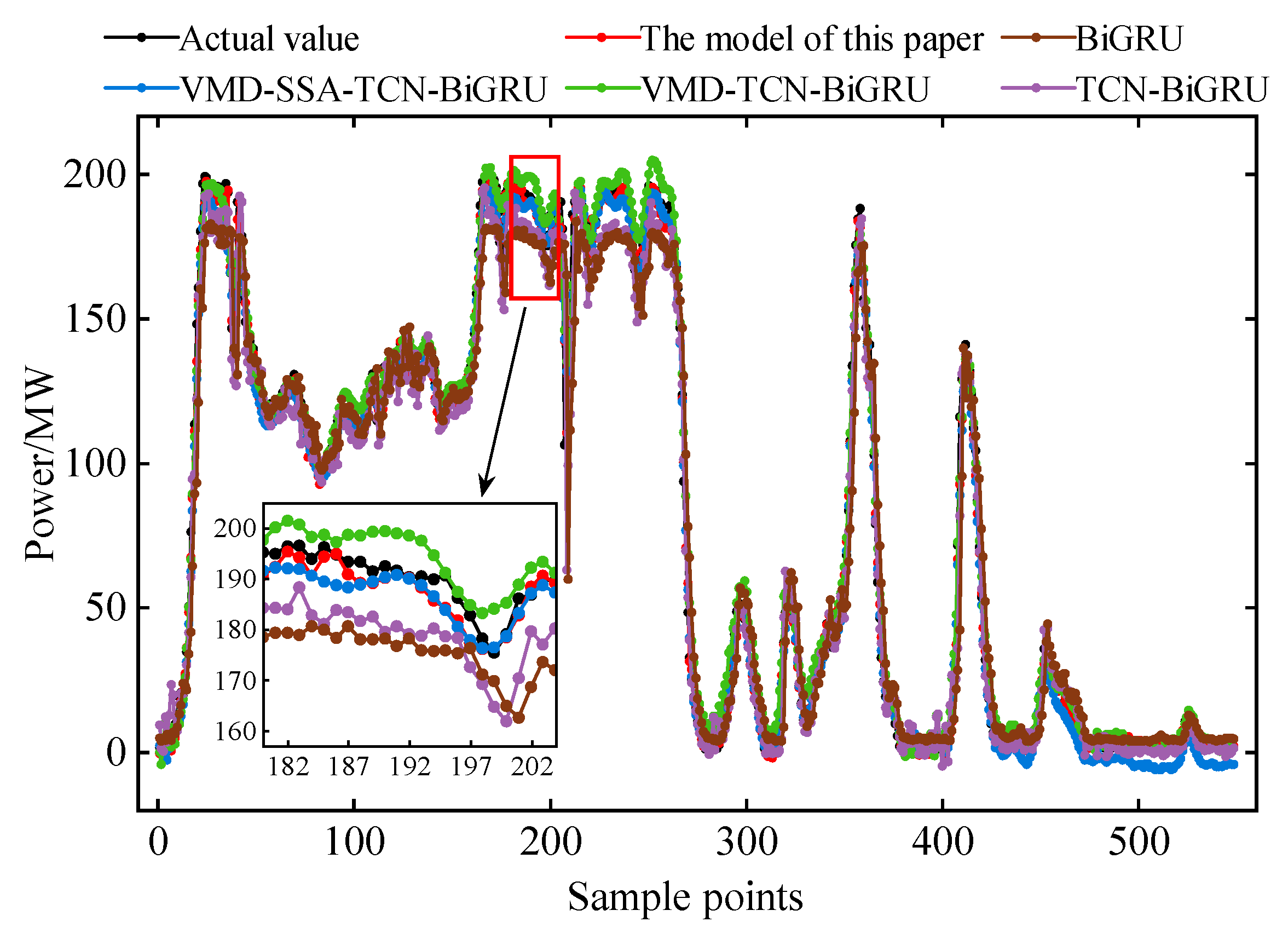
To validate the efficacy of individual modules within the proposed IVMD-SSA-TCN-BiGRU prediction framework, ablation experiments were conducted comparing five configurations: the model of this paper, VMD-SSA-TCN-BiGRU (M1), VMD-TCN-BiGRU (M2), TCN-BiGRU (M3), and baseline BiGRU (M4). The prediction profiles of these models are presented in Figure 11, with corresponding forecasting error metrics quantified in Table 2. It should be noted that for the M1 model, the SSA specifically optimizes the hyperparameters of the TCN-BiGRU architecture, while the parameters of VMD remain at their default settings.
As demonstrated in Figure 11, all five prediction methods generally align with the observed wind power trends. However, the proposed model exhibits superior fidelity to the actual values, particularly during high-volatility periods.
A comparison between the proposed model and the baseline Model M1 demonstrates the necessity of the IVMD-enhanced approach. As presented in Table 2, the proposed method reduces prediction error metrics by 14.94% ( e RMSE ) and 30.88% ( e MAE ), respectively. This improvement indicates that SSA-optimized VMD decomposition of non-stationary wind power sequences into finite-bandwidth IMF submodules effectively enhances prediction accuracy. M1 is the hyper-parameter optimization of the TCN-BiGRU network model using SSA on the basis of M2, resulting in the improvement of e RMSE , e MAE and R 2 by 22.23%, 19.20% and 0.26%, respectively, which demonstrates that the parameter optimization mechanism of SSA is able to effectively improve the effect of the model parameter configurations, and verifies that the traditional empirically-driven parameter setting approach is not able to fully unleash the potential performance advantages of the model. The introduction of VMD decomposition in the M2 model can effectively suppress the noise in the nonlinear wind power series and improve the prediction accuracy, which reduces the value of e RMSE by 26.68% and improves R 2 by 0.63 percentage points compared with the M3 model. The M3 and M4 models can argue for the importance of TCN, with e RMSE and e MAE reduced by 15.75% and 21.40%, respectively, after coupling TCN, indicating that TCN captures global dependencies through convolutional kernels across time steps, which effectively compensates for the problems of insufficient feature mining in the BiGRU module and the forgetting of important information in long sequences.

5.4. Analysis of the Results of Comparative Experiments

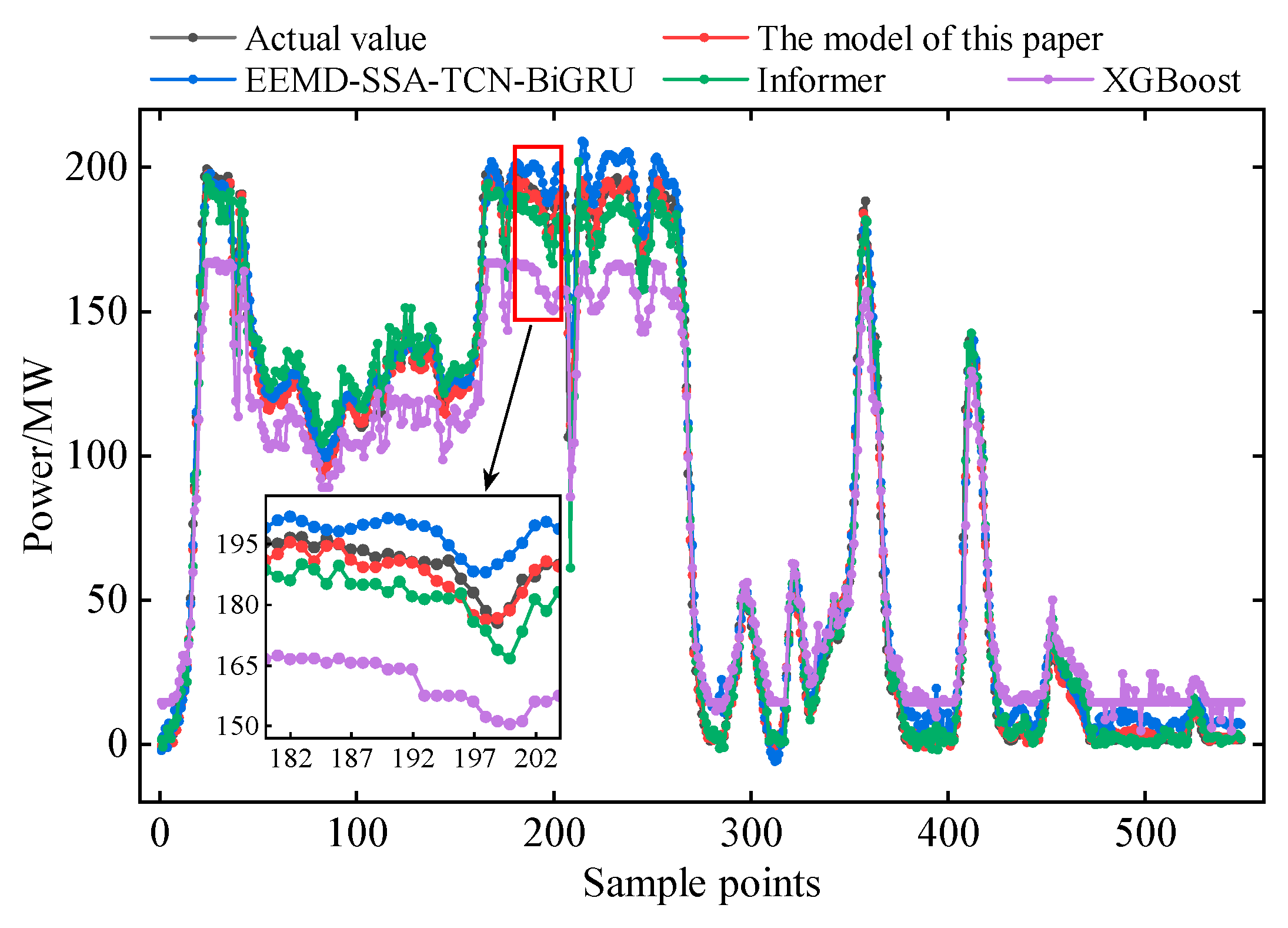
To validate the enhanced robustness of the proposed model for non-stationary sequences, the framework was configured with Table 1 parameters and a batch size of 64. Comparative analysis included the EEMD-SSA-TCN-BiGRU model, the Informer architecture from [35], and the classical XGBoost model. Figure 12 shows the prediction curves of different comparison models, and Table 3 shows the results of the prediction error evaluation of the comparison models.
From the chart, it can be concluded that the results of each model for wind power prediction fluctuate, but the model of this paper has lower errors in all categories. Due to the weak feature extraction ability of the classical XGBoost single model, the prediction error is larger, e MAE is almost 5.74 times that of the model in this paper. Although the implemented Informer model and EEMD-SSA-TCN-BiGRU hybrid model demonstrate enhanced predictive capability relative to conventional models, both exhibit significantly lower performance than the proposed model in this study. Relative to these two methods, the proposed model achieves e RMSE reductions of 39.35% and 36.80%, respectively. This performance disparity may be attributed to the sparse attention mechanism in the Informer model, limiting information utilization efficiency and the introduction of extraneous white noise during the EEMD signal decomposition process.
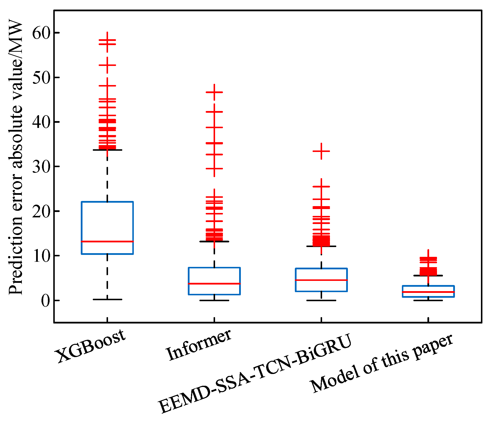
Figure 13 employs boxplots to comparatively visualize absolute prediction error distributions across the four models. The box structure represents the interquartile range (IQR), with upper and lower whiskers denoting the maximum and minimum values within 1.5 × IQR; the central line indicates the median, while “+” symbols mark statistical outliers. Quantitatively, the proposed method demonstrates the narrowest IQR and minimal outlier incidence, validating its enhanced noise suppression and multi-scale feature extraction efficacy.

5.5. Model Generalization Performance Analysis

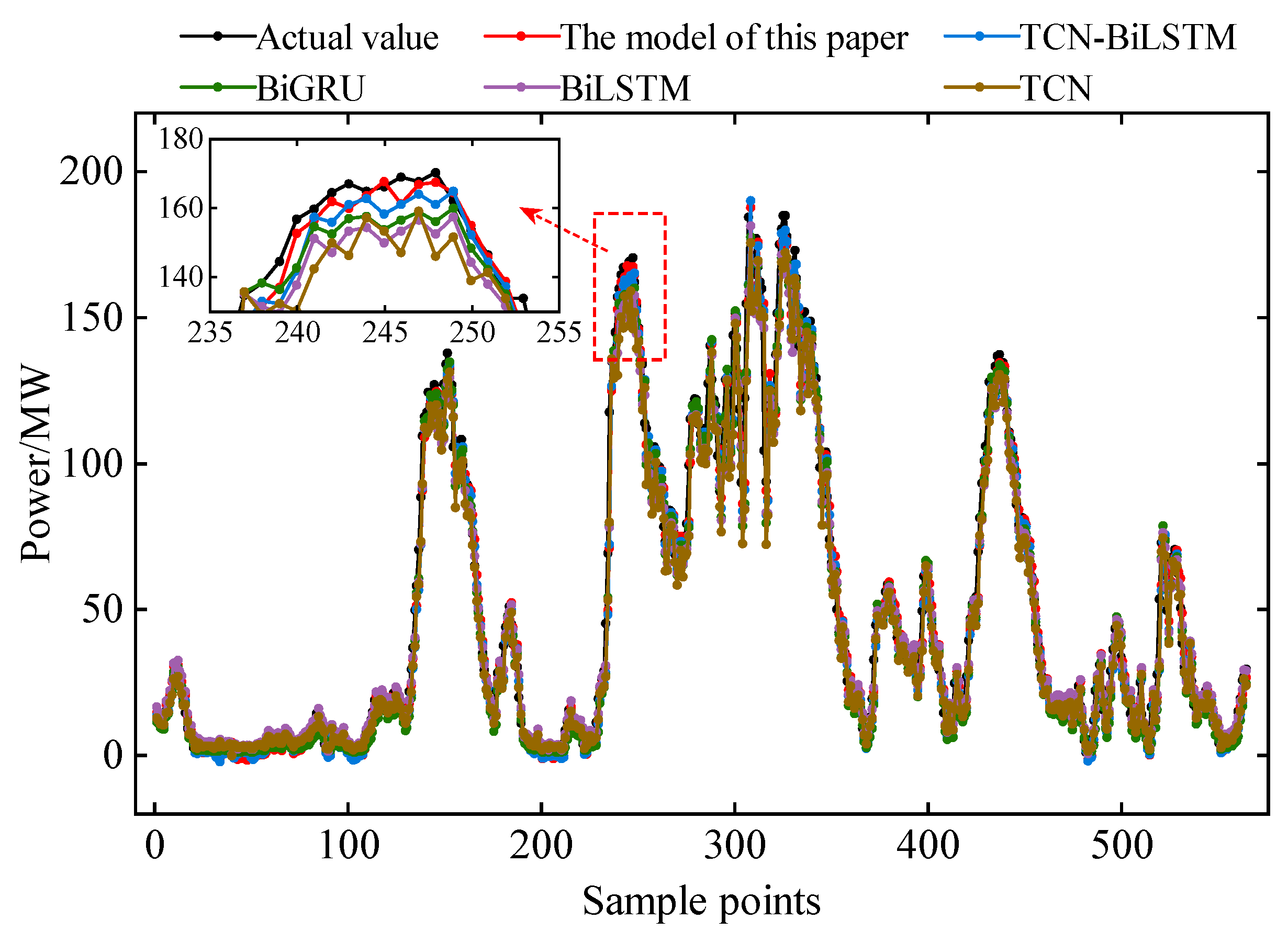
To validate the superior generalization performance of the proposed model, an analysis was conducted using a dataset from another wind farm unit in China. The proposed model was compared with TCN, BiGRU, BiLSTM, and the TCN-BiLSTM hybrid model. The key parameters of all models remained consistent with those specified in Table 1. Figure 14 presents the prediction curves of the aforementioned five models, while corresponding error metric results are summarized in Table 4.
As indicated in Table 4, the proposed model demonstrates relatively higher prediction accuracy compared to the other four deep learning models. Specifically, relative to the standalone TCN model, it achieves reductions of 17.17% and 18.80% in e RMSE and e MAE values, respectively. These results confirm that our model maintains robust generalization performance on wind turbine datasets from a distinct wind farm, further validating its capability to deliver superior prediction accuracy across diverse datasets.

6. Conclusions

To address the non-stationary characteristics of wind power time series and enhance forecasting precision, this paper proposes an ultra-short-term prediction framework integrating IVMD with multi-scale feature extraction. Empirical analysis yields three key findings:
  • The IVMD method adaptively decomposes raw wind power sequences into multiple distinct frequency-band components, significantly reducing the complex non-stationary characteristics in wind power data. This approach reduces e RMSE and e MAE by 14.94% and 30.88%, respectively, compared to non-adaptive benchmark methods in prediction tasks.
  • Within the constructed TCN-BiGRU multiscale feature extraction framework, the TCN captures global trend features through its dilated causal convolution architecture. Concurrently, the BiGRU extracts local detail information via gated recurrent units. Following SSA optimization, the model’s adaptability is further enhanced.
  • Ablation studies demonstrate the critical contributions of each module in the proposed framework, while comparative experiments against three benchmark models confirm its superior performance across all error metrics. These findings substantiate significant deployment potential for ultra-short-term wind power forecasting.
Future studies should incorporate additional influencing factors for wind turbine output, particularly the spatial coordination effects within wind farm clusters. This approach would enhance the data reliability and accuracy critical for power system optimization and dispatch operations.

Author Contributions

Conceptualization, H.W.; methodology, J.S.; software, H.W.; validation, H.W. and C.C.; formal analysis, H.W.; investigation, H.W.; resources, J.S.; data curation, H.W.; writing—original draft preparation, H.W.; writing—review and editing, H.W.; visualization, J.S.; supervision, J.S.; project administration, C.C.; funding acquisition, J.S. All authors have read and agreed to the published version of the manuscript.

Funding

This work was supported by the National Natural Science Foundation of China, grant number 52277012.

Data Availability Statement

The original contributions presented in the study are included in the article; further inquiries can be directed to the corresponding author.

Conflicts of Interest

The authors declare no conflicts of interest.

References

  1. Shu, Y.; Zhao, Y.; Zhao, L.; Qiu, B.; Liu, M.; Yang, Y. Study on Low Carbon Energy Transition Path Toward Carbon Peak and Carbon Neutrality. Proc. CSEE 2023, 43, 1663–1671. [Google Scholar] [CrossRef]
  2. Chen, H.; Li, H.; Kan, T.; Zhao, C.; Zhang, Z.; Yu, H. DWT-DTCNA Ultra-short-term Wind Power Prediction Considering Wind Power Timing Characteristics. Power Syst. Technol. 2023, 47, 1653–1662. [Google Scholar] [CrossRef]
  3. Du, P.; Yang, D.; Li, Y.; Wang, J. An innovative interpretable combined learning model for wind speed forecasting. Appl. Energy 2024, 358, 122553. [Google Scholar] [CrossRef]
  4. Shi, J.; Wang, B.; Luo, K.; Wu, Y.; Zhou, M.; Watada, J. Ultra-short-term wind power interval prediction based on multi-task learning and generative critic networks. Energy 2023, 272, 127116. [Google Scholar] [CrossRef]
  5. Hu, Y.; Zhu, L.; Li, J.; Li, Y.; Zeng, Y.; Zheng, L.; Shuai, Z. Short-term wind power forecasting with the integration of a deep error feedback learning and attention mechanism. Power Syst. Prot. Control 2024, 52, 100–108. [Google Scholar] [CrossRef]
  6. Gong, M.; Yan, C.; Xu, W.; Zhao, Z.; Li, W.; Liu, Y.; Li, S. Short-term wind power forecasting model based on temporal convolutional network and Informer. Energy 2023, 283, 129171. [Google Scholar] [CrossRef]
  7. Guo, N.-Z.; Shi, K.-Z.; Li, B.; Qi, L.-W.; Wu, H.-H.; Zhang, Z.-L.; Xu, J.-Z. A physics-inspired neural network model for short-term wind power prediction considering wake effects. Energy 2022, 261, 125208. [Google Scholar] [CrossRef]
  8. Su, X.; Zhu, M.; Yu, H.; Li, C.; Fu, Y.; Mi, Y. Ultra-short-term probabilistic forecasting of offshore wind power based on spectral attention and non-crossing joint quantile regression. Power Syst. Prot. Control 2024, 52, 103–116. [Google Scholar] [CrossRef]
  9. Xian, H.; Che, J. Unified whale optimization algorithm based multi-kernel SVR ensemble learning for wind speed forecasting. Appl. Soft Comput. 2022, 130, 109690. [Google Scholar] [CrossRef]
  10. Hua, L.; Zhang, C.; Peng, T.; Ji, C.; Nazir, M.S. Integrated framework of extreme learning machine (ELM) based on improved atom search optimization for short-term wind speed prediction. Energy Convers. Manag. 2022, 252, 115102. [Google Scholar] [CrossRef]
  11. Lv, Y.; Hu, Q.; Xu, H.; Lin, H.; Wu, Y. An ultra-short-term wind power prediction method based on spatial-temporal attention graph convolutional model. Energy 2024, 293, 130751. [Google Scholar] [CrossRef]
  12. Zhu, Q.; Li, J.; Qiao, J.; Shi, M.; Wang, C. Application and Prospect of Artificial Intelligence Technology in Renewable Energy Forecasting. Proc. CSEE 2023, 43, 3027–3047. [Google Scholar] [CrossRef]
  13. Kırat, O.; Çiçek, A.; Yerlikaya, T. A new artificial intelligence-based system for optimal electricity arbitrage of a second-life battery station in day-ahead markets. Appl. Sci. 2024, 14, 10032. [Google Scholar] [CrossRef]
  14. Sun, Y.; Zhou, Q.; Sun, L.; Sun, L.; Kang, J.; Li, H. CNN–LSTM–AM: A power prediction model for offshore wind turbines. Ocean Eng. 2024, 301, 117598. [Google Scholar] [CrossRef]
  15. Shahid, F.; Zameer, A.; Muneeb, M. A novel genetic LSTM model for wind power forecast. Energy 2021, 223, 120069. [Google Scholar] [CrossRef]
  16. Harbola, S.; Coors, V. One dimensional convolutional neural network architectures for wind prediction. Energy Convers. Manag. 2019, 195, 70–75. [Google Scholar] [CrossRef]
  17. Zang, H.; Zhao, Y.; Zhang, Y.; Cheng, L.; Wei, Z.; Qin, X. Ultra-short-term Wind Power Prediction Based on Power Correction Under Low Wind Speed and Improved Loss Function. Autom. Electr. Power Syst. 2024, 48, 248–257. [Google Scholar] [CrossRef]
  18. Chen, H.; Zhou, Y.; Wang, C.; Wang, J.; Han, H.; Lü, X. Economic Analysis of System Spinning Reserve Based on Improved CNN-LSTM Short Term Wind Power Prediction. High Volt. Eng. 2022, 48, 439–446. [Google Scholar] [CrossRef]
  19. Chang, Y.; Yang, Z.; Pan, F.; Tang, Y.; Huang, W. Ultra-short-term Wind Power Prediction Based on CEEMDAN-PE-WPD and Multi-objective Optimization. Power Syst. Technol. 2023, 47, 5015–5025. [Google Scholar] [CrossRef]
  20. Xiao, Y.; Zou, C.; Chi, H.; Fang, R. Boosted GRU model for short-term forecasting of wind power with feature-weighted principal component analysis. Energy 2023, 267, 126503. [Google Scholar] [CrossRef]
  21. Yu, M.; Niu, D.; Gao, T.; Wang, K.; Sun, L.; Li, M.; Xu, X. A novel framework for ultra-short-term interval wind power prediction based on RF-WOA-VMD and BiGRU optimized by the attention mechanism. Energy 2023, 269, 126738. [Google Scholar] [CrossRef]
  22. Liu, T.; Qiao, X.; Jian, L.; Jin, C.; Sun, K. TCN Short-term Wind Power Prediction by Introducing Attention Mechanism and Parameter Optimization. Proc. CSU-EPSA 2024, 36, 88–95. [Google Scholar] [CrossRef]
  23. Wu, Y.-K.; Huang, C.-L.; Wu, S.-H.; Hong, J.-S.; Chang, H.-L. Deterministic and probabilistic wind power forecasts by considering various atmospheric models and feature engineering approaches. IEEE Trans. Ind. Appl. 2022, 59, 192–206. [Google Scholar] [CrossRef]
  24. Wang, Y.; Shi, Y.; Zhou, X.; Zeng, Q.; Fang, B.; Bi, Y. Ultra-short-term Power Prediction for BiLSTM Multi Wind Turbines Based on Temporal Pattern Attention. High Volt. Eng. 2022, 48, 1884–1892. [Google Scholar] [CrossRef]
  25. Liu, X.; Pu, X.; Li, J.; Zhang, J. Short-term wind power prediction of a VMD-GRU based on Bayesian optimization. Power Syst. Prot. Control 2023, 51, 158–165. [Google Scholar] [CrossRef]
  26. Zheng, K.; Miao, X.; Lin, Y.; Huang, C. Phase sequence identification method for users in low-voltage transform district with photovoltaic based on maximal information coefficient. Electr. Power Autom. Equip. 2024, 44, 108–114. [Google Scholar] [CrossRef]
  27. Wang, R.; Xu, X.; Lu, J. Short-term Wind Power Prediction Based on SSA Optimized Variational Mode Decomposition and Hybrid Kernel Extreme Learning Machine. Inf. Control 2023, 52, 444–454. [Google Scholar] [CrossRef]
  28. Wang, Q.; Liu, H.; Nie, Z. Two-stage short-term load forecasting based on VMDT-POA-DELM-GPR. Foreign Electron. Meas. Technol. 2024, 43, 101–109. [Google Scholar] [CrossRef]
  29. Wang, H.; Zou, Z.; Li, X.; Wu, Z.; Zhou, K. Short-term wind power prediction based on VMD-ISSA-GRU comprehensive model. Therm. Power Gener. 2024, 53, 122–131. [Google Scholar] [CrossRef]
  30. Yu, W.; Zhu, R.; Chen, X.; Shang, J.; Bai, X.; Wang, H. Phase Sequence Identification Method for Low-Voltage Distribution Stations Area Based on Dual-Scale Similarity and Improved DBSCAN Algorithm. Electr. Power Constr. 2024, 45, 74–88. [Google Scholar] [CrossRef]
  31. Zhao, L.; Liu, Y.; Shen, X.; Liu, D.; Lü, S. Short-term wind power prediction model based on CEEMDAN and an improved time convolutional network. Power Syst. Prot. Control 2022, 50, 42–50. [Google Scholar] [CrossRef]
  32. Liu, S.; Xu, T.; Du, X.; Zhang, Y.; Wu, J. A hybrid deep learning model based on parallel architecture TCN-LSTM with Savitzky-Golay filter for wind power prediction. Energy Convers. Manag. 2024, 302, 118122. [Google Scholar] [CrossRef]
  33. Wang, S.; Shi, J.; Yang, W.; Yin, Q. High and low frequency wind power prediction based on Transformer and BiGRU-Attention. Energy 2024, 288, 129753. [Google Scholar] [CrossRef]
  34. Ni, J.; Zhang, J. Short-term forecasting of integrated energy load in TCN-BiGRU based on multi-task bi-level attention optimization. Control Eng. China 2024, 31, 1924–1936. [Google Scholar] [CrossRef]
  35. Li, L.; Gao, G.; Wu, W.; Wei, Y.; Lu, S.; Liang, J. Short-term Day-ahead Wind Power Prediction Considering Feature Recombination and Improved Transformer. Power Syst. Technol. 2024, 48, 1466–1476. [Google Scholar] [CrossRef]
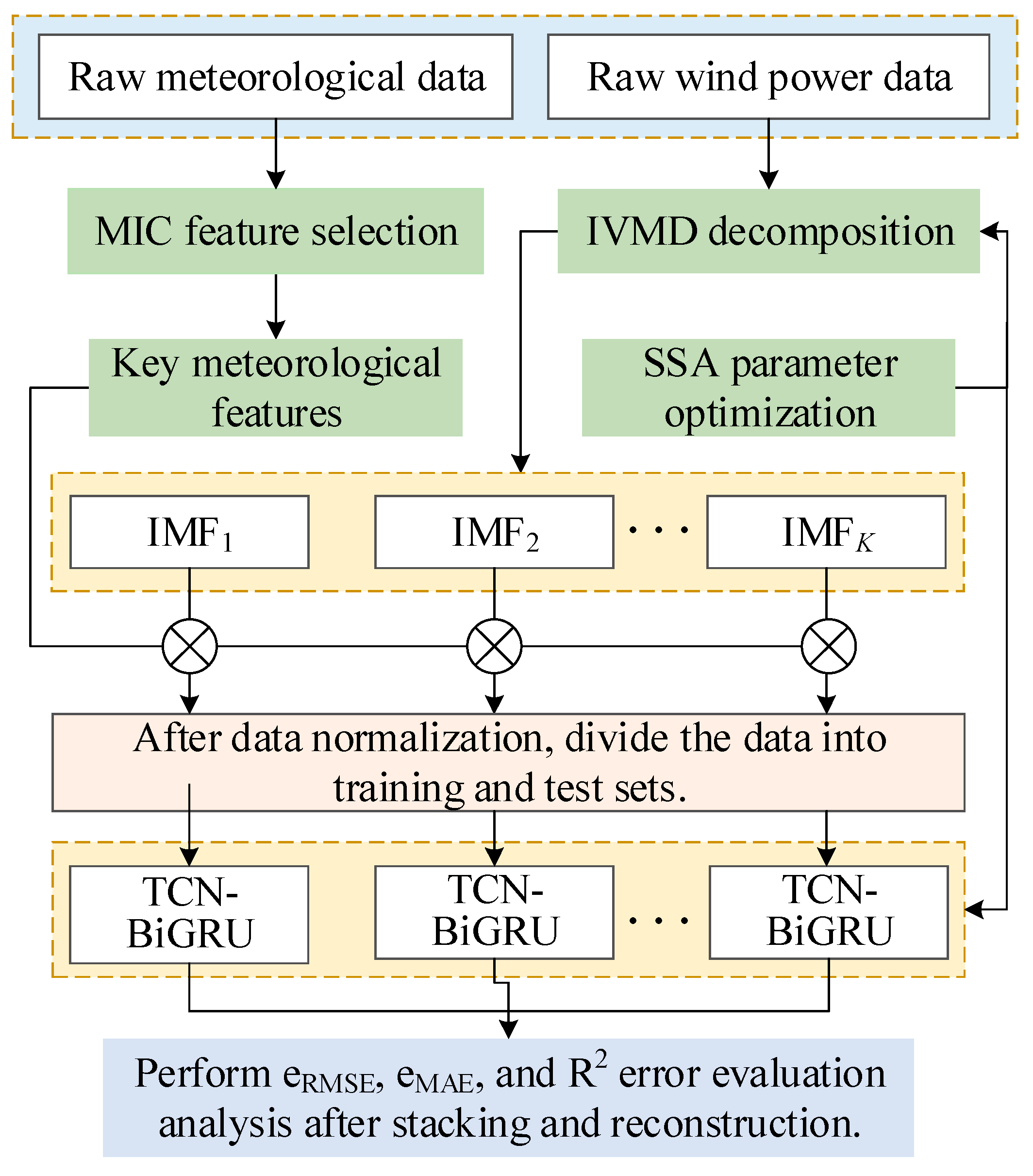
Figure 1. Wind power prediction model architecture.
Processes 13 02606 g001
Figure 2. IVMD flowchart.
Processes 13 02606 g002
Figure 3. TCN structure diagram. (a) Dilated causal convolution; (b) unit residual block.
Processes 13 02606 g003
Figure 4. GRU unit network structure.
Processes 13 02606 g004
Figure 5. BiGRU network architecture.
Processes 13 02606 g005
Figure 6. Network hyperparameter optimization process.
Processes 13 02606 g006
Figure 7. Heat map of MIC analysis for each meteorological factor.
Processes 13 02606 g007
Figure 8. Iterative convergence curve of the algorithm.
Processes 13 02606 g008
Figure 9. VMD modal number sensitivity analysis.
Processes 13 02606 g009
Figure 10. IVMD decomposition results.
Processes 13 02606 g010
Figure 11. Ablation experiment prediction curves.
Processes 13 02606 g011
Figure 12. Comparison of experimental model prediction curves.
Processes 13 02606 g012
Figure 13. Boxplot of the absolute value of error for four prediction models.
Processes 13 02606 g013
Figure 14. Prediction curve of the generalization experiment model.
Processes 13 02606 g014
Table 1. Optimization results of relevant model parameters.
ParametersRealmValue
Modal number of VMD[3–10]6
Penalty factor for VMD[100–2500]2176
TCN convolutional kernel size[2–8]3
TCN convolutional kernel count[32–128]64
learning rate[0.001–0.01]0.003
Regularization factor[0.1–0.3]0.15
BiGRU neuron count[30–135]128
Table 2. Results of prediction error assessment.
ModelsERMSE/MWEMAE/MWR2
M411.0849.1370.97786
M39.3387.1820.98437
M26.8475.1260.99061
M15.3254.1420.99317
The model of this paper4.5292.8630.99550
Table 3. Comparison model prediction error assessment results.
ModelsERMSE/MWEMAE/MWR2
XGBoost18.91016.4310.93564
Informer7.4675.8750.98947
EEMD-SSA-TCN-BiGRU7.1665.6820.98956
The model of this paper4.5292.8630.99550
Table 4. Generalized model error assessment results.
ModelsERMSE/MWEMAE/MWR2
TCN8.2015.3510.97044
BiLSTM7.9035.1190.97626
BiGRU7.6595.1950.97771
TCN-BiLSTM7.3034.8940.97973
The model of this paper6.7934.3450.98272
Disclaimer/Publisher’s Note: The statements, opinions and data contained in all publications are solely those of the individual author(s) and contributor(s) and not of MDPI and/or the editor(s). MDPI and/or the editor(s) disclaim responsibility for any injury to people or property resulting from any ideas, methods, instructions or products referred to in the content.