Abstract
With the rapid pace of urbanization, cities are increasingly facing severe challenges related to environmental pollution, ecological degradation, and climate change. Extreme climate events—such as heatwaves, droughts, heavy rainfall, and wildfires—have intensified public concern about sustainability, environmental protection, and low-carbon development. Ensuring environmental preservation while maintaining residents’ quality of life has become a central focus of urban governance. In this context, evaluating green indicators and predicting urban greenness is both necessary and urgent. This study incorporates international frameworks such as the EU Green City Index, the European Green Capital Award, and the United Nations Sustainable Development Goals to assess urban sustainability. The Extreme Gradient Boosting (XGBoost) algorithm is employed to predict the green level of cities and to develop multiple optimized models. Comparative analysis with traditional models demonstrates that XGBoost achieves superior performance, with an accuracy of 0.84 and an F1-score of 0.81. Case study findings identify “Greenhouse Gas Emissions per Person” and “Per Capita Emissions from Transport” as the most critical indicators. These results provide practical guidance for policymakers, suggesting that targeted regulations based on these key factors can effectively support emission reduction and urban sustainability goals.
1. Introduction
With the rapid development of technology, the emission of greenhouse gases produced by human beings has also risen sharply. Climate change has become more drastic in recent years. In order to mitigate the negative impacts of climate change, countries have been dealing with the issue of climate change through cooperation and conferences, such as the Kyoto Protocol, the Paris Agreement, and the Climate Change Conference. Many countries have also formulated many regulations to improve environmental issues, such as Taiwan’s “Taiwan 2050 Net Zero Emission Pathway and Strategy General Explanation”, which was promulgated in 2022. It provides a trajectory and action pathway to net zero by 2050, with the purpose to promote technology, research, and innovation in key areas, and to guide the green transformation of industries.
In addition to the most widely known term green city/urban, in recent years, there are also related terms such as green innovation [1], green economy [2,3], green logistics [4], urban agriculture/development [5,6], and green building [7]. Since population growth is rapid and most people are concentrated in the urban areas, improving the environment through urban management and resource allocation is very important as a green issue. The United Nations defines a green city as a high quality and environmentally friendly city [8].
Europe is continuously evaluating cities and predicting whether a city is green or not. The European government desires to know whether it meets the criteria for a green city or which indicators are missing. This binary prediction could be made using Logistic Regression. However, it is hard to improve the results with Logistic Regression, since there are not many parameters to be adjusted in the model. In this study, the Extreme Gradient Boosting (XGBoost) tree model [9] along with Logistic Regression are used to make predictions about greenness of cities, where Logistic Regression provides interpretable coefficients that directly convey the direction. XGBoost allows for identification of the most influential predictors in classification tasks (e.g., distinguishing green cities), since it does not provide insight into whether a predictor is positively or negatively associated with the target outcome.
Many different organizations have developed different green city indicators, such as the European Union’s European Green City Index, OECO’s Green Score Index, and GGGI’s Green Growth Index, etc. Professionals working in urban planning, traffic, landscaping, promotion of well-being, and environmental health and protection [10] could be good for city indicator identification. There are some duplicates among the indicators. There are also some uniquely occurring ones. In the real world, there is no unified standard. To recognize which indicators are suitable to a particular area is important. In addition, few studies were developed to evaluate and predict urban greenness, since the data are often incomplete, and the data missing require being resolved.
This study identifies and selects relevant indicators, which are then integrated as input variables for a predictive model. The model is used to analyze the relative importance of each indicator, helping to identify which factors contribute most significantly to a city’s green status. These insights can support governments in prioritizing policy measures and improving urban sustainability based on the most influential indicators.
The European Union (EU) has established many regulations and references regarding green indicators, such as the European Green Capital Award and the European Green City Index [11,12], which are green city awards issued by the EU and the European Green City Index reports of European countries, respectively. This study will mainly refer to European data and use European data for training to predict the data of other countries, as well as to build a prediction model for non-European countries in order to determine the greenness level of cities.
This study aims to achieve three objectives:
- Integrate a new set of green cities indicators by referring to green city indicators in the literature and apply them to predict whether a city is green or not.
- Compare different prediction methods to learn the strengths and weaknesses of the prediction models.
- Recognize the correlation between the indicators and the level of a green city based on the XGBoost and Logistic Regression. The aim of the results is for the government to understand the crucial factors and to improve the greenness level of cities.
2. Literature Review
Section 2.1 reviews existing research on green cities and highlights the limitations and gaps in current studies. Section 2.2 presents a survey of green city indicators, with the goal of identifying and selecting suitable variables to serve as inputs for the predictive model. Finally, prediction models are introduced in Section 2.3.
2.1. Research on Green Cities
The inclusion of climate change on the international political agenda since the early 2000s has elevated the importance of sustainable resource and energy use [13,14]. Alongside this, the image of a city—particularly in terms of environmental governance—has become a key metric in assessing urban sustainability [15]. The United Nations Environment Programme [8] defines a green city as one that is environmentally friendly and meets several key conditions, such as “creating high-quality urban environments for all” and “minimizing the transfer of environmental costs to areas outside the city.” Similarly, scholars describe green cities as urban areas that promote clean air and water, environmentally responsible behavior, and low ecological impacts through public policy [16,17]. Since there is no universally accepted definition, this study draws from multiple perspectives to align definitions with feature categories used in its predictive modeling approach.
Urbanization trends underscore the urgency of green city planning. According to UN data, over half of the global population lived in cities by 2017. This number is expected to increase, with 75% of the global population—around 6.7 billion people—projected to reside in urban areas by 2050. In high-income countries like the U.S., Japan, Australia, and much of Western Europe, urbanization rates have already exceeded 80%. However, urban definitions vary between countries, and some experts argue that existing estimates are likely underreported [18]. Rising urban populations will intensify demands on resources, making efficient planning and sustainable practices critical for the future of cities.
Although numerous studies address environmental issues such as CO2 emissions, waste management, and sustainable transportation [19,20,21,22], relatively few have focused on quantitatively evaluating and predicting the greenness level of cities. Predictive models can provide valuable insights into a city’s environmental performance and identify priority areas for intervention. However, the development of robust models is often hindered by limited data availability, inconsistencies in environmental indicators, and the need to address missing or incomplete values. Overcoming these data challenges is essential for generating actionable insights to support sustainable urban development.
2.2. Indicators of a Green City
Several frameworks have been developed to assess urban sustainability and green performance. The European Green City Index, created by the Economist Intelligence Unit in 2009, evaluates 30 European cities across eight categories: CO2 emissions, energy, buildings, transport, water, waste and land use, air quality, and environmental governance. It includes 13 qualitative and 17 quantitative indicators, shown in Table 1 [12,23]. While qualitative indicators introduce subjectivity, their inclusion is often necessary. Research has also highlighted issues such as inconsistent weighting across categories—for instance, within transportation and energy—which may affect comparability or reflect policy biases [24,25].

Table 1.
The European Green City Index quantitative indicators.
The Green Score Index, developed by the non-profit OECO, is updated quarterly and aims to reflect a city’s environmental footprint in a detailed and practical manner. Although its frequent updates increase relevance, its adoption remains limited due to its nonprofit origins. Selected indicators are listed in Table 2 [26].
Table 2.
Partial Green Score Index.
The Green Growth Index, designed to track progress toward the Sustainable Development Goals (SDGs), the Paris Agreement, and the Aichi Biodiversity Targets, includes metrics on sustainable resource use, economic greening, and social inclusion. However, nearly one-third of its indicators rely on proxy variables, and some countries struggle to meet the data requirements due to technical or environmental constraints, limiting its global applicability [27].
The European Green Capital Award (EGCA) recognizes cities that demonstrate outstanding environmental performance and aims to promote continued improvement. Similarly, this study references the United Nations Sustainable Development Goals, a global framework of 17 objectives adopted by most countries, covering environmental, economic, and social dimensions.
In addition to global frameworks, localized indicators from cities such as Aizawl [28], the Island of Guernsey [29], and several Asian urban centers [30] are also considered. Based on these diverse sources, this study categorizes and analyzes indicator frequency to identify the most relevant variables for inclusion in the predictive model.
2.3. Prediction Model
This study aims to predict whether a city qualifies as “green” or not—a binary classification problem. Logistic Regression is one of the most widely used methods for modeling the relationship between a binary dependent variable and one or more independent variables. It can handle various types of data, including continuous, discrete, dichotomous, ordinal, interval, and ratio variables [31]. However, for more complex classification tasks, decision trees offer a powerful alternative. They do not require linear relationships between variables and are capable of capturing nonlinear interactions [32]. Among tree-based models, Extreme Gradient Boosting (XGBoost)—a supervised learning algorithm based on gradient boosting—has become one of the most popular methods in recent years [33]. Unlike traditional single-model approaches, XGBoost uses an ensemble strategy to iteratively build multiple decision trees (specifically, CART trees), improving model accuracy by correcting the residuals of previous iterations.
XGBoost differs from other ensemble methods like bagging by adopting a sequential learning strategy. While bagging constructs models independently and combines them, boosting builds models sequentially, with each iteration learning from the errors of the previous one. XGBoost further optimizes this process by adding regularization terms to the objective function, reducing the risk of overfitting—a common issue in traditional Gradient-Boosted Decision Trees (GBDTs) [2]. It also incorporates system-level optimizations such as multi-threading via OpenMP and efficient data structures for sparse matrix processing, significantly accelerating training time and scalability [34].
Up-to-date studies show that XGBoost outperforms traditional classification models such as Decision Tree/Random Forest, Support Vector Machines (SVMs), and Neural Networks (NNs) across various domains, including healthcare [35], finance [36], text classification [37], and sustainable development [38]. Its advantages are largely due to gradient boosting, built-in regularization, and efficient handling of missing data [39]. In this study, XGBoost is employed to construct a series of CART trees, where the Gini index is used to determine the optimal feature splits, minimizing classification uncertainty at each node. The final prediction score is the aggregate output from all decision trees, offering improved performance compared to single-model approaches like Logistic Regression. The model’s computational efficiency and predictive power have led to its widespread application across domains, including energy efficiency prediction in buildings [40], pollutant concentration forecasting in environmental science [41], diabetes risk prediction in healthcare [42], and travel time estimation in transportation systems [43].
Given its robustness, scalability, and strong performance in classification tasks, XGBoost is adopted in this study to predict the greenness level of cities based on selected environmental and sustainability indicators.
3. Solution Approach
The solution approach first involves data preprocessing, followed by the training and testing of a Logistic Regression model and Extreme Gradient Boosting (XGBoost) in the data mining process [44]. Feature importance and relevance are calculated, and the results of both are compared to refine the final predictive model.
3.1. Data Pre-Process
Since the collected data still contains some missing values, which cannot be directly used for prediction, it is necessary to perform data imputation to ensure data integrity and check the validity of the data. The kNN algorithm, due to its simplicity and good performance, is widely used in data mining and machine learning. However, this method requires referencing the k nearest values to define the missing values [45]. Given the small sample size in this study, this method is not suitable. Instead, since data from different years was available, the missing values were calculated based on the differences from the previous two years. If no data from other years was available, the mean imputation method was used.
3.2. Evaluation of Green City Indicators
According to the earliest and most comprehensive version of The European Green City Index, the indicators are divided into the following categories: CO2, Energy, Buildings, Transport, Water and Land Use, Air Quality, and Environmental Governance [11,12]. Subsequent green city indicators can also be classified using this framework. Among the recurring indicators are greenhouse gases, CO2 emissions, energy and renewable energy use and generation, green space area, and wastewater management. In the IHS-Green City Conceptual Framework developed by Brilhante and Klaas [15], green space area, wastewater management, and CO2 emissions are given higher weight, and the authors consider them as references for determining livability, aligning with the United Nations’ green standard of creating high-quality urban environments for all. These indicators are also selected as prediction standards in this study, with the main selection criteria being the frequency of occurrence of each indicator in different green city standards (refer to Table 3).
Table 3.
Indicators and descriptions used in this study.
Moreover, due to the difficulty of obtaining complete data, this study primarily focuses on available data or finds similar data as substitutes. Since complete green city indicator data for cities in other regions could not be found, national-level data are used instead. Furthermore, national data are divided by the total population, using per capita data as the final research data to minimize the errors caused by cities and countries. Three indicators are included (Table 3):
- In the transportation category, railway passenger volume, defined as the number of passengers transported by rail multiplied by kilometers traveled, serves as an effective proxy for sustainable urban mobility. High volumes reflect efficient public transit infrastructure, reduced dependency on private vehicles, and lower per capita emissions—all of which align with green city evaluation.
- For water resources, renewable rainwater and river resources are included, as mentioned in the Sustainable Development Goals and the Green Growth Index, using per capita renewable freshwater resources as the standard. The availability and sustainable management of renewable rainwater and river resources reflect a city’s capacity for self-sufficient, low-impact water usage. This criterion supports climate adaptation, reduces carbon footprints related to water supply, and enhances ecological health—key attributes of a green city.
- Finally, due to the increasing severity of climate change in recent years, the European Green Deal and Sustainable Development Goals have also proposed related policies and plans as indicators for climate change measures. Therefore, the degree of disaster risk reduction policies is added as an indicator to assess whether the strategies developed by countries to reduce disaster risk can truly mitigate risks, which is considered a policy-related category in the prediction. The degree of disaster risk reduction (DRR) policy implementation reflects a city’s ability to manage environmental hazards and adapt to climate change. Integrating DRR as a criterion for evaluating green cities underscores the importance of resilience, sustainability, and equitable protection of urban populations and ecosystems.
The training data includes the following indicators: per capita greenhouse gas emissions, per capita CO2 emissions, transport emissions, railway passenger volume, per capita renewable electricity generation, per capita primary energy consumption, proportion of renewable energy, green space area, agricultural land use, proportion of clean water resources, renewable internal freshwater, and the degree of disaster risk reduction policies. These 12 indicators are described and categorized in Table 3 along with their data types.
3.3. XGBoost
XGBoost is a supervised machine learning system for extending the tree boosting algorithm [33]. Given a dataset with n samples and m features, the tree ensemble model outputs , representing the predicted score from all the trees. During the training process, the original model is preserved, and an additional tree is added, effectively introducing another function to correct the shortcomings of the original model. The formula for this is as follows [33,46]:
Note that F represent the space of CART (Classification), Kis the number of regression trees, and denotes the features of sample i. For a given dataset, each leaf node j has an associated prediction score , which can be viewed as the weight of the leaf. The leaf weight is the regression value of all samples at leaf node j in the tree, where and T are the number of leaves in the tree. The final prediction of the model is computed by summing the prediction scores of these leaves [47].
XGBoost aims to converge the objective function to a finite value, where represents the training parameters. is the loss function that measures the model’s fit, while is the regularization term that assesses the model’s complexity [48]. The following is the objective function to be minimized [33]:
represents the loss function, which measures the difference between the predicted values and the target values . The regularization term consists of , which accounts for the complexity cost of introducing additional leaves, λ as the regularization hyperparameter, and , which is the L2 regularization weight of leaf node j [33,47]. However, since XGBoost trains using an additive approach, an additional termis included.
The following is the objective function to be minimized for the i-th case after the t-th iteration [33]:
This study uses the Python version 3.0.0 package XGBClassifier for predictions. The package offers a variety of hyperparameters that can be adjusted to optimize the model. The hyperparameters are described in the table below. After completing the model with default parameters, grid search will be used to select the values that yield the highest average accuracy after cross-validation. Since adjusting all parameters simultaneously is time-consuming, batch grid searches will be conducted. The adjustment order is as follows: first, min_child_weight and max_depth, followed by gamma, then subsample and colsample_bytree, followed by the regularization parameters reg_alpha and reg_lambda, and finally, lowering the learning_rate and increasing n_estimators to complete the model optimization [49,50,51], as shown in Table 4.
Table 4.
Hyperparameters of XGBClassifier.
Additionally, besides using the tree-based model (tree booster) as the primary method in this study, XGBClassifier also offers a linear model-based method (linear booster). This study uses both a tree-based model (tree booster) and a linear-model-based method (linear booster).
3.4. Evaluation Criteria
Each prediction requires different evaluation tools to assess the model’s performance. Among these, AUCs are the most common model validation metrics. Additionally, this study calculates the confusion matrix and several indicators derived from it, such as accuracy, recall, precision, and F1-score, which will be used for model comparison later.
AUC (Area Under the Curve) refers to the area under the ROC curve, which represents the rate of incorrectly predicted positives, i.e., the proportion of instances that were predicted as positive but are actually negative [52,53]. As previously mentioned, the closer the curve is to the top-left corner, the better the result. When the curve is near the top-left corner, the area under the curve is larger, meaning a larger AUC indicates a better model. When the area equals 0.5, the prediction performance is roughly equivalent to random guessing. Therefore, an AUC between 0.5 and 1 is considered a reliable indicator of model performance
The confusion matrix summarizes the data based on the model’s predictions and the actual outcomes. Each row represents the actual condition of the samples, while each column represents the predicted outcomes. The matrix can be divided into four quadrants: True Positive (TP), True Negative (TN), False Positive (FP), and False Negative (FN) [52], as shown in Table 5.
Table 5.
The confusion matrix.
The confusion matrix alone cannot directly determine the quality of a model. Therefore, four metrics derived from the confusion matrix are used to evaluate the model [52,54]:
- Accuracy represents the ratio of correctly predicted cases to the total number of cases. It is not suitable when the proportion of actual cases representing true events is low. The formula is as follows:
- Recall represents the proportion of actual true cases that are correctly predicted as true. This metric is primarily used when the focus is on correctly identifying all true cases, ensuring that no cases are missed. Industries like healthcare often emphasize this metric. The formula is as follows:
- Precision is the proportion of correctly predicted true cases among all cases predicted as true. It is often used when the focus is on the accuracy of positive predictions, such as in situations where the cost of false positives is high. The formula is as follows:
- The F1-score is a combined metric of Precision and Recall. The formula is as follows, where is an adjustable parameter. Ifis 0.5, Precision is more important than Recall; if β is 2, the opposite is true. Ifis 1, Precision and Recall are equally important.
In this study, the goal is to identify all cases that are truly green cities. Therefore, Recall will be selected as the primary metric. The focus is on minimizing the risk of missing any actual green cities, even if it means potentially classifying non-green cities as green.
Recommending cities as green when they do not meet the required environmental standards can lead to several negative consequences. (1) Policy Misguidance: Inaccurate classifications may mislead policymakers into believing that current environmental efforts are sufficient, resulting in complacency or delayed policy interventions [55,56]. (2) Public Misinformation: Labeling non-green cities as green can create a false sense of environmental security among the public, reducing pressure on governments and stakeholders to adopt necessary sustainability measures [57]. (3) Misallocation of Resources: Limited environmental funding or support programs may be wrongly directed to cities that appear to be performing well, while cities in greater need of improvement may be overlooked [58]. (4) Undermining Green Standards: Overestimating environmental performance erodes the credibility of green city certification systems, potentially weakening the legitimacy and trust in future sustainability assessments [59,60]. (5) Inhibiting Progress Toward Environmental Goals: Without accurate assessment, cities may fail to identify key areas for improvement, thus slowing progress toward achieving broader climate change mitigation and sustainable development targets [61,62]. (6) International Reputational Risk: For nations or cities engaged in global environmental reporting or partnerships, false green classification could lead to reputational damage if discrepancies are later revealed [63,64]. Therefore, Recall is an important criteria in green city prediction in this study.
4. Case Study
4.1. Dataset
This study uses the data from Our World In Data [65]. Based on the references, several indicators that have more influence on green cities are selected. Since (1) European countries have more reference indicators in the selection of green cities, and (2) European countries have more comprehensive regulations and selection of green cities, therefore, the data of European countries are selected as the training set, and the test set uses the latest year’s data of other countries. The criteria for determining whether a city is a green city are based on the European Green Capital Award of the European Union (EU). The criteria for judging a green city are based on whether a city in a country is selected as a green city or not. The cities that have been awarded in the last four years are shown in Table 6 [66,67,68,69]. The test set was based on the results of the training and whether or not the city was a green city, with reference to the latest annual ranking of the United Nations’ Sustainable Development Goals. In the training, the lowest ranked city is a threshold. A city higher than this standard was considered a green city.
Table 6.
European Green Capital Award winning cities in the past years.
4.2. Pre-Process
There exist missing data, and the reason is unknow. The occurrence is rare. A simple imputation method was used to fill in missing values. Table 7 below shows the process of imputation using the interpolation method, with the data of The transport emission of Iceland in 2021) on the left representing the dataset before imputation and the data on the right showing the dataset after imputation.
Table 7.
Process of imputation using the interpolation method.
After data pre-processing, the training data consists of 40 records, and the testing data consists of 51 records, with 18 and 20 records labeled as 0 and 1, respectively (Table 8). Here, 0 refers to “Not a Green City” and 1 to “Green City.”
Table 8.
The number of testing and training data after pre-processing.
4.3. Results of Prediction
- XGBoost
To use the XGBClassifier package, parameter tuning is required. In this study, grid search was employed to adjust the parameters according to the sequence and settings mentioned in the research methodology. A 5-fold cross-validation was conducted to calculate the average accuracy score, and the parameter combination with the highest score was selected to build the optimal model. The final result was max_depth = 1, gamma = 0, subsample = 1, colsample_bytree = 0.8, reg_alpha = 0, reg_lambda = 1, n_estimators = 100, and learning_rate = 0.01.
The usage of XGBoost based on both linear and tree models is quite similar, although the parameters differ. For the linear model in this study, the parameters used are alpha and lambda, which correspond to reg_alpha and reg_lambda in the tree model. The optimal parameters, alpha = 1 and lambda = 0.2, were determined through grid search.
Based on the model results, it can be observed that the importance of each indicator varies. The highest importance is assigned to per capita greenhouse gas emissions, followed by per capita carbon dioxide emissions from transportation. The remaining indicators show relatively smaller differences in importance, as illustrated in Figure 1 of the tree-based XGBoost. Since this is a tree model, the relationship between positive and negative correlations cannot be explored, so a comparison with Logistic Regression will be conducted later. Also note that the XGBoost indicator/feature importance scores do not show real statistical correlations or cause-and-effect relationships—they only show how useful each feature is for making predictions.
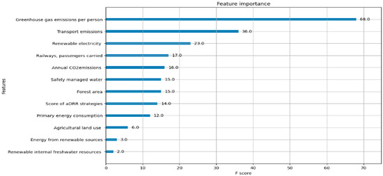
Figure 1.
Importance of indicators in the XGBoost tree model.
- 2.
- Logic Regression
This study aims to recognize the positive and negative correlations of various indicators. Logistic Regression was added for comparison with the previously used XGBoost. During model training, grid search identified the optimal value for the number of iterations, max_iter, as 20, and the value for C as 10. C is the inverse of regularization strength, with larger values indicating weaker control over weights [70].
Based on the correlation coefficients of the Logistic Regression, the positive and negative correlations of the indicators are shown in Figure 2. Comparing this with the indicator importance from the tree model, it can be seen that the two most important indicators are negatively correlated with per capita greenhouse gas emissions and positively correlated with per capita CO2 emissions from transportation. This can be interpreted as representing the extent to which people use public transportation. Therefore, it is necessary to increase the number of buses, railways, and other public transport options.
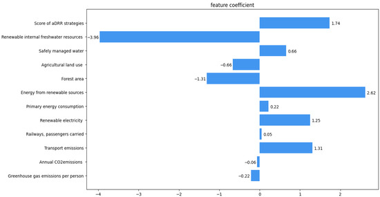
Figure 2.
Correlation of Logistic Regression indicators.
4.4. Comparison and Discussion
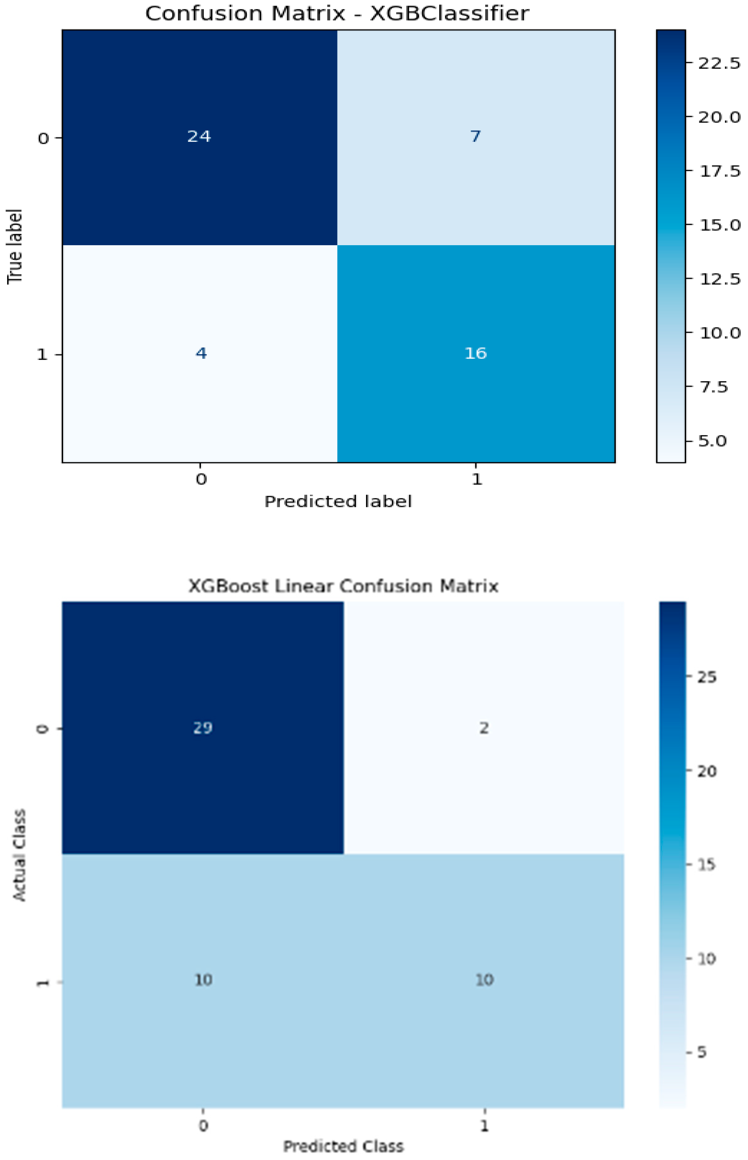
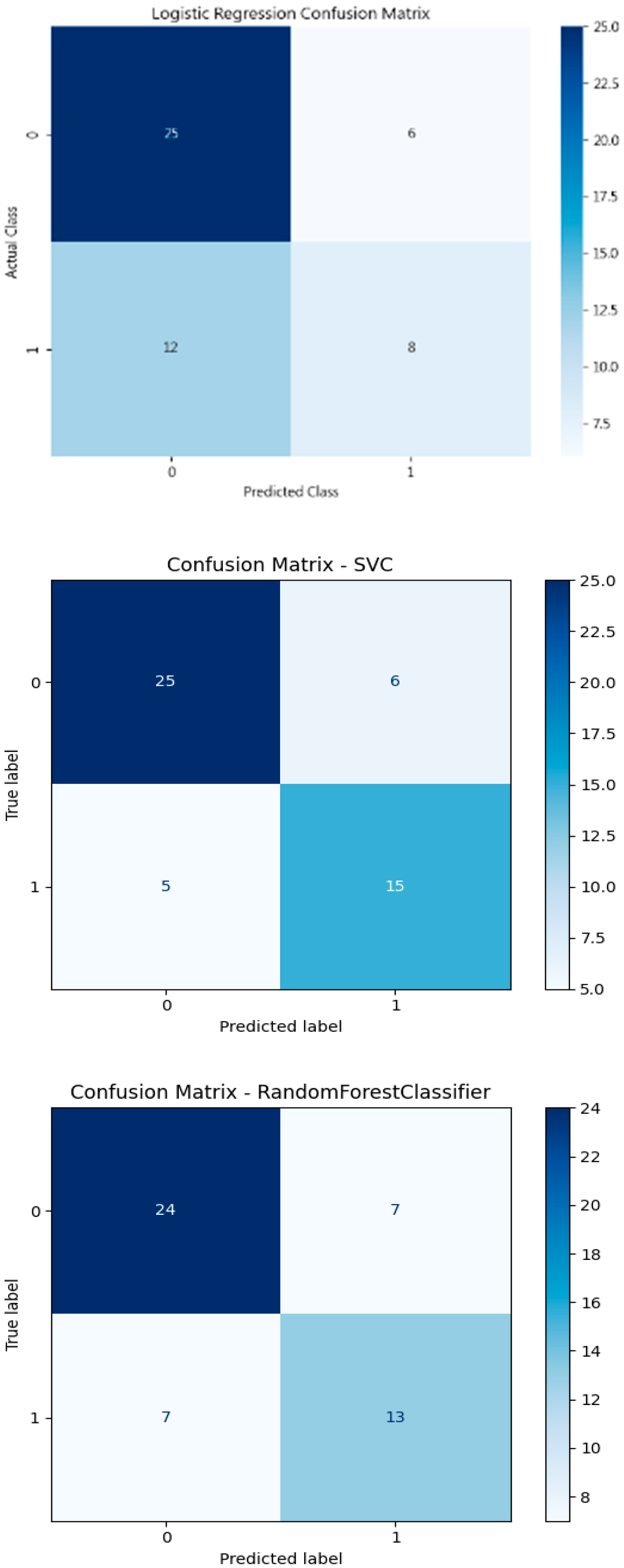
Specifically, classification is a type of prediction problem used to predict categorical outcomes. In this study, six machine learning models are implemented: Logistic Regression (LR), XGBoost with a linear booster (XGBl), XGBoost with a tree booster (XGBt), Random Forest (RF), Support Vector Machine (SVM), and a Neural Network (NN) with one hidden layer of 100 neurons. Figure 3 presents the confusion matrices for these models, each illustrating their performance on a test dataset consisting of 51 samples. The classification task is binary, where Class 1 likely represents areas of “high greenness” and Class 0 represents areas of “low greenness.” Among the test samples, 20 belong to Class 1 and 31 to Class 0. According to the confusion matrix results of the XGBoost tree model (Figure 3), 24 out of 51 observations were accurately classified as non-green cities.


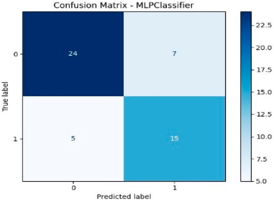
Figure 3.
Confusion matrix results of the models.
Each model’s performance is evaluated based on its ability to correctly classify these instances. A summary of the key evaluation metrics—Accuracy, Recall, Precision, and F1-score—derived from the confusion matrices is provided in Table 9 for comparative analysis. These metrics offer a comprehensive view of how effectively each model predicts urban greenness.
Table 9.
Performance for each model. (Logistic Regression (LR), XGBoost—gblinear (XGBl), XGBoost—gbtree (XGBt), Radom Forest (RF), Support Vector Machine (SVM), Neural Network (NN, one hidden with 100 neurons)).
- XGBt achieved the highest Recall (0.80), indicating its strong ability to correctly identify true positive cases (i.e., correctly classifying green cities). Its F1-score (0.7442) and Accuracy (0.7843) are also the highest among all models, suggesting a good balance between precision and recall as well as overall predictive power. These results indicate that XGBt balances sensitivity (Recall) and Precision effectively, making it the most robust model for predicting green cities.
- The Neural Network model also performs robustly, with an F1-score of 0.71 and a Recall of 0.75, indicating it is effective at identifying green cities while maintaining reasonable precision. The SVC model shows balanced performance as well, slightly outperforming RF in F1-score and Recall.
- In contrast, Logistic Regression shows the weakest performance, with the lowest Recall (0.40), F1-score (0.48), and Accuracy (64.7%). This suggests that while LR provides a simple and interpretable model, it may not capture the complexity of relationships among indicators as well as the ensemble and nonlinear models.
- The XGBl model, while having a lower Recall (0.50), demonstrated the highest Precision (0.83), meaning it is more conservative but reliable when identifying a city as green.
- Overall, tree-based models (XGBt and Random Forest) and Neural Networks show superior predictive capabilities, likely due to their ability to model complex, nonlinear relationships and feature interactions. These findings support the use of advanced machine learning methods—particularly gradient boosting trees—for predicting urban greenness with higher reliability.
Based on the validation indicators and correlation coefficients of each model, we summarize:
- By cross-referencing the feature importance results from XGBoost with the variable correlations from Logistic Regression, each variable can be determined as positively or negatively correlated.
- XGBoost with gbtree emerged as the most effective model, offering a strong balance of Accuracy, Precision, and Recall. It shows superior performance in predicting urban greenness. This finding aligns with the case study conducted by Chen et al. [34]. Similar results have been reported in other domains. For example, in a study on veneer quality prediction in plywood manufacturing, XGBoost achieved comparable Accuracy and Recall to RF and outperformed SVM [71]. In cardiovascular disease prediction using ensemble learning, XGBoost demonstrated higher Precision than RF, SVM, LR, and NN [72]. Additionally, studies on urban forest carbon estimation [73], cropland SOC prediction [74], and a review by Nguyen and Saha [75]—which found that XGBoost outperformed other models, including NN, in 75% of comparisons—further support its superior performance.
- Based on the model results, it is recommended that for predicting green cities, the tree-based XGBoost method should be used to train the model for predicting whether a city is green. However, it is also suggested to use a regression model to understand the correlation coefficients between various indicators. The importance of the indicators and how to improve them to achieve a green city can be determined.
This study derives correlation coefficients among various sustainability indicators. The main findings can be summarized as follows:
- The results of the XGBoost model reveal that Greenhouse Gas Emissions per Person and Transport Emissions are the most influential indicators (Figure 1). These findings are consistent with the existing literature. For instance, [76] recognizes Greenhouse Gas Emissions per Person as a widely adopted benchmark in evaluating national and urban sustainability. Similarly, the United Nations Human Settlements Programme [77] emphasizes this indicator as central to assessing urban sustainability. In addition, Creutzig et al. [78] identified emissions from the transport sector as a major barrier to green development, while the European Environment Agency [18] employed Transport Emissions as a key metric in evaluating urban environmental strategies.
- In a study by [15], which examined correlations between sector-specific green performance and overall green city performance, sanitation and air quality were found to have the highest correlation coefficients. Our results align with this, showing relatively stronger correlations for air-quality-related indicators. In both their findings and ours, energy-related indicators exhibited lower correlation with overall green city classification, particularly in the category of CO2 and energy usage.
- While green initiatives are commonly associated with both energy conservation and carbon reduction, our findings suggest that carbon reduction plays a more critical role. This is reflected in the ranking of top indicators, where Greenhouse Gas Emissions per Person and Transport Emissions per Capita emerge as the two most significant variables, followed by energy-related indicators. The prioritization of carbon metrics over energy consumption implies that cities aiming for green status should emphasize decarbonization strategies.
- Policy-related indicators, such as those measuring disaster risk reduction (DRR), are inherently more difficult to quantify and interpret. Nonetheless, UNDRR [79] provides national- and urban-level scoring frameworks for assessing DRR strategies and benchmarking urban resilience. Likewise, Cardona et al. [80] incorporate DRR strategy implementation as a core metric of sustainability and resilience in urban systems.
- For cities confirmed to be green, quartiles and mean values were calculated (Table 10), and these were used to derive empirical thresholds (Table 11). These thresholds include the following: greenhouse gas emissions of 7.35, carbon dioxide emissions of 11.23, transportation emissions of 1.58, a railway passenger volume of 305,825,000, renewable energy generation of 410.75, primary energy consumption of 42,257.25, proportion of renewable energy of 5.8775, green area of 13,448,250, agricultural land of 7,860,104.5, proportion of clean water resources of 94.1025, renewable inland freshwater of 9970.95, and a disaster mitigation policy level of 0.443. These values can serve as preliminary benchmarks for classifying cities as green or non-green based on objective indicator thresholds. To achieve green city status, it is recommended that governments ensure certain environmental indicators meet or remain below specific thresholds. Among these, per capita greenhouse gas (GHG) emissions is the most critical. Analysis of actual green cities shows that the third quartile value for this indicator is 7.35. Using this value as a threshold yields the highest classification accuracy in identifying green cities. Therefore, it can serve as a practical benchmark. For instance, if a city is predicted—and confirmed—to be non-green, its per capita GHG emissions can be evaluated. If the value exceeds 7.35, policymakers can be advised to prioritize emission reduction strategies. By focusing on this key indicator, cities can more effectively progress toward meeting green city criteria.
Table 10. Mean and quartile values of various indicators in green city data.
Table 11. Number of correct classifications using mean and quartile thresholds in training data.
5. Conclusions
This study applies the Extreme Gradient Boosting (XGBoost) algorithm to evaluate and predict green cities, achieving a high AUC on the test set. Logistic Regression is also employed as a benchmark model to compare predictive performance and provide interpretable feature correlations. XGBoost identifies per capita greenhouse gas emissions as the most important indicator, which also shows a negative correlation in Logistic Regression. Additionally, this study compiles correlation values and threshold levels for key indicators based on actual green city data, offering guidance on performance benchmarks.
While the results demonstrate the effectiveness of machine learning models in classifying green cities and prioritizing influential indicators, several limitations should be acknowledged. First, the sample size of cities may limit the generalizability of the findings across different regions or urban contexts. Second, due to the limited availability of standardized global data, some indicators serve as proxy variables that may not fully capture the complexity of sustainability performance. Third, although feature importance offers valuable insights, it does not imply causality and should be interpreted with caution.
Despite these limitations, the model can serve as a practical decision-support tool. Governments can use this model by inputting city-specific data to assess green status and identify which indicators require improvement. The feature importance rankings generated by the model can help prioritize areas for intervention, enabling more efficient resource allocation and supporting progress toward green city objectives. Ultimately, the broader adoption of such tools can contribute to global environmental sustainability and enhance long-term urban resilience.
Future research includes the following:
- Few studies were developed to evaluate and predict urban greenness, since the amount of data in the dataset is insufficient. Exploring more and consistent data for machine learning is emergent. In the future, larger and more varied datasets are used to make the results stronger and more general.
- The current predictive model still has errors. Future work should explore how to adjust the model or whether other machine learning methods can yield better results.
- Evaluate if there are any missing indicators that should be considered to ensure comprehensive assessment.
- Seek more complete data and further subdivide indicators to enhance accuracy. This will help governments establish clearer standards for achieving green city status.
- Establish separate standards for developing and developed countries. The capacity for investment and the level of infrastructure development vary significantly between these groups, making short-term improvements challenging. Thus, future work should focus on developing green city indicators tailored for developing countries or non-EU governmental authorities.
Author Contributions
Conceptualization, C.-C.H.; methodology, W.-Y.L.; validation, T.-L.T.; data curation, C.-Y.C.; writing—original draft preparation, C.-C.H.; writing—review and editing, W.-Y.L.; All authors have read and agreed to the published version of the manuscript.
Funding
This research was funded by the National Science and Technology Council of Taiwan, grant number (NSTC 113-2410-H-018-035-MY2, NSTC 112-2410-H-260-010-MY3).
Data Availability Statement
Dataset available on request from the authors.
Conflicts of Interest
The authors declare no conflict of interest.
References
- Ma, T.; Wang, S. Green Innovation under the Constraint of Economic Growth Targets: Evidence from Prefecture Level Cities in China. Processes 2023, 11, 1197. [Google Scholar] [CrossRef]
- Zhang, W.; Wu, C.; Zhong, H.; Li, Y.; Wang, L. Prediction of undrained shear strength using extreme gradient boosting and random forest based on Bayesian optimization. Geosci. Front. 2021, 12, 469–477. [Google Scholar] [CrossRef]
- Lucchi, E.; Buda, A. Urban green rating systems: Insights for balancing sustainable principles and heritage conservation for neighbourhood and cities renovation planning. Renew. Sustain. Energy Rev. 2022, 161, 112324. [Google Scholar] [CrossRef]
- Liu, F.P. A Planning Method for City Logistics Considering Carbon Emission and Time Windows. Master Thesis, National Central University, Taoyuan City, Taiwan.
- Freytag, T.; Gössling, S.; Mössner, S. Living the green city: Freiburg’s Solarsiedlung between narratives and practices of sustainable urban development. Local Environ. 2014, 19, 644–659. [Google Scholar] [CrossRef]
- Pham, T.T.H.; Lynch, M.; Turner, S. Creative counter-discourses to the “green city” narrative: Practices of small-scale urban agriculture in Hanoi, Vietnam. Local Environ. 2023, 28, 169–188. [Google Scholar] [CrossRef]
- Qiang, G.; Tang, S.; Hao, J.; Di Sarno, L.; Wu, G.; Ren, S. Building automation systems for energy and comfort management in green buildings: A critical review and future directions. Renew. Sustain. Energy Rev. 2023, 179, 113301. [Google Scholar] [CrossRef]
- UNEP U. Towards A Green Economy: Pathways to Sustainable Development and Poverty Eradication; UNEP: Nairobi, Kenya, 2011. [Google Scholar]
- Xia, W.; Liu, B.; Xiang, H. Prediction of Liquid Accumulation Height in Gas Well Tubing Using Integration of Crayfish Optimization Algorithm and XGBoost. Processes 2024, 12, 1788. [Google Scholar] [CrossRef]
- Suorsa, A.; Multas, A.M.; Rönkkö, E.; Juuti, E.; Lammi, A.; Enwald, H. Information practices in multi-professional work in urban planning. Inf. Res. Int. Electron. J. 2024, 29, 557–572. [Google Scholar] [CrossRef]
- Pace, R.; Churkina, G.; Rivera, M.; Grote, R. How Green is A “Green City”? A Review of Existing Indicators; Karlsruhe Institute of Technology: Karlsruhe, Germany, 2016; Available online: https://publikationen.bibliothek.kit.edu/1000064236 (accessed on 1 August 2025).
- Siemens, A.G. European Green City Index. Assessing the Environmental Impact of Europe’s Major Cities, a Research Project Conducted by the Economist Intelligence Unit, Sponsored by Siemens, Munich. Sponsored by Siemens. 2009. Available online: https://assets.new.siemens.com/siemens/assets/api/uuid:cf26889b-3254-4dcb-bc50-fef7e99cb3c7/gci-report-summary.pdfm (accessed on 1 August 2025).
- Ranaboldo, M.; Aragüés-Peñalba, M.; Arica, E.; Bade, A.; Bullich-Massagué, E.; Burgio, A.; Tani, R. A comprehensive overview of industrial demand response status in Europe. Renew. Sustain. Energy Rev. 2024, 203, 114797. [Google Scholar] [CrossRef]
- Du, X.; Khan, M.N.; Thakur, G.C. Machine Learning in Carbon Capture, Utilization, Storage, and Transportation: A Review of Applications in Greenhouse Gas Emissions Reduction. Processes 2025, 13, 1160. [Google Scholar] [CrossRef]
- Brilhante, O.; Klaas, J. Green city concept and a method to measure green city performance over time applied to fifty cities globally: Influence of GDP, population size and energy efficiency. Sustainability 2018, 10, 2031. [Google Scholar] [CrossRef]
- Kahn, M.E. Green Cities: Urban Growth and the Environment; Brookings Institution Press: Washington, DC, USA, 2007. [Google Scholar]
- Sharifi, A. Co-benefits and synergies between urban climate change mitigation and adaptation measures: A literature review. Sci. Total Environ. 2021, 750, 141642. [Google Scholar] [CrossRef] [PubMed]
- European Environment Agency (EEA). Greenhouse Gas Emissions from Transport in Europe. 2020. Available online: https://www.eea.europa.eu/ims/greenhouse-gas-emissions-from-transport (accessed on 1 July 2025).
- Olivier, J.G.J.; Muntean, M. Trends in Global CO2 Emissions: 2014 Report; PBL Netherlands Environmental Assessment Agency and Institute for Environment and Sustainability of the European Commission’s Joint Research Centre: The Hague, The Netherlands, 2014; Available online: https://www.pbl.nl/en/publications/trends-in-global-co2-emissions-2014-report (accessed on 1 August 2025).
- Santos, G. Road transport and CO2 emissions: What are the challenges? Transp. Policy 2017, 59, 71–74. [Google Scholar] [CrossRef]
- Hannan, M.A.; Begum, R.A.; Al-Shetwi, A.Q.; Ker, P.J.; Al Mamun, M.A.; Hussain, A.; Basri, H.; Mahlia, T.M.I. Waste collection route optimisation model for linking cost saving and emission reduction to achieve sustainable development goals. Sustain. Cities Soc. 2020, 62, 102393. [Google Scholar] [CrossRef]
- Kazancoglu, Y.; Ozbiltekin-Pala, M.; Ozkan-Ozen, Y.D. Prediction and evaluation of greenhouse gas emissions for sustainable road transport within Europe. Sustain. Cities Soc. 2021, 70, 102924. [Google Scholar] [CrossRef]
- Economist Intelligence Unit. The Green City Index: A Summary of the Green City Index Research Series; Economist Intelligence Unit: Munich, Germany, 2012. [Google Scholar]
- Venkatesh, G. A critique of the European green city index. J. Environ. Plan. Manag. 2014, 57, 317–328. [Google Scholar] [CrossRef]
- Wang, X.; Wang, N.; Liu, X.; Shi, R. Energy-saving analysis for the Modern Wing of the Art Institute of Chicago and green city strategies. Renew. Sustain. Energy Rev. 2017, 73, 714–729. [Google Scholar] [CrossRef]
- URL-GS. Available online: https://zero.co.uk/greenscore#:~:text=GreenScore%C2%AE%20is%20a%20number,lower%20impact%20on%20the%20planet (accessed on 1 July 2025).
- Miola, A.; Paccagnan, V.; Papadimitriou, E.; Mandrici, A. Climate resilient development index: Theoretical framework, selection criteria and fit-for-purpose indicators. In JRC Science and Policy Reports; Publications Office of the European Union: Luxembourg, 2015. [Google Scholar] [CrossRef]
- Renthlei, E.; George, A. Toward holistic neighbourhood sustainability assessment: Integrating fuzzy Delphi method for sustainable indicator selection for Aizawl city. Local Environ. 2024, 30, 622–641. [Google Scholar] [CrossRef]
- Mcalpine, P.; Birnie, A. Is there a correct way of establishing sustainability indicators? The case of sustainability indicator development on the Island of Guernsey. Local Environ. 2005, 10, 243–257. [Google Scholar] [CrossRef]
- Krank, S.; Wallbaum, H.; Grêt-Regamey, A. Constraints to implementation of sustainability indicator systems in five Asian cities. Local Environ. 2010, 15, 731–742. [Google Scholar] [CrossRef]
- Mihi, A.; Ghazela, R.; Wissal, D. Mapping potential desertification-prone areas in North-Eastern Algeria using logistic regression model, GIS, and remote sensing techniques. Environ. Earth Sci. 2022, 81, 385. [Google Scholar] [CrossRef]
- Charbuty, B.; Abdulazeez, A. Classification based on decision tree algorithm for machine learning. J. Appl. Sci. Technol. Trends 2021, 2, 20–28. [Google Scholar] [CrossRef]
- Chen, T.; He, T. xgboost: Extreme Gradient Boosting. R Package Version 0.4-2. 2015. Available online: https://cran.r-project.org/web/packages/xgboost/index.html (accessed on 1 August 2025).
- Chen, Z.; Jiang, F.; Cheng, Y.; Gu, X.; Liu, W.; Peng, J. XGBoost classifier for DDoS attack detection and analysis in SDN-based cloud. In Proceedings of the 2018 IEEE International Conference on Big Data and Smart Computing (Bigcomp), Shanghai, China, 15–18 January 2018; IEEE: New York, NY, USA, 2018; pp. 251–256. [Google Scholar] [CrossRef]
- Zhao, Y.; Li, Y.; Li, J.; Wang, Y. Comparative study of XGBoost and other machine learning models for diabetes prediction. Healthcare 2021, 9, 1748. [Google Scholar] [CrossRef]
- Zhang, D.; Zhou, L.; Zhang, D. Credit risk evaluation using machine learning models. Appl. Soft Comput. 2019, 86, 105934. [Google Scholar] [CrossRef]
- Naseem, U.; Razzak, I.; Musial, K.; Imran, M. Transformer based deep intelligent contextual embedding for Twitter sentiment classification. Future Gener. Comput. Syst. 2020, 113, 58–69. [Google Scholar] [CrossRef]
- Li, C.; Zhang, S. Assessing and explaining rising global carbon sink capacity in karst ecosystems. J. Clean. Prod. 2024, 477, 143862. [Google Scholar] [CrossRef]
- Chen, T.; Guestrin, C. XGBoost: A scalable tree boosting system. In Proceedings of the 22nd ACM SIGKDD International Conference on Knowledge Discovery and Data Mining, San Francisco, CA, USA, 13–17 August 2016; pp. 785–794. [Google Scholar] [CrossRef]
- Yan, H.; Yan, K.; Ji, G. Optimization and prediction in the early design stage of office buildings using genetic and XGBoost algorithms. Build. Environ. 2022, 218, 109081. [Google Scholar] [CrossRef]
- Li, J.; An, X.; Li, Q.; Wang, C.; Yu, H.; Zhou, X.; Geng, Y.A. Application of XGBoost algorithm in the optimization of pollutant concentration. Atmos. Res. 2022, 276, 106238. [Google Scholar] [CrossRef]
- Wu, Y.; Zhang, Q.; Hu, Y.; Sun-Woo, K.; Zhang, X.; Zhu, H.; Li, S. Novel binary logistic regression model based on feature transformation of XGBoost for type 2 Diabetes Mellitus prediction in healthcare systems. Future Gener. Comput. Syst. 2022, 129, 1–12. [Google Scholar] [CrossRef]
- Poongodi, M.; Malviya, M.; Kumar, C.; Hamdi, M.; Vijayakumar, V.; Nebhen, J.; Alyamani, H. New York City taxi trip duration prediction using MLP and XGBoost. Int. J. Syst. Assur. Eng. Manag. 2022, 13, 16–27. [Google Scholar] [CrossRef]
- Opesade, A.O. Data mining of Internet users’ interests in diverse, hierarchical information needs. Inf. Res. Int. Electron. J. 2020, 25, 557–572. [Google Scholar] [CrossRef]
- Zhang, S.; Li, X.; Zong, M.; Zhu, X.; Cheng, D. Learning k for knn classification. ACM Trans. Intell. Syst. Technol. (TIST) 2017, 8, 1–19. [Google Scholar] [CrossRef]
- URL-XGB1. Available online: https://cyeninesky3.medium.com/xgboost-a-scalable-tree-boosting-system-%E8%AB%96%E6%96%87%E7%AD%86%E8%A8%98%E8%88%87%E5%AF%A6%E4%BD%9C-2b3291e0d1fe (accessed on 1 July 2025).
- Zhang, D.; Qian, L.; Mao, B.; Huang, C.; Huang, B.; Si, Y. A data-driven design for fault detection of wind turbines using random forests and XGboost. IEEE Access 2018, 6, 21020–21031. [Google Scholar] [CrossRef]
- Huang, J.C.; Tsai, Y.C.; Wu, P.Y.; Lien, Y.H.; Chien, C.Y.; Kuo, C.F.; Kuo, C.H. Predictive modeling of blood pressure during hemodialysis: A comparison of linear model, random forest, support vector regression, XGBoost, LASSO regression and ensemble method. Comput. Methods Programs Biomed. 2020, 195, 105536. [Google Scholar] [CrossRef]
- URL-XGB. Available online: https://xgboost.readthedocs.io/en/stable/python/python_api.html (accessed on 1 July 2025).
- URL-PAR. Available online: https://www.analyticsvidhya.com/blog/2016/03/complete-guide-parameter-tuning-xgboost-with-codes-python/ (accessed on 1 July 2025).
- Torlay, L.; Perrone-Bertolotti, M.; Thomas, E.; Baciu, M. Machine learning–XGBoost analysis of language networks to classify patients with epilepsy. Brain Inform. 2017, 4, 159–169. [Google Scholar] [CrossRef]
- Xu, Z.; Wang, Z. A risk prediction model for type 2 diabetes based on weighted feature selection of random forest and xgboost ensemble classifier. In Proceedings of the 2019 Eleventh International Conference on Advanced Computational Intelligence (ICACI), Guilin, China, 7–9 June 2019; IEEE: New York, NY, USA, 2019; pp. 278–283. [Google Scholar]
- Dhaliwal, S.S.; Nahid, A.A.; Abbas, R. Effective intrusion detection system using XGBoost. Information 2018, 9, 149. [Google Scholar] [CrossRef]
- Kabiraj, S.; Raihan, M.; Alvi, N.; Afrin, M.; Akter, L.; Sohagi, S.A.; Podder, E. Breast cancer risk prediction using XGBoost and random forest algorithm. In Proceedings of the 2020 11th International Conference on Computing, Communication and Networking Technologies (ICCCNT), Kharagpur, India, 1–3 July 2020; IEEE: New York, NY, USA, 2020; pp. 1–4. [Google Scholar] [CrossRef]
- Lee, T.; Lee, H. Collaborative governance and climate change: A case study of Seoul’s metropolitan government. Asian J. Political Sci. 2014, 22, 261–279. [Google Scholar]
- Castán Broto, V.; Bulkeley, H. A survey of urban climate change experiments in 100 cities. Glob. Environ. Change 2013, 23, 92–102. [Google Scholar] [CrossRef]
- Delmas, M.A.; Burbano, V.C. The drivers of greenwashing. Calif. Manag. Rev. 2011, 54, 64–87. [Google Scholar] [CrossRef]
- Anguelovski, I.; Connolly, J.J.; Masip, L.; Pearsall, H. Assessing green gentrification in historically disenfranchised neighborhoods: A longitudinal and spatial analysis of Barcelona. Urban Geogr. 2018, 39, 458–491. [Google Scholar] [CrossRef]
- Sæbø, Ø.; Rose, J.; Flak, L.S. The shape of eParticipation: Characterizing an emerging research area. Gov. Inf. Q. 2020, 27, 265–273. [Google Scholar] [CrossRef]
- Auld, G. Constructing Private Governance: The Rise and Evolution of Forest, Coffee, and Fisheries Certification; Yale University Press: New Haven, CT, USA, 2014. [Google Scholar]
- Bulkeley, H.; Castán Broto, V.; Hodson, M.; Marvin, S. Cities and Low Carbon Transitions; Routledge: Oxfordshire, UK, 2014. [Google Scholar]
- UN-Habitat. World Cities Report 2020: The Value of Sustainable Urbanization; United Nations Human Settlements Programme: Nairobi, Kenya, 2020. [Google Scholar]
- OECD. Compact City Policies: A Comparative Assessment; OECD Green Growth Studies: Paris, France, 2012. [Google Scholar]
- Ghosh, A. False solutions to climate change: How greenwashing undermines climate justice. Globalizations 2020, 17, 1046–1059. [Google Scholar]
- URL-OWD. Available online: https://ourworldindata.org/air-pollution (accessed on 1 July 2025).
- URL-GCA23. Available online: https://environment.ec.europa.eu/topics/urban-environment/european-green-capital-award/winning-cities/tallinn-2023_en (accessed on 1 July 2025).
- URL-GCA22. Available online: https://environment.ec.europa.eu/topics/urban-environment/european-green-capital-award/winning-cities/grenoble-2022_en (accessed on 1 July 2025).
- URL-GCA21. Available online: https://environment.ec.europa.eu/topics/urban-environment/european-green-capital-award/winning-cities/lahti-2021_en (accessed on 1 July 2025).
- URL-GCA. Available online: https://environment.ec.europa.eu/topics/urban-environment/european-green-capital-award_en (accessed on 1 July 2025).
- URL-LOG. Available online: https://scikitlearn.org/stable/modules/generated/sklearn.linear_model.LogisticRegression.html (accessed on 1 July 2025).
- Ramos-Maldonado, M.; Gutiérrez, F.; Gallardo-Venegas, R.; Bustos-Avila, C.; Contreras, E.; Lagos, L. Machine learning and industrial data for veneer quality optimization in plywood manufacturing. Processes 2025, 13, 1229. [Google Scholar] [CrossRef]
- Liu, J.; Dong, X.; Zhao, H.; Tian, Y. Predictive classifier for cardiovascular disease based on stacking model fusion. Processes 2022, 10, 749. [Google Scholar] [CrossRef]
- Uniyal, S.; Purohit, S.; Chaurasia, K.; Rao, S.S.; Amminedu, E. Quantification of carbon sequestration by urban forest using Landsat 8 OLI and machine learning algorithms in Jodhpur, India. Urban For. Urban Green. 2022, 67, 127445. [Google Scholar] [CrossRef]
- Chen, F.; Feng, P.; Harrison, M.T.; Wang, B.; Liu, K.; Zhang, C.; Hu, K. Cropland carbon stocks driven by soil characteristics, rainfall and elevation. Sci. Total Environ. 2023, 862, 160602. [Google Scholar] [CrossRef]
- Nguyen, A.; Saha, S. Machine learning and multi-source remote sensing in forest carbon stock estimation: A review. arXiv 2024, arXiv:2411.17624. [Google Scholar] [CrossRef]
- OECD. Greenhouse Gas Emissions. OECD Environment Statistics. 2020. Available online: https://data-explorer.oecd.org/vis?fs[0]=Topic%2C1%7CEnvironment%23ENV%23%7CAir%20and%20climate%23ENV_AC%23&pg=0&fc=Topic&bp=true&snb=12&df[ds]=dsDisseminateFinalDMZ&df[id]=DSD_AIR_GHG%40DF_AIR_GHG&df[ag]=OECD.ENV.EPI&df[vs]=1.0&dq=.A.GHG._T.KG_CO2E_PS&pd=2014%2C&to[TIME_PERIOD]=false (accessed on 1 July 2025).
- UN-Habitat. Hot Cities: Battleground for Climate Change. United Nations Human Settlements Programme. 2011. Available online: https://unhabitat.org/sites/default/files/2012/06/P1HotCities.pdf (accessed on 1 July 2025).
- Creutzig, F.; Jochem, P.; Edelenbosch, O.Y.; Mattauch, L.; van Vuuren, D.P.; McCollum, D.; Minx, J. Transport: A roadblock to climate change mitigation? Science 2015, 350, 911–912. [Google Scholar] [CrossRef]
- UNDRR. Annual Report 2022. Available online: https://www.undrr.org/media/87504/download?startDownload=20250709 (accessed on 9 July 2025).
- Cardona, O.D.; Ordaz, M.; Reinoso, E.; Yamín, L.E.; Barbat, A.H. CAPRA–Comprehensive Approach to Probabilistic Risk Assessment: International Initiative for Risk Management Effectiveness. In Proceedings of the 15th World Conference on Earthquake Engineering, Lisbon, Portugal, 24–28 September 2012; Volume 1. [Google Scholar]


Disclaimer/Publisher’s Note: The statements, opinions and data contained in all publications are solely those of the individual author(s) and contributor(s) and not of MDPI and/or the editor(s). MDPI and/or the editor(s) disclaim responsibility for any injury to people or property resulting from any ideas, methods, instructions or products referred to in the content. |
© 2025 by the authors. Licensee MDPI, Basel, Switzerland. This article is an open access article distributed under the terms and conditions of the Creative Commons Attribution (CC BY) license (https://creativecommons.org/licenses/by/4.0/).