Abstract
In response to the low efficiency of collaborative processing of sewing machine cases at the part level in network collaborative manufacturing, this paper proposes a sewing machine cases manufacturing service composition optimization method based on an improved multi-objective artificial hummingbird algorithm. The structure and production process of sewing machine cases are analyzed; a framework for service composition optimization in the sewing machine cases manufacturing service platform is established; the required manufacturing resource service composition is determined; and a dual-objective service composition optimization mathematical model that considers Quality of Service (QoS) indicators and flexibility indicators is constructed. Opposition-based learning strategies, roulette wheel selection strategies, and improved differential evolution strategies are embedded in the multi-objective artificial hummingbird algorithm, and the improved artificial hummingbird algorithm (ORAHA_DE) is used to solve the sewing machine cases manufacturing service composition optimization model. The experimental results show the effectiveness and superiority of this composition optimization method in solving the sewing machine cases manufacturing composition optimization problem while avoiding entrapment in a local optimum during the solution process, thereby achieving the composition optimization of sewing machine cases collaborative manufacturing services.
1. Introduction
Sewing machine cases are the benchmark components for sewing equipment assembly, and their processing and assembly accuracy directly determine the quality and service life of sewing equipment. However, traditional processing methods for sewing machine cases suffer from problems such as scattered manufacturing resources and insufficient industrial coordination, which seriously hinder the high-quality development of sewing equipment manufacturing enterprises in the cluster area and constrain the production efficiency of sewing equipment. Network collaborative manufacturing is an advanced manufacturing model based on information technology and the Internet. It is a new type of intelligent manufacturing model that integrates the resources, information, and technology of upstream and downstream enterprises in the supply chain to achieve collaborative manufacturing and management, thereby improving production efficiency and reducing costs [1,2,3]. The use of collaborative manufacturing to achieve the intelligent transformation of sewing machine cases production is an inevitable trend in the development of the sewing equipment manufacturing field [4]. Through the collaborative manufacturing platform, manufacturing resources and service demands can be intensively integrated to achieve the optimal allocation of resources in the sewing machine cases manufacturing industry and shorten the sewing machine cases manufacturing cycle [5,6].
In a collaborative manufacturing environment, research on resource combination optimization methods is crucial for the implementation and development of collaborative manufacturing. Liu et al. [7] proposed a new method combining an extensible clustering algorithm with fuzzy hierarchical analysis to address the difficulty of optimizing the composition of guided roller cloud manufacturing services. Fazeli et al. [8] combined the characteristics of multiple heuristic algorithms to propose a flexible and scalable resource composition optimization method, which achieved the recommendation of optimal resource composition schemes. Hu et al. [9] proposed a two-stage method for optimizing service composition in a cloud manufacturing environment to achieve resource composition optimization. Cai et al. [10] proposed an improved multi-center vortex search algorithm for global optimization of service composition problems to address the problem of the standard vortex search algorithm easily falling into local minima. Song et al. [11] proposed a cloud-edge collaboration-based cloud manufacturing service composition optimization framework that considers manufacturing service uncertainty to simulate service uncertainty. Rodriguez et al. [12] proposed a hybrid method for automatically composing network services to minimize the number of services generated. The difficulty of manufacturing service composition optimization mainly lies in the construction of the composition optimization model and the solution of the model, which determines the quality of collaborative manufacturing services and whether the manufacturing service process can be carried out smoothly and efficiently.
In terms of service composition optimization model construction, Sodhro et al. [13] proposed a new adaptive QoS calculation algorithm (AQCA) for fair and efficient monitoring of performance indicators in medical data processing in medical applications. Badawy et al. [14] proposed a dynamic QoS provisioning framework for the service-oriented IoT, which maximizes the overall service quality at the IoT application layer by balancing the acceptable cost of service reliability and computation time. Sun et al. [15] proposed a QoS-guaranteed path selection algorithm that selects QoS-guaranteed routing paths for data streams with different QoS requirements. Yu et al. [16] developed a prediction model using the similarity characteristics of time QoS values and used this model to comprehensively consider QoS attributes and candidate services, confirming that this method can find better services by reducing misjudgments of user preferences. However, when solving the problem of manufacturing service composition optimization, most current studies focus on evaluation indicators such as time, cost, and quality, without considering the flexibility indicators that are important to manufacturing resource providers.
In terms of service composition optimization model solving, meta-heuristic algorithms are widely used to solve manufacturing service composition optimization problems. They include, for instance, the multi-objective genetic algorithm (NSGA-II) [17], the multi-objective genetic algorithm (NSGA-III) [18], the multi-objective particle swarm optimization algorithm [19], the multi-objective gray wolf optimization (MOGWO) algorithm [20], the multi-objective artificial hummingbird optimization algorithm (MOAHA) [21], the multi-objective grasshopper optimization algorithm (MOGOA) [22], and the multi-objective differential evolution (MODE) algorithm [23]. At present, many studies based on algorithmic solutions to service composition optimization problems have been conducted both domestically and internationally. Gao et al. [24] proposed an improved polar bear optimization algorithm to solve the problem of low efficiency in the outsourcing of coating machine wall panel parts in a network collaborative manufacturing model. Li et al. [25] proposed a service composition optimization method based on the extended Gale–Shapley algorithm, which realized the optimal recommendation of manufacturing service composition and met the manufacturing needs of the manufacturing demand side. Zhang et al. [26] proposed an optimization algorithm WS FOA (Web Service composition based on Fruit Fly Optimization Algorithm) for service composition based on service composition modeling and the FOA (Fruit Fly Optimization Algorithm). Zhang et al. [27] established a multi-objective service sharing optimization model and proposed a multi-objective algorithm based on particle swarm optimization to address service composition issues sensitive to service level agreements. Yang et al. [28] proposed a new dynamic ant colony genetic hybrid algorithm to enhance accuracy and stability when addressing large-scale cloud service composition and optimization issues. Seghir [29] proposed a fuzzy discrete multi-objective artificial bee colony method to solve multi-objective service quality-driven network service composition problems. However, in actual manufacturing, most existing multi-objective optimization model solution schemes are not applicable to solving complex models of sewing machine cases manufacturing resource information.
In summary, there are still some key issues in the service composition optimization of sewing machine cases manufacturing:
- Many multi-objective optimization algorithms lack sufficient optimization capabilities when solving manufacturing resource service combination optimization problems and are prone to falling into local optima.
- Sewing machine cases are manufacturing equipment with relatively complex characteristic information, and an optimal model for the complex service composition of sewing machine cases has not yet been fully established.
In response to the above issues, this paper proposes a sewing machine cases manufacturing service composition optimization method based on the ORAHA_DE algorithm.
Based on field research of manufacturing enterprises, the sewing machine cases production process and structure were summarized; the sewing machine cases parts manufacturing subtasks were sorted out; a sewing machine cases manufacturing service composition optimization evaluation indicator system was established; and a dual-objective service composition optimization mathematical model considering QoS indicators and flexibility indicators was established. The ORAHA_DE algorithm was used to solve the service composition optimization mathematical model and obtain the optimal manufacturing service composition plan.
2. Materials and Methods
2.1. Materials
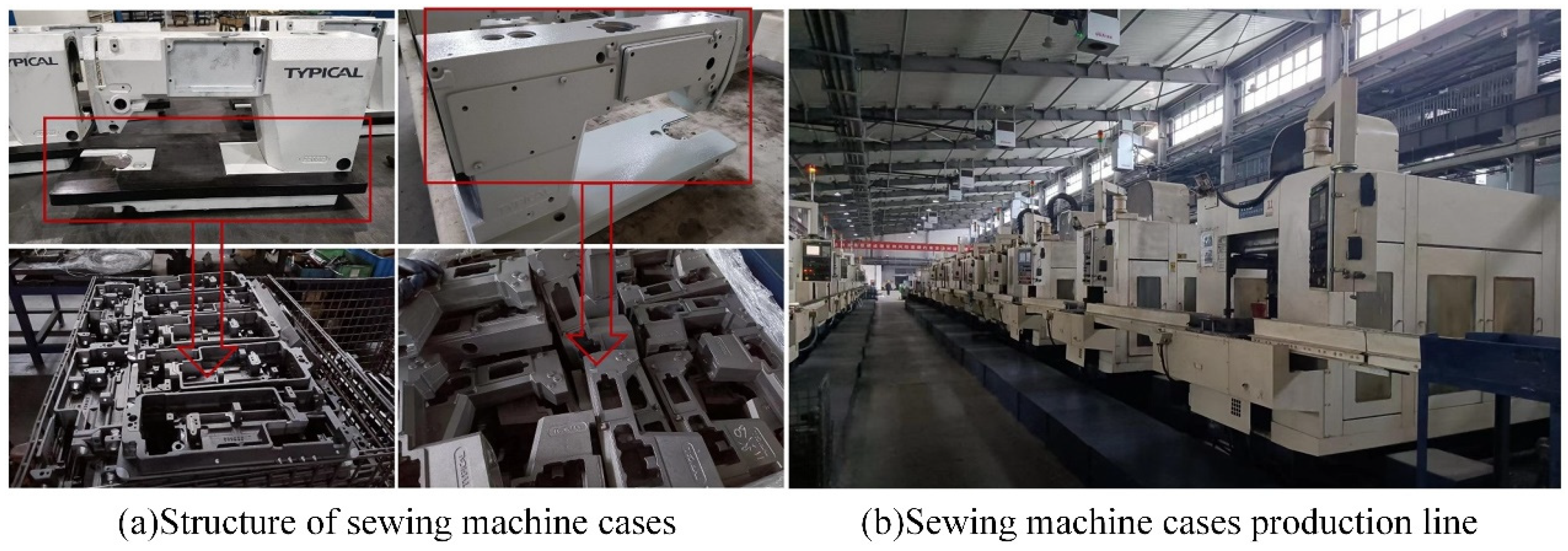
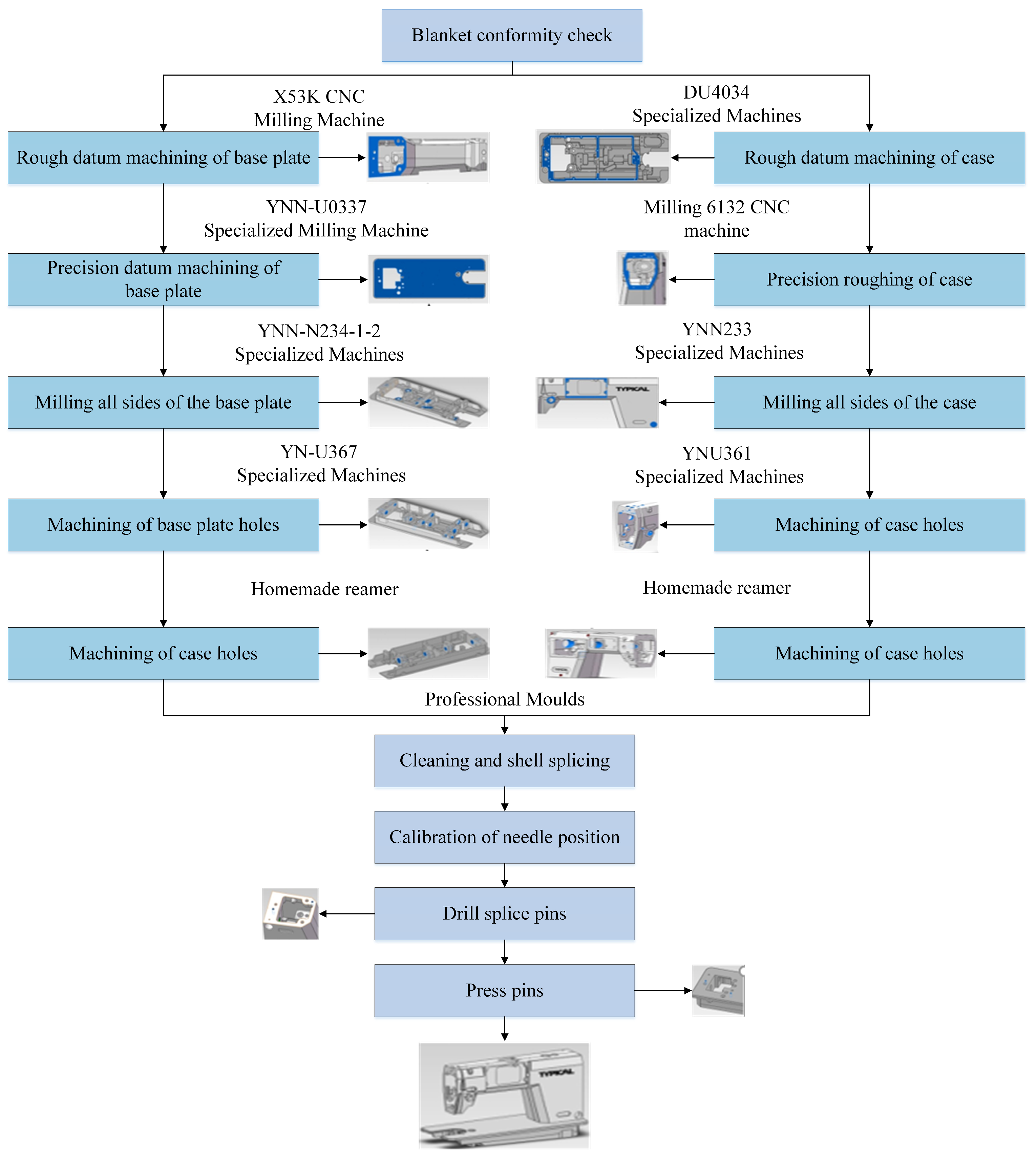
This paper takes sewing machine cases as the research object, combines industrial field research, as shown in Figure 1, and sorts through relevant machine tool processing literature [30,31] to summarize the fine processing and assembly processes of sewing machine cases. Sewing machine cases consist of two parts: the head and the base plate. Their production requires a series of complex and special processing techniques, including blank conformity inspection, rough reference processing of the case and base plate, fine reference processing of the case and base plate, milling of all sides of the case and base plate, processing of holes in the case and base plate, tapping the reference holes of the case and the reference holes of the base, cleaning and assembling the case, calibrating the needle position, drilling the joint pins and drilling the crimping pins, and 10 other major processes, as shown in Figure 2.

Figure 1.
Structure of sewing machine cases and production line conditions.
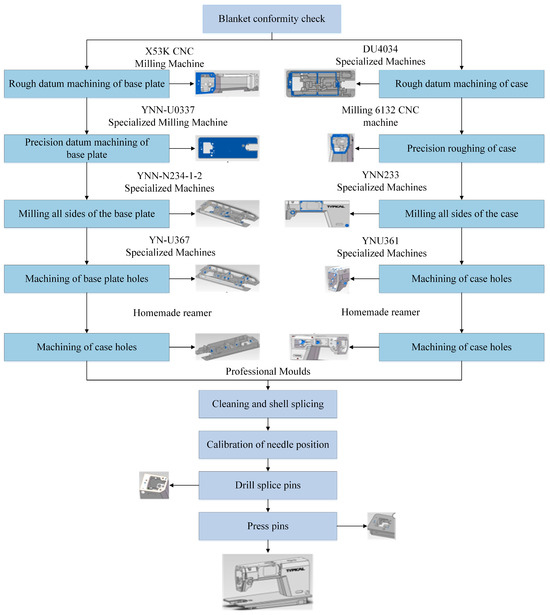
Figure 2.
Sewing machine cases processing technology and structure.
2.2. Classification of Manufacturing Tasks
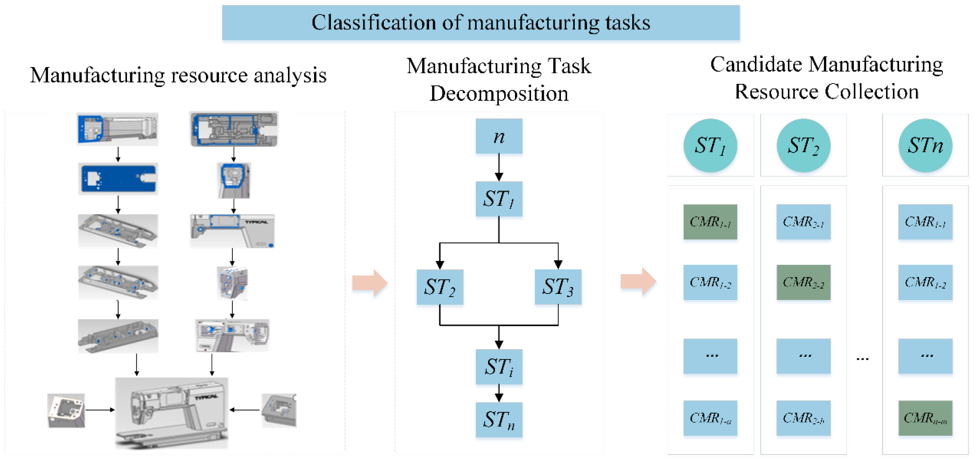
In a collaborative manufacturing environment, dispersed manufacturing service units are arranged according to established specifications and processes and combined into composite services with comprehensive capabilities to achieve complex manufacturing tasks and complete collaborative manufacturing service compositions. Taking the production of sewing machine cases as an example, numerous process-level manufacturing services are combined into part-level manufacturing services to achieve accurate matching and efficient allocation of sewing machine cases resources.
Manufacturing demand is characterized by continuity and a high degree of customization. After the demand side submits a task on the platform, the system will break it down into a series of sub-tasks based on the part process route, generate a number of candidate service sets for each sub-task, and select the best services from the respective candidate sets based on the platform, ultimately forming a globally optimal service composition plan. The manufacturing task classification process is shown in Figure 3.

Figure 3.
Manufacturing task classification process.
When the collaborative manufacturing platform receives a manufacturing request submitted to the service requester, the manufacturing request is decomposed into n subtasks (ST1, ST2, …, STi, …, STn). For each decomposed subtask STi, there are m manufacturing resources that can meet the requirements. For subtask STi, the corresponding candidate manufacturing resource set is CMRi = {CMRi-1, CMRi-2, …, CMRi-m}.
2.3. Evaluation Indicator System for Manufacturing Service Composition Optimization
In the process of realizing collaborative manufacturing of sewing machine cases, the collaborative manufacturing platform management, service demand side, and service provider side are the three core entities that jointly participate in and determine the optimal results of the manufacturing service composition. The reasonable construction of the evaluation indicator system is a prerequisite for ensuring the realization of the optimal manufacturing service composition process. The manufacturing service demand side is more concerned with indicators such as the time, cost, quality, and historical reputation required for manufacturing services, that is, the QoS indicators of the manufacturing resource service composition. However, in a collaborative manufacturing environment, manufacturing tasks are easily affected by changes in manufacturing tasks and manufacturing resources, which in turn affects the efficiency of completing manufacturing tasks. Therefore, it is necessary to incorporate flexible indicators into the factors that need to be considered in the manufacturing resource composition optimization process, namely, the ability of collaborative manufacturing service providers to respond to changes in case manufacturing tasks and manufacturing resources, as well as service evaluation indicators. The evaluation indicator system for manufacturing service composition optimization is shown in Figure 4.
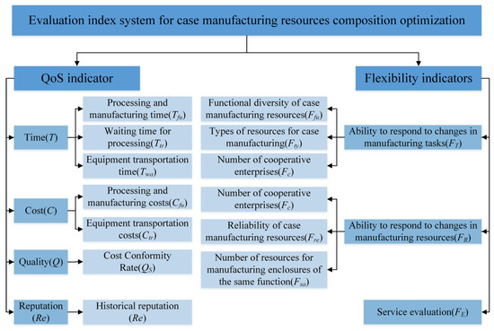
Figure 4.
Evaluation indicator system for service composition optimization of sewing machine cases manufacturing resources.
The QoS indicators for the optimization evaluation indicator system of sewing machine cases manufacturing resource service composition optimization include time T, cost C, quality Q, and reputation indicator Re. The specific details are as follows:
- Time indicator T: Includes processing and manufacturing time Tfu, processing waiting time Ttr, and equipment transportation time Twa.
- Cost indicator C: Includes processing and manufacturing costs Cfu and equipment transportation costs Ctr.
- Quality indicator Q: Refers to the quality acceptance rate of manufacturing service providers completing relevant manufacturing tasks, expressed as Qs.
- Reputation indicator Re: Used to indicate the historical reputation of manufacturing services.
The flexible indicators of the service composition optimization evaluation indicator system for sewing machine cases manufacturing resources include the manufacturing service provider’s ability to respond to changing manufacturing tasks FT, ability to respond to changing manufacturing resources FR, and service evaluation FE. The specific details are as follows:
- Ability to respond to changes in manufacturing tasks FT: Refers to the ability of manufacturing resource providers to successfully complete manufacturing tasks even when the content of the tasks changes after they have been assigned. The quality of this ability directly affects the efficiency of manufacturing resource composition optimization, so it is included in the flexibility indicators. The ability to respond to changes in manufacturing tasks includes the diversity of manufacturing resource functions Ffu, the types of manufacturing resources Fty, and the number of cooperating enterprises Fc.
- Manufacturing resource change response capability FR: Refers to the ability of the manufacturing resource provider to successfully complete a manufacturing task after it has been assigned, even if the manufacturing resources participating in the manufacturing service withdraw from the service for some reason. The quality of this ability directly affects the stability of completing manufacturing tasks in the process of manufacturing resource composition optimization, so it is included in the flexibility indicators, including the number of cooperative enterprises Fc, the reliability of manufacturing resources Fre, and the number of manufacturing resources with the same function Fsa.
- Service evaluation FE: This refers to the historical service evaluation of various manufacturing resources, that is, the satisfaction evaluation given by service demanders to the provision of manufacturing resources during the manufacturing service process. It represents the service attitude, service capacity, service level, speed of problem handling, quality of problem handling, and attitude toward problems of manufacturing services. The higher the service evaluation, the stronger the ability of manufacturing services to respond to changes in manufacturing tasks and manufacturing resources. Therefore, service evaluation is included in the soft indicators.
2.4. Consideration of a Dual-Objective Service Composition Optimization Model with QoS Indicators and Flexibility Indicators
Given that the value ranges of each attribute in the QoS metrics differ, it is necessary to normalize the values of each metric before calculating the overall QoS value. Based on their practical significance, QoS attribute metrics are categorized into positive attribute metrics and negative attribute metrics [32]. The larger the positive attribute value, the better the quality of the service chain; quality Q and service reliability Re are positive attributes. The smaller the negative attribute value, the better the quality of the service chain; time T and cost C are negative attributes. As shown in Equation (1), the four attributes can be normalized to the range [0, 1].
where emax and emin are the maximum and minimum values of the evaluation indicators, respectively. When emax = emin, qk = 1.
In the problem of service portfolio optimization, a manufacturing service portfolio is composed of multiple individual services aggregated together. The aggregation method is related to the task structure, and there are four common types of task structures: sequential structure, parallel structure, selection structure, and cyclic structure. Before evaluating the various attributes of the manufacturing service composition, the QoS attributes of the manufacturing cloud service need to be aggregated according to these four structures, and the attribute values of the complete service composition need to be calculated. Based on this analysis, this paper constructs a series model QoS aggregation calculation framework to unify various indicators. The aggregation formula for each QoS indicator in the series model is as follows:
- Time T, perform the cumulative aggregation operation as shown in Formula (2):
- 2.
- Cost C, perform cumulative aggregation operation, as shown in Formula (3):
- 3.
- Quality Q, perform cumulative aggregation operation, as shown in Formula (4):
- 4.
- Reputation Re, perform cumulative aggregation operations, as shown in Formula (5):
To ensure consistency in overall QoS utility values, time attributes and cost attributes are processed to ensure that higher QoS utility values are better. The QoS indicators for the resulting manufacturing service combination are calculated as shown in Formula (6):
where ω1, ω2, ω3, and ω4 are the weights of time, cost, quality, and reputation, respectively, and ω1, ω2, ω3, and ω4 ∈ [0, 1]. Considering that customers place greater emphasis on cost and quality indicators, ω2 and ω3 are set to 0.3, and ω1 and ω4 are set to 0.2, such that ω1 + ω2 + ω3 + ω4 = 1.
Based on the unified series model QoS aggregation calculation framework constructed in the preceding section, a series model flexibility index aggregation calculation framework can also be derived. The aggregation formulas for each sensitivity indicator in series mode are as follows:
- For FT, the ability to respond to changes in manufacturing tasks, perform cumulative aggregation operations, as shown in Formula (7):
- 2.
- For FR, perform cumulative aggregation operations as shown in Formula (8):
- 3.
- For FE, perform cumulative aggregation operation as shown in Formula (9):
In order to guarantee the consistency of the overall flexibility indicator utility value, FT, FR, and FE are processed to ensure that the larger the flexibility indicator utility value, the better. The flexibility indicator calculation for the resulting manufacturing service composition is shown in Formula (10):
In the formula, ω1, ω2, and ω3 are the weights for FT, FR, and FE, respectively. ω1, ω2, and ω3 ∈ [0, 1]. Considering that companies place greater emphasis on FT and FR, ω1 and ω2 are set to 0.4, and ω1 is set to 0.2, such that ω1 + ω2 + ω3 = 1.
In summary, the constraints on the QoS value of the manufacturing service composition are as follows: the total time is less than the maximum time limit Tmax allowed by the service demand side for the service composition, the total cost is less than the maximum cost limit Cmax set by the service demand side for the service composition, the reputation is greater than the minimum historical reputation level Remin, and the quality is greater than the minimum historical quality level Qmin. The constraints on the flexibility indicator value of the manufacturing service composition are as follows: the diversity of all manufacturing resource functions is greater than or equal to the minimum functional diversity Ffumin required by the platform manager, and the number of all manufacturing resource types is greater than or equal to the minimum number of manufacturing resource types Ftymin required by the platform manager. the reliability of all manufacturing resources is greater than or equal to the minimum reliability of manufacturing resources required by the platform management entity, Fremin; the number of manufacturing resources with the same functionality owned by the provider is greater than or equal to the minimum number of manufacturing resources required by the platform management entity, Fsamin; the number of collaborating enterprises of the provider is greater than or equal to the minimum number of collaborating enterprises required by the platform management entity, Fcmin; and the service evaluation value of all manufacturing resources is greater than or equal to the minimum service evaluation value required by the platform management entity, FEmin.
In summary, the QoS indicator target function and flexibility indicator target function for sewing machine cases are as follows:
- The QoS indicator for manufacturing services is calculated as shown in Formula (11):
- 2.
- The indicator for manufacturing service flexibility is calculated as shown in Formula (12):
In summary, based on the QoS optimization objective and the flexibility indicator optimization objective, and combining the formulas mentioned above, we form an objective function for the sewing machine cases manufacturing service composition optimization problem that considers both QoS indicators and flexibility indicators. The specific expression is shown in Formula (13):
2.5. ORAHA_DE Algorithm
2.5.1. Introduction to the MOAHA
In the unmodified MOAHA, hummingbirds were simulated as being able to use three flight techniques and three foraging techniques [33,34]. In order to more realistically reflect the behavioral characteristics of hummingbirds, a visitation table was constructed in the MOAHA to simulate the memory function of hummingbirds for food sources. In addition, an external archive was used to store the Pareto optimal solutions, effectively protecting the diversity of the population. The key components of the MOAHA are as follows:
Three flying techniques:
- Axial flight
Axial flight refers to the straight-line flight of hummingbirds in a specific direction. The axial flight of hummingbirds is shown in Formula (14):
where d is the problem dimension, and rand ([1, d]) generates random numbers from 1 to d.
- 2.
- Diagonal flight
Diagonal flight refers to the behavior of hummingbirds moving simultaneously in multiple dimensions. Hummingbird diagonal flight is shown in Formula (15):
where r is a random number between [0, 1].
- 3.
- Omnidirectional flight
Omnidirectional flight refers to the behavior of hummingbirds exploring in all directions simultaneously. Hummingbird omnidirectional flight is shown in Formula (16):
Three types of foraging behavior:
- Guided foraging
During the guided foraging stage, hummingbirds first determine the number of visits to food sources during the guided foraging process, preferring to visit food sources with a higher number of visits, and then select food sources with a larger nectar volume. If there are multiple optimal visitation schemes, they will randomly select a target food source. The definition of guided foraging is shown in Formula (17):
where xi (t) denotes the food source location of the ith bird at time t; xi,tar (t) denotes the expected food source location visited by the ith bird; and a is a guiding factor that follows a standard normal distribution N (0, 1). After the guided foraging ends, the visit table will be updated.
- 2.
- Field foraging
During the domain foraging stage, after visiting places where they have already fed on nectar, hummingbirds tend to search for food in neighboring areas. When they find a new source of nectar in a neighboring area, they consider this source to be a better candidate solution than the existing solution. The definition of domain foraging is shown in Formula (18):
where xa (t) is a solution randomly selected from an external archive, and b is a regional factor that follows a standard normal distribution N (0, 1). After executing the territory foraging strategy, the access table will be updated.
- 3.
- Migratory feeding
During the migration and foraging stage, it indicates that the foraging area where the hummingbird is located is experiencing food scarcity. leading the hummingbirds to migrate to more distant areas in search of new food sources. In the algorithm, a migration coefficient is defined. When the number of iterations exceeds the threshold set for the migration coefficient, the hummingbirds will initiate migration behavior, ultimately selecting randomly generated alternative food sources within the global search space and abandoning the previous food sources. The definition of migration foraging is shown in Formula (19):
where Fend is the worst-case scenario, r is a random number in [0, 1], and Up and Low are the upper and lower boundaries. After executing the migration foraging strategy, the access table will be updated.
2.5.2. Improvement Strategy
In order to solve the optimization problem of sewing machine cases manufacturing service composition more efficiently, an improved ORAHA_DE algorithm is proposed based on the original MOAHA. The improvement strategy includes the following:
- The MOAHA has a problem of low initial population diversity during the initialization process, which leads to a high degree of randomness and uneven distribution in the initial population. This can cause uneven distribution on the Pareto front. By embedding an opposition-based learning strategy [35] into the MOAHA’s population initialization process, it is possible to quickly increase the diversity of the population in the initial stage by generating solutions that are opposite to the current solution. As shown in Formula (20):
- 2.
- To address the issue that the search capability of the MOAHA may not be sufficient to cover the entire solution space, a roulette wheel selection strategy [36] is embedded in the MOAHA to introduce a certain degree of randomness into the selection process, giving individuals with lower fitness a certain chance of being selected. The roulette wheel selection strategy can select a global leader σ from an external archive to guide the population individuals to search in the best region. This strategy helps prevent the algorithm from becoming trapped in local optima too early and enhances its global search capabilities. The probabilities for each hypercube in the roulette wheel selection strategy are as follows, as shown in Formula (21):
The higher the congestion level of the hypercube, the lower the probability that σ will be selected as the leader. In each iteration, embedding the roulette selection strategy into the domain foraging process to select the leader σ can effectively prevent the algorithm from prematurely falling into a local optimum and enhance its global search capabilities. The improved domain foraging is shown in Formula (22):
where xbp is the position vector corresponding to the leader σ selected by the roulette wheel selection strategy.
- 3.
- To address the slow convergence speed of the MOAHA, the characteristics of Lévy flight long steps to escape local optima and short steps for searching are embedded in the MOAHA. This enables the MOAHA to obtain a solution set closer to the true Pareto front when solving multi-objective optimization problems, while also improving population diversity and convergence speed. The specific operation is as follows:
- Mutation
Use the differential evolution strategy [37] improved by Lévy flight [38] for perturbation and update the global optimum on this basis. The expression of individual vi (t) after variation from parent individual xi (t) is shown in Formula (23):
where xbest (t) is the current optimal individual; xr1 (t) and xr2 (t) are two different individuals randomly selected from the current generation; and F is the mutation factor.
- b.
- Intersection
Cross the parent individual xi (t) with the mutant individual vi (t) to obtain the cross individual ui (t), as shown in Formula (24):
where rand is a random number between [0, 1]. To ensure that ui (t) obtains at least one element from the mutated individual vi (t), j = jrand is a random integer selected from [1, d], CR is the crossover factor, CR = 0.5 × (1 + Rand).
- c.
- Selection
The selection operation uses a greedy selection strategy to select the better individual between the parent individual xi (t) and the crossover individual ui (t) as the population individual for the next generation. The selection expression is shown in Formula (25):
where f (ui (t)) f (xi (t)) indicates that individual ui (t) is superior to individual xi (t).
- d.
- Lévy flight improved differential evolution strategy
Lévy refers to random paths that follow the Lévy distribution: levy~t3−β, 1 < β ≤ 3. Mantegna’s simulation of Lévy flight step size s is shown in Formula (26):
where u~N (0, σ2) and v~N (0, 1) are random numbers that follow a normal distribution, and the standard deviation satisfies Formula (27):
where Γ is the gamma function, and β is the step size distribution control parameter. The smaller the β value, the more likely it is to escape local optima, but convergence is slow. The larger the value of β, the more likely it is to fall into local optima. Therefore, β = 1.5 is selected.
Therefore, the mutation operation of the difference evolution strategy improved by Lévy flight is used, as shown in Formula (28):
where ε is an adjusted coefficient. By appropriately adjusting the value of this parameter in the experiment, it is possible to prevent the Lévy flight step size from being too large or too small, thereby maintaining an efficient search process at all times.
2.6. Set Encoding Position
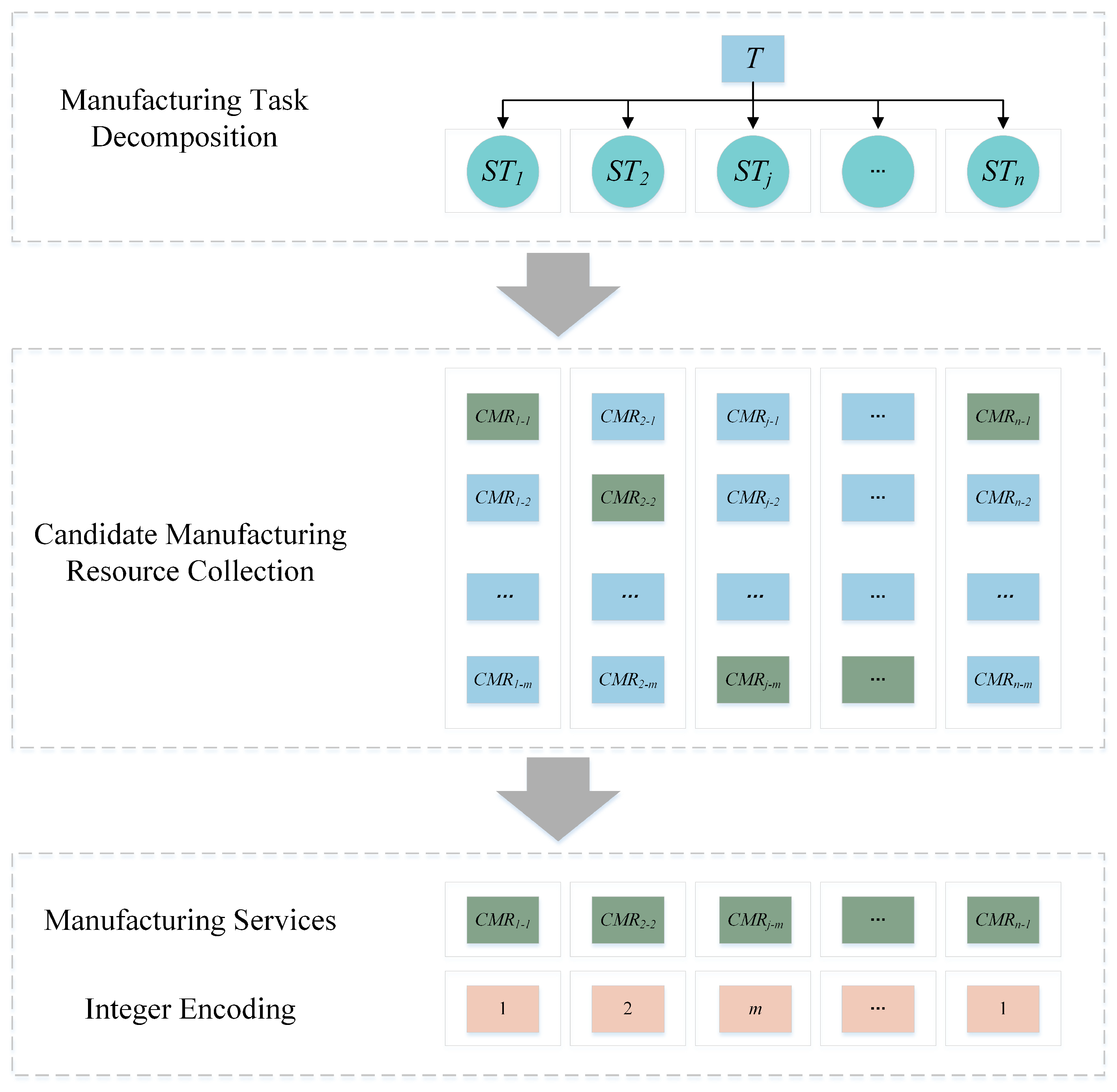
In the sewing machine cases manufacturing service composition optimization problem, sub-task ST is used as a path for manufacturing service composition optimization. The following mathematical models can be used to express this mapping relationship, as shown in Equations (29) and (30):
where the dimension of the search space Q is n × m, STn represents the nth subtask; CMRn-m represents the mth candidate service in the candidate manufacturing service set corresponding to the nth ST subtask; CMSP represents the pth scheme; and CMRp-i represents the CMR number in the candidate manufacturing service set selected by the ith subtask in the pth scheme.
The CMR is encoded using an integer encoding method, and its length is equal to the number of subtasks. Each hummingbird’s position vector represents a composition scheme, as shown in Figure 5. If a set of manufacturing service compositions is selected, specifically {CMR1-1, CMR2-2, CMR3-m, …, CMRn-1}, then the final hummingbird individual integer encoding corresponding to this service can be represented as {1, 2, m, …, 1}.

Figure 5.
Hummingbird individual position encoding scheme.
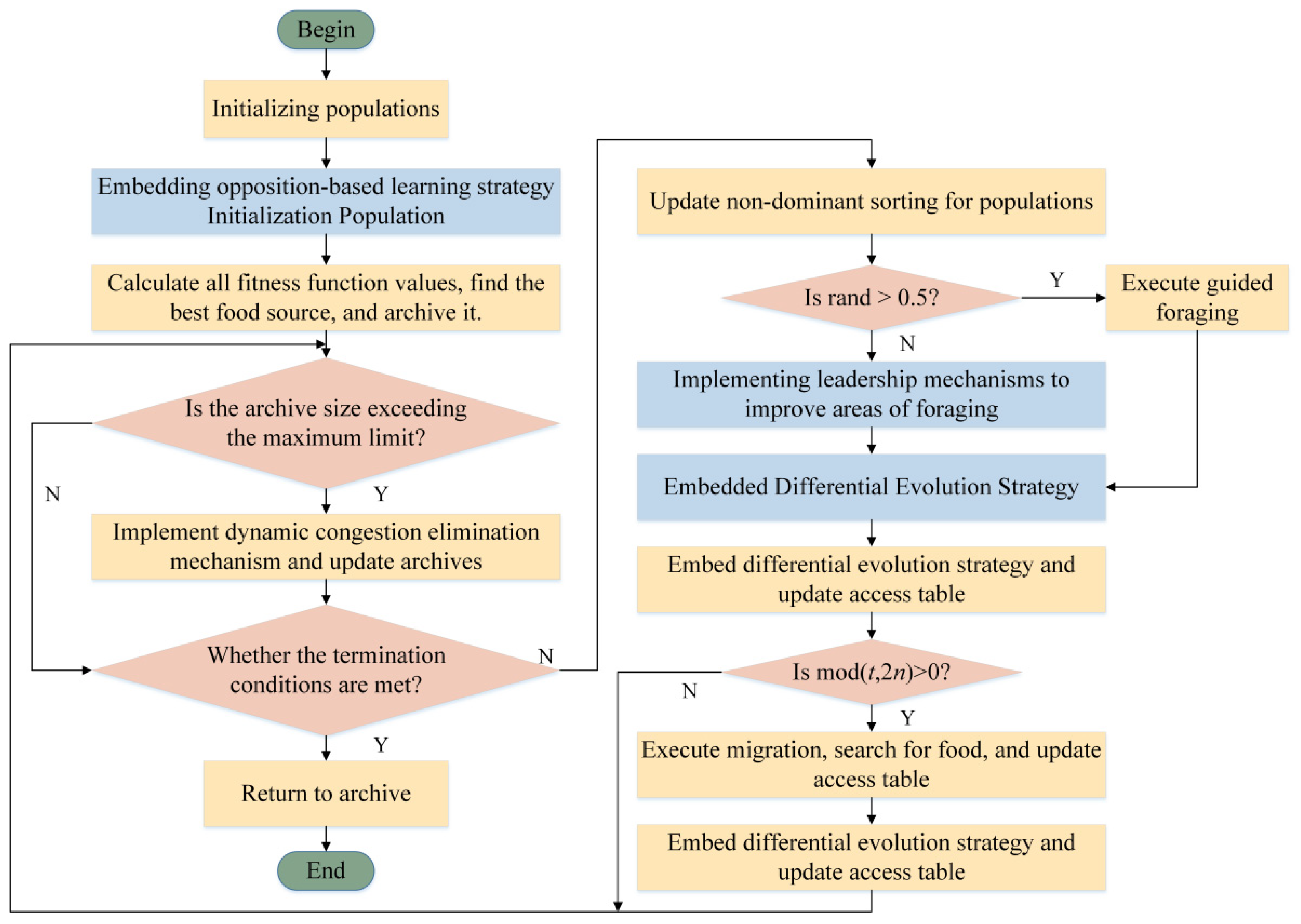
2.7. ORAHA_DE Algorithm Process Framework Diagram
Based on the above improvement process, the ORAHA_DE algorithm flowchart shown in Figure 6 can be obtained. The specific implementation steps are as follows:
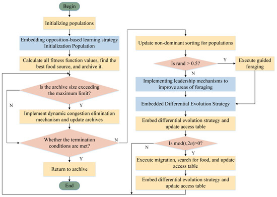
Figure 6.
ORAHA_DE algorithm flow framework diagram.
- Initialize parameters, including setting the hummingbird population size, iteration count, external archive size, search space dimension, and access table;
- The elite opposition-based learning strategy is integrated into the multi-objective hummingbird algorithm. By generating opposition solutions that are opposite to the current solution, the objective function values of all hummingbirds are evaluated, and the current solution is added to the external archive;
- Determine whether the number of solutions in the archive exceeds the maximum value. If it exceeds the maximum number of solutions, execute the dynamic congestion distance elimination strategy. If it does not exceed the maximum number of solutions, proceed to step 4;
- Determine whether the iteration termination condition has been met. If so, save the archive and terminate the algorithm. If not, perform a non-dominated sorting update on the population and proceed to step 5;
- Check if the rand value is greater than 0.5. If so, execute the guided foraging strategy. If not, select the leader improvement domain foraging operation using the roulette wheel selection strategy. Upon completion, update the access table;
- Execute the Lévy flight-enhanced differential evolution strategy, add the population to the archive, and synchronously update the dominance relationships;
- Determine whether mod (t, 2n) = 0 is true. If so, execute the migration foraging strategy and synchronously update the dominance relationship. If not, return to step 3 and re-enter the loop.
2.8. Algorithm Performance Indicators
When evaluating the performance of multi-objective optimization algorithms, comprehensive performance measurement methods are one type of indicator that can comprehensively consider the convergence and distribution of approximate solution sets. The most commonly used indicators include Generational Distance (GD) and Hypervolume (HV):
- GD [39] is used to measure the distance between the Pareto frontier found by the algorithm and the true Pareto frontier, as shown in Formula (31):
- 2.
- HV [40] is used to measure the hypervolume covered by the Pareto frontier, as shown in Equation (32):
3. Results
In order to verify the superiority and feasibility of the ORAHA_DE algorithm in solving the sewing machine cases manufacturing service composition optimization model, algorithm performance comparison and scale expansion examples were designed to verify the algorithm performance. The aforementioned operations were performed using MATLAB software (version R2024b), an Intel (R) Core (TM) i5-12400F processor (2.50 GHz), 16.0 GB of RAM, an NVIDIA GeForce GT1050Ti graphics card, a 1 TB HDD hard drive, and the Windows 11 Professional 24H2 operating system. In experiments calculating the maximum data volume, the computer configuration achieved a CPU peak of 67%, a GPU peak of 3.0 GB/4 GB, and memory of 7.9 GB/16 GB, with ample capacity remaining, indicating that the computer performance under this configuration is sufficient for this experiment.
3.1. Algorithm Performance Comparison
3.1.1. Benchmark Function Comparison
This paper introduces NSGA-II, NSGA-III, MODE, MOAHA, MOGWO, and ORAHA_DE algorithms for comparison. The initial conditions of various algorithms are set under the same experimental environment as shown in Table 1.

Table 1.
Parameter settings for various algorithms.
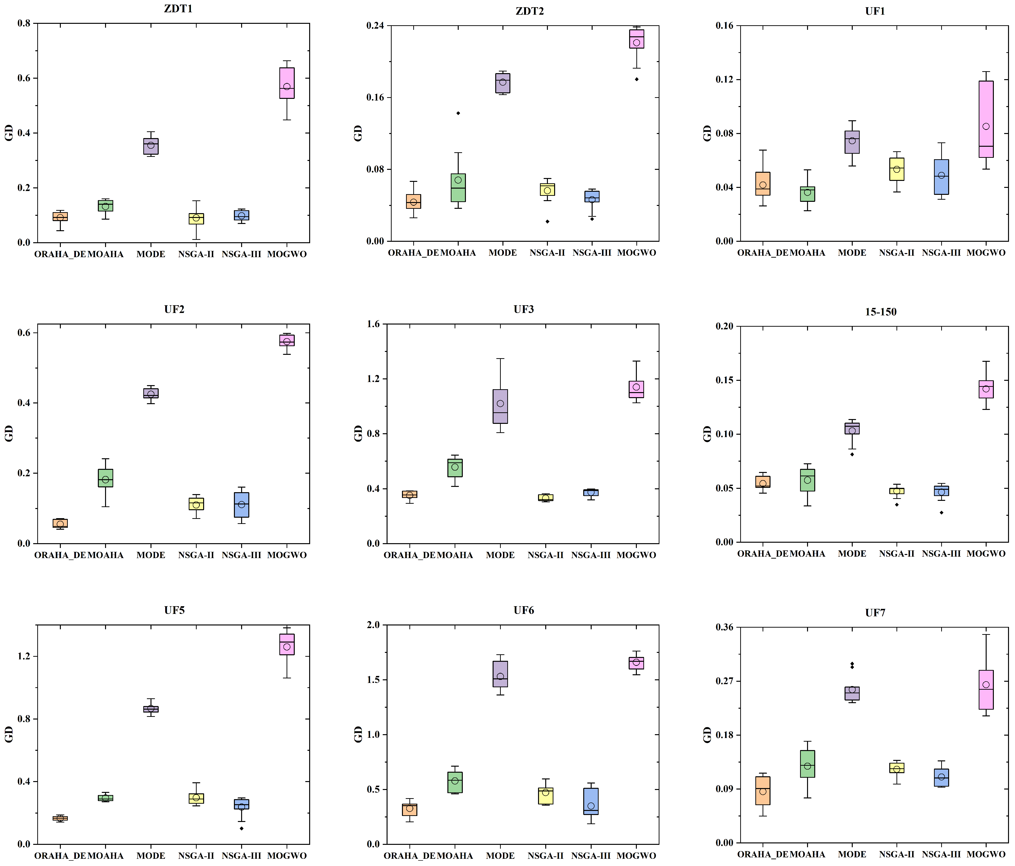
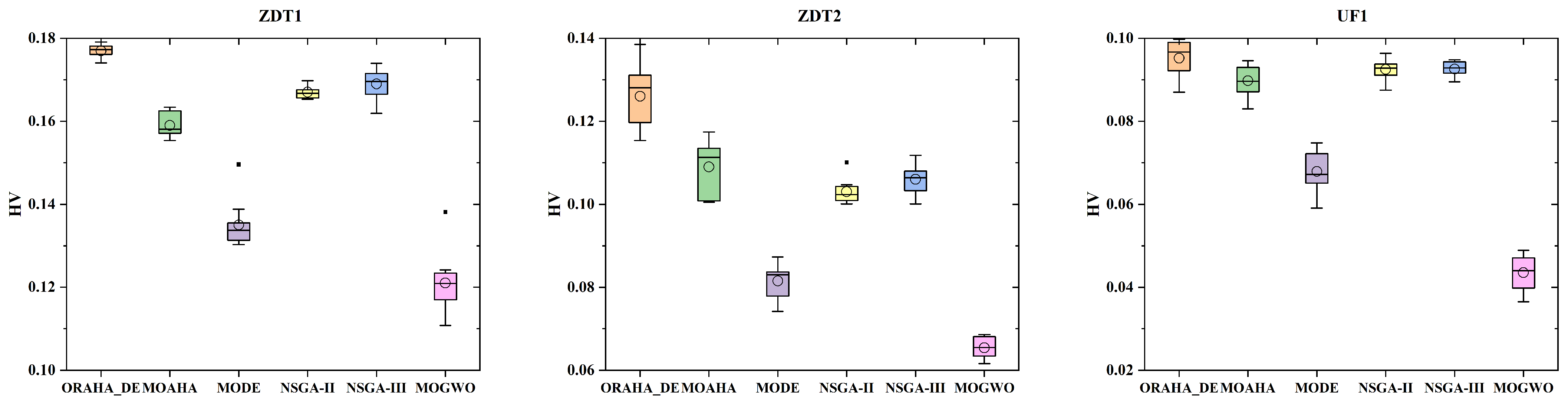
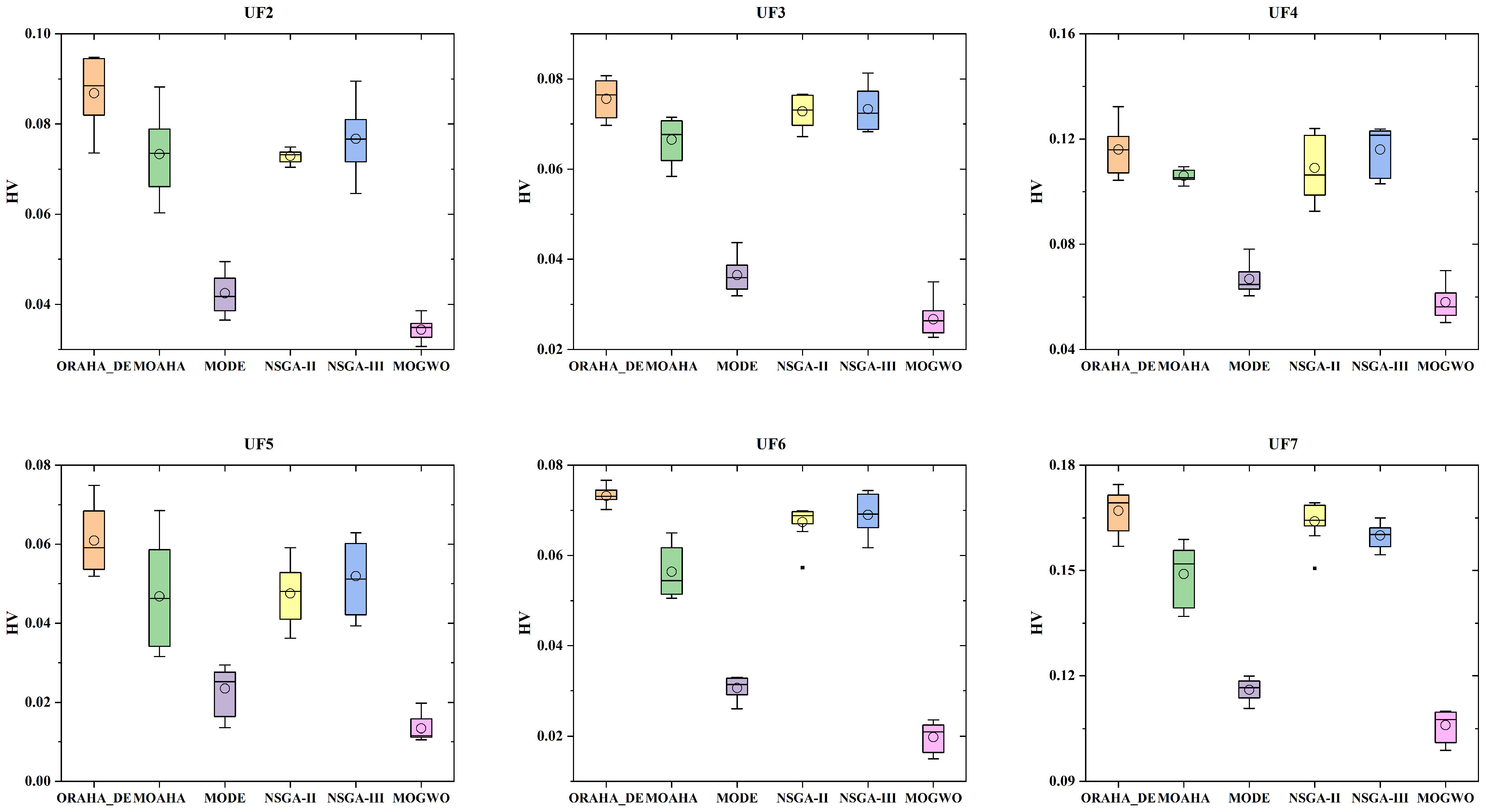
The ZDT1 and ZDT2 functions from the ZDT function set (Zitzler-Deb-Thiele Test Function Set) and the UF1-7 functions from the UF function set (Unconstrained Function Set) were introduced as test functions to evaluate the GD and HV values. The calculation results are shown in Table 2 and Table 3. The (Mean/Std) column indicates the mean and standard deviation. The optimal results among all algorithms are bolded in Table 2 and Table 3. For GD value results, a smaller Mean value and a smaller Std value are better; for HV value results, a larger Mean value and a smaller Std value are better. As shown in Table 2, the ORAHA_DE algorithm has the best Mean value for the GD indicator in all test functions except UF1 and UF4. The MOAHA only has the best Mean value for the UF1 scale problem, and the NSGA-III algorithm has the best Mean value for the UF4 scale problem. As shown in Table 3, the ORAHA_DE algorithm has the best Mean value for the HV indicator in all test functions. The experimental results show that among the selected benchmark functions, the ORAHA_DE algorithm has obvious advantages over the other algorithms in terms of the GD indicator and HV indicator.
Table 2.
GD indicator results.
Table 3.
HV indicator results.
To more intuitively demonstrate the performance differences in all algorithms under different test functions, box plots comparing the GD and HV metrics of different algorithms across nine test functions are presented, as shown in Figure 7 and Figure 8. In the box plots, circles represent the mean value, and the black dots represent the errors. As shown in Figure 7, in most cases, the GD value box plot corresponding to the ORAHA_DE algorithm is at the lowest position, indicating that this algorithm performs better than other algorithms. Additionally, the narrow box plot suggests that the ORAHA_DE algorithm has better stability. In Figure 8, it can be seen that in most cases, the box plot of the HV values corresponding to the ORAHA_DE algorithm is at a high position, indicating that the ORAHA_DE algorithm covers a larger Pareto frontier hypervolume with higher quality. Additionally, the narrow box plot indicates that the ORAHA_DE algorithm has better stability.
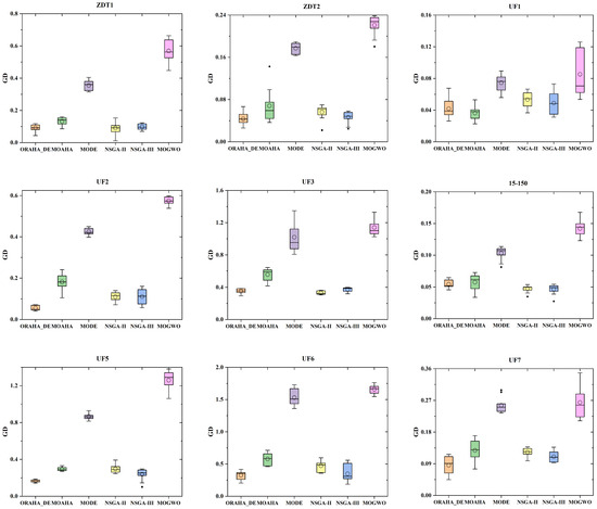
Figure 7.
GD indicator box plot diagram.
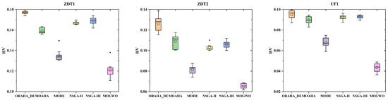
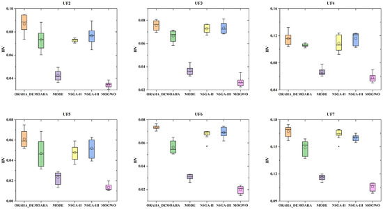
Figure 8.
HV indicator box plot diagram.
3.1.2. Wilcoxon Signed-Rank Test
In order to better evaluate the significant differences between the ORAHA_DE algorithm and the other five algorithms in terms of GD and HV indicators, this paper conducted a Wilcoxon signed-rank test. The results of comparing the ORAHA_DE algorithm with the other five algorithms are shown in Table 4 and Table 5, where the symbols “+”, “−”, and “≈” are used to indicate whether the ORAHA_DE algorithm is superior, inferior, or similar to the other algorithms in terms of GD and HV indicators, respectively.
Table 4.
Results of the Wilcoxon signed-rank test for the GD indicator.
Table 5.
Results of the Wilcoxon signed-rank test for the HV indicator.
As shown in Table 4, the ORAHA_DE algorithm outperforms the MOAHA in almost all test functions in terms of GD indicators, outperforms the MODE algorithm and MOGWO algorithm in nine test functions, and outperforms the NSGA-II and NSGA-III algorithms in five test functions. Furthermore, the ORAHA_DE algorithm has no disadvantage in terms of GD values compared to all comparison algorithms.
As shown in Table 5, the ORAHA_DE algorithm outperformed the MODE and MOGWO algorithms in terms of the HV indicator for almost all test functions; it outperformed the MOAHA, NSGA-II, and NSGA-III algorithms in three test functions, and performed similarly to these three algorithms in the remaining six test functions. Furthermore, the ORAHA_DE algorithm did not have a disadvantage in terms of the HV value compared to all the other algorithms.
3.1.3. Friedman Test
The Friedman test was performed using the above statistical data to determine the rankings of different algorithms in terms of GD and HV indicators. The results of the Friedman test for GD and HV indicators are shown in Table 6. The p-value of the GD indicator is 5.11 × 10⁻⁵ < 0.05, and the p-value of the HV indicator is 2.20 × 10⁻¹⁶ < 0.05, which indicates that there are significant differences between the compared algorithms. In addition, the ORAHA_DE algorithm ranked first in both the GD indicator and the HV indicator, indicating that this algorithm has a comparative advantage over other algorithms in solving this problem.
Table 6.
Friedman’s test for GD indicator and HV indicator.
3.2. Case Studies
In order to further verify the applicability of the ORAHA_DE algorithm in the service composition optimization problem of sewing machine cases, this paper set up experiments based on a self-built database and simulated data derived from real data. Some of the data used in the experiment are shown in Table 7. In order to ensure generality, the attribute value parameters of the candidate service normalization were randomly initialized within a specific range, as shown in Table 8.
Table 7.
Some of the data used in the experiment.
Table 8.
Range of values for attribute indicators.
When the service requester sends a manufacturing request to the collaborative manufacturing platform, the platform breaks down the part manufacturing task into a bunch of subtasks based on the manufacturing process flow for the part. The sewing machine cases manufacturing task can be broken down into 10 processes. In this study, assuming that each process in the sewing machine cases manufacturing corresponds to 50 candidate service sets, the sewing machine cases manufacturing task instance can be represented as (10–50). In order to further verify the applicability of the ORAHA_DE algorithm in solving the sewing machine cases manufacturing service composition optimization model, this paper extends the sewing machine cases manufacturing task instance to nine sewing machine base manufacturing tasks of different scales, represented as {(10–50), (10–100), (10–150), (15–50), (15–100), (15–150), (20–50), (20–100), (20–150)}. Each of the six algorithms is then run independently 20 times.
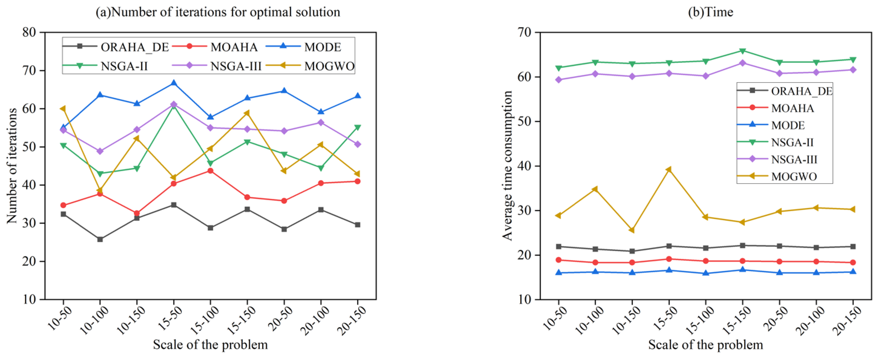
3.2.1. Comparison of Convergence Speed and Time
By comparing the optimal average number of iterations and average time consumption of six algorithms in solving nine different-scale composition optimization problems, the results are shown in Figure 9. Figure 9a shows the optimal average iteration counts of the six algorithms under conditions of a population size of 100 and 300 iterations. The ORAHA_DE algorithm has optimal solution average iteration counts concentrated around 30 iterations across the nine problem scales, while the MOAHA’s iteration counts are concentrated around 40 iterations. This is because the ORAHA_DE algorithm incorporates a Lévy flight-enhanced differential evolution strategy, reducing the number of iterations required to find the optimal solution. However, the optimal solution iteration counts for the other four algorithms are concentrated between 45 and 75 iterations, all higher than the optimal iteration count of the ORAHA_DE algorithm. Figure 9b compares the average time consumption of the six algorithms in solving nine different-scale composition optimization problems. It can be seen that although the time consumption of the ORAHA_DE algorithm in obtaining the optimal solution is slightly higher than that of the MODE algorithm and MOAHA, the difference is not significant and is still within an acceptable range. This is due to the three improved strategies embedded in the ORAHA_DE algorithm. The ORAHA_DE algorithm requires less time than the MOGWO algorithm; the NSGA-II and NSGA-III algorithms require significantly more time than other algorithms, nearly three times the time consumed by the ORAHA_DE algorithm.
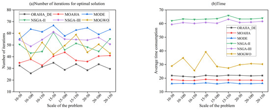
Figure 9.
Fitness and average time consumption of different algorithms for solving problems.
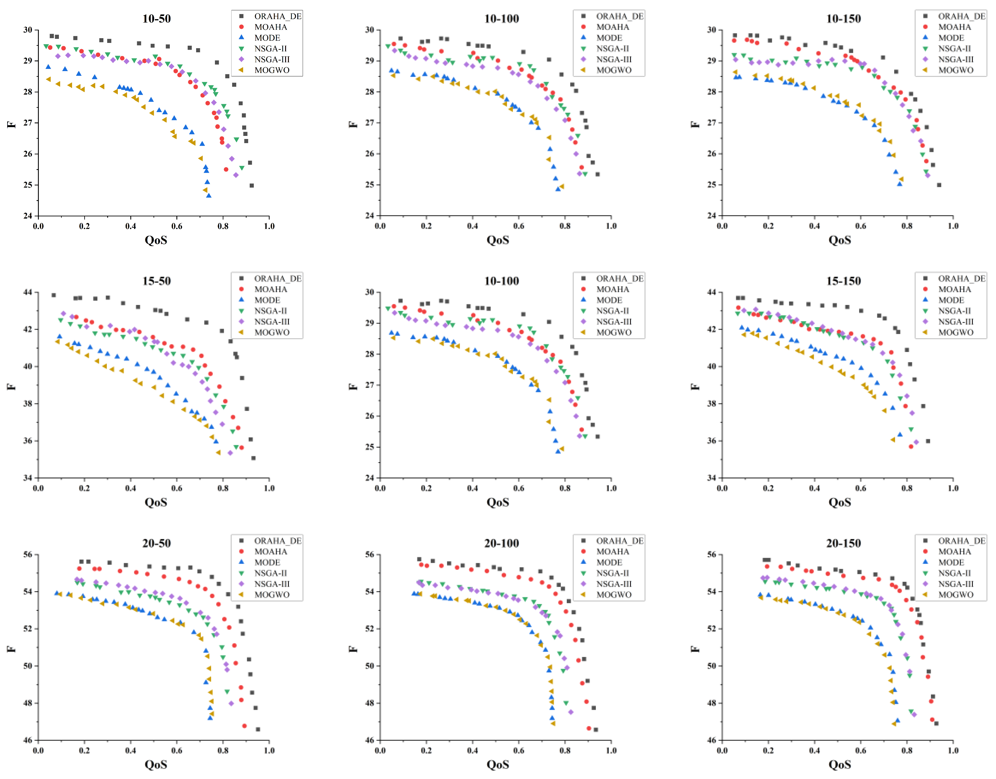
3.2.2. Optimal Solution Distribution
Through instance verification using self-built database data, we obtained the distribution of optimal solutions for six algorithms in solving nine different-scale sewing machine cases composition optimization problems, as shown in Figure 10. Among them, most of the gray data points solved by the ORAHA_DE algorithm are located in the upper right outer layer area. In addition, as the scale of the problem expands, the data points solved by the ORAHA_DE algorithm are always located on the outer edge of the two-dimensional graph, which shows that the ORAHA_DE algorithm is not only applicable to small-scale service composition optimization problems but also to large-scale service composition optimization problems.
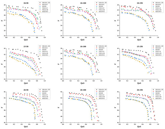
Figure 10.
Distribution of optimal solutions for nine different composition optimization problems.
Through empirical verification, we obtained the optimal solution composition for the service composition optimization problem of nine sewing machine cases, as shown in Table 9.
Table 9.
Optimal manufacturing service composition at different scales.
4. Discussion
This paper takes sewing machine cases as the research object. Through field research in enterprises, the service indicators valued by manufacturing service demanders and manufacturing resource service providers are collected and sorted. Based on the actual manufacturing situation reflected by manufacturing enterprises, subtle adjustments are made to establish a service composition optimization model that considers both QoS indicators and flexibility indicators. The ORAHA_DE algorithm is used to solve the mathematical model of sewing machine cases manufacturing service composition optimization. Therefore, in order to prove the applicability and effectiveness of the ORAHA_DE algorithm, this paper verifies the effectiveness of this method from two aspects: algorithm performance comparison and scale instance verification.
This paper mainly focuses on verification using medium- and small-scale examples, verifying that the ORAHA_DE algorithm can maintain good optimization capabilities even when the number of processes and the number of service candidate sets increase. The running time and the average number of iterations required to obtain the optimal solution fluctuate within a reasonable range, proving that the algorithm has the potential to be extended to larger-scale sewing machine cases manufacturing tasks.
However, this study still has some limitations. In terms of manufacturing, the number of steps in the manufacturing process of sewing machine cases may exceed the maximum number of 20 steps experimented in this study. A larger number of steps also means more manufacturing resource service sets and more manufacturers participating in the process, which also means that the manufacturing service composition is more complex. In addition, in terms of the service evaluation indicator system, the evaluation indicators involved in this paper also have limitations. In the actual production process, there will be more service evaluation indicators involved, and they will also be complex and variable. These uncertainties will also affect the experimental results. In future research, the number of sewing machine cases production processes can be increased, for example, to 30 or even 40 processes. At the same time, the number of manufacturing resource service sets can also be increased, for example, to 200 or even 300 manufacturing resource service sets. In future experiments, uncertain factors in the service evaluation indicators can also be increased, such as enterprise manufacturing qualification rates, enterprise geographical locations, and manufacturing transportation costs.
5. Conclusions
This paper proposes a method to address the issue of low collaborative efficiency in subcontracted processing at the part level in the manufacturing of sewing machine cases under a network-based collaborative manufacturing model. This approach enhances production efficiency, reduces production time, and lowers production costs. By applying the ORAHA_DE algorithm to solve the service combination optimization model for sewing machine cases manufacturing, experimental validation yields the following conclusions:
- Compared with the other five multi-objective optimization algorithms, the GD indicator of the ORAHA_DE algorithm had the smallest value in seven of the nine different test functions, with a minimum value of 4.35 × 10⁻², indicating that the Pareto frontier found by the ORAHA_DE algorithm was closer to the true Pareto frontier and significantly better than the other five algorithms. The HV indicator had the maximum value in all nine test functions, with a maximum value of 1.77 × 10⁻¹, indicating that the Pareto frontier found by the ORAHA_DE algorithm was of higher quality. The Wilcoxon signed-rank test shows that the GD and HV values of the ORAHA_DE algorithm are significantly better than those of other algorithms in most test functions. The Friedman test shows that the ORAHA_DE algorithm ranks first in both the GD and HV indicators, and the p-value is much less than 0.05, indicating that there is a significant difference between the ORAHA_DE algorithm and the other five algorithms, and that its overall performance is the best. Additionally, Figure 6 and Figure 7 demonstrate that the ORAHA_DE algorithm exhibits relatively higher stability across different test functions.
- When solving nine different-scale sewing machine cases composition optimization problems, the average number of iterations for the optimal solution of the ORAHA_DE algorithm was around 30, while that of the MOAHA was around 40. However, the number of iterations for the optimal solution of the other four algorithms ranged from 45 to 75, which was higher than that of the ORAHA_DE algorithm. By testing the time consumed in solving nine different-scale sewing machine cases manufacturing composition optimization problems, we can conclude that the ORAHA_DE algorithm takes slightly longer than the MODE algorithm and the MOAHA to find the optimal solution, but much less time than the NSGA-II and NSGA-III algorithms. The average time taken by the ORAHA_DE algorithm to solve nine different-sized sewing machine cases manufacturing problems is between 20.88 and 22.15 s. As the dataset size increases from (10–50) to (20–150), the ORAHA_DE algorithm achieves the optimal solution with an average of 30 ± 5 iterations and an average solution time of 21.5 ± 0.65 s across different problem scales. Compared to other algorithms, it consistently demonstrates a certain advantage, indicating that this algorithm maintains its performance even as the number of processes increases, the number of candidate services grows, and when the dataset is expanded, the quality of the solution set remains virtually unaffected, suggesting that the performance of this method is not significantly impacted by dataset expansion.
- By comparing the optimal solutions of different algorithms in service composition optimization problems, it can be concluded that the optimal solution obtained by the ORAHA_DE algorithm is superior to other algorithms. When the QoS indicator is high, there is also a high flexibility indicator. In the composition optimization problems of sewing machine cases with 10, 15, and 20 processes, the optimal solution values of the QoS indicator are concentrated between (0.86–0.90), (0.83–0.91), and (0.87–0.92), respectively, while the optimal solution values for the flexibility indicator are concentrated between (28.23–29.07), (41.35–42.83), and (53.86–55.43), respectively.
Author Contributions
Conceptualization, G.S. and S.L.; methodology, G.S. and K.S.; software, L.Z. and K.S.; validation, Z.G. and K.S.; formal analysis, G.S.; investigation, J.Z.; resources, G.S. and Z.G.; data curation, K.S.; writing—original draft preparation, G.S.; writing—review and editing, G.S. and S.L.; visualization, G.S.; supervision, L.Z.; project administration, G.S. and J.Z.; funding acquisition, S.L. All authors have read and agreed to the published version of the manuscript.
Funding
This research was funded by the National Key Research and Development Program of China (Program No. 2023YFB3308800).
Data Availability Statement
The data used in this study comes from the core business databases of real companies and involves sensitive commercial information that cannot be made public. If there is a reasonable academic need, researchers can apply to the authors to use the data.
Conflicts of Interest
Authors K.S. and L.Z. are employed by Xi’an Aerospace-Huayang Mechanical & Electrical Equipment Co., Ltd. The remaining authors declare that this research was conducted in the absence of any commercial or financial relationships that could be construed as a potential conflict of interest.
References
- Camarinha-Matos, L. Collaborative networked organizations: Status and trends in manufacturing. Annu. Rev. Control 2009, 33, 199–208. [Google Scholar] [CrossRef]
- Zhang, W.; Zhang, S.; Chen, G. Combining social network and collaborative filtering for personalised manufacturing service recommendation. Int. J. Prod. Res. 2013, 51, 6702–6719. [Google Scholar] [CrossRef]
- Cheng, Y.; Bi, L.; Tao, F. Hypernetwork-based manufacturing service scheduling for distributed and collaborative manufacturing operations towards smart manufacturing. J. Intell. Manuf. 2020, 31, 1707–1720. [Google Scholar] [CrossRef]
- Leng, J.; Jiang, P. Evaluation across and within collaborative manufacturing networks: A comparison of manufacturers’ interactions and attributes. Int. J. Prod. Res. 2018, 56, 5131–5146. [Google Scholar] [CrossRef]
- Zhang, X.; Ming, X.; Bao, Y. Networking-enabled product service system (N-PSS) in collaborative manufacturing platform for mass personalization model. Comput. Ind. Eng. 2022, 163, 107805. [Google Scholar] [CrossRef]
- Tao, F.; Zhao, D.; Yefa, H. Correlation-aware resource service composition and optimal-selection in manufacturing grid. Eur. J. Oper. Res. 2010, 201, 129–143. [Google Scholar] [CrossRef]
- Liu, S.; Zhang, Z.; Jiang, X. An optimal selection method of cloud manufacturing resource for guide roller based on combination algorithm. J. Imaging Sci. Technol. 2024, 68, 1. [Google Scholar] [CrossRef]
- Fazeli, M.; Farjami, Y.; Nickray, M. An ensemble optimisation approach to service composition in cloud manufacturing. Int. J. Comput. Integr. Manuf. 2019, 32, 83–91. [Google Scholar] [CrossRef]
- Hu, Q.; Qi, H.; Jia, Y. A two-phase method to optimize service composition in cloud manufacturing. Computing 2024, 106, 2261–2291. [Google Scholar] [CrossRef]
- Cai, A.; Guo, Z.; Guo, S. Optimization strategy of knowledge service composition in cloud manufacturing environment. Comput. Integr. Manuf. Syst. 2019, 25, 421–430. [Google Scholar] [CrossRef]
- Song, C.; Zheng, H.; Han, G. Cloud edge collaborative service composition optimization for intelligent manufacturing. IEEE Trans. Ind. Inform. 2022, 19, 6849–6858. [Google Scholar] [CrossRef]
- Rodriguez-Mier, P.; Mucientes, M.; Lama, M. Hybrid optimization algorithm for large-scale QoS-aware service composition. IEEE Trans. Serv. Comput. 2015, 10, 547–559. [Google Scholar] [CrossRef]
- Sodhro, A.H.; Malokani, A.S.; Sodhro, G.H.; Muzammall, M.; Zongwei, L. An adaptive QoS computation for medical data processing in intelligent healthcare applications. Neural Comput. Appl. 2020, 32, 723–734. [Google Scholar] [CrossRef]
- Badawy, M.M.; Ali, Z.H.; Ali, H.A. QoS provisioning framework for service-oriented internet of things (IoT). Clust. Comput. 2020, 23, 575–591. [Google Scholar] [CrossRef]
- Sun, W.; Wang, Z.; Zhang, G. A QoS-guaranteed intelligent routing mechanism in software-defined networks. Comput. Netw. 2021, 185, 107709. [Google Scholar] [CrossRef]
- Yu, Y.; Li, S.; Ma, J. Time-aware cloud manufacturing service selection using unknown QoS prediction and uncertain user preferences. Concurr. Eng. 2021, 29, 370–385. [Google Scholar] [CrossRef]
- Ma, H.; Zhang, Y.; Sun, S. A comprehensive survey on NSGA-II for multi-objective optimization and applications. Artif. Intell. Rev. 2023, 56, 15217–15270. [Google Scholar] [CrossRef]
- Ranjan, S.; Gupta, R.; Nanda, S. Threshold based constrained θ-NSGA-III algorithm to solve many-objective optimization problems. Inf. Sci. 2025, 697, 121751. [Google Scholar] [CrossRef]
- Shu, X.; Liu, Y.; Liu, J. Multi-objective particle swarm optimization with dynamic population size. J. Comput. Des. Eng. 2023, 10, 446–467. [Google Scholar] [CrossRef]
- Makhadmeh, S.; Alomari, O.; Mirjalili, S. Recent advances in multi-objective grey wolf optimizer, its versions and applications. Neural Comput. Appl. 2022, 34, 19723–19749. [Google Scholar] [CrossRef]
- Khodadadi, N.; Mirjalili, S.; Zhao, W. Multi-Objective Artificial Hummingbird Algorithm//Advances in Swarm Intelligence: Variations and Adaptations for Optimization Problems; Springer International Publishing: Cham, Switzerland, 2022; pp. 407–419. [Google Scholar] [CrossRef]
- Mirjalili, S.; Mirjalili, S.; Saremi, S. Grasshopper optimization algorithm for multi-objective optimization problems. Appl. Intell. 2018, 48, 805–820. [Google Scholar] [CrossRef]
- Basu, M. Economic environmental dispatch using multi-objective differential evolution. Appl. Soft Comput. 2011, 11, 2845–2853. [Google Scholar] [CrossRef]
- Gao, Z.; Liu, S.; Qian, S.; Zhu, L.; Shi, G.; Zhao, J. A Resource Composition Optimization Algorithm Based on Improved Polar Bear Optimization Algorithm for Manufacturing Wallboard for Coating Machine. Coatings 2025, 15, 418. [Google Scholar] [CrossRef]
- Li, F.; Zhang, L.; Liu, Y. QoS-aware service composition in cloud manufacturing: A Gale–Shapley algorithm-based approach. IEEE Trans. Syst. Man Cybern. Syst. 2018, 50, 2386–2397. [Google Scholar] [CrossRef]
- Zhang, Y.; Cui, G.; Wang, Y. An optimization algorithm for service composition based on an improved FOA. Tsinghua Sci. Technol. 2015, 20, 90–99. [Google Scholar] [CrossRef]
- Zhang, C.; Ning, J.; Wu, J. A multi-objective optimization method for service composition problem with sharing property. Swarm Evol. Comput. 2019, 49, 266–276. [Google Scholar] [CrossRef]
- Yang, Y.; Yang, B.; Wang, S. A dynamic ant-colony genetic algorithm for cloud service composition optimization. Int. J. Adv. Manuf. Technol. 2019, 102, 355–368. [Google Scholar] [CrossRef]
- Seghir, F. Fdmoabc: Fuzzy discrete multi-objective artificial bee colony approach for solving the non-deterministic QoS-driven web service composition problem. Expert Syst. Appl. 2021, 167, 114413. [Google Scholar] [CrossRef]
- Zhu, L.; Jiang, Z.; Shi, J.; Jin, C. An overview of turn-milling technology. Int. J. Adv. Manuf. Technol. 2015, 81, 493–505. [Google Scholar] [CrossRef]
- Ivanov, V.; Evtuhov, A.; Dehtiarov, I.; Trojanowska, J. Fundamentals of Manufacturing Engineering Using Digital Visualization; Springer Nature: Berlin, Germany, 2025. [Google Scholar] [CrossRef]
- Yang, Y.; Yang, B.; Wang, S.; Liu, W.; Jin, T. An improved grey wolf optimizer algorithm for energy-aware service composition in cloud manufacturing. Int. J. Adv. Manuf. Technol. 2019, 105, 3079–3091. [Google Scholar] [CrossRef]
- Zhao, W.; Zhang, Z.; Mirjalili, S.; Wang, L.; Khodadadi, N.; Mirjalili, S.M. An effective multi-objective artificial hummingbird algorithm with dynamic elimination-based crowding distance for solving engineering design problems. Comput. Methods Appl. Mech. Eng. 2022, 398, 115223. [Google Scholar] [CrossRef]
- Zhao, W.; Wang, L.; Mirjalili, S. Artificial hummingbird algorithm: A new bio-inspired optimizer with its engineering applications. Comput. Methods Appl. Mech. Eng. 2022, 388, 114194. [Google Scholar] [CrossRef]
- Mahdavi, S.; Rahnamayan, S.; Deb, K. Opposition based learning: A literature review. Swarm Evol. Comput. 2018, 39, 1–23. [Google Scholar] [CrossRef]
- Mirjalili, S.; Saremi, S.; Mirjalili, S.; Coelho, L.d.S. Multi-objective grey wolf optimizer: A novel algorithm for multi-criterion optimization. Expert Syst. Appl. 2016, 47, 106–119. [Google Scholar] [CrossRef]
- Storn, R.; Price, K. Differential evolution-a simple and efficient heuristic for global optimization over continuous spaces. J. Glob. Optim. 1997, 11, 341. [Google Scholar] [CrossRef]
- Wang, Y.; Ran, S.; Wang, G. Role-oriented binary grey wolf optimizer using foraging-following and lévy flight for feature selection. Appl. Math. Model. 2024, 126, 310–326. [Google Scholar] [CrossRef]
- Gao, Y.; Yang, B.; Wang, S.; Zhang, Z.; Tang, X. Bi-objective service composition and optimal selection for cloud manufacturing with QoS and robustness criteria. Appl. Soft Comput. 2022, 128, 109530. [Google Scholar] [CrossRef]
- Zhang, Q.; Li, S.; Pu, R.; Zhou, P.; Chen, G.; Li, K.; Lv, D. An adaptive robust service composition and optimal selection method for cloud manufacturing based on the enhanced multi-objective artificial hummingbird algorithm. Expert Syst. Appl. 2024, 244, 122823. [Google Scholar] [CrossRef]

Disclaimer/Publisher’s Note: The statements, opinions and data contained in all publications are solely those of the individual author(s) and contributor(s) and not of MDPI and/or the editor(s). MDPI and/or the editor(s) disclaim responsibility for any injury to people or property resulting from any ideas, methods, instructions or products referred to in the content. |
© 2025 by the authors. Licensee MDPI, Basel, Switzerland. This article is an open access article distributed under the terms and conditions of the Creative Commons Attribution (CC BY) license (https://creativecommons.org/licenses/by/4.0/).