Decentralized Energy Management for Microgrids Using Multilayer Perceptron Neural Networks and Modified Cheetah Optimizer

Abstract

This paper presents a decentralized energy management system (EMS) based on Multilayer Perceptron Artificial Neural Networks (MLP-ANNs) and a Modified Cheetah Optimizer (MCO) to account for uncertainty in renewable generation and load demand. The proposed framework applies an MLP-ANN with Levenberg–Marquardt (LM) training for high-precision forecasts of photovoltaic/wind generation, ambient temperature, and load demand, greatly outperforming traditional statistical methods (e.g., time-series analysis) and resilient backpropagation (RP) in precision. The new MCO algorithm eliminates local trapping and premature convergence issues in classical optimization methods like Particle Swarm Optimization (PSO) and Genetic Algorithms (GAs). Simulations on a test microgrid verily demonstrate the advantages of the framework, achieving a 26.8% cost-of-operation reduction against rule-based EMSs and classical PSO/GA, and a 15% improvement in forecast accuracy using an LM-trained MLP-ANN. Moreover, demand response programs embodied in the system reduce peak loads by 7.5% further enhancing grid stability. The MLP-ANN forecasting–MCO optimization duet is an effective and cost-competitive decentralized microgrid management solution under uncertainty.

1. Introduction

The global energy market is shifting toward renewable energy sources (RESs) as a response to climate change and shrinking stocks of fossil fuels [1]. The shift is made easier through effective policy frameworks such as the Paris Agreement and local policies like the European Green Deal [2], which establish challenging renewable penetration targets. Microgrids are an effective solution for achieving such targets, due to their decentralized control of energy, which can enhance grid robustness and reduce transmission losses [3]. The natural fluctuation in photovoltaic (PV) and wind turbine (WT) energy, as well as non-stationary loads, is a primary challenge for energy management systems (EMSs) [4]. Real-time decision-making in dynamic situations, in which classical prediction and optimization methods are not always effective [5], makes things even more difficult.

Current advancements in machine learning (ML) offer promise in overcoming such challenges. The multilayer perceptron artificial neural networks (MLP-ANNs), when trained on the Levenberg–Marquardt (LM) algorithm, in general, are seen to be quite effective in predicting PV and WT generation, achieving as low as 8.22% in solar irradiance’s mean absolute percentage errors [6]. The LM algorithm is preferred to others like resilient backpropagation (RP) due to high levels of accuracy as well as rapid convergence [6,7,8]. Support Vector Regression (SVR) models also are seen to be effective, employing previous energy production and weather data to optimize accuracy in forecasts as well as optimize resource allocation [9]. Hybrid ensemble approaches, such as bidirectional long-term memory combined with gradient boosting decision trees and random forests, have further reduced RMSE by 10% in wind power forecasting [10]. Similarly, extreme gradient boosting (XGBoost) has outperformed SVR and Long Short-Term Memory (LSTM) in short-term solar generation predictions [11]. Notably, new architectures like Temporal Fusion Transformers (TFTs) and hybrid models that merge recurrent neural networks with feature selection techniques [12,13] have significantly improved prediction accuracy, demonstrating a reduction in root mean square error (RMSE) by about 10–15% when compared to conventional statistical approaches [4]. In addition, approaches that involve wavelet transformations in conjunction with machine learning platforms show promise in identifying non-linear periodic patterns in renewable energy data [14]. However, issues remain in terms of incorporating high-resolution environmental data and model evaluation across different microgrid setups [15].

In optimization, traditional methods, such as particle swarm optimization (PSO) and genetic algorithms (GAs), are widely utilized for task scheduling in microgrids [3,16]. However, these methods often face premature convergence and computational inefficiency issues, especially under high-dimensional real-time scenarios [17,18]. More recent algorithms, such as the Multi-Objective War Strategy Optimization (MOWSO) [19] and the Enhanced Sparrow Search Algorithm (ESSA) [20], have shown significant improvements in the exploration–exploitation trade-off, achieving operational cost reductions of up to 18% while addressing carbon emission issues at the same time [19]. In this direction, several hybrid optimization approaches have recently appeared that combine PSO with the most advanced techniques, such as primal–dual interior point methods and multi-agent system-based frameworks [21,22]. Such hybrid models aim at providing even better performances in microgrid operation by properly exploiting the flexibility of PSO and the accuracy of more deterministic methods. It is such hybridization that has been able to address the concerns of system efficiency, power quality, and fuel consumption—issues that are of prime importance for real-world optimization of microgrid operation. Moreover, several advanced strategies have recently been proposed to mitigate issues related to energy management within microgrids. Within this context, the two-layer energy management system in [23] efficiently performed the optimization process of matching between batteries and fuel costs, with the help of goal programming techniques, proving that by increasing battery lifetimes, there would be a chance to reduce the total operating costs. Other metaheuristics, such as memory-based genetic algorithms [24] and grey wolf optimization [25], have also been applied with considerable success to optimize power distribution, reduce costs, and handle renewable variability. Advanced particle swarm optimization methods [26] have also shown potential in providing 24 h forecasts for load and renewable energy variations, thus ensuring better system adaptability. Hybrid approaches have also significantly enhanced energy management strategies. Fuzzy logic hybridized with grey wolf optimization has efficiently implemented operational cost minimization and fossil fuel emissions by optimally utilizing batteries and minimizing the dependency on conventional energy [27]. Chaotic and fuzzy self-adaptive particle swarm algorithms have also shown their effectiveness in the microgrid to minimize emissions and reduce costs in multi-objective optimization challenges [28]. Stand-alone microgrids have already adopted optimization techniques such as the application of a genetic algorithm in the optimal placement of renewable resources and storage devices. Such optimization techniques, by considering environmental variables such as wind and solar irradiance, optimized lifecycle costs while assuring efficient energy use [29]. Despite this, their scalability to larger microgrids of well over 100 nodes remains an important challenge [20].

The integration of demand response (DR) programs adds a new dimension to complexity in the management of microgrids. Recent studies show that dynamic pricing strategies, including critical peak pricing (CPP), can yield cost savings of 15.4% through price-sensitive demand response when combined with advanced optimization techniques like Greedy Rat Swarm Optimization [30]. Similarly, price structures responsive to classes, identified by Stackelberg game models, have proved effective in reducing peak–valley differentials while simultaneously improving participant utility [31]. Additionally, Thornburg et al. [32] ratified the benefits of demand-shifting and peak-shaving policies in isolated systems with high levels of renewable energy integration, thus staunching system reliability under generation volatilities. For hybrid AC/DC microgrids, incentivized DR programs, converged across various systems, have proved effective in optimizing energy scheduling and reducing operational costs through flexible resource optimization [33]. Industrial environments have proved potential, where smart DR programs considering photovoltaic (PV) uncertainty and battery cycling costs can result in lowered manufacturing costs while simultaneously reducing grid strain [34]. However, systematic analyses documented by Bakhtiari et al. [35] indicate that these strategies need to traverse three necessary dimensions: (1) economic effectiveness through mechanisms such as power capacity-based dynamic pricing (PCDP) [36], (2) technical constraints experienced in high-renewable environments [37], and (3) equity concerns relating to energy distribution [36]. This triadic challenge highlights the need for holistic DR models that balance policy requirements with the operational capabilities of microgrids in real-time settings. In addition, these strategies need to be balanced cautiously with careful consideration of grid stability and equity, especially in renewable energy-rich regions [36,37].

While significant progress has been made in forecasting and optimization for microgrid EMSs, several gaps remain. For instance, most of the existing forecasting models are far from fully capturing the complex nonlinear interactions among photovoltaic generation, wind turbine output, ambient temperature, and load demand, which significantly limits their accuracy under variable and dynamic conditions. While ANN-based models, especially MLP-ANNs, have been very successful in forecasting PV and WT outputs using historical data and meteorological variables [6,7], their use within a general framework of energy management systems has not been sufficiently investigated. Most previous work has concentrated on enhancing the accuracy of the forecasts without considering how these models could be integrated within a general framework of energy optimization and decision-making. Moreover, the LM training algorithm has been proved to be more accurate and with higher convergence speed compared to some other methods, such as resilient backpropagation, but its power for solving dynamic and uncertain microgrid environment problems is yet to be tapped. While prior studies [5,6,7,8,38] focus on offline optimization, this work’s framework is designed for real-time deployment, though experimental validation remains future work. The dataset comprises 1 year of hourly resolution data (8760 samples) for PV/WT generation, temperature, and load demand from a microgrid in Ajman, UAE. Development and implementation of an MLP-ANN-based forecasting model within energy management systems could bridge the gap in allowing better accuracy and more informed decision-making.

Moreover, most conventional optimization techniques also lack the potential to balance exploration and exploitation effectively, hence resulting in suboptimal scheduling solutions when dealing with high-dimensional nonlinear constraints. This drawback is further exacerbated by the fact that most of the approaches ignore the correlations among the forecasted variables, hence leading to a lot of inefficiencies in scheduling and resource allocation. These challenges call for novel approaches that will integrate advanced forecasting techniques with robust optimization frameworks to enhance the overall efficiency and performance of EMSs.

To address these gaps, this paper proposes an advanced EMS for microgrids that will incorporate sophisticated forecasting and optimization techniques. The major contributions of this research work are as follows:

• Development of ML-based forecasting models using an MLP-ANN trained with LM and RP algorithms for the prediction of PV and WT generation, ambient temperature, and load demand. The proposed approach will have higher accuracy; LM performed better as compared to RP;
• In this paper, the MCO algorithm is proposed, adding advanced mechanisms of exploration and exploitation to traditional metaheuristic approaches, like cheetah optimizer (CO) [39], PSO, and teaching–learning-based optimization (TLBO) [40] algorithms. MCO successfully solves microgrid scheduling problems containing high-dimensional and nonlinear optimization;
• Incorporation of the DR program within the EMS to handle peak and valley loads will help to ensure that the balance between the supply and consumption of electricity will be much better. This reduces operation costs;
• A consideration of correlations among forecasted variables to enhance the reliability and adaptability of the EMS in its operating modes under uncertainty.

The proposed EMS provides a robust solution for cost-effective and reliable microgrid operation by combining high accuracy forecasting with a well-advanced optimization framework, thus contributing to the broader adoption of renewable energy technologies.

The rest of the paper is organized as follows: Section 2 defines the optimal EMS’s formulation; Section 3 presents the proposed MLP-ANN forecasting method. Section 4 presents the proposed MCO algorithm in detail. Section 5 discusses the simulation results regarding system performance. Finally, Section 6 concludes this paper and advises on further areas of research.

2. Problem Formulation

The optimization problem for the EMS is defined in this section, with an emphasis on optimal generation scheduling. The primary goal is to reduce operational costs, which are subject to a variety of constraints, including power balance constraints, spinning reserves constraints, generation capacity constraints, and DR constraints.

2.1. Objective Function

The optimization goal is to achieve a compromise between the reduced total operational cost of the generation units deployed at the generation locations and the costs associated with a specific DR. The optimization seeks the minimization of overall operational expenses, such as generation expenses (renewables, diesel), purchases from the grid, and DR costs, subject to maintaining power balance and system reliability. Primary economic goals are:

• Reducing dependence on high-cost diesel generation;
• Harnessing renewable energy to reduce fuel costs;
• Applying DR for load profile flattening and peak pricing penalty avoidance.

The objective function can be constructed in the following manner:

$$\mathrm{M}\mathrm{i}\mathrm{n}{C}_{\mathrm{t}\mathrm{o}\mathrm{t}\mathrm{a}\mathrm{l}}=C_{\mathrm{g}\mathrm{e}\mathrm{n}\mathrm{e}\mathrm{r}\mathrm{a}\mathrm{t}\mathrm{i}\mathrm{o}\mathrm{n}}+C_{\mathrm{g}\mathrm{r}\mathrm{i}\mathrm{d}}+C_{\mathrm{d}\mathrm{i}\mathrm{e}\mathrm{s}\mathrm{e}\mathrm{l}}+C_{\mathrm{D}\mathrm{R}}$$

(1)

$$C_{\mathrm{g}\mathrm{e}\mathrm{n}\mathrm{e}\mathrm{r}\mathrm{a}\mathrm{t}\mathrm{i}\mathrm{o}\mathrm{n}}={\sum }_{l=1}^L {\sum }_{t=1}^T P_t^{\mathrm{w}\mathrm{i}\mathrm{n}\mathrm{d},l}\cdot l_{\mathrm{w}\mathrm{i}\mathrm{n}\mathrm{d},l}+{\sum }_{k=1}^K P_t^{\mathrm{P}\mathrm{V},k}\cdot l_{\mathrm{P}\mathrm{V},k}$$

(2)

$$C_{\mathrm{g}\mathrm{r}\mathrm{i}\mathrm{d}}={\sum }_{t=1}^T P_t^{\mathrm{g}\mathrm{r}\mathrm{i}\mathrm{d}}\cdot l_{\mathrm{g}\mathrm{r}\mathrm{i}\mathrm{d},t}$$

(3)

$$C_{\mathrm{d}\mathrm{i}\mathrm{e}\mathrm{s}\mathrm{e}\mathrm{l}}={\sum }_{t=1}^T {\sum }_{i=1}^I \left(P_t^{D{G}_i}\cdot (a_i{P}_t^{D{G}_i}+b_i)\right)$$

(4)

where the system’s total operational cost is denoted as $C_{\mathrm{t}\mathrm{o}\mathrm{t}\mathrm{a}\mathrm{l}}$. $C_{\mathrm{g}\mathrm{e}\mathrm{n}\mathrm{e}\mathrm{r}\mathrm{a}\mathrm{t}\mathrm{i}\mathrm{o}\mathrm{n}}$ indicates the operational expenses of renewable generation (WT and PV with the cost coefficients of $l_{\mathrm{w}\mathrm{i}\mathrm{n}\mathrm{d},l}$ and $l_{\mathrm{P}\mathrm{V},k}$, respectively) at their respective nodes. $C_{\mathrm{g}\mathrm{r}\mathrm{i}\mathrm{d}}$ represents the cost of purchasing power from the primary utility, which is susceptible to time-of-use (TOU) pricing ($l_{\mathrm{g}\mathrm{r}\mathrm{i}\mathrm{d},t}$). The cost associated with diesel generators, including their operational costs, is denoted by $C_{\mathrm{d}\mathrm{i}\mathrm{e}\mathrm{s}\mathrm{e}\mathrm{l}}$, which is calculated using specific cost coefficients $a_i$ and $b_i$ for diesel generator i. The costs associated with the demand response program are denoted by $C_{\mathrm{D}\mathrm{R}}$ and are elaborated upon below.

2.2. Demand Response Program

DR comprises the demand resources designed and implemented to provide specific demand reduction and to enhance grid stability through voluntary load reduction. Costs for the demand response program are defined as follows:

$$C_{\mathrm{D}\mathrm{R}}\left(t\right)={\beta }_{I/C}\cdot P_t^{DR}\forall t\in T$$

(5)

where:

• $P_t^{DR}$ denotes the voluntary load reduction in the DR program at time $t$;
• ${\beta }_{I/C}$ illustrates the cost coefficient of interruptible/curtailable (I/C) loads.

The load reduction is constrained by:

$$-0.2\cdot P_t^d\le P_t^{DR}\le 0.2\cdot P_t^d\forall t\in T$$

(6)

where:

• $P_t^d$ represents the power demand at time $t$;
• It is assumed that only 20% of the total demands participate in the load response program.

2.3. System Constraints

To guarantee the solution’s reliability and feasibility, the subsequent constraints must be considered:

2.3.1. Power Balance Constraint

The balance constraint of power guarantees the sum of all generated power at every millisecond is equal to the demand at that moment. Mathematically, this is depicted by:

$$\sum _{l=1}^L P_t^{\mathrm{w}\mathrm{i}\mathrm{n}\mathrm{d},l}+\sum _{k=1}^K P_t^{\mathrm{P}\mathrm{V},k}+P_t^{\mathrm{g}\mathrm{r}\mathrm{i}\mathrm{d}}+\sum _{i=1}^I P_t^{D{G}_i}-P_t^{DR}=P_t^d$$

(7)

where:

• $P_t^d$ represents the total power demand at time $t$;
• $L$ is the total number of wind units, and $K$ is the total number of PV units.

This restriction guarantees that the energy generated by all sources matches the energy demanded by consumers to maintain grid stability.

2.3.2. Spinning Reserves Constraint

The constraint of spinning reserves becomes important to deal with unexpected power outages and sudden changes in load. This can be expressed as:

$$\sum _{t=1}^T P_t^G\ge P_t^d+P_L$$

(8)

where:

• $P_t^G$ represents the total generation capacity of the system at time $t$;
• $P_L$ denotes the line losses during the transmission of power.

Therefore, the system is rendered more reliable by guaranteeing that generation capacity will consistently satisfy demand and mitigate potential losses.

2.3.3. Generation Capacity Constraints

It is imperative that the generation of each generating unit is within the designated parameters. The capacities of PV, wind, and diesel generators deployed at their respective nodes are limited by the following:

$$P_{\mathrm{m}\mathrm{i}\mathrm{n}}^{\mathrm{P}\mathrm{V}}\le P_t^{\mathrm{P}\mathrm{V},k}\le P_{\mathrm{m}\mathrm{a}\mathrm{x}}^{\mathrm{P}\mathrm{V}}\mathrm{f}\mathrm{o}\mathrm{r}k=\mathrm{1,2},\dots ,K$$

(9)

$$P_{\mathrm{m}\mathrm{i}\mathrm{n}}^{\mathrm{w}\mathrm{i}\mathrm{n}\mathrm{d}}\le P_t^{\mathrm{w}\mathrm{i}\mathrm{n}\mathrm{d},l}\le P_{\mathrm{m}\mathrm{a}\mathrm{x}}^{\mathrm{w}\mathrm{i}\mathrm{n}\mathrm{d}}\mathrm{f}\mathrm{o}\mathrm{r}l=\mathrm{1,2},\dots ,L$$

(10)

$$P_{\mathrm{m}\mathrm{i}\mathrm{n}}^{D{G}_i}\le P_t^{D{G}_i}\le P_{\mathrm{m}\mathrm{a}\mathrm{x}}^{D{G}_i}\mathrm{f}\mathrm{o}\mathrm{r}i=\mathrm{1,2},\dots ,I$$

(11)

$$P_{\mathrm{m}\mathrm{i}\mathrm{n}}^{\mathrm{g}\mathrm{r}\mathrm{i}\mathrm{d}}\le P_t^{\mathrm{g}\mathrm{r}\mathrm{i}\mathrm{d}}\le P_{\mathrm{m}\mathrm{a}\mathrm{x}}^{\mathrm{g}\mathrm{r}\mathrm{i}\mathrm{d}}$$

(12)

where: $P_{\mathrm{m}\mathrm{i}\mathrm{n}}^{\mathrm{P}\mathrm{V}}$ and $P_{\mathrm{m}\mathrm{a}\mathrm{x}}^{\mathrm{P}\mathrm{V}}$ are the minimum and maximum generation capacities for the PV units, respectively. Similarly $P_{\mathrm{m}\mathrm{i}\mathrm{n}}^{\mathrm{w}\mathrm{i}\mathrm{n}\mathrm{d}}$/$P_{\mathrm{m}\mathrm{a}\mathrm{x}}^{\mathrm{w}\mathrm{i}\mathrm{n}\mathrm{d}}$, $P_{\mathrm{m}\mathrm{i}\mathrm{n}}^{D{G}_i}$/$P_{\mathrm{m}\mathrm{a}\mathrm{x}}^{D{G}_i}$, and $P_{\mathrm{m}\mathrm{i}\mathrm{n}}^{\mathrm{g}\mathrm{r}\mathrm{i}\mathrm{d}}$/$P_{\mathrm{m}\mathrm{a}\mathrm{x}}^{\mathrm{g}\mathrm{r}\mathrm{i}\mathrm{d}}$ define the minimum/maximum capacities for wind turbines, each type of diesel generator, and the grid, respectively.

2.4. Problem Solution (Decision Variables) Representation

These are the optimization problem’s decision variables, and they reflect power generating outputs from all energy sources as well as demand response at each time step. To address the optimization issue, the MCO method combines all these decision variables into a single vector.

The decision vector X is organized as follows:

$$\mathbf{X}=\left[\begin{array}{llllllllll}{P}_1^{\mathrm{P}{\mathrm{V}}_1}& P_1^{\mathrm{P}{\mathrm{V}}_2}& \dots & P_1^{\mathrm{w}\mathrm{i}\mathrm{n}{\mathrm{d}}_1}& P_1^{\mathrm{w}\mathrm{i}\mathrm{n}{\mathrm{d}}_2}& \dots & P_1^{\mathrm{D}{\mathrm{G}}_1}& P_1^{\mathrm{D}{\mathrm{G}}_2}& P_1^{\mathrm{g}\mathrm{r}\mathrm{i}\mathrm{d}}& P_1^{DR}\\ P_2^{\mathrm{P}{\mathrm{V}}_1}& P_2^{\mathrm{P}{\mathrm{V}}_2}& \dots & P_2^{\mathrm{w}\mathrm{i}\mathrm{n}{\mathrm{d}}_1}& P_2^{\mathrm{w}\mathrm{i}\mathrm{n}{\mathrm{d}}_2}& \dots & P_2^{\mathrm{D}{\mathrm{G}}_1}& P_2^{\mathrm{D}{\mathrm{G}}_2}& P_2^{\mathrm{g}\mathrm{r}\mathrm{i}\mathrm{d}}& P_2^{DR}\\ ⋮& ⋮& ⋮& ⋮& ⋮& ⋮& ⋮& ⋮& ⋮& ⋮\\ P_T^{\mathrm{P}{\mathrm{V}}_1}& P_T^{\mathrm{P}{\mathrm{V}}_2}& \dots & P_T^{\mathrm{w}\mathrm{i}\mathrm{n}{\mathrm{d}}_1}& P_T^{\mathrm{w}\mathrm{i}\mathrm{n}{\mathrm{d}}_2}& \dots & P_T^{\mathrm{D}{\mathrm{G}}_1}& P_T^{\mathrm{D}{\mathrm{G}}_2}& P_T^{\mathrm{g}\mathrm{r}\mathrm{i}\mathrm{d}}& P_T^{DR}\end{array}\right]$$

(13)

The decision vector (Equation (13)) uniquely combines generation scheduling and DR variables, enabling MCO to optimize both supply and demand dynamics simultaneously. Total length of the decision vector X is given by:

$$\mathrm{L}\mathrm{e}\mathrm{n}\mathrm{g}\mathrm{t}\mathrm{h} \mathrm{o}\mathrm{f} \mathbf{X}=T\times (K+L+I+2)$$

(14)

where:

• $T$: Number of time steps in the optimization horizon;
• $K$: Number of photovoltaic (PV) units;
• $L$: Number of wind turbines;
• $I$: Number of diesel generators;
• The $+2$ represents the power purchased from the grid and the demand response for each time step $t$.

As a result, the decision vector X provides a compact representation for all energy sources’ power generation scheduling and demand response, which will be optimized by the proposed MCO method.

3. Machine Learning Forecasting Approach

3.1. Data Collection and Processing

The development process for the proposed model, specifically MLP-ANN, begins with the collection and processing of data. Therefore, the dataset includes temporal, meteorological, and environmental variables that are pertinent for predicting solar irradiance, ambient temperature, wind speed, and energy demand. The primary characteristics include the time of day, the day of the week, humidity levels, and the percentage of cloud cover.

Normalization techniques were applied to scale the data within the range of $-1$ to 1, enhancing numerical stability and accelerating convergence. The mathematical representation of min–max scaling is expressed through the following formula:

$$x_{\mathrm{n}\mathrm{o}\mathrm{r}\mathrm{m}}={\displaystyle \frac{x-x_{\mathrm{m}\mathrm{i}\mathrm{n}}}{x_{\mathrm{m}\mathrm{a}\mathrm{x}}-x_{\mathrm{m}\mathrm{i}\mathrm{n}}}}\times (b-a)+a$$

(15)

where $a=-1$ and $b=1$. The processed dataset was divided into 70% for training, 15% for validation, and 15% for testing.

The proposed structure is designed on three significant layers for the MLP model: an input layer, a hidden layer, and an output layer. The model can also contain one or more activation functions in the hidden layer. To determine the best predictive model for solar irradiance, ambient temperature, wind speed, and energy demand, this study employs two training methods, namely LM and RP. This network features two hidden layers, designated as H1 and H2, which comprise two neurons in the first layer and three neurons in the second layer. Following several attempts and evaluating various alternatives, the log-sigmoid activation function [41] was selected for the first hidden layer, while the SoftMax [42] was designated for the second layer. The output layer employed a linear activation function. Figure 1 and Figure 2 illustrate the configuration of MLP-ANN and the overarching architecture of the neural network, respectively. Figure 1 demonstrates the methodology employed for training and testing utilizing MLP-ANN to predict four distinct outputs. Figure 2 illustrates the transfer functions integrated within the model.

3.2. Principles of MLP-ANN

The MLP-ANN was structured with a single input layer that aligns with the specified inputs, complemented by two hidden layers and a single output layer, engineered to simultaneously predict all four target variables. The output of the MLP-ANN can be expressed as follows:

$$\mathbf{y}={\varphi }_2({\mathbf{W}}_2\cdot {\varphi }_1({\mathbf{W}}_1\cdot \mathbf{x}+{\mathbf{b}}_1)+{\mathbf{b}}_2)$$

(16)

where:

• $\mathbf{x}$ is the input feature vector;
• ${\varphi }_1$ and ${\varphi }_2$ are activation functions for the hidden and output layers, respectively;
• ${\mathbf{W}}_1,{\mathbf{W}}_2$ are the weight matrices for the hidden and output layers;
• ${\mathbf{b}}_1,{\mathbf{b}}_2$ are the bias vectors.

The architecture comprises two hidden layers, featuring two neurons in the initial layer H1 and three neurons in the subsequent layer H2. Within this configuration, the activation function for the first hidden layer, denoted as ${\varphi }_1$, is characterized by a logarithmic sigmoid function defined as:

$${\varphi }_1(z)={\displaystyle \frac{1}{1+e^{-z}}}$$

(17)

The model becomes non-linear because of this. Since the SoftMax activation function is capable of handling multi-class classification problems, it will replace ${\varphi }_1$ in the second hidden layer. It is common practice to utilize a linear activation function, ${\varphi }_2$, for regression tasks at the output layer. Since ${\varphi }_2$ is linear, it works well for tasks involving regression.

3.3. Levenberg–Marquardt Backpropagation (LM)

Due to its high efficiency for nonlinear at least squares problems, the LM method is utilized to train the MLP-ANN. By reducing the mean squared error, LM optimizes the weights and biases iteratively:

$$\mathrm{M}\mathrm{S}\mathrm{E}={\displaystyle \frac{1}{N}}{\sum }_{i=1}^N (y_i-{\widehat{y}}_i{)}^2$$

(18)

where:

• $y_i$ and ${\widehat{y}}_i$ are the actual and predicted values, respectively;
• $N$ is the total number of samples.

The weight update rule in LM is expressed as:

$$\Delta \mathbf{W}=-({\mathbf{J}}^T\mathbf{J}+\lambda \mathbf{I}{)}^{-1}{\mathbf{J}}^T\mathbf{e}$$

(19)

where:

• $\mathbf{J}$ is the Jacobian matrix of partial derivatives of errors with respect to weights;
• $\lambda$ is a damping factor;
• $\mathbf{e}$ is the error vector.

3.4. Resilient Backpropagation (RP)

The resilient RP serves as a variant of the training algorithm designed to ensure the enhancement of robustness within the MLP-ANN framework. Unlike LM, RP focuses solely on the sign of the gradient rather than its magnitude for weight updates; this approach ensures that weight adjustments remain stable despite noise in the gradient signals. The weight update rule is articulated as follows:

$$\Delta w_{ij}^{(t+1)}=\left\{\begin{array}{ll}{\eta }^{+}\cdot \Delta w_{ij}^{\left(t\right)},& \mathrm{i}\mathrm{f} {{\displaystyle \frac{\partial E}{\partial w_{ij}}}}^{\left(t\right)}\cdot {{\displaystyle \frac{\partial E}{\partial w_{ij}}}}^{(t-1)}>0\\ {\eta }^{-}\cdot \Delta w_{ij}^{\left(t\right)},& \mathrm{i}\mathrm{f} {{\displaystyle \frac{\partial E}{\partial w_{ij}}}}^{\left(t\right)}\cdot {{\displaystyle \frac{\partial E}{\partial w_{ij}}}}^{(t-1)}<0\end{array}\right.$$

(20)

where:

• ${\eta }^{+}$ and ${\eta }^{-}$ are the factors for increasing and decreasing the step size;
• $\Delta w_{ij}$ represents the weight update for neuron $i,j$.

3.5. Performance Analysis

The evaluation of the proposed MLP-ANN model will be conducted through several statistical metrics, including RMSE, Mean Absolute Percentage Error (MAPE), Coefficient of Correlation (CC), and Mean Absolute Deviation (MAD). The statistical metrics previously mentioned will be elaborated upon in the following sections.

3.5.1. MAPE

The MAPE quantifies the accuracy of predictions expressed as a percentage. It is expressed as follows:

$$\mathrm{M}\mathrm{A}\mathrm{P}\mathrm{E}={\displaystyle \frac{1}{N}}\sum _{i=1}^N \left|{\displaystyle \frac{y_i-{\widehat{y}}_i}{y_i}}\right|\times 100$$

(21)

In this context, $y_i$ represents the actual value, ${\widehat{y}}_i$ denotes the predicted value at the i-th data point, and N signifies the total number of samples.

MAPE serves as a dimensionless metric, indicating that a lower value corresponds to improved model performance. In broader terms, an MAPE value below 10% indicates that the model’s performance is exceptional. The MAPE ranging from 10% to 20% is typically regarded as good performance. An MAPE between 20% and 50% is seen as acceptable, while values exceeding 50% are generally deemed unacceptable. Nonetheless, this classification should not be considered definitive, as the acceptable baseline for MAPE can be influenced by the specific characteristics of the dataset being utilized.

3.5.2. RMSE

A widely utilized metric for assessing the efficacy of predictive models is the RMSE. The process involves computing the mean magnitude of discrepancies between the predicted outcomes and the actual values observed. The RMSE is defined as follows:

$$\mathrm{R}\mathrm{M}\mathrm{S}\mathrm{E}=\sqrt{{\displaystyle \frac{1}{N}}{\sum }_{i=1}^N (y_i-{\widehat{y}}_i{)}^2}$$

(22)

In this context, $y_i$ represents the actual values while ${\widehat{y}}_i$ denotes the predicted values, with N indicating the total number of data points involved in the analysis.

Reduced RMSE values indicate improved accuracy, demonstrating the proximity of predicted values to their actual counterparts.

3.5.3. MAD

MAD quantifies the mean of the absolute discrepancies between observed and predicted values. It is represented as:

$$\mathrm{M}\mathrm{A}\mathrm{D}={\displaystyle \frac{1}{N}}{\sum }_{i=1}^N |y_i-{\widehat{y}}_i|$$

(23)

MAD provides a straightforward approach to quantifying the mean error in the predictions generated by a given method.

3.5.4. CC

The CC serves as a metric that quantifies both the strength and direction of the linear relationship between observed and predicted values. It is articulated as follows:

$$\mathrm{C}\mathrm{C}={\displaystyle \frac{{\sum }_{i=1}^N (y_i-\overline{y})({\widehat{y}}_i-\overline{\widehat{y}})}{\sqrt{{\sum }_{i=1}^N (y_i-\overline{y}{)}^2\cdot {\sum }_{i=1}^N ({\widehat{y}}_i-\overline{\widehat{y}}{)}^2}}}$$

(24)

where $\overline{y}$ and $\overline{\widehat{y}}$ denote the mean of the actual and predicted values, respectively. CC is situated within the range of $-1$ to 1. A correlation of zero signifies the absence of any relationship, whereas values approaching $-1$ or 1 denote a perfect negative or positive correlation, respectively. A higher CC indicates that the predicted values align more closely with the actual values, resulting in increased accuracy.

The flowchart of the proposed MLP-ANN using LM and RP algorithms is given in Figure 3.

4. Proposed Optimization Method

4.1. Overview of the CO Algorithm

Akbari et al. [39] proposed the Cheetah Optimization Algorithm, which is based on the hunting strategies of cheetahs, which include searching for prey, sitting and waiting, and attacking. To prevent early convergence to local optima, the algorithm employs a mechanism for abandoning the prey and returning to the search space. The mathematical model of the algorithm is presented below, along with its enhanced version.

The optimization problem’s potential solutions include the cheetah population. Prey is regarded as the optimal solution, and any positioning of the cheetahs constitutes a solution. In order to achieve an optimal position, the cheetahs dynamically adjust their positions during foraging.

4.1.1. Searching Strategy

During the searching phase, cheetahs meticulously analyze their environment and seek out prey by interpreting various environmental signals and employing specific hunting strategies. The location of a cheetah i at hour t is adjusted according to the following method:

$$X_{i,j}^{t+1}=X_{i,j}^t+{\displaystyle \frac{1}{{\widehat{r}}_{i,j}}}\cdot {\alpha }_{i,j}^t$$

(25)

where:

• $X_{i,j}^t$: Current position of cheetah $i$ for variable $j$;
• $X_{i,j}^{t+1}$: New position of cheetah $i$;
• ${\widehat{r}}_{i,j}$: A normally distributed random value (randomization parameter);
• ${\alpha }_{i,j}^t$: Step length at time $t$, defined for the leader as:

$${\alpha }_{i,j}^t=0.001\cdot {\displaystyle \frac{t}{T}}\cdot (U_j-L_j)$$

(26)

The step length for non-leader cheetahs is influenced by the proximity to another cheetah, denoted as k.

$${\alpha }_{i,j}^t=0.001\cdot {\displaystyle \frac{t}{T}}\cdot (X_{i,j}^t-X_{k,j}^t)$$

(27)

In this context, $U_j$ and $L_j$ represent the upper and lower limits for the variable, while T denotes the total duration allocated for hunting activities.

4.1.2. Sitting-and-Waiting Strategy

To conserve energy, cheetahs do not attack prey until they are sufficiently close; during this phase, their position does not change:

$$X_{i,j}^{t+1}=X_{i,j}^t$$

(28)

Hunting with this method will be more energy-efficient.

4.1.3. Attacking Strategy

Cheetahs employ their remarkable speed and agility to effectively engage their prey when it comes within proximity. The revised position of the cheetah during an attack is represented by:

$$X_{i,j}^{t+1}=X_{B,j}^t+{\breve{r}}_{i,j}\cdot {\beta }_{i,j}^t$$

(29)

Here:

• $X_{B,j}^t$: Position of the prey (best solution);
• ${\breve{r}}_{i,j}$: Turning factor representing the prey’s evasive maneuvers:

$${\breve{r}}_{i,j}={\left|r_{i,j}\right|}^{\mathrm{e}\mathrm{x}\mathrm{p}(r_{i,j}/2)}\mathrm{s}\mathrm{i}\mathrm{n}\left(2\pi r_{i,j}\right)$$

(30)

• ${\beta }_{i,j}^t$: Interaction factor defined as:

$${\beta }_{i,j}^t=X_{k,j}^t-X_{i,j}^t$$

(31)

4.1.4. Strategy Selection Mechanism

The CO employs strategies that are determined randomly through a mechanism influenced by uniformly distributed random values $r_2$ and $r_3$: If $r_2$ exceeds $r_3$, the strategy of sitting and waiting is chosen; if not, either searching or attacking will be implemented. The equilibrium between exploration and aggression is governed by the parameter H, which is defined as:

$$H=e^{2(1-t/T)}(2r_1-1)$$

(32)

In this context, $r_1$ represents a stochastic variable within the interval [0, 1], while H denotes a function that exhibits a monotonically decreasing behavior over time. This function initially influences the search process during the early stages of the hunt and subsequently transitions to a more aggressive approach as the hunt progresses.

4.2. Proposed MCO Algorithm

This section presents an enhanced CO aimed at refining exploration and exploitation capabilities, optimizing convergence behavior, and boosting computational efficiency. Proposed modifications focus on the searching and attacking strategies, as well as the strategy selection mechanism, with particular emphasis on leveraging the H value to transition from exploration to exploitation over time.

4.2.1. Enhanced Searching Strategy

The position updating exhibits increased randomness during the search strategy in the enhanced algorithm. The revised mathematical model for the new position of a cheetah is presented below:

$$X_{i,j}^{t+1}=X_{i,j}^t+{\widehat{r}1}_{i,j}\cdot {\alpha }_{i,j}^t+{\widehat{r}2}_{i,j}\cdot {\beta }_{i,j}^t$$

(33)

where ${\widehat{r}1}_{i,j}$ and ${\widehat{r}2}_{i,j}$ denote a uniformly distributed random value in the interval [0, 1], ${\alpha }_{i,j}^t$ signifies the step length as outlined in the traditional CO algorithm, and ${\beta }_{i,j}^t$ represents the interaction factor among cheetahs, as defined in Equation (31). Incorporating random elements into both ${\alpha }_{i,j}^t$ and ${\beta }_{i,j}^t$ enhances the search process’s diversity, allowing for a more effective exploration of the solution space and reducing the risk of premature convergence to local optima. The enhanced stochastic characteristics enable the algorithm to more effectively navigate intricate and diverse optimization landscapes.

4.2.2. Improved Attacking Strategy

The attacking strategy refines the basic structure of this turning factor, ${\breve{r}}_{i,j}$. Conversely, aside from the intricate formulation presented earlier, ${\breve{r}}_{i,j}$ adheres to a uniformly distributed random value within the interval [0, 1] (which is defined by ${\breve{r}1}_{i,j}$). During an offensive maneuver, each modification of any position is directed as follows:

$$X_{i,j}^{t+1}=X_{B,j}^t+{\breve{r}1}_{i,j}\cdot {\beta }_{i,j}^t$$

(34)

This approach streamlines the computation while preserving the randomness and unpredictability inherent in the prey’s movement during an attack phase. This approach allows the algorithm to maintain lower computational intensity while effectively leveraging the prey’s unstable conditions for a successful hunt.

4.2.3. Strategy Selection Mechanism

A crucial adjustment has been implemented in the strategy selection process, which will dictate whether the cheetah opts for a searching or attacking approach. The selected cheetah subsequently employs the sitting-and-waiting tactic. For a selected subset of the dimensions, the length is defined as:

$$d=\lceil D/\mathrm{r}\mathrm{a}\mathrm{n}\mathrm{d}\mathrm{i}\mathrm{n}\mathrm{t}(\lceil D/3\rceil )\rceil ,$$

(35)

The algorithm determines its course of action—whether to initiate a search or launch an attack—based on the latest H value assessment. The revised H can be determined using the following expression:

$$H=\left|2\cdot \mathrm{r}\mathrm{a}\mathrm{n}{\mathrm{d}}^2-\mathrm{r}\mathrm{a}\mathrm{n}\mathrm{d}\right|,$$

(36)

where rand represents a stochastic variable within the interval [0, 1]. The H value establishes a dynamic framework that effectively balances exploration and exploitation during the optimization process. When H is greater than 1, the approach focuses on exploration, while if H is less than or equal to 1, the strategy shifts towards exploitation. The algorithm incorporates a dynamic mechanism that prioritizes exploration in the initial phases of optimization, as recognizing promising areas within the search space is essential. As time advances, once the target is identified, H will inherently adapt to enhance the attack strategy, allowing the algorithm to execute a more efficient exploitation of the recognized areas. An illustrative example of the proposed strategy selection mechanism for updating a cheetah’s position is shown in Figure 4.

In conclusion, the adaptive modulation of the equilibrium between exploration and exploitation ensures that this algorithm avoids premature convergence and facilitates a seamless shift from broad research to focused refinement.

4.2.4. Impact on the Modifications

The proposed adjustments improve the CO algorithm’s capacity to escape from local optima, adapt to varied optimization phases, and effectively converge to the global optimum. The use of simplified randomness in searching and attacking strategies encourages variation and adaptation, while the updated H value ensures that the algorithm transitions seamlessly from exploration to exploitation over time. It concentrates computation on only a subset of all dimensions during strategy selection, achieving a balance between efficacy and efficiency, making it suitable for handling complex optimization problems.

The MCO is chosen for its superior ability to balance exploration and exploitation, crucial for optimizing microgrid scheduling under uncertainty. Unlike the original CO, the MCO incorporates simplified randomization factors and a dynamic strategy selection mechanism (Equation (36)), which prevents premature convergence and improves computational efficiency. These enhancements make MCO particularly suitable for high-dimensional problems like energy management in microgrids.

4.2.5. Explanation of the Steps

The MCO follows the following steps:

• Define parameters: The number of dimensions D, the population size n, and the maximum number of iterations MaxIt are defined;
• The initial population is created, which includes several cheetahs, denoted as $X_i^0$ ($i=1,2,\dots ,n$). After that, calculate the fitness values based on a certain objective function;
• Main loop: The main loop of the algorithm runs until the maximum number of iterations MaxIt is reached:
• Sorting of the population: In each iteration, the cheetahs are sorted based on their fitness, and the position of the prey ($X_B$) and the position of the ($X_L$) are identified;
• Randomness update: The randomness update updates the random values ${\widehat{r}}^t$ and ${\breve{r}}^t$ within a chosen strategy for each cheetah at every step;
• For each cheetah i, a random subset of dimensions j ∈ {1, 2, …, D} is selected. The length of this subset is determined by $d=\lceil D/\mathrm{r}\mathrm{a}\mathrm{n}\mathrm{d}\mathrm{i}\mathrm{n}\mathrm{t}(\lceil D/3\rceil )\rceil$. Each cheetah initializes itself with the sitting-and-waiting strategy;
• Compute H, α and β: Using the equations provided in Equations (26), (27), (31) and (36), the algorithm will determine the values of these parameters that will guide the movement strategy;
• Search or attack:
• If $H>1$, the cheetah performs the searching strategy, Equation (33), preferring exploration;
• If $H\le 1$, the attacking strategy presented by Equation (34) is implemented by the cheetah, and it is based on an exploitation approach;
• Update positions: The position of cheetahs and prey are updated based on the strategy adapted, and the new position is added in the population;
• Termination: The loop runs until the maximum number of iterations MaxIt is met;
• Return the best solution: Finally, the position of the prey $X_B$ is returned as the output, which represents the best solution obtained by the algorithm.

4.3. Implementation Procedure of the Proposed Model

An overview of the proposed EMS is shown in Figure 5. The proposed model can advance energy management in microgrids through the incorporation of State-of-the-Art forecasting and optimization techniques, as shown in Figure 6. The steps described below are how the implementation will be affected, providing an approach with detail to how forecasting, optimization, and system constraints interact in pursuit of optimally using energy, reducing costs, and enhancing operational efficiency in a microgrid environment. These steps are also represented in Figure 7.

• Step 1: First, we forecast energy generation from RESs and the overall demand in the microgrid. The forecast of the power output prediction from systems equipped with photovoltaic and wind turbines, as well as load demand in the microgrid, are predicted using the proposed MLP-ANN. It is with respect to these, along with other variables such as weather conditions and time of day, that the historical data trains the MLP-ANN for an accurate forecast at each instant of the optimization horizon. The forecast becomes an input to the optimization process, which accounts for the variability in renewable generation and demand;
• Step 2: Once the forecasts are available, the next step is to formulate the optimization problem. The main objective is to minimize the total operational costs, including energy generation, grid purchases, diesel generator operation, and demand response. The objective function consists of several cost components, each corresponding to a different energy source or system operation. The optimization problem is subject to supply–demand balance, generation capacities, and system stability requirements, as already discussed in previous sections;
• Step 3: Decision variables are described to present power generation scheduling for each source of energy along with curtailed power due to demand response programs. In addition, a decision vector comprising of decision variables provides the value of power output by PV systems, wind turbines, and diesel generators together with purchased grid power amount. Each variable is related to a specific instant in the considered optimization horizon; therefore, this can correctly represent the temporal dynamics in energy management. The main decision vector on which the optimization approach relies is constructed as shown in this figure;

• Step 4: The fitness function computes the overall operational cost of the microgrid over the optimization horizon. All the costs associated with the sources of energy, such as renewables, grid purchases, diesel generation, and demand response, are included here. This fitness function is minimized by the optimization algorithm through changes in decision variables. In this step, the forecasted inputs from Step 1 are linked to the optimization process that could enable the algorithm to find the most cost-effective energy management strategy;
• Step 5: The model is going to be defined with a set of constraints that allow it, after the optimization procedure, to maintain feasible and reliable solutions. These would be related not only to balance in power systems but also limit generation in different energy sources, renewable and conventional; systems related to reliability issues, therefore, are usually spinning reserves, among others, that ensure a system operation within physical and operative limits, consequently guaranteeing good and sustainable energetic management;
• Step 6: Decision variables are optimized using the MCO algorithm. This is because it offers a good balance between exploration and exploitation, which is highly required to deal with such complex high-dimensional optimization problems like decentralized energy management. The MCO algorithm has used search–attack strategies, controlled by dynamic selection mechanisms based on the H value. The decision variables will be interactively updated with cheetahs in pursuit of a solution that would return a minimum of the total operational cost while satisfying all system constraints. It executes the iterations for convergence; upon convergence, the result shall be used for determining the optimum energy scheduling of the microgrid;
• Step 7: Results after optimization are used to analyze the performance of the microgrid: the optimal power generation schedule from every available energy source is extracted, together with the demand response values. The evaluation shall concentrate on key performance indicators such as cost efficiency, system reliability, renewable energy use, and grid stability. The results are compared with the operational objectives of the system to ensure that the model meets its goals for cost minimization and improvement in the overall performance of the system.

5. Results and Discussion

The study used different simulations to test how well the proposed method would work in terms of operational costs. It focused on improving forecasting accuracy and system resilience for better performance. The decentralized prediction and optimization modeling algorithm is executed in MATLAB 2021b (MathWorks, Natick, MA, USA) with the Neural Network Toolbox for MLP-ANN training on an Intel^® Core™ I7-6500U processor, operating at 2.5 GHz, with 8.00 GB of RAM.

5.1. Test System Overview

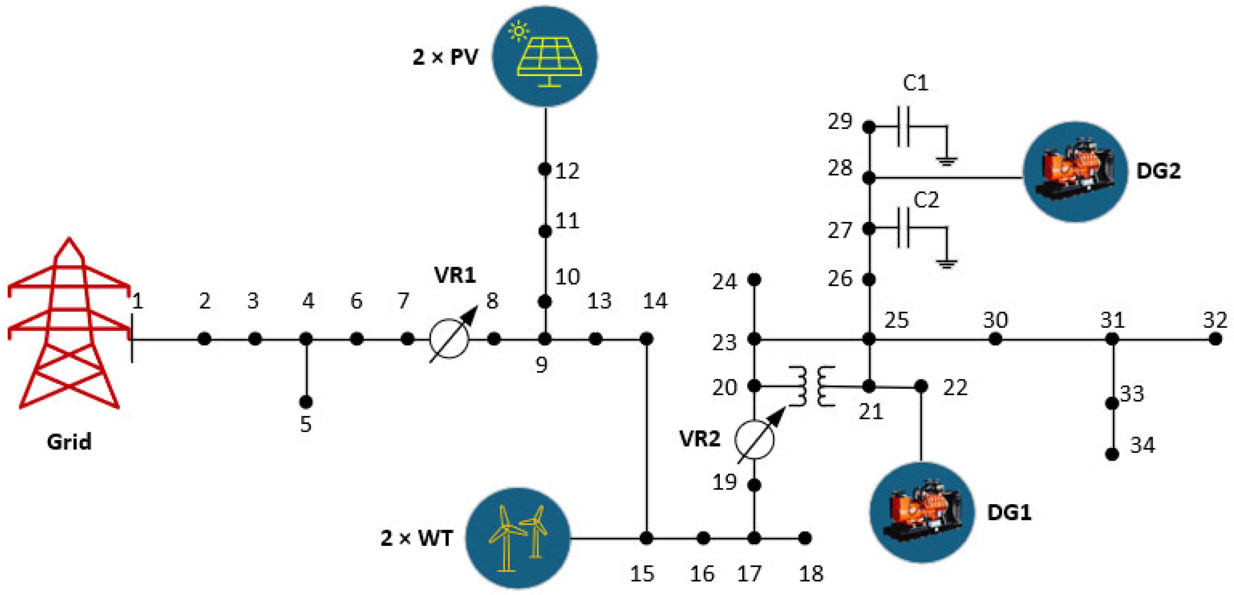
As shown in Figure 8, the proposed strategy is tested in a microgrid that is connected to distributed energy resources (DERs) [2]. These DERs are two diesel generators (DGs), two WTs, and two PV systems. The system serves as a comprehensive model atmosphere for evaluating the performance of the decentralized energy management approach.

Consequently, Buses 22 and 28 will connect the two DG units. Each possesses a distinct cost function, as outlined in

Table 1. Evaluation metrics for LM and RP.

Model	LM				RP
Variable	CC	RMSE	MAD	MAPE (%)	CC	RMSE	MAD	MAPE (%)
Solar Irradiance	0.97	73.21	41.38	8.22	0.97	80.27	46.79	9.84
Ambient Temperature	0.99	0.50	0.41	3.18	0.99	0.71	0.62	4.55
Wind Speed	0.88	1.18	0.92	8.63	0.82	1.38	1.08	10.78
Power Demand	0.68	62.73	49.62	9.39	0.66	62.23	48.89	9.19

. The operational limits of diesel generators for power supply range from a minimum output of 30 MW to 33 MW and a maximum output of 125 MVA to 143 MVA per unit. The operational cost functions of the diesel generators within the system are defined by quadratic cost coefficients. The quadratic cost functions for the DGs are characterized by coefficients a = [0.00043, 0.000394] USD/kWh² and b = [21.6, 20.81] USD/kWh. The coefficients encompass the fuel and maintenance costs associated with diesel generators, incorporating both variable and fixed expenses.

The constraints reflect the actual limitations and operational capacities of distributed generation units within a microgrid. On Bus 15, two wind turbines, each with a rated power of 200 kW, contribute renewable energy to the system. The cost coefficient for wind power generation is 0.1095 USD/kWh, identical to that of the two photovoltaic systems, each with a capacity of 200 kW, located at Bus 12, which also stands at 0.1095 USD/kWh. This indicates comparable economic viability for these renewable energy sources. The microgrid interfaces with the main grid at Bus 1, enabling the importation of power during periods of inadequate local generation. TOU pricing, which varies between peak and off-peak hours, determines the expense associated with importing electricity from the grid. We set the grid power values during peak hours at 0.17 USD/kWh from 1:00 p.m. to 7:00 p.m. Conversely, during off-peak hours, from 7:00 p.m. to 1:00 p.m., the cost is 0.076 USD/kWh. The import of microgrids from the grid is constrained, with a minimum import of 0 kW and a maximum limit of 300 kW.

A DR program equips a microgrid to manage peak demand and enhance grid stability. The demand response program incentivizes load reduction during periods of high demand. The cost coefficient is 0.1 USD per kilowatt-hour for the reduction in load.

5.2. Assessment of Forecast Accuracy

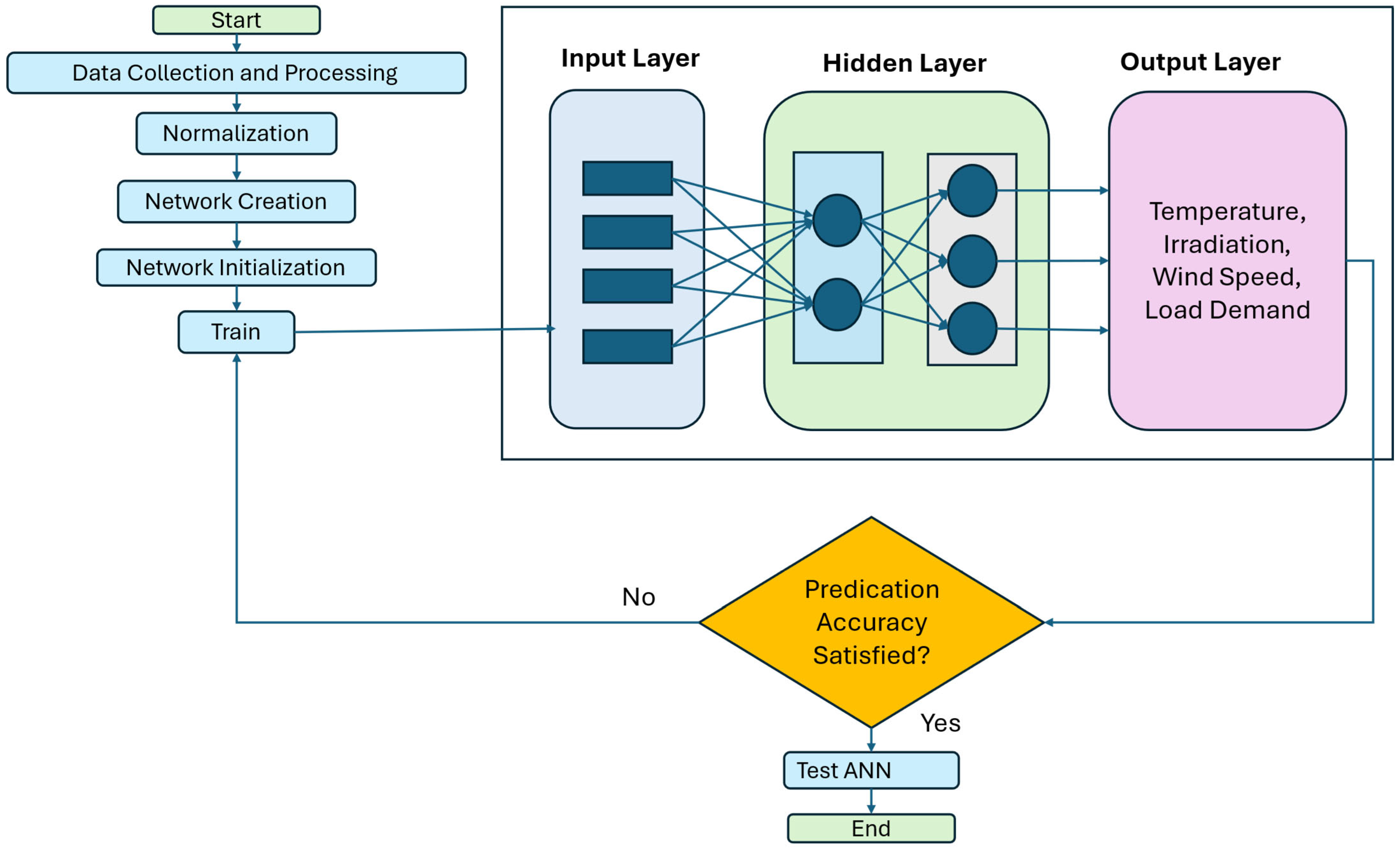
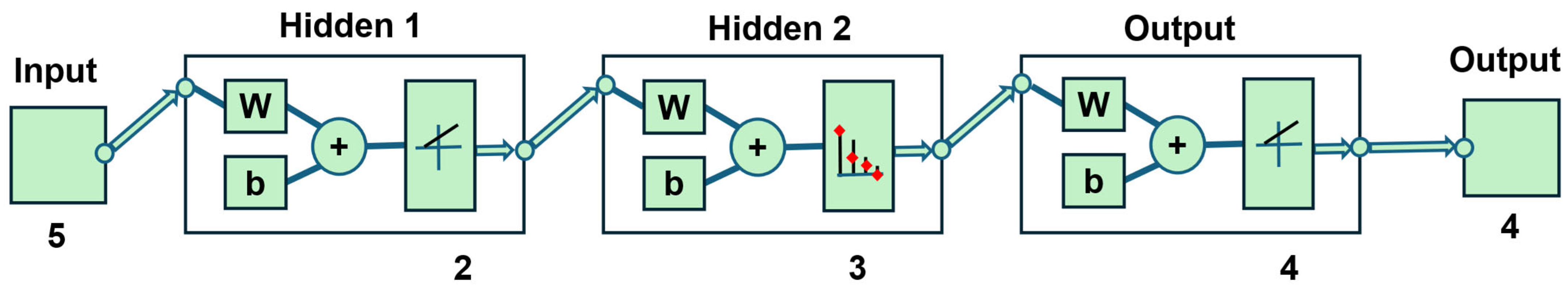
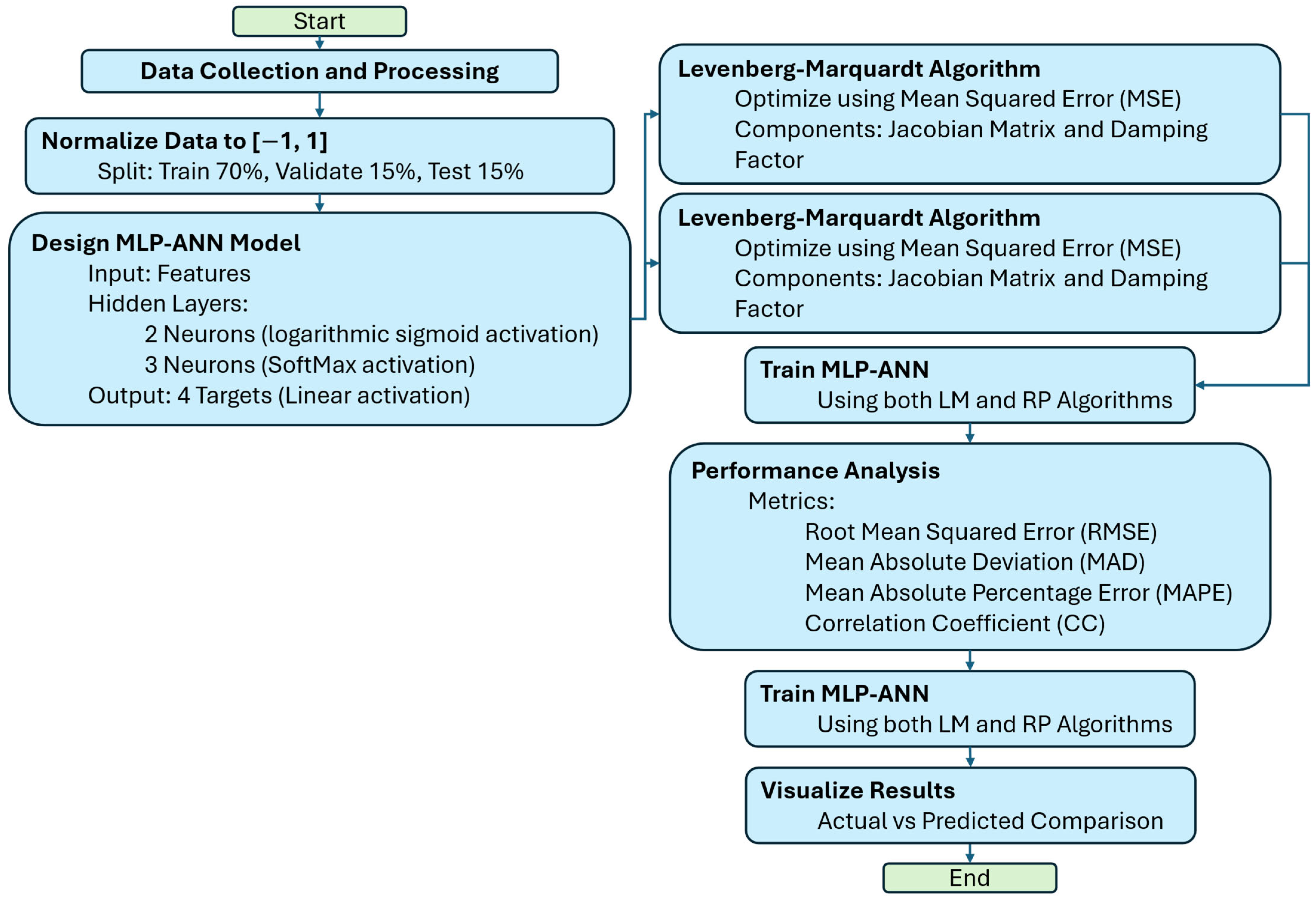
The simulation techniques implemented in a sequential manner displayed the final predictions for solar radiation, temperature, wind speed, and electrical load demand. The two algorithms used were LM and RP. In order to accomplish three consecutive events—training, validation, and testing—the necessary model, MLP-ANN, has been parameterized with variables to be constructed. We have specifically selected a value division ratio of 7:1.5:1.5 based on the dataset. The overall architecture of this model, which executes a total of 600 iterations, consists of the following specifications: two concealed layers, seven input variables, and four output variables. Minimize the training error by employing a minimum-maximum normalization technique for preprocessing.

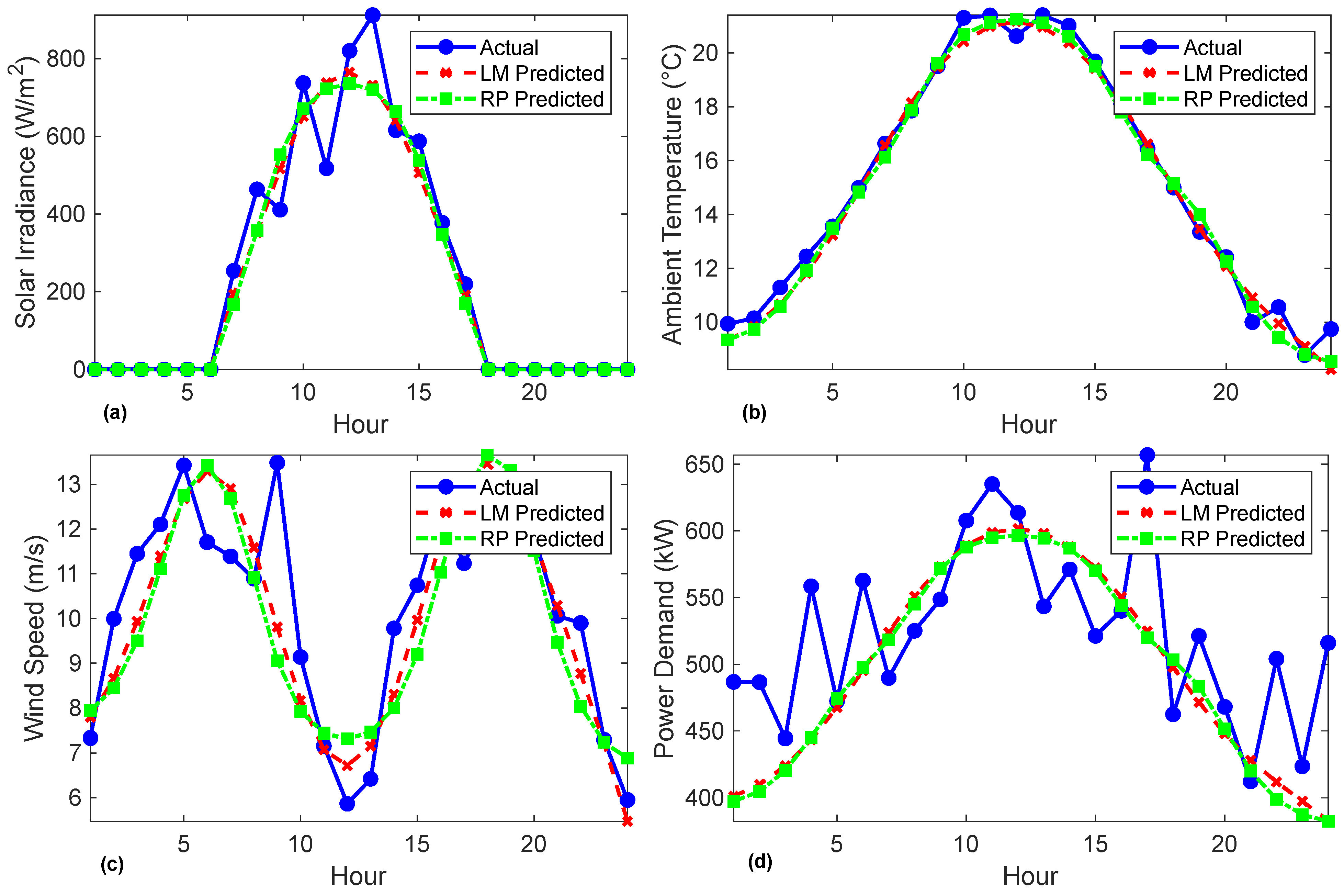
Figure 9 illustrates the predicted and observed values of solar irradiance (a), temperature (b), wind speed (c), and demand (d) for both LM and RP models. The performances of both models are described. Table 1 thoroughly compares the evaluation metrics for both algorithms, incorporating a variety of performance metrics such as the CC, RMSE, MAD, and MAPE for each of the predicted variables.

Table 1 demonstrates that both models readily account for relatively high feasible performances in their forecasts of ambient temperature and solar radiation conditions, which themselves maintain a fair CC > 0.97. Conversely, LM will result in reduced RMSE, MAD, and MAPE when it comes to the precise prediction of the variables selected for solar irradiance and power demand. Conversely, the wind speed and load demand variables do not exhibit any significant differences. Consequently, the models report relatively similar results, with higher error metrics obtained in RP than in LM.

These results also illustrate the LM algorithm’s ability to make more accurate predictions of variables such as solar irradiance and power demand, which could be crucial for energy system optimization. Both models produce outcomes that are highly comparable in terms of ambient temperature, as evidenced by their low RMSE and MAD values. This indicates that temperature can be predicted with relative ease in comparison to the other variables.

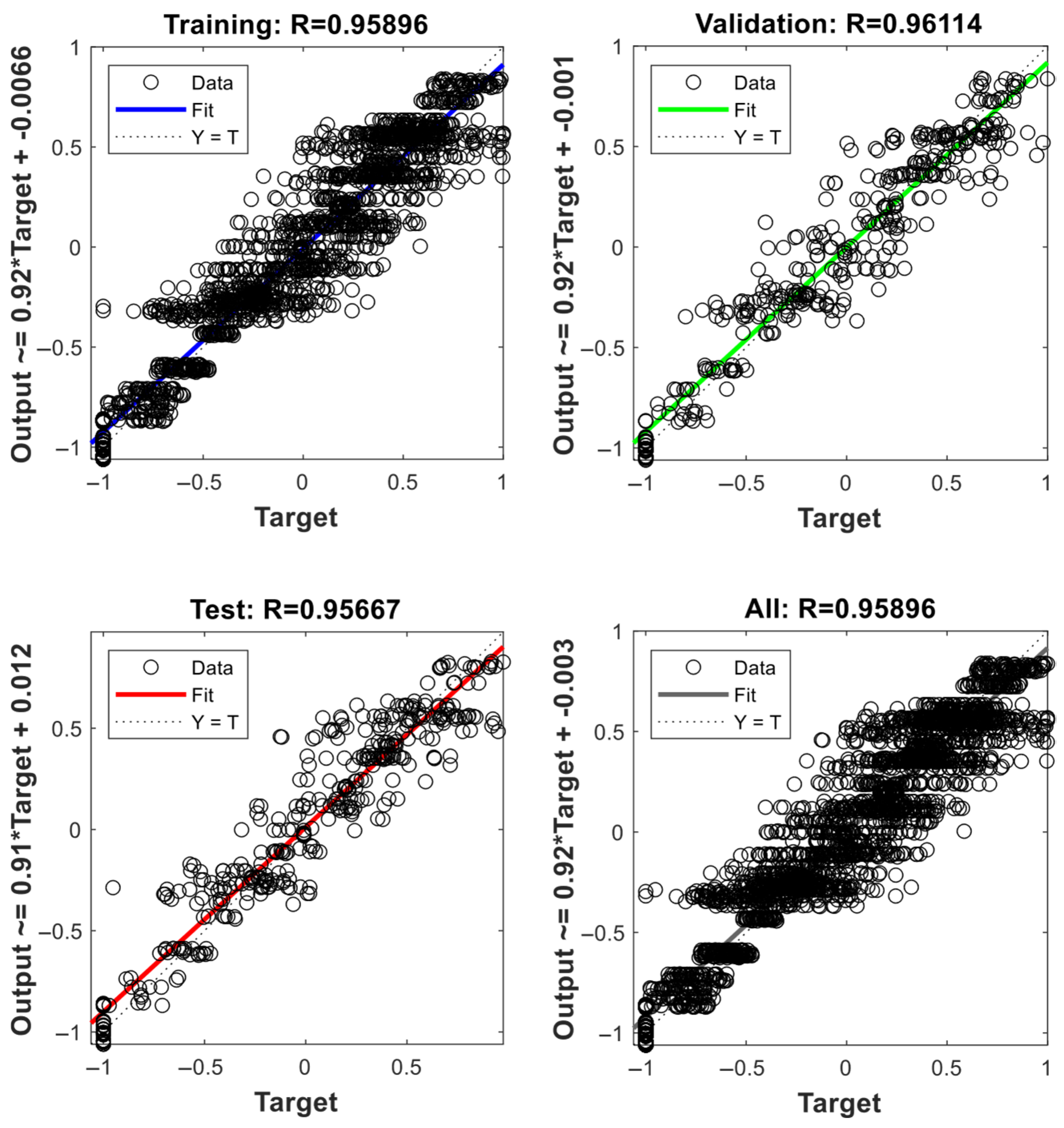
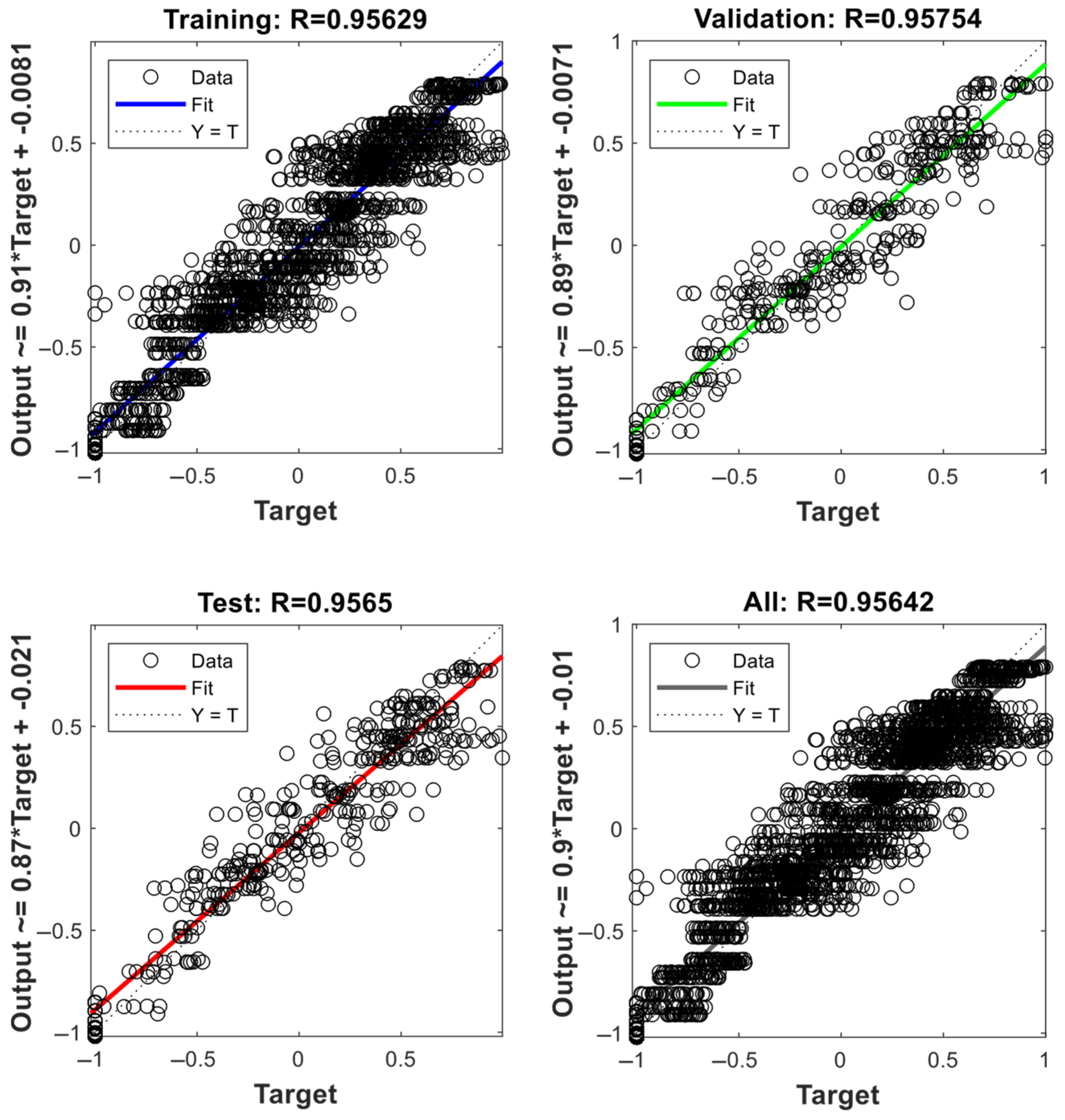
Figure 10 and Figure 11 illustrate the regression between network outputs and actual values for training, validation, and testing, as well as across all datasets, using the LM and RP algorithms. The regression coefficients obtained from the LM and RP models are 0.95896 and 0.95642, respectively, indicating that the LM has greater explanatory power. Observed data is quite consistent with neural network outputs, as evidenced by the strong correlation between predicted and actual values in both models.

The regression plots truly serve as a visual representation of the algorithms’ capacity to identify the fundamental patterns in the data. The degree to which the predictions align with the actual values in both LM and RP truly demonstrates the accuracy of the model. However, LM outperforms RP in this regard. These findings underscore the robust predictive capabilities of the MLP-ANN, bolstering the efficiency of both algorithms in forecasting solar radiation, temperature, wind speed, and load demand.

5.3. Generation Scheduling and Demand Response Initiative

The simulation results of the optimal generation scheduling and load-shifting demand response system targeted at lowest running costs are presented in this part. Three separate cases—each reflecting a different forecasting method and/or renewable energy source—allow us to assess the suggested approach. We reduce the overall expenses related to fuel consumption, generator operation and maintenance, and power procurement from the main grid by means of the MCO algorithm-based optimization of generating schedule.

The three cases analyzed are as follows:

• Case 1: Actual Load and RES
• This case analyzes the efficacy of generation scheduling and demand response programs under actual load and RES situations, devoid of any forecasting methodologies. The system leverages real-time data for both load and renewable energy sources during the operation;
• Case 2: Forecasted Load and RES with LM
• The LM algorithm offers the forecasting for this case, which employs anticipated demand and RES data for system optimization. In this test, we used the LM technique to generate values for upcoming periods, using the predicted output as inputs for optimization;
• Case 3: Forecasted Load and RES with RP
• This case employs the same forecasting methodology as Case 2 but employs the RP algorithm to predict the load and RES data. The RP-based forecasts are subsequently employed to optimize the generation scheduling and DR program, as in the previous case.

This assesses the effectiveness of the proposed MCO-based optimization strategy in reducing operational costs, considering load management strategies and forecasting techniques. The subsequent findings provide a comprehensive analysis of the operational cost, demand response impact, and microgrid performance of each case.

5.3.1. Results of Case 1

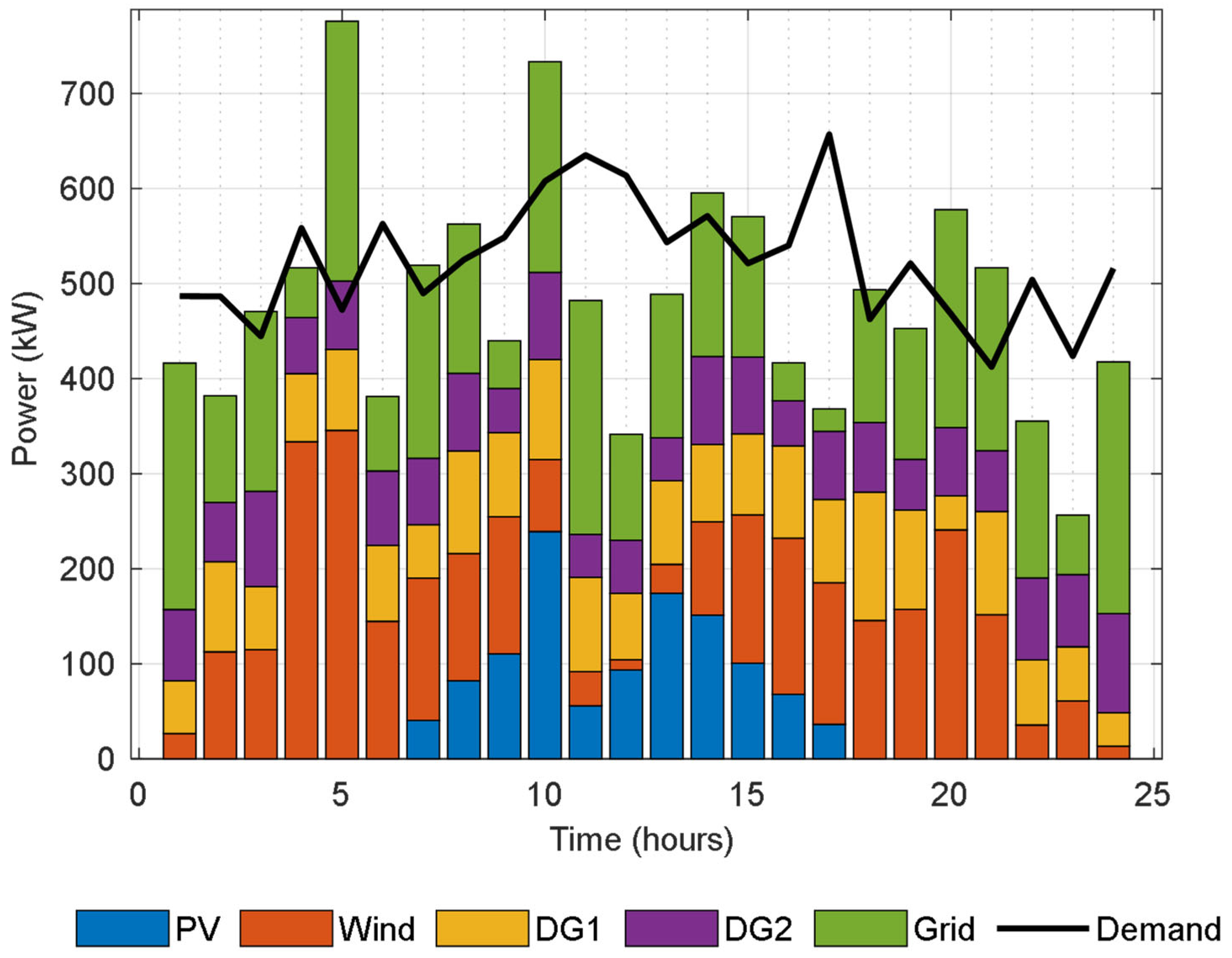
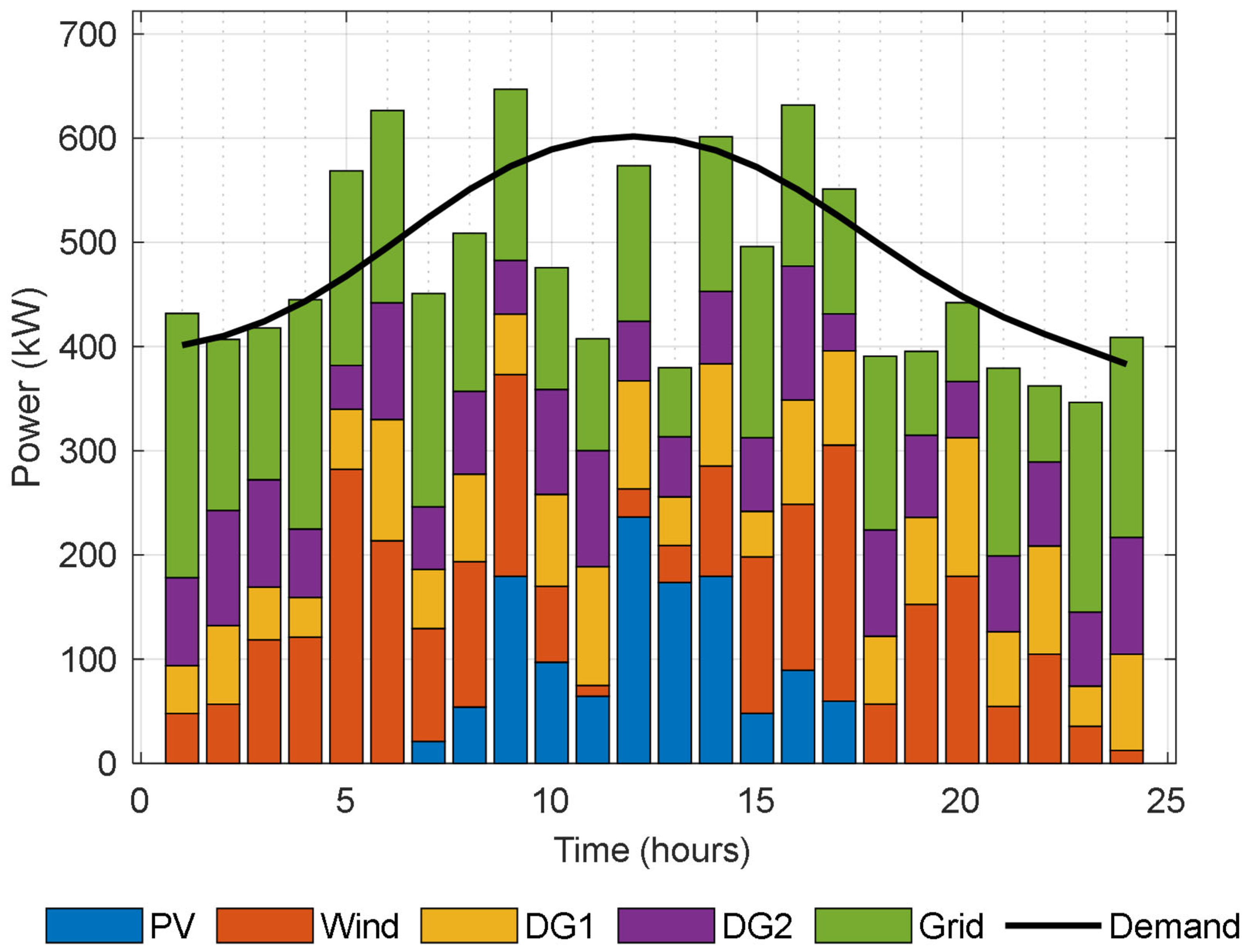
Case 1 presents the optimal generation scheduling for the microgrid using actual load data and the real-time availability of RESs. The contributions of various generation sources, including PV, wind turbines, diesel generators DG1 and DG2, and the main grid over a 24 h period is shown in Figure 12. As can be seen, the integration of renewable energy sources significantly influenced the scheduling strategy, especially during periods of elevated wind or solar generation. For instance, the reliance on diesel generators and grid power significantly decreased during hours with high wind generation, such as hours 4, 5, and 20. Hour 5 saw a peak in wind generation of 345.53 kW, resulting in a significant reduction in demand from DG1 and DG2. During daylight hours, say, at hour 10, PV generation attained 239.15 kW and hence reduced dependence on grid power. On the other hand, during the hours with the least or no renewable generation, such as 1 and 24, there was a significant reliance on DG1, DG2, and grid power to meet the load demand. During hour 1, when wind and PV generation were absent, the load contributions from major participants DG1, DG2, and the grid were 55.58 kW, 74.84 kW, and 259.26 kW, respectively.

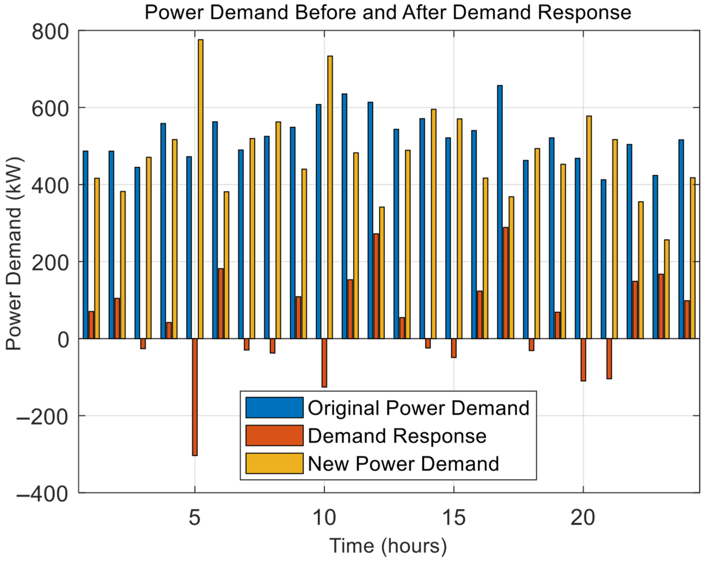
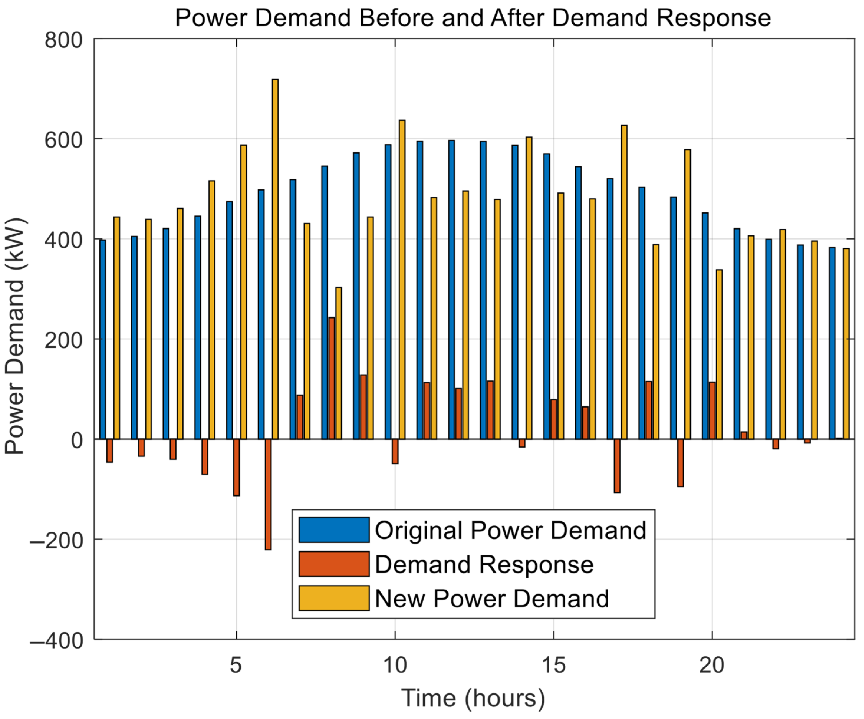
The MCO algorithm will optimize the cost of operation to USD 78,970.35, a significant improvement from USD 110,488.34 without optimization. This reduction has shown the efficiency of the algorithm in the minimization of operational costs by giving a high priority to renewable energy sources and using strategic management for non-renewable generation. We further optimized this by incorporating DR strategies and shifting the load at specific times to optimize resource utilization as indicated in Figure 13. For example, we reallocated 472.34 kW at hour 5 to shift 303.66 kW from that hour to 775.99 kW. At hour 12, the DR strategy shifted 272.11 kW from its original 613.60 kW to a lower 341.50 kW. Overall, the results highlight the potential of the MCO algorithm in handling the variability of renewable energy sources, optimizing operational costs, and leveraging demand response strategies to further improve performance and sustainability of microgrids.

5.3.2. Results of Case 2

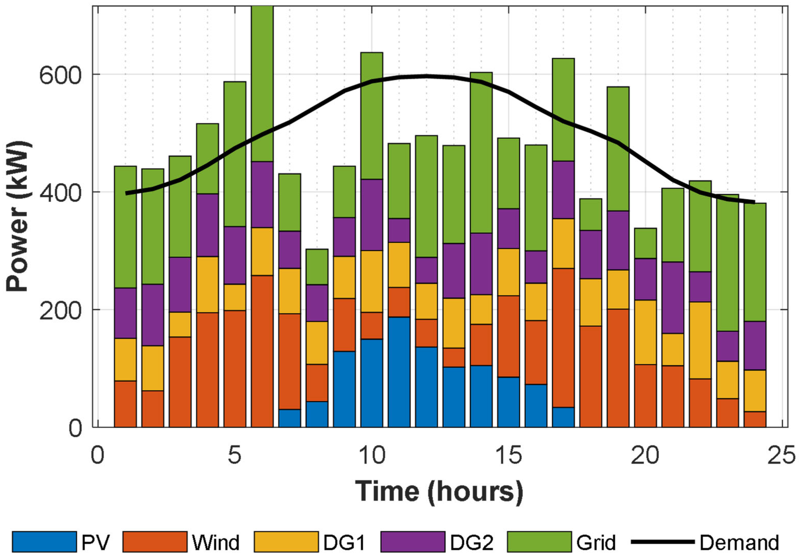
The LM algorithm generates forecasted load and RES data to optimize the generation scheduling of the microgrid in Case 2. Predictive methods delivered highly precise insights for optimization, enabling efficient resource distribution and adaptability in response to the inherent fluctuations in sustainable energy sources. The findings emphasize the impact of various generation sources, including photovoltaic systems, wind turbines, diesel generators (DG1 and DG2), and the primary grid over a 24 h timeframe as shown in Figure 14.

Enhancements related to the fluctuations in the inputs from renewable sources, a crucial factor in the formulation of scheduling approaches, have enabled efficient management. Indeed, during times of increased availability, particularly noticeable at hour 9, the peak output from wind sources soared to 193.58 kW, complemented by a substantial contribution of 179.53 kW from photovoltaic systems. As a result, the resources highlighted played a crucial role in minimizing reliance on dispatchable units and grid imports. The dispatchable units, DG1 and DG2, produce only 57.99 kW and 51.64 kW, respectively, and the grid can only sell 164.17 kW. Hour 14 saw the peak of RES contributions, with PV producing 179.53 kW and wind generating 105.80 kW. Consequently, we capped the outputs for DG1 and DG2 at 98.03 kW and 69.52 kW, respectively, and minimized the import from the grid to 148.53 kW. The results demonstrate that the system can prioritize sustainable utilization, reduce operational costs, and improve scheduling efficiency.

During times of diminished generation from sustainable sources, the model responded by enhancing its dependence on traditional energy sources and grid imports to satisfy the demand for power. During the first hour, with no photovoltaic generation and a slight wind input of 47.77 kW, DG1 and DG2 provided 45.91 kW and 84.50 kW, respectively, while the grid fulfilled the remaining demand with 253.63 kW. During hour 23, the wind generation decreased to 35.58 kW, with no PV availability. This situation necessitated increased outputs from DG1 and DG2, approximately 38.57 kW and 71.00 kW, respectively, along with grid imports of 201.15 kW. These examples illustrate the model’s ability to adaptively redistribute resources to guarantee optimal load satisfaction in response to changing circumstances.

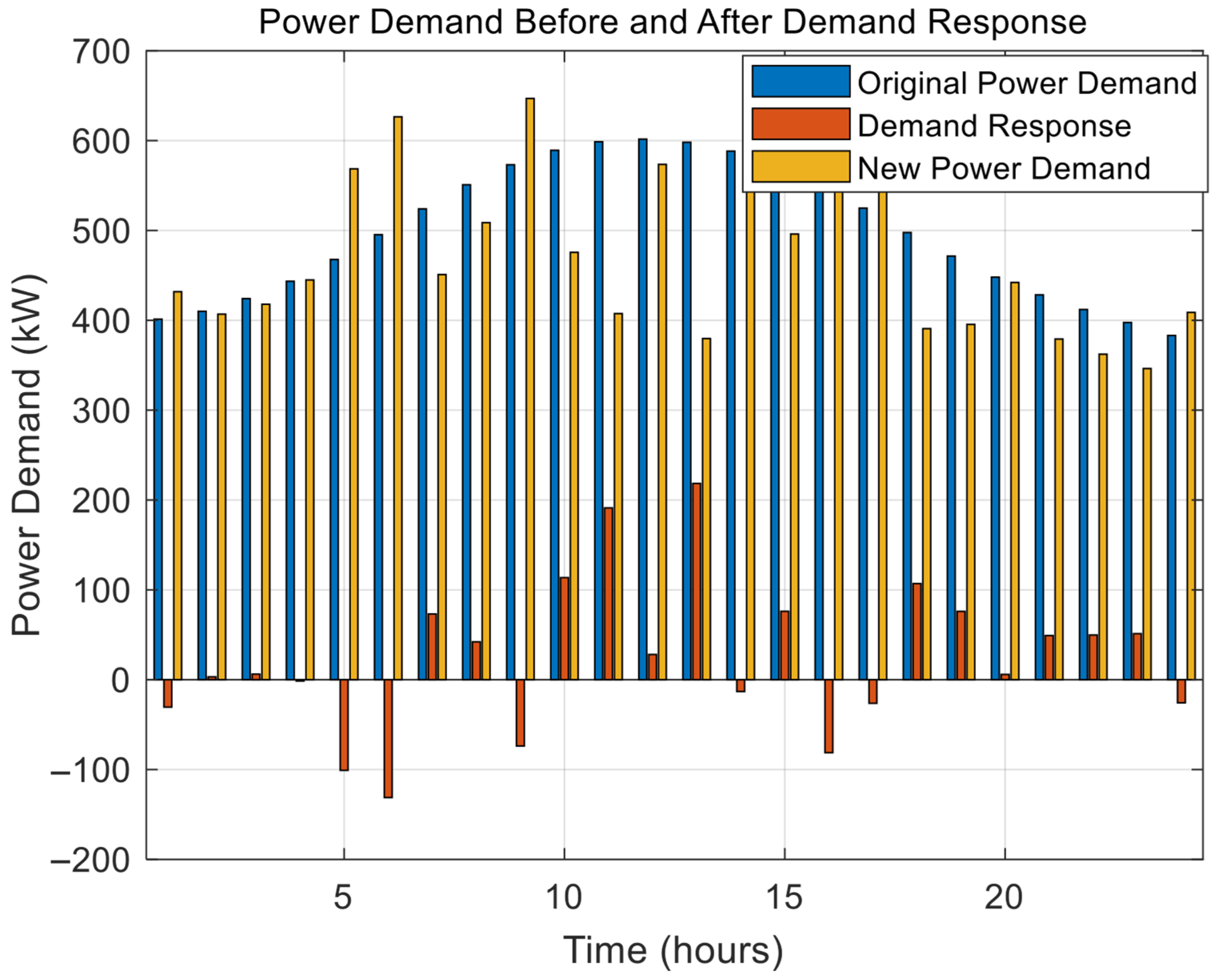
As illustrated in Figure 15, the incorporation of demand response strategies enhanced the system’s performance by adjusting the loads according to operational conditions. For example, a decrease of 131.18 kW in load during hour 6 alleviated pressure on the system, while an increase of 191.22 kW during hour 11 promoted more effective use of excess clean energy production. This approach will synchronize the load profile with generation availability, leading to a decrease in dependence on grid power and fossil fuels while enhancing overall efficiency.

This resulted in significant reductions in the unoptimized operating expenses, totaling USD 110,488.34. Through optimization, LM-based forecasting and demand response have significantly boosted operational efficiency, resulting in substantial cost reductions and enhanced management of resources. This result shows how important predictive modeling and resource optimization are for dealing with the unpredictable nature of clean energy sources. This improves the microgrid’s operational reliability, long-term viability, and cost-effectiveness.

5.3.3. Results of Case 3

Case 3 illustrates the generation scheduling optimization problem by using forecasted demand and RES predicted by the Resilient Backpropagation algorithm. Using these RP-based forecasts as input provides a reliable and effective foundation for the efficient scheduling of resources, seamlessly integrating demand response. This has demonstrated that the system dynamically adjusts to fluctuations in renewable energy availability, utilizing dispatchable resources in a manner that is both economical and stable.

Throughout the 24 h period, as shown in Figure 16, the optimized scheduling guarantees the most efficient utilization of renewable energy sources, particularly wind and photovoltaic systems, during peak generation hours. For instance, it lessens dependence on grid power and dispatchable units during the peak hour of wind generation, which is 257.83 kW at hour 6. Therefore, we assume that DG1 and DG2 produce medium-level outputs of 81.48 kW and 112.17 kW, respectively, and achieve load balancing by importing 267.09 kW from the grid. Consequently, this diagram endeavors to illustrate the potential for resource utilization that is more efficient because of the increased availability of renewable energy sources. The 236.01 kW increase in wind generation at hour 17 further reduces the dependency on the grid to 174.36 kW. The sharing of dispatchable units is also effective, with 84.67 kW from DG1 and 97.90 kW from DG2. The system’s ability to adapt to the fluctuations in renewable energy sources guarantees economical and dependable operation, particularly when renewable energy is abundant.

Simultaneously, PV generation has the potential to significantly reduce grid dependence, particularly during midday. The combined shares reduce grid imports to 127.49 kW and DG1/DG2 feed at a reduced amount of 76.54 kW and 40.50 kW, respectively, at hour 11, when they achieve its peak value of 187.35 kW with the help of 50.31 kW from wind output. This guarantees a decrease in operating costs and reliance on nonrenewable sources by optimizing the utilization of variable renewable resources.

When renewable energy generation is insufficient, the system responds by increasing its reliance on dispatchable units and grid imports. For instance, at hour 1, there is no PV generation and a restricted wind output of 78.69 kW. DG1 and DG2 supply 72.54 kW and 85.49 kW, respectively, while grid imports increase to 206.89 kW. Similarly, at hour 23, the wind generation declines to 48.66 kW, while there is no PV output. In addition to 232.36 kW grid imports, the system has now increased DG1 and DG2 to 63.60 kW and 50.91 kW, respectively. The system consistently implements these modifications to meet demand, even during periods of low renewable availability.

The DR program, as shown in Figure 17, improves the system’s performance by adjusting the load in accordance with operational conditions. For instance, the program reduces operational costs by reducing peak demand and adjusting the load profile to match generation availability, thereby reducing reliance on grid imports and dispatchable units. In this manner, incorporating DR will ensure the system remains cost-effective even in the face of adversity.

As a result, Case 3 optimizes its operating cost, demonstrating the effectiveness of RP-based forecasting and integrated DR strategies. Consequently, the operating cost significantly decreases compared to unoptimized scenarios. These results underscore the system’s resilience in managing the variability of renewable energy sources, ensuring reliable operation and minimal costs while optimizing the efficient integration of renewable energy sources.

5.3.4. Total Power Generation in the Case Studies

This section contrasts the total power generation of the three case studies, emphasizing the interaction between grid imports, local generation, and the impact of the demand response program. The findings offer a comprehensive understanding of the impact of the optimization strategies in each case on the utilization of local resources and the overall power generation.

In Case 1, as represented in

Table 2. Total power generation in the case studies.

Case #	Gird (kW)	Local Gen. (kW)	DR Total (kW)
Case 1	3680.001456	7850.774091	1041.677698
Case 2	3690.546699	7653.857775	607.1113135
Case 3	3943.648099	7598.336085	355.9692446

, the maximum generation and DR contribution are presented as follows: Local generation is 7850.77 kW, and the total DR is 1041.68 kW. In this instance, the grid imports amount to 3680.00 kW, which suggests a significant reliance on local generation and DR programs to satisfy the demand. As the local generation decreased to 7653.86 kW, Case 2 indicates a minor increase in grid importation to 3690.55 kW. Additionally, the DR total decreased to 607.11 kW. Therefore, despite nearly identical grid importation, it is reasonable to infer a diminished contribution from the DR program compared to Case 1. Case 2’s optimization strategy is to blame for this. Case 3 further increases utility imports to 3943.65 kW, while local generation marginally decreases to 7598.34 kW. The reduction in the total DR in Case 3 to 355.97 kW further demonstrates the reduced role of demand response in load balancing. This trend is consistent with the other cases.

Throughout the three cases, the fluctuations in grid import, local generation, and the DR contribution demonstrate how each scenario has responded to varying levels of renewable energy, a distinct approach to load forecasting, and, as a result, the effectiveness of the demand response strategy in optimizing the cost of total power generation.

5.3.5. Analysis of Operational Costs

The operational costs of generation sources are assessed over a 24 h period in four scenarios: without optimization (wo/optimization) and three optimization cases (Case 1, Case 2, and Case 3). The results of

Table 3. Operational costs (USD/h) of the generation sources in the cases.

Time (h)	wo/opt	Case 1	Case 2	Case 3
1	4016.49901	2791.127	2775.326	3370.753
2	4012.299966	3380.883	3957.249	3854.598
3	3415.209351	3547.918	3265.85	2886.221
4	5514.428394	2822.845	2223.335	4311.081
5	3715.604693	3372.593	2156.397	3041.558
6	5605.418322	3399.249	4880.023	4128.463
7	4078.380805	2706.178	2514.636	3025.003
8	4845.054157	4082.725	3523.624	2926.634
9	5337.48599	2928.058	2390.988	2974.416
10	5745.957024	4246.864	4058.731	4853.323
11	5748.957753	3155.872	4837.422	2558.217
12	5746.599395	2729.704	3493.648	2308.117
13	5228.080859	2897.346	2268.99	3829.498
14	5741.948459	3743.277	3625.395	3336.166
15	4764.706964	3574.969	2475.976	3200.479
16	5157.624	3135.079	4891.306	2574.407
17	5751.342471	3441.607	2745.905	3921.388
18	3538.947464	4487.293	3580.845	3492.784
19	4736.03933	3409.708	3482.03	3563.465
20	3625.319983	2303.714	4031.57	3875.136
21	2456.36054	3701.873	3089.849	3743.393
22	4377.830472	3308.831	3951.49	3917.054
23	2700.935559	2841.413	2337.571	2458.137
24	4627.31293	2961.224	4351.358	3271.488
Total cost	110488.3439	78970.35	80909.51	81421.78

illustrate the significant influence of optimization strategies on the reduction in costs and the enhancement of efficiency.

In Case 2, we used the LM algorithm to obtain the forecasted load and RES data, which led to an operational cost of USD 80,909.51. This represents a reduction of approximately 26.8% from the baseline of USD 110,488.34. Case 3 employed the RP algorithm to forecast load and renewable sources data, leading to a reduction of approximately 26.3% in the total cost of USD 81,421.78. These findings demonstrate the extent to which sophisticated forecasting algorithms can optimize generation scheduling and reduce uncertainties.

Table 4. Comparison of operational cost reduction between the proposed method and the State-of-the-Art results.

Method	Uncertainty	Operating Cost Reduction (%)
[34]	PV uncertainty	15.6%
[43]	Not considered	5%
[44]	Wind uncertainty (10%)	27%
[45]	Price uncertainty	16%
[3]	11% PV uncertainty, 10% wind uncertainty	23%
Case 2	Forecasted Load and RES with LM	26.8%
Case 3	Forecasted Load and RES with RP	26.3%

emphasizes the competitiveness of Cases 2 and 3 by contrasting the results with the existing literature. For instance, in [34], the authors achieved a 15.6% cost savings by considering the uncertainty in PVs’ demand response and energy storage. In [43], the authors achieved a 5% reduction by employing load-shifting strategies without resolving system uncertainties. In contrast, Case 2 and Case 3 have accomplished more substantial reductions by integrating uncertainty modeling with LM and RP algorithms, respectively. Similarly, Case 2’s cost savings of 26.8% and Case 3’s cost savings of 26.3% surpasses the 16% reduction reported in the study, which optimized a network–load interaction framework to capture pricing uncertainty. Additionally, the model incorporated wind uncertainty and demand response, resulting in savings of 27%. These results are consistent with the performance of Cases 2 and 3 under the more comprehensive modeling of uncertainty.

In Cases 2 and 3, the operationalized proposed approach aligns with the forecasting results of the ARIMA model, leading to a 22% cost reduction. Nevertheless, the LM-based and RP algorithms that were implemented in Cases 2 and 3 demonstrated a greater ability to adjust to system uncertainties in order to achieve optimal conditions for the local generation scheduling applications while simultaneously balancing demand-side management algorithms. This behavior suggests that the optimization modeling methodology is effective in mitigating uncertainties related to renewable energy use and load preconditioning.

The test system (Figure 8) validated the EMS’s efficacy, with MCO achieving a 26.8% cost reduction (Table 3) and DR programs enhancing load flexibility (Figure 13, Figure 15 and Figure 17). Case 2 (LM forecasting) showed superior accuracy, underscoring the importance of precise predictions. The comparison study showed that using advanced forecasting algorithms along with demand response strategies can effectively lower operational costs, even when there are a lot of unknowns. The substantial cost reductions that Case 2 and Case 3 generated among all the optimized cases demonstrated the effectiveness of utilizing predictive algorithms for energy management in modern power systems.

5.4. Comparison with Other Algorithms

The demand response program’s implementation within the microgrid led to substantial reductions in peak load and enhanced load balancing. This adaptability enabled the microgrid to enhance its overall resilience and stability by dynamically adapting to fluctuations in demand and generation.

The proposed system has been evaluated in comparison to four well-known optimization algorithms: MCO, CO, PSO, and TLBO. Each algorithm was executed once, with a population size of 10, a maximal number of iterations of 100,000, and a total of 25 trials. Key performance trends are emphasized within the summary of the results from three distinct cases as represented in

Table 5. Statistical results of optimal EMS using different algorithms in case studies.

Case #	Metric	MCO	CO	PSO	TLBO
1	min	7.90 × 104	8.63 × 105	8.08 × 106	2.32 × 106
	mean	2.17 × 106	2.73 × 107	5.80 × 107	1.54 × 107
	max	3.55 × 1011	3.71 × 1012	2.09 × 1013	4.33 × 1012
	SD	8.02 × 104	1.76 × 1012	1.96 × 1013	4.67 × 1012
2	min	80,909.53	21,894,794	4.3 × 108	96,116,699
	mean	4,610,438	26,485,154	58,549,038	14,268,439
	max	1.7 × 1011	3.16 × 1012	1.19 × 1013	2.98 × 1012
	SD	94,543.7	3.18 × 1012	2.21 × 1013	5.92 × 1012
3	min	81,490.88	134,489.5	824,219.3	168,877.8
	mean	5,944,093	24,715,388	41,816,119	11,115,255
	max	1.43 × 1012	4.9 × 1012	2.65 × 1013	5.79 × 1012
	SD	78,730.35	5.87 × 1011	4.13 × 1012	1.34 × 1012

.

In Case 1, MCO demonstrated its efficiency in cost minimization by generating the minimum and mean values of operation costs for all scenarios. In comparison to other algorithms, the SD value of MCO is also exceedingly small, which demonstrates that the convergence of MCO is more consistent. In contrast, the other three algorithms, namely CO, PSO, and TLBO, exhibit a significantly higher operational cost and a greater degree of variability in their results. Their standard deviations are significantly greater than those of MCO. MCO maintained its optimal performance in Case 2. The average costs of CO and TLBO were higher, resulting in poorer operating practices, as well as higher standard deviations. PSO exhibited an even greater degree of variability; its maximal operational cost and SD were all higher than those of other algorithms. The robustness of the system in managing uncertainty was underscored by the smaller mean and SD of MCO. MCO once again surpassed the other algorithms compared in Case 3 by providing the minimum average operational cost with the least standard deviation. This implies that it not only ensures a superior performance in terms of cost, but also reliable results after repeated trials. The PSO and TLBO have led to a relatively higher cost with greater variability, particularly in terms of maximal cost and standard deviation.

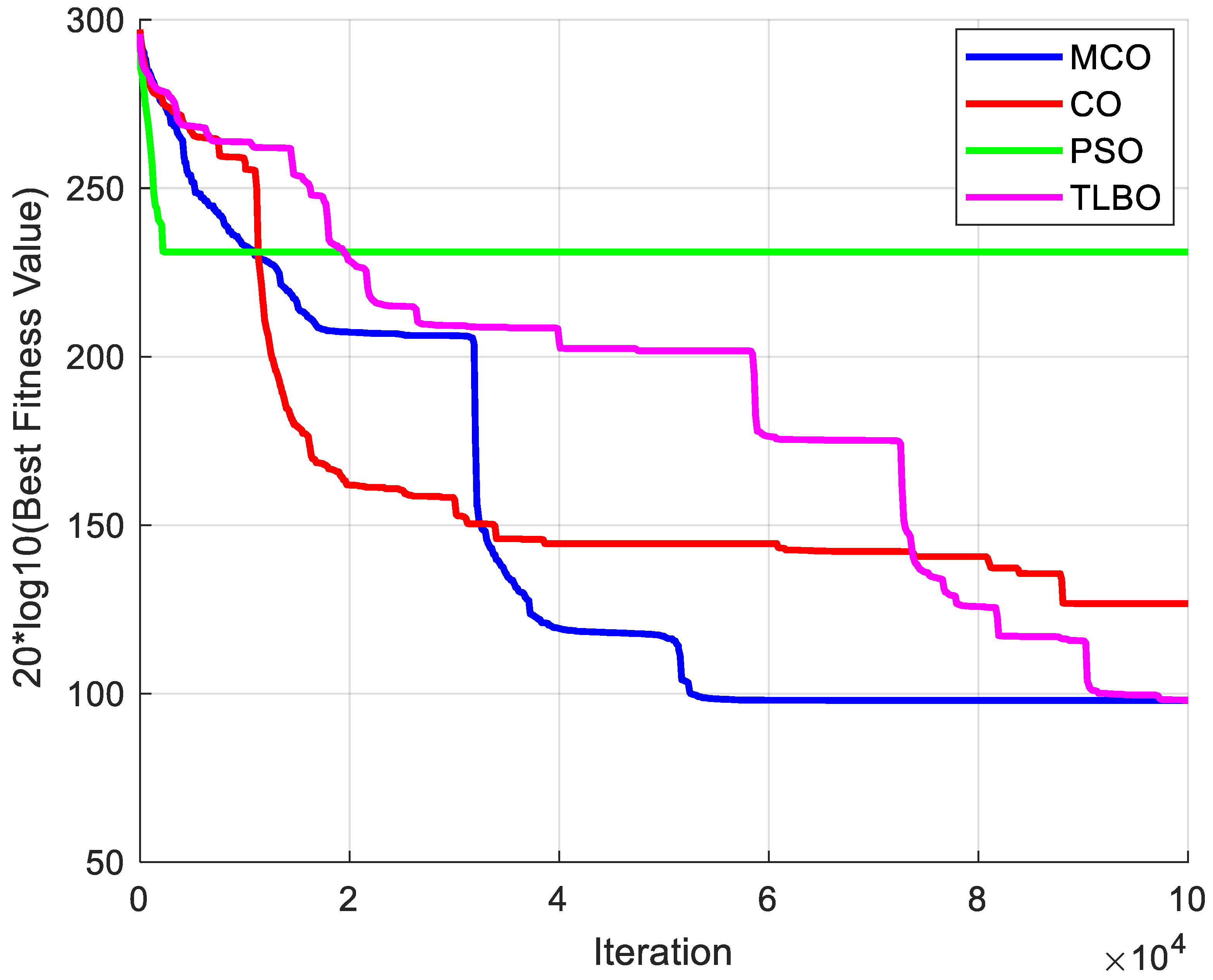
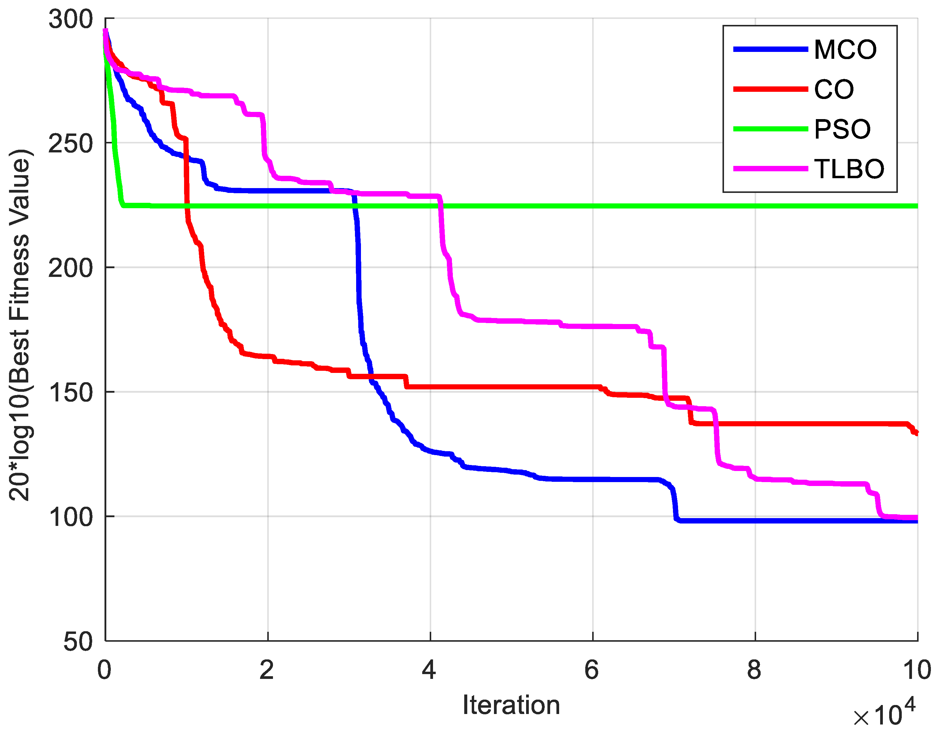
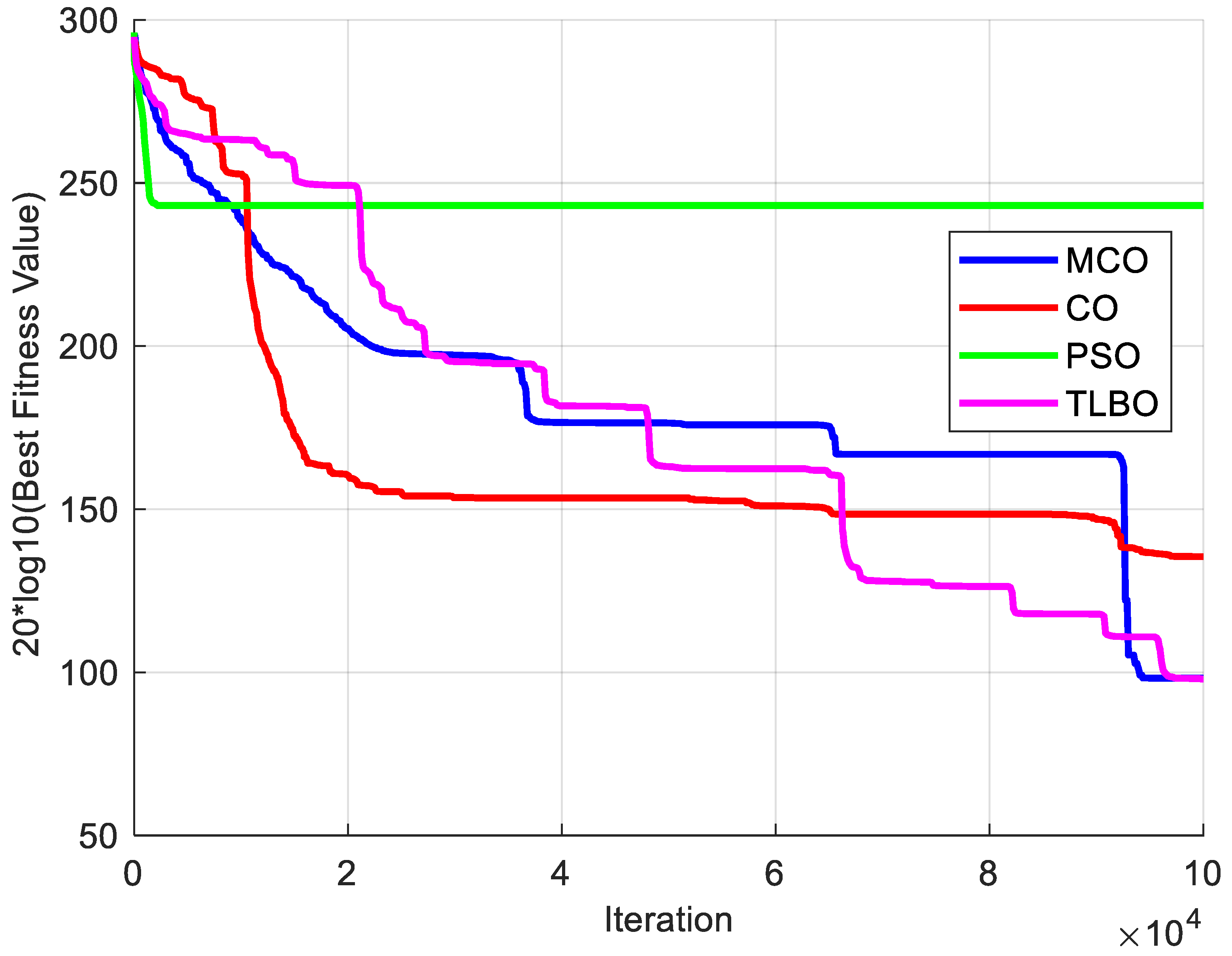
Figure 18, Figure 19 and Figure 20 illustrate the convergence trajectories of the algorithms for the optimal run over 25 trials. The convergence behavior of each algorithm during the optimization process is illustrated in these diagrams. PSO has consistently converged to suboptimal solutions and has converged prematurely in all trials. It was unable to evade local optima and was found to be the least efficient algorithm in terms of convergence efficiency. Conversely, CO achieved a higher convergence rate during the initial iterations than TLBO and MCO. Nevertheless, CO was unable to investigate superior solutions during subsequent optimization iterations, as it converged to a local optimum. In both Cases 1 and 2, it is evident that MCO converges more rapidly, and TLBO was outperformed by avoiding local optima. In Case 3, both TLBO and MCO exhibited a comparable convergence trend; however, MCO achieved a marginally faster convergence rate.

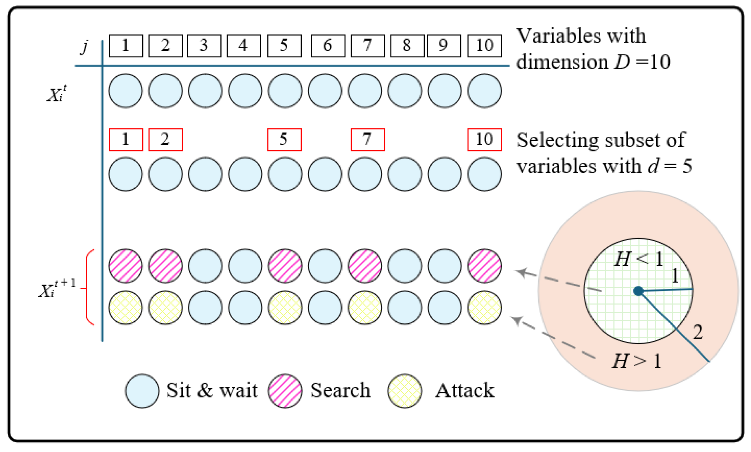
In general, the efficacy of MCO has been superior in all three cases. MCO is more stable and efficient, as evidenced by the minor deviations from the minimum operational cost in all three cases. This conclusion can also be drawn from the convergence behavior illustrated in the subsequent figures, which demonstrate that MCO has superior convergence. Specifically, it identifies the optimal solution with greater speed and reliability than other algorithms. Its successful operational management was significantly influenced by the integration of demand response with an optimal scheduling approach, as well as modifications to the MCO algorithm. The balance between exploration and exploitation is improved in the improved MCO algorithm by simplifying the randomization and turning factors, H value, and presenting an improved search strategy that utilizes the leader’s position. Consequently, MCO possessed a robust and adaptive search process that was more cost-effective and stable than the other algorithms.

5.5. Robustness Analysis Under Operational Uncertainties

To strongly evaluate the suggested MCO algorithm under realistic uncertainties, an extensive sensitivity study was conducted, considering large fluctuations in both renewable generation and loading demands. Detailed test scenarios were carefully defined to ensure that abnormal operating situations that can be experienced by microgrids were effectively addressed, including excess renewable generation, energy shortages, and volatile fluctuations.

The test cases included a variation of about ±30% in output produced by photovoltaics and wind farms, plus associated variations in demand, giving three specific test cases: high renewable generation and low demand (HRLD), low renewable generation and high demand (LRHD), and anomalous volatility in both factors (VF). These cases were tested using the same 600 kW test microgrid described in Section 5.1, with a data resolution period of 1 min over a 30-day test period.

Table 6. Comparative performance under ±30% perturbation scenarios.

Algorithm	Nominal Case (USD)	HRLD Scenario (USD)	LRHD Scenario (USD)	VF Scenario (USD)	Cost Savings vs. PSO (%)	Constraint Violations
MCO	78,970	78,420	82,150	80,790	24.1–27.5	0
PSO	110,488	85,330	92,410	89,120	Baseline	12
GA	110,488	88,760	95,830	92,450	15.8–19.4	19
TLBO	110,488	83,910	90,250	87,680	20.1–23.9	8

shows that the MCO algorithm was considerably effective in all experimental scenarios. Under the less complex HRLD scenario, the algorithm effectively minimized operating costs to USD 78,420, which is a reduction of 26.1% compared to traditional methods. Under the larger-scale LRHD scenario, the MCO algorithm limited cost rises to only 4.2% compared to conventional methods, while achieving a reduction of 24.3% compared to baseline methods. Under the VF scenario, which assumes realistic grid scenarios, moderate effectiveness was realized, and the MCO algorithm significantly exceeded all baseline algorithms.

Notably, the energy management system based on MCO fully preserved all operating constraints in the testing period, involving power balance requirements and generation limits. This superior constraint satisfaction is in sharp contrast to the performance exercised using PSO (12 violations), GA (19 violations), and TLBO (8 violations) under identical testing scenarios. The capable performance can be related to the algorithm’s strategy selection dynamic mechanism as well as its adaptive balance between exploration and exploitation, which promote effective search navigation in the solution space, even in the presence of substantial parameter variations.

The results offer significant validation for the practicability of the proposed methodology, particularly for applications related to microgrids involving high penetration of renewable energies and variable demand.

The robustness analysis supports the claim that the MCO algorithm can preserve its performance advantage, even under significant uncertainties present in the system. This attribute makes it particularly suitable for real-world microgrid applications, where prediction errors and demand variability are unavoidable. The outcomes agree with the existing literature on managing uncertainties in renewable systems, while showcasing improved performance properties over conventional methods presented in [19,20]. The consistent performance of the algorithm under varied conditions presents a positive prospect for real-world applications in microgrids, where reliability in uncertain environments is a major consideration.

6. Conclusions

This paper proposes a complete decentralized energy management system (EMS) for microgrids, integrating Multi-Layer Perceptron Artificial Neural Network (MLP-ANN) prediction with a new Modified Cheetah Optimizer (MCO) algorithm. The main contributions and results are presented below:

• The LM-trained MLP-ANN achieved superior prediction accuracy (8.22% MAPE for solar irradiance, 9.39% for load demand) compared to RP training and traditional statistical methods, enabling more reliable renewable energy integration;
• The suggested MCO algorithm demonstrated significant advantages over PSO, GA, and TLBO, obtaining a 26.8% decrease in operating costs while satisfying all constraints for every test scenario;
• Extensive sensitivity analyses confirmed MCO’s stability under ±30% renewable generation and demand fluctuations, with cost deviations limited to 24.1–27.5% savings even in worst-case conditions;
• The implemented DR strategy successfully reduced peak loads by 7.5% through dynamic pricing models, contributing to improved grid stability and economic efficiency.

Despite the model’s production of positive end-states, various shortcomings highlight important future research directions:

• The current validation on a 600 kW microgrid requires extension to larger systems (>5 MW) with more distributed energy resources to fully assess operational scalability;
• Though high-resolution (1 min) simulations were conducted, hardware-in-the-loop testing using platforms like Opal RT Simulator is needed to verify real-time performance and operational cost dynamics in physical microgrid testbeds;
• The MLP-ANN’s 24 h prediction horizon should be expanded to multi-day forecasting to better support seasonal energy planning and operational scheduling;.
• Future work will incorporate electric vehicle charging loads as flexible response resources while optimizing battery cycling costs, enhancing the EMS’s adaptability to evolving grid architectures;
• Studies should look at the integration of emerging technologies, including fuel cells and hydrogen storage systems, to fulfill energy-balancing needs over long periods.

Such innovations will manage substantive gaps between theory development advancements and applications, particularly in reference to microgrids operating in situations involving high renewable energy penetration. The proposed MCO-based methodology sets an effective foundation for such endeavors, showcasing both tech benefits as well as financial efficiencies for sustainable energy systems inclusion.