


Analysis of Spatiotemporal Characteristics of Microseismic Monitoring Data in Deep Mining Based on ST-DBSCAN Clustering Algorithm

 ,
,
Abstract
1. Introduction
2. Materials and Methods
2.1. Related Concepts
- (1)
- ε-Neighborhood: For a sample point p, the point’s ε-neighborhood is defined as the set of all sample points within a distance less than or equal to ε from p.
- (2)
- Core Point: Within an ε-neighborhood (defined by a radius ε), if a sample point has at least MinPts (a minimum number of samples) within its ε-neighborhood, it is termed a core point.
- (3)
- Border Point: A sample point p is a border point if the number of samples in its ε-neighborhood is less than MinPts but p lies within the ε-neighborhood of some core point.
- (4)
- Noise Point: A noise point is a sample point that is neither a core point nor a border point.
- (5)
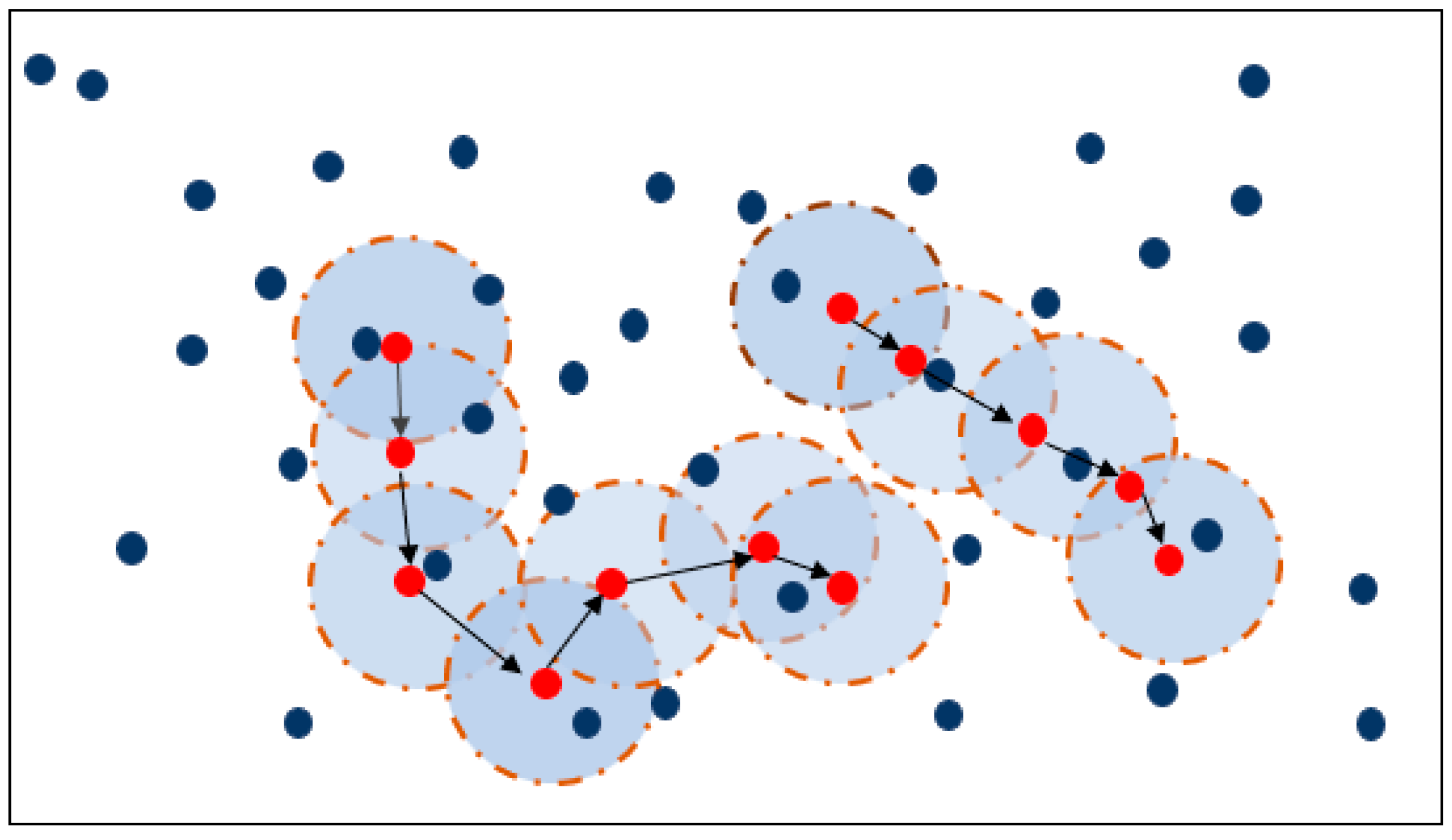
- Directly Density-Reachable: If a point q lies within the ε-neighborhood of a core point p, then q is directly density-reachable from p.
- (6)
- Density-Reachable: A point q is density-reachable from a point p if there exists a sample chain (p1, p2, …, pn) where (p1 = p), pn = q, and each pi+1 is directly density-reachable from pi.
- (7)
- Density-Connected: Two points p and q are density-connected if there exists a core point o, such that both p and q are density-reachable from o.
- (8)
- Cluster: A cluster is a maximal set of density-connected sample points satisfying the following conditions: any two points within the cluster are density-connected, and the cluster contains at least one core point.
2.2. ST-DBSCAN Algorithm: Steps
- (1)
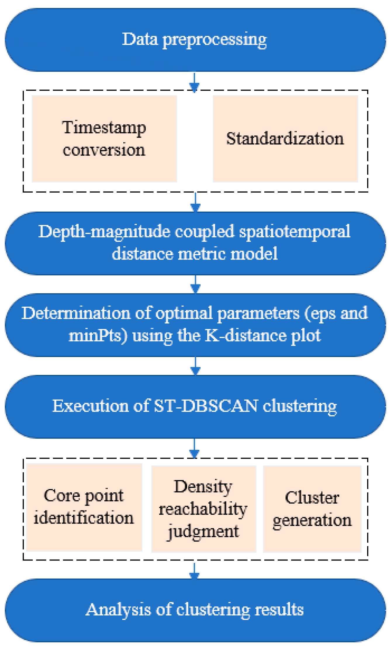
- Data Preprocessing
- a.
- Time-Feature Engineering
- b.
- Standardization
- (2)
- Depth–Magnitude Coupled Weighted Spatiotemporal Distance
- (3)
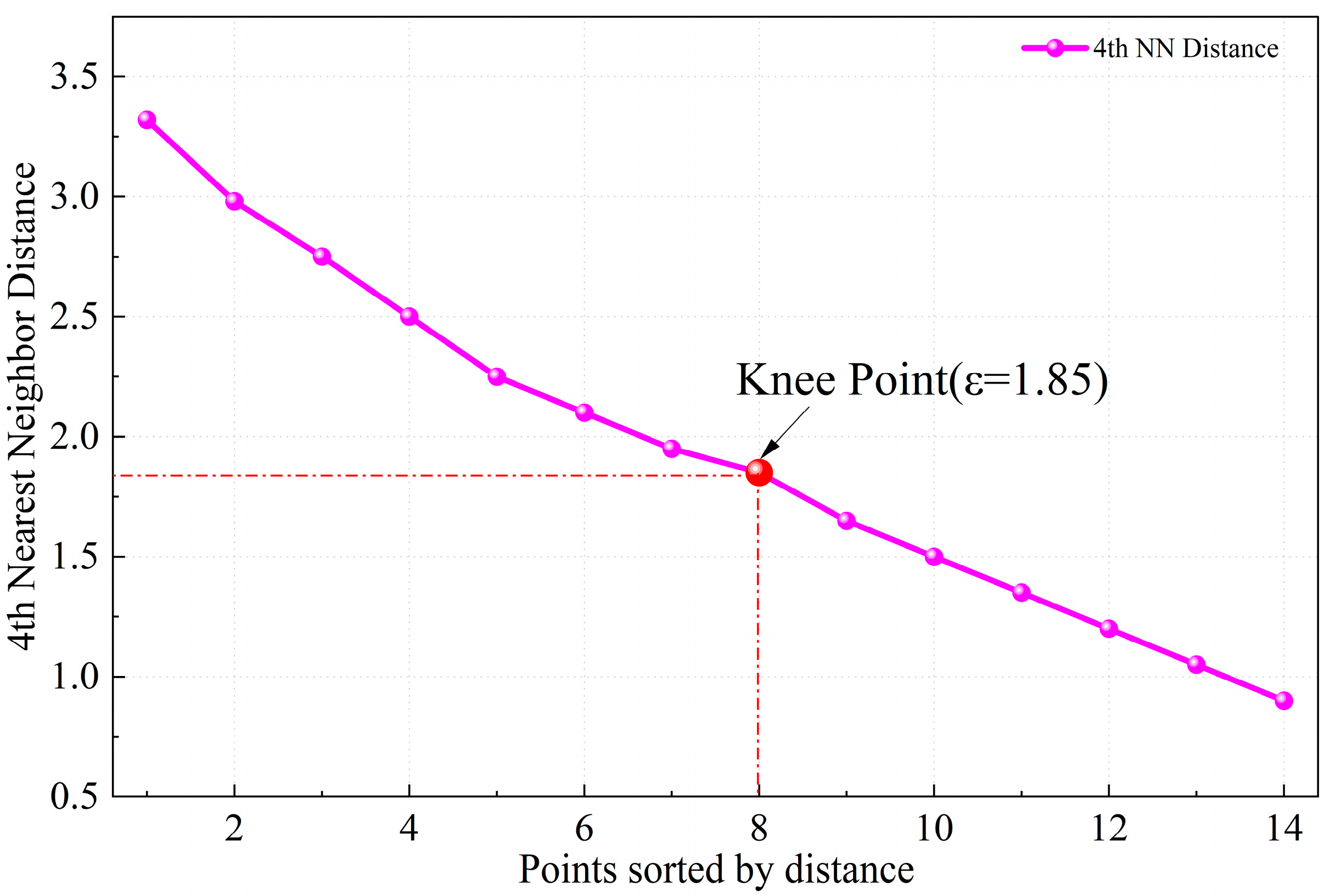
- ST-DBSCAN Parameter Setting
- (4)
- ST-DBSCAN Clustering Process
- (5)
- Clustering Result Analysis
2.3. Analysis Comparing ST-DBSCAN with Other Models
- (1)
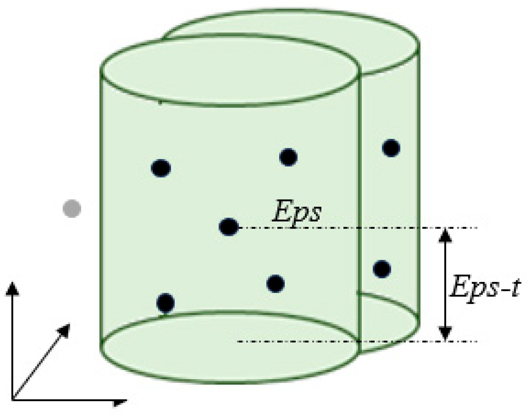
- ST-DBSCAN vs. OPTICS: ST-DBSCAN uses fixed spatiotemporal thresholds (Eps, t), while OPTICS generates a reachability plot to handle variable-density clusters.
- (2)
- ST-DBSCAN vs. HDBSCAN: HDBSCAN automates cluster selection via hierarchy and density stability, reducing noise sensitivity. ST-DBSCAN relies on manual eps/minPts tuning (via K-distance plots).
3. Case Study
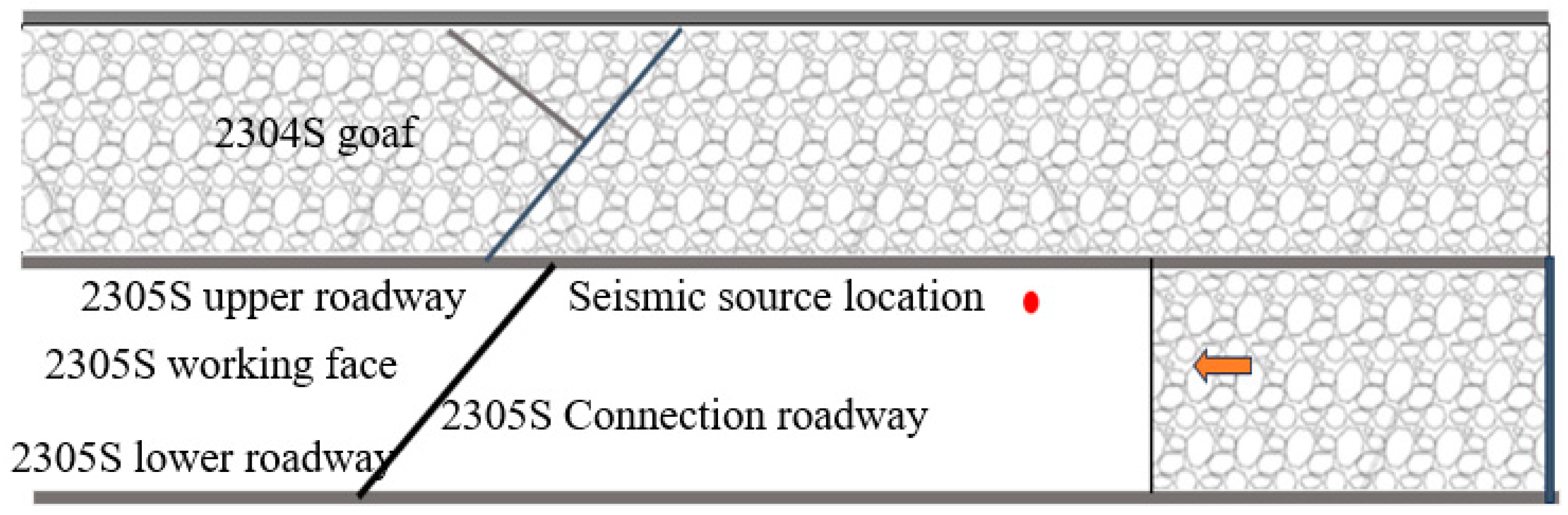
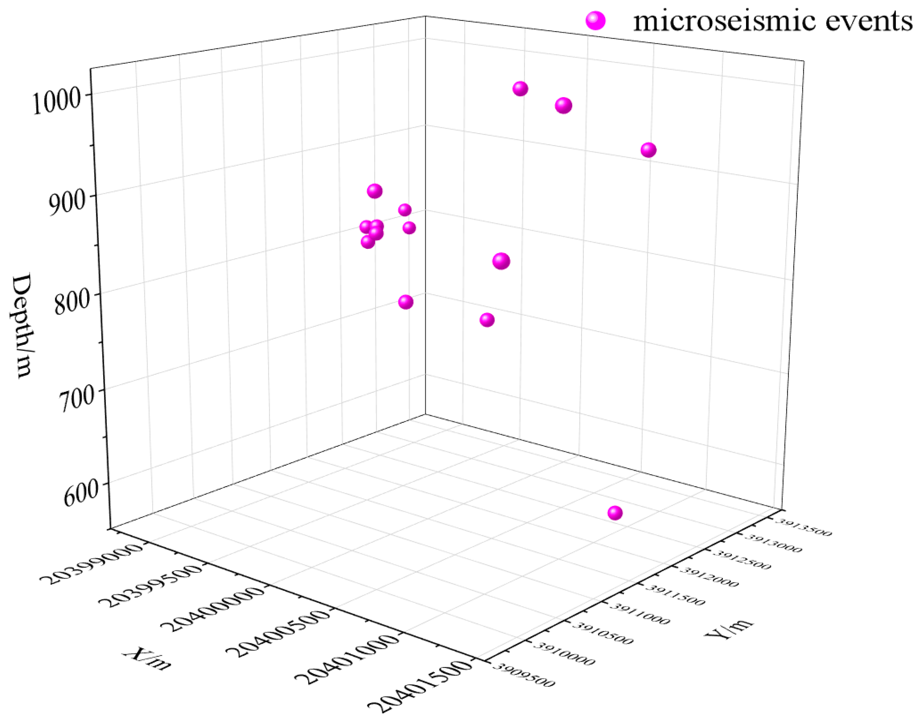
3.1. Event Background
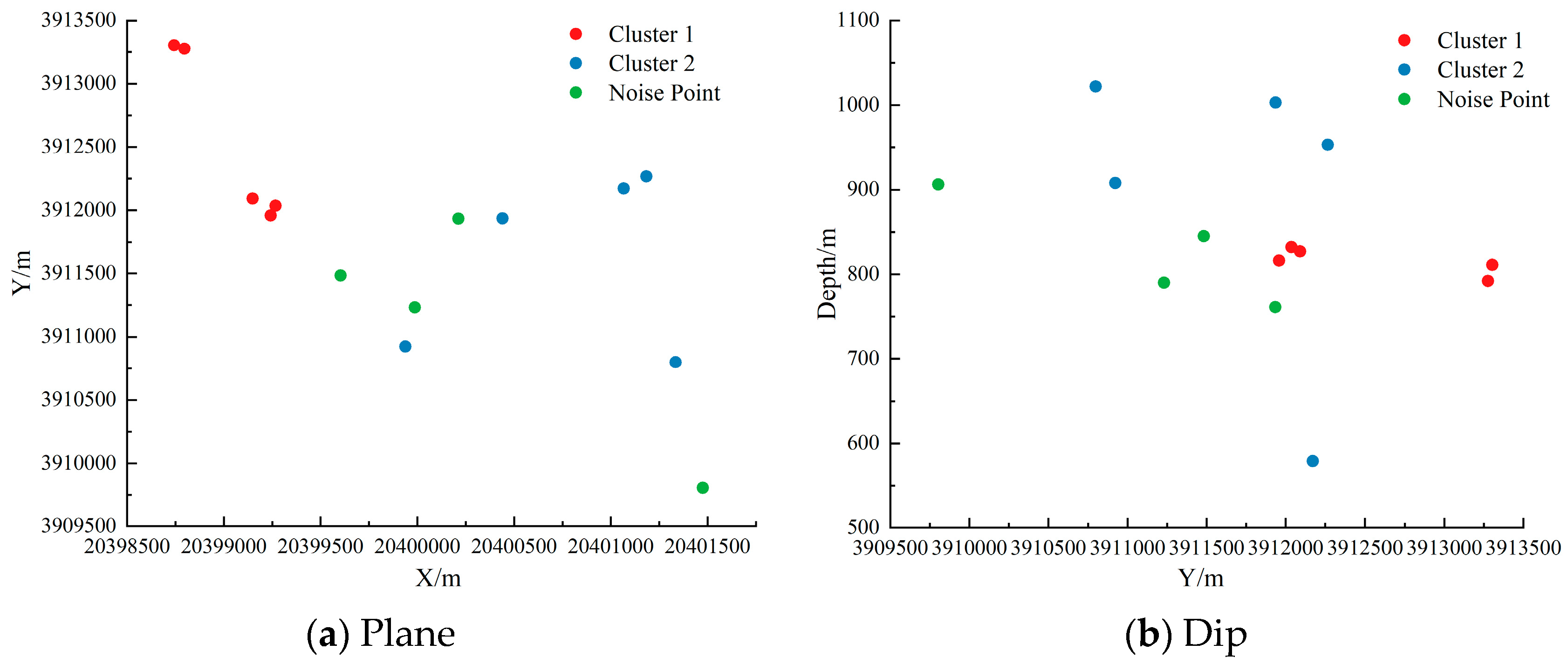
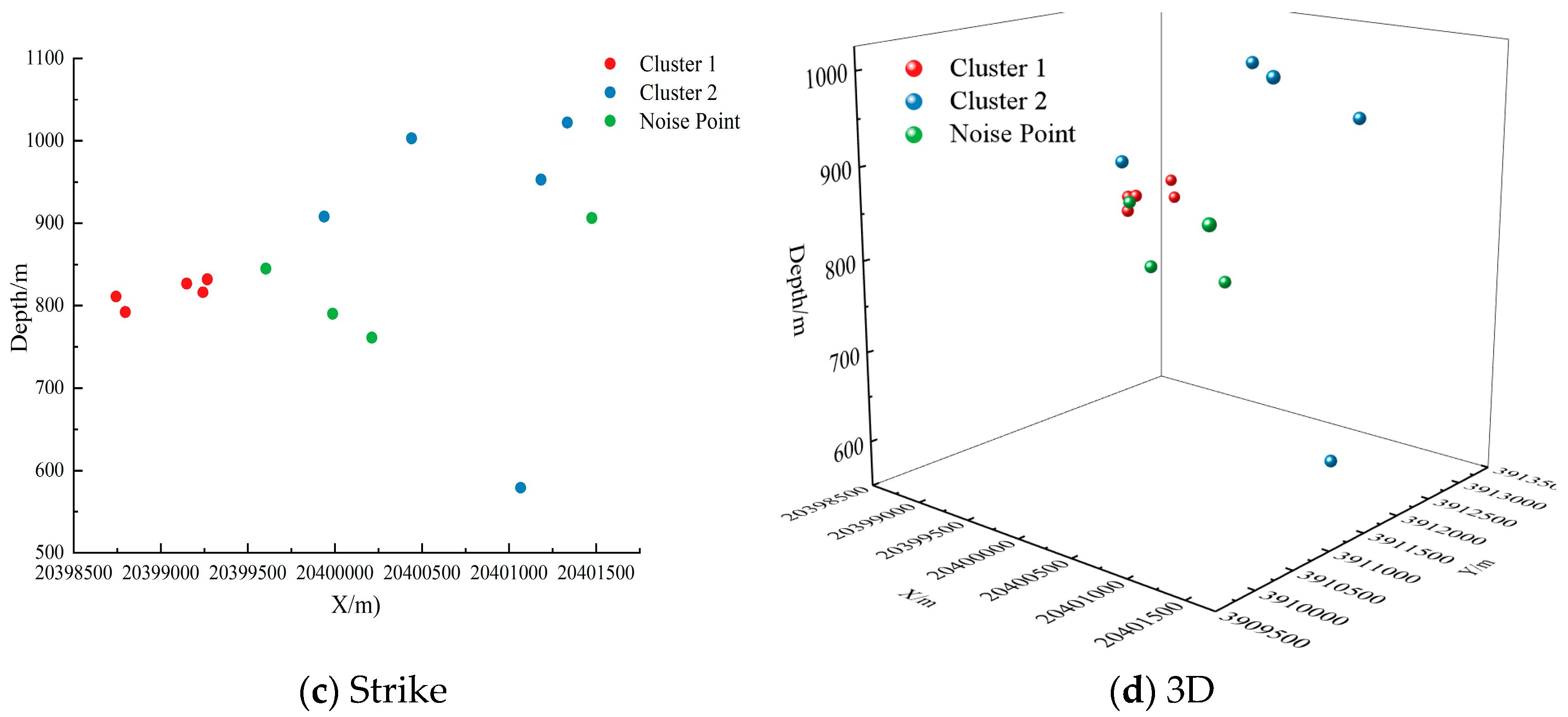
3.2. ST-DBSCAN Clustering Results
3.3. Design of the Comparative Experiment
4. Discussion
- (1)
- Calculations:
- (2)
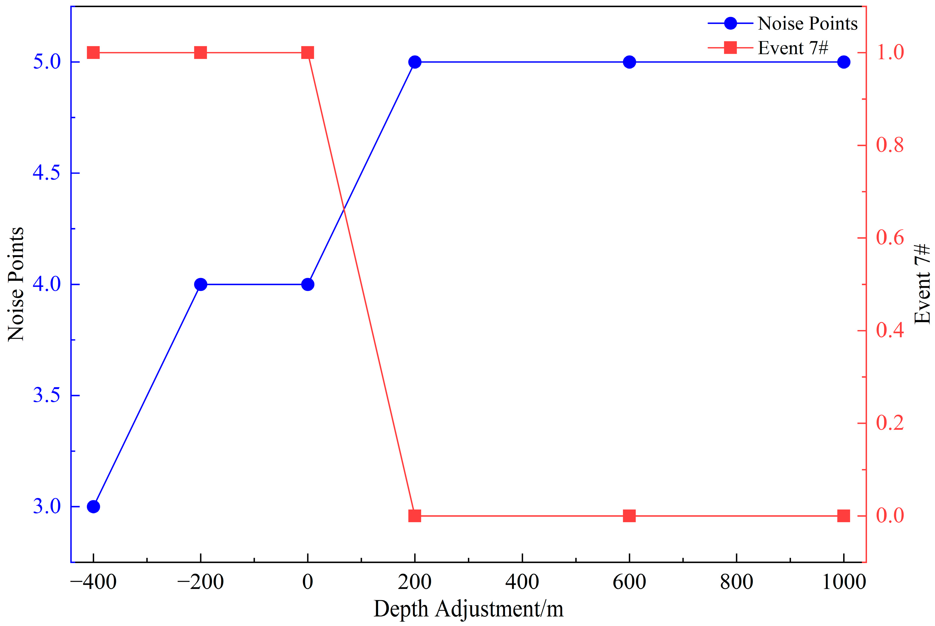
- Mining Depth Sensitivity Analysis:
- (3)
- Comparison with Actual Disaster Data
5. Conclusions
- (1)
- The core innovation of our ST-DBSCAN-based spatiotemporal analysis method for deep-mining microseismic data lies in its novel spatiotemporal clustering framework. This framework explicitly integrates both the temporal occurrence and spatial location attributes of microseismic events into a unified distance metric, effectively addressing the inherent limitations of traditional clustering algorithms (like DBSCAN), which typically handle spatial and temporal dimensions separately or inadequately. This integration directly leads to a significant enhancement in accurately identifying the complex spatiotemporal distribution patterns inherent in microseismic sequences.
- (2)
- Key to this method’s precision is the development of a tailored spatiotemporal distance metric model and the systematic optimization of spatiotemporal neighborhood parameters (Eps1 for space, and Eps2 for time), enabling the algorithm to discriminate and isolate distinct microseismic event clusters exhibiting diverse spatiotemporal characteristics (e.g., rapid bursts vs. prolonged swarms). Consequently, this method robustly delineates critical patterns such as temporal periodicity (e.g., shifts correlating with mining cycles or blasting schedules), spatial agglomeration zones (highlighting high-risk rock mass areas), and the dynamic spatiotemporal evolution and interaction pathways between these clusters over the monitoring period.
- (3)
- The analysis results in relation to actual deep-mining microseismic monitoring data show that different microseismic event clusters correspond to different rock mass failure processes and mining activity impacts, providing an important basis for comprehensively understanding the mechanical behavior of rock masses and disaster incubation mechanisms during deep mining.
- (4)
- To effectively monitor microseismic activities in longwall mining panels, we recommend adopting the following sensor layout strategy: “3D stereoscopic + key area densification”. In addition, the sensor layout should be dynamically adjusted in line with mining progress so as to realize real-time tracking of microseismic activities and early prediction of disasters, ensuring safe and efficient operations in longwall mining.
Author Contributions
Funding
Data Availability Statement
Conflicts of Interest
References
- Wang, S.; Liu, L.; Zhu, M.; Shen, Y.; Shi, Q.; Sun, Q.; Fang, Z.; Ruan, S.; He, W.; Yang, P.; et al. New way for green and low-carbon development of coal under the target of “double carbon”. J. China Coal Soc. 2024, 49, 152–171. [Google Scholar] [CrossRef]
- Yu, J.; Li, Z.; Yang, D.; Liu, Y.; Fang, S. Experimental study on dynamic evolutions of airflow in the ventilation network under the effect of mine gas outburst disasters. Sci. Rep. 2025, 15, 10651. [Google Scholar] [CrossRef] [PubMed]
- Yu, J.; Li, Z.; Yang, D.; Liu, Y. Dynamic Risk Assessment of Gas Accumulation During Coal and Gas Outburst Catastrophes Based on Analytic Hierarchy Process and Information Entropy. Processes 2025, 13, 1305. [Google Scholar] [CrossRef]
- Yuan, L.; Wang, E.Y.; Ma, Y.K.; Liu, Y.; Li, X. Research progress of coal and rock dynamic disasters and scientific and technological problems in China. J. China Coal Soc. 2023, 48, 1825–1845. [Google Scholar] [CrossRef]
- Yang, K.; Guo, P.H.; Yuan, L.; Cao, A.Y.; Zhang, Y.J.; Ma, Y.K.; Li, J.Z. Research progress on the conditions and mechanisms of typical dynamic disasters formation in deep coal mining. J. China Coal Soc. 2024, 50, 3352–3373. [Google Scholar] [CrossRef]
- Zhang, G.R.; Wang, E.Y.; Zhang, C.L.; Li, Z.H.; Wang, D.M. A Comprehensive Risk Assessment Method for Coal and Gas Outburst in Underground Coal Mines Based on Variable Weight Theory and Uncertainty Analysis. Process Saf. Environ. Prot. 2022, 167, 97–111. [Google Scholar] [CrossRef]
- Zhang, G.R.; Wang, E.; Liu, X.; Li, Z. Research on Risk Assessment of Coal and Gas Outburst During Continuous Excavation Cycle of Coal Mine with Dynamic Probabilistic Inference. Process Saf. Environ. Prot. 2024, 190, 405–419. [Google Scholar] [CrossRef]
- Fang, S.; Yin, S.; Li, Z.; Yang, D.; Wang, D.; Ding, Z.; Li, G. Study on the adsorption characteristics and pore-fissure response mechanism of meagre coal and anthracite under different methane pressures. Energy 2025, 332, 137283. [Google Scholar] [CrossRef]
- Cheng, J.; Song, G.; Sun, X.; Wen, L.; Li, F. Research developments and prospects on microseismic source location in mines. Engineering 2018, 4, 653–660. [Google Scholar] [CrossRef]
- Kinscher, J.; Bernard, P.; Contrucci, I.; Mangeney, A.; Piguet, J.P.; Bigarre, P. Location of microseismic swarms induced by salt solution mining. Geophys. J. Int. 2015, 200, 337–362. [Google Scholar] [CrossRef]
- Dou, L.M.; Cao, J.R.; Cao, A.Y.; Chai, Y.J.; Bai, J.Z.; Kan, J.L. Study on the types of coal mine seismicity and the propagation law of seismic waves. Coal Sci. Technol. 2021, 49, 23–31. [Google Scholar] [CrossRef]
- Zhu, G.A.; Jiang, Q.P.; Wu, Y.P.; Dou, L.M.; Lin, Z.Q.; Liu, H.Y. Numerical inversion of fault slip instability under stress wave disturbance. J. Min. Saf. Eng. 2021, 38, 370–379. [Google Scholar] [CrossRef]
- Song, D.Z.; He, X.Q.; Dou, L.M.; Zu, Z.Y.; Wang, A.H.; Li, Z.L. Research on detection technology of microseismic area with coal seam outburst risk. China Saf. Sci. J. 2021, 31, 89–94. [Google Scholar] [CrossRef]
- Cai, W.; Dou, L.M.; Wang, G.F.; Hu, Y.W. Mechanical mechanism of fault activation caused by coal seam mining activities and its induced rockburst mechanism. J. Min. Saf. Eng. 2019, 36, 1193–1202. [Google Scholar] [CrossRef]
- Zhu, G.A.; Jiang, Q.P.; Wu, Y.P.; Dou, L.M.; Xie, J.H.; Wang, C.; Liu, H.Y. Determination of reasonable final mining line position in deep working face based on “stress field-seismic wave field”. J. China Coal Soc. 2020, 45 (Suppl. S2), 571–580. [Google Scholar] [CrossRef]
- Huang, Q.G.; Gao, F. Application of Microseismic Monitoring Technology on Fully Mechanized Top-coal Caving Face of Extra-thick Coal Seam. In Proceedings of the 2011 International Conference on Multimedia Technology, Hangzhou, China, 26–28 July 2011. [Google Scholar] [CrossRef]
- Zhang, C.; Jin, G.H.; Liu, C.; Li, S.G.; Xue, J.H.; Cheng, R.H.; Wang, X.L.; Zeng, X.Z. Prediction of Rockbursts in A Typical Island Working Face of A Coal Mine Through Microseismic Monitoring Technology. Tunn. Undergr. Space Technol. 2021, 110, 103827. [Google Scholar] [CrossRef]
- Cai, W.; Dou, L.M.; Zhang, M.; Chen, W.Z.; Shi, J.Q.; Fan, L.F. A Fuzzy Comprehensive Evaluation Methodology for Rock Burst Forecasting Using Microseismic Monitoring. Tunn. Undergr. Space Technol. 2018, 80, 232–245. [Google Scholar] [CrossRef]
- Cai, W.; Dou, L.M.; Si, G.Y.; Cao, A.Y.; Gong, S.Y.; Wang, G.F.; Yuan, S.S. A New Seismic-Based Strain Energy Methodology for Coal Burst Forecasting in Underground Coal Mines. Int. J. Rock Mech. Min. Sci. 2019, 123, 104086. [Google Scholar] [CrossRef]
- Shi, F.; Zhang, D.; Wang, P.; Cai, Y.; Yuan, B. Investigation on Rock Mass Stability Monitoring System and Activity Characteristic in Deep Mining. MATEC Web Conf. 2022, 356, 01009. [Google Scholar] [CrossRef]
- Dong, L.J.; Tang, Z.; Li, X.B.; Chen, Y.C.; Xue, J.C. Discrimination of mining microseismic events and blasts using convolutional neural networks and original waveform. J. Cent. South Univ. Technol. 2020, 27, 3078–3089. [Google Scholar] [CrossRef]
- Cao, A.Y.; Yang, X.; Wang, C.B.; Li, S.; Liu, Y.Q. High-precision phase picking and automatic source locating method for seismicity in mines based on deep transfer learning. J. China Coal Soc. 2023, 48, 4393–4405. [Google Scholar] [CrossRef]
- Yang, X.; Li, Y.P.; Cao, A.Y.; Li, Y.Q.; Wang, C.B.; Zhang, W.W.; Niu, Q. Coal Burst Spatio-Temporal Prediction Method Based on Bidirectional Long Short-Term Memory Network. Int. J. Coal Sci. Technol. 2025, 12, 11. [Google Scholar] [CrossRef]
- Song, J.F.; Li, C.P.; Zhang, X.F.; Sun, C.H.; Zhang, J.; Zhang, Z.G. Application of Bayesian Method for Mining-Induced Tremors: A Case Study of the Xinjulong Coal Mine in China. Int. J. Rock Mech. Min. Sci. 2024, 174, 105642. [Google Scholar] [CrossRef]
- Ester, M.; Kriegel, H.P.; Sander, J.; Xu, X. A density-based algorithm for discovering clusters in large spatial databases with noise. In Proceedings of the 2nd International Conference on Knowledge Discovery and Data Mining (KDD’96), Portland, OR, USA, 2–4 August 1996; pp. 226–231. [Google Scholar] [CrossRef]
- Zhang, X.; Chen, Y.; Jia, J.; Kuang, K.; Lan, Y.; Wu, C. Multi-view density-based field-road classification for agricultural machinery: DBSCAN and object detection. Comput. Electron. Agric. 2022, 200, 107263. [Google Scholar] [CrossRef]
- Zhang, G.H. Analysis of spatio-temporal characteristics of mine rock burst microseismic monitoring data based on ST-DBSCAN clustering algorithm. China Energy Environ. Prot. 2024, 46, 62–70. [Google Scholar] [CrossRef]
- Li, Y. Research on Vessel Behavior Recognition Method Based on Spatial-Temporal Movement Features. Master’s Thesis, Dalian Maritime University, Dalian, China, 2024. [Google Scholar]
- Rong, H.; Wei, S.L.; Zhang, H.W.; Chen, L.; Li, N. Influencing factors and distribution characteristics of rock burst under complex geological dynamic environment. Coal Sci. Technol. 2025, 53, 423–434. [Google Scholar]
- Rizvi, Z.H.; Mustafa, S.H.; Sattari, A.S.; Ahmad, S.; Furtner, P.; Wuttke, F. Dynamic Lattice Element Modelling of Cemented Geomaterials. In Advances in Computer Methods and Geomechanics; Prashant, A., Sachan, A., Desai, C., Eds.; Lecture Notes in Civil Engineering; Springer: Singapore, 2020; Volume 55, pp. 689–701. [Google Scholar] [CrossRef]
- Ahmad, S.; Ahmad, S.; Akhtar, S.; Rizvi, Z.H.; Wuttke, F. Data-driven assessment of corrosion in reinforced concrete structures embedded in clay dominated soils. Sci. Rep. 2025, 15, 22744. [Google Scholar] [CrossRef] [PubMed]
- Ahmad, S.; Rizvi, Z.H.; Arp, J.C.C.; Wuttke, F.; Tirth, V.; Islam, S. Evolution of Temperature Field around Underground Power Cable for Static and Cyclic Heating. Energies 2021, 14, 8191. [Google Scholar] [CrossRef]
- Ahmad, S.; Rizvi, Z.H.; Wuttke, F. Unveiling soil thermal behavior under ultra-high voltage power cable operations. Sci. Rep. 2025, 15, 7315. [Google Scholar] [CrossRef] [PubMed]
- Ahmad, S.; Rizvi, Z.H.; Khan, M.A.; Ahmad, J.; Wuttke, F. Experimental study of thermal performance of the backfill material around underground power cable under steady and cyclic thermal loading. Mater. Today Proc. 2019, 17, 85–95. [Google Scholar] [CrossRef]

| Dimension | DBSCAN | ST—DBSCAN |
|---|---|---|
| Data Type | Purely spatial data (such as coordinate points) | Spatiotemporal data (space + timestamp) |
| Neighborhood Definition | Only spatial distance ε | Spatial distance εs + time difference εt |
| Cluster Characteristics | Spatial density-connected | Spatio-temporally density-connected (both space and time are adjacent) |
| Typical Applications | Spatial clustering (such as user location distribution) | Spatio-temporal pattern analysis (such as disaster event chains) |
| No. | Date | X/m | Y/m | Depth/m | Energy/J | Location | Magnitude (Approximate) |
|---|---|---|---|---|---|---|---|
| 1# | 22 February 2020 6:17:22 | 20,399,987 | 3,911,232 | 790 | 4.25 × 10⁷ | 2305S working face (960 m) | 1.22 |
| 2# | 28 February 2020 12:43:56 | 20,401,067 | 3,912,171 | 579 | 4.22 × 10⁵ | 8303 working face (950 m) | 0.55 |
| 3# | 12 March 2021 16:33:09 | 20,399,938 | 3,910,924 | 908 | 2.57 × 10⁵ | 2304 goaf (950 m) | 0.47 |
| 4# | 9 April 2021 22:49:52 | 20,400,440 | 3,911,937 | 1003 | 2.34 × 10⁵ | 2306 lower roadway (1030 m) | 0.44 |
| 5# | 23 May 2021 13:25:01 | 20,399,242 | 3,911,958 | 816 | 6.12 × 10⁴ | Near 6304 goaf (860 m) | 0.06 |
| 6# | 21 June 2021 10:19:22 | 20,399,268 | 3,912,036 | 832 | 2.22 × 10⁴ | 6304 goaf (840 m) | −0.23 |
| 7# | 7 July 2021 0:20:34 | 20,398,797 | 3,913,277 | 792 | 1.69 × 10⁴ | 6305 working face (800 m) | −0.38 |
| 8# | 7 July 2021 22:10:43 | 20,399,149 | 3,912,091 | 827 | 1.68 × 10⁴ | 6304 working face (840 m) | −0.38 |
| 9# | 15 July 2021 10:54:07 | 20,401,335 | 3,910,800 | 1022 | 1.66 × 10⁴ | 2308 working face (920 m) | −0.39 |
| 10# | 22 July 2021 19:32:44 | 20,398,743 | 3,913,303 | 811 | 1.40 × 10⁴ | 6304 lower roadway (790 m) | −0.49 |
| 11# | 24 July 2021 12:11:22 | 20,401,475 | 3,909,804 | 906 | 1.34 × 10⁴ | 2307 working face (860 m) | −0.48 |
| 12# | 1 August 2021 14:17:22 | 20,401,184 | 3,912,266 | 953 | 1.30 × 10⁴ | 8303 working face (970 m) | −0.45 |
| 13# | 2 August 2021 9:32:49 | 20,399,603 | 3,911,483 | 845 | 1.14 × 10⁴ | Near 2303 working face (890 m) | −0.49 |
| 14# | 25 October 2021 6:45:17 | 20,400,212 | 3,911,934 | 761 | 2.61 × 10⁷ | Near ventilation roadway of north district (990 m) | 1.41 |
| No. | Time | Unix Timestamp (Seconds) | No. | Time | Unix Timestamp (Seconds) |
|---|---|---|---|---|---|
| 1# | 22 February 2020 6:17:22 | 1,582,347,442 | 8# | 7 July 2021 22:10:43 | 1,625,688,243 |
| 2# | 28 February 2020 12:43:56 | 1,582,903,436 | 9# | 15 July 2021 10:54:07 | 1,626,341,647 |
| 3# | 12 March 2021 16:33:09 | 1,615,566,789 | 10# | 22 July 2021 19:32:44 | 1,626,982,364 |
| 4# | 9 April 2021 22:49:52 | 1,618,003,792 | 11# | 24 July 2021 12:11:22 | 1,626,908,482 |
| 5# | 23 May 2021 13:25:01 | 1,621,776,301 | 12# | 1 August 2021 14:17:22 | 1,627,817,842 |
| 6# | 21 June 2021 10:19:22 | 1,624,275,562 | 13# | 2 August 2021 9:32:49 | 1,627,904,569 |
| 7# | 7 July 2021 0:20:34 | 1,625,607,634 | 14# | 25 October 2021 6:45:17 | 1,635,125,117 |
| Column Name(s) | Mean | Std |
|---|---|---|
| X/m | 20,400,038.50 | 994.34 |
| Y/m | 3,911,746.50 | 885.56 |
| Depth/m | 858.00 | 130.38 |
| Energy/J | 3.34 × 10⁶ (3,340,000) | 1.13 × 10⁷ (11,300,000) |
| Magnitude | −0.03 | 0.69 |
| Unix (seconds) | 1,620,409,330.21 | 19,485,439.34 |
| No. | X Scaled/m | Y Scaled/m | Depth Scaled/m | Energy Scaled/J | Magnitude Scaled | Unix Scaled/s |
| 1# | 1.96 | −0.74 | −0.52 | 3.46 | 1.81 | −1.95 |
| 2# | 1.04 | 0.05 | −2.14 | 0.03 | 0.84 | −1.92 |
| 3# | 2.06 | −0.93 | 0.39 | −0.07 | 0.72 | −0.23 |
| 4# | 0.40 | 0.02 | 1.11 | −0.09 | 0.67 | 0.09 |
| 5# | −0.84 | 0.02 | −0.32 | −0.24 | 0.04 | 0.59 |
| 6# | −0.81 | 0.08 | −0.20 | −0.27 | −0.25 | 1.23 |
| 7# | −1.25 | 1.75 | −0.50 | −0.28 | −0.51 | 1.80 |
| 8# | −0.90 | 0.16 | −0.24 | −0.28 | −0.51 | 1.85 |
| 9# | 1.30 | −1.09 | 1.26 | −0.28 | −0.52 | 1.95 |
| 10# | −1.31 | 1.79 | −0.36 | −0.28 | −0.67 | 2.08 |
| 11# | 1.44 | −2.12 | 0.37 | −0.29 | −0.65 | 2.04 |
| 12# | 1.09 | 0.09 | 0.73 | −0.29 | −0.61 | 2.13 |
| 13# | −0.45 | −0.37 | −0.10 | −0.28 | −0.67 | 2.14 |
| 14# | 0.17 | 0.02 | −0.75 | 2.01 | 2.09 | 5.90 |
| No. | X/m | Y/m | Depth/m | Magnitude | Cluster | Spatiotemporal Characteristic Analysis |
|---|---|---|---|---|---|---|
| #1 | 20,399,987 | 3,911,232 | 790 | 1.22 | −1 | High magnitude, spatiotemporal isolation (edge region) |
| #2 | 20,401,067 | 3,912,171 | 579 | 0.55 | 2 | Core cluster, shallow low-energy disturbance |
| #3 | 20,399,938 | 3,910,924 | 908 | 0.47 | 2 | Core cluster, deep-mining activities |
| #4 | 20,400,440 | 3,911,937 | 1003 | 0.44 | 2 | Core cluster, deep-mining activities |
| #5 | 20,399,242 | 3,911,958 | 816 | 0.06 | 1 | Core cluster, middle-layer mining disturbance |
| #6 | 20,399,268 | 3,912,036 | 832 | −0.23 | 1 | Core cluster, middle-layer mining disturbance |
| #7 | 20,398,797 | 3,913,277 | 792 | −0.38 | 1 | Core cluster, middle-layer mining disturbance |
| #8 | 20,399,149 | 3,912,091 | 827 | −0.38 | 1 | Core cluster, middle-layer mining disturbance |
| #9 | 20,401,335 | 3,910,800 | 1022 | −0.39 | 2 | Core cluster, deep-mining activities |
| #10 | 20,398,743 | 3,913,303 | 811 | −0.49 | 1 | Core cluster, middle-layer mining disturbance |
| #11 | 20,401,475 | 3,909,804 | 906 | −0.48 | −1 | Core cluster, middle-layer mining disturbance |
| #12 | 20,401,184 | 3,912,266 | 953 | −0.45 | 2 | Core cluster, deep-mining activities |
| #13 | 20,399,603 | 3,911,483 | 845 | −0.49 | −1 | Core cluster, middle-layer mining disturbance |
| #14 | 20,400,212 | 3,911,934 | 761 | 1.41 | −1 | High magnitude, spatiotemporal isolation (edge region) |
| Algorithm | Silhouette | DB Index | Noise Detection | Interpretability |
|---|---|---|---|---|
| ST-DBSCAN | 0.62 | 0.81 | 100% (4/4) | Provides clear core/abnormal separation |
| DBSCAN | 0.41 | 1.32 | 50% (2/4) | Ignores time and merges async events |
| K-means | 0.38 | 1.45 | 25% (1/4) | Fails to detect noise (fixed k = 3) |
| OPTICS | 0.55 | 0.95 | 75% (3/4) | Is sensitive to time windows and allows complex parameter tuning |
| Depth Adjustment | Cluster | Noise Point |
|---|---|---|
| Original(0) | [5, 6, 7, 8, 10], [2, 3, 4, 9, 12] | [1, 11, 13, 14] |
| −400 | [5, 6, 7, 8, 10], [2, 3, 4, 9, 11, 12] | [1, 13, 14] |
| −200 | [5, 6, 7, 8, 10], [2, 3, 4, 9, 12] | [1, 11, 13, 14] |
| +200 | [5, 6, 8, 10], [2, 3, 4, 9, 12] | [1, 7, 11, 13, 14] |
| +600 | [5, 6, 8, 10], [2, 3, 4, 9, 12] | [1, 7, 11, 13, 14] |
| +1000 | [5, 6, 8, 10], [2, 3, 4, 9, 12] | [1, 7, 11, 13, 14] |
Disclaimer/Publisher’s Note: The statements, opinions and data contained in all publications are solely those of the individual author(s) and contributor(s) and not of MDPI and/or the editor(s). MDPI and/or the editor(s) disclaim responsibility for any injury to people or property resulting from any ideas, methods, instructions or products referred to in the content. |
© 2025 by the authors. Licensee MDPI, Basel, Switzerland. This article is an open access article distributed under the terms and conditions of the Creative Commons Attribution (CC BY) license (https://creativecommons.org/licenses/by/4.0/).
Share and Cite
Yu, J.; He, H.; Liu, Z.; He, X.; Zhou, F.; Song, Z.; Yang, D. Analysis of Spatiotemporal Characteristics of Microseismic Monitoring Data in Deep Mining Based on ST-DBSCAN Clustering Algorithm. Processes 2025, 13, 2359. https://doi.org/10.3390/pr13082359
Yu J, He H, Liu Z, He X, Zhou F, Song Z, Yang D. Analysis of Spatiotemporal Characteristics of Microseismic Monitoring Data in Deep Mining Based on ST-DBSCAN Clustering Algorithm. Processes. 2025; 13(8):2359. https://doi.org/10.3390/pr13082359
Chicago/Turabian StyleYu, Jingxiao, Hongsen He, Zongquan Liu, Xinzhe He, Fengwei Zhou, Zhihao Song, and Dingding Yang. 2025. "Analysis of Spatiotemporal Characteristics of Microseismic Monitoring Data in Deep Mining Based on ST-DBSCAN Clustering Algorithm" Processes 13, no. 8: 2359. https://doi.org/10.3390/pr13082359
APA StyleYu, J., He, H., Liu, Z., He, X., Zhou, F., Song, Z., & Yang, D. (2025). Analysis of Spatiotemporal Characteristics of Microseismic Monitoring Data in Deep Mining Based on ST-DBSCAN Clustering Algorithm. Processes, 13(8), 2359. https://doi.org/10.3390/pr13082359