Abstract
Effective inventory management in decentralized multi-echelon supply chains (MESCs) is essential for minimizing costs and improving service levels. This study introduces a two-stage approach that combines discrete-event simulation and multi-variate regression analysis (MVRA) to analyze a three-echelon supply chain. The first stage simulates various inventory policies and demand scenarios across manufacturers, wholesalers, and retailers. The second stage uses MVRA to examine how inventory decisions at each echelon influence key performance indicators, including inventory cost and inventory level. The results identify the parameters that most significantly affect supply chain performance, offering practical guidance for optimizing policies in complex and decentralized systems.
1. Introduction
Controlling the flow of goods within a supply chain can significantly impact enterprise competitiveness in today’s globalized environment, where information flows quickly. A Multi-Echelon Supply Chain (MESC) network consists of stages through which materials move from raw material sources to final consumers. A typical three-echelon supply network comprises suppliers, manufacturers, and retailers, where materials are transformed in shape, count, and size as they progress through the chain. At each echelon or node, key decisions must be made regarding replenishment quantities, ordering frequency, demand fulfillment, and service levels. Although holding inventory is necessary to accommodate random fluctuations and emergencies, it also ties up working capital. Therefore, inventory control and coordination across nodes are crucial for improving the overall supply chain performance.
Inventory drivers contributing to the stochastic nature of supply chains can be categorized into controllable decision variables, such as production strategy, production capacity, forecast accuracy, and replenishment policy, and uncontrollable inputs, such as patterns of lead times, supply and demand mean, and variability. Both types of drivers influence supply chain performance, which is primarily measured by supply chain cost and stockholding level. The key cost components include material, production, and holding costs at each echelon, stock-out costs, and transfer costs between echelons.
This study aims to analyze a decentralized MESC network using a two-stage approach: (1) simulating the MESC network to evaluate its performance, and (2) parameterizing inventory cost functions for each echelon using multi-variate regression analysis (MVRA). By applying MVRA, this research explores how inventory policies simultaneously respond to changes in inventory parameters and affect supply chain performance, as measured by inventory costs and average on-hand stock at each echelon.
Efficient inventory management in decentralized MESCs is a persistent and evolving challenge. In such systems, inventory decisions are made independently at each echelon (e.g., manufacturer, wholesaler, retailer), often leading to suboptimal global performance due to a lack of coordination. These inefficiencies can result in excessive inventory costs, frequent stock-outs, and delayed responses to demand variabilities. With the growing complexity and uncertainty of global supply chains, understanding how local inventory policies affect system-wide behavior is increasingly critical.
Although many studies focus on centralized inventory systems, where unified decision-making enables global optimization, decentralized systems are more commonly used in practice. However, they have been studied less thoroughly due to their inherent complexity. Advances in discrete-event simulation (DES), machine learning, and stochastic optimization have created new opportunities for analyzing decentralized inventory behavior at scale. However, there is a need for integrated frameworks that combine simulation with data-driven analysis to evaluate how performance metrics respond to changes in inventory strategies.
This paper addresses this gap by developing a two-stage methodology. First, a discrete-event simulation model of a three-echelon decentralized supply chain is developed, incorporating typical inventory policies at each echelon under stochastic demand and lead-time conditions. Second, the simulation outputs are analyzed using multi-variate regression analysis (MVRA) to identify which inventory parameters most significantly influence costs and on-hand stock across the supply chain.
The novelty of this study lies in the integration of operational simulation with statistical regression analysis to systematically examine the interactions between local policies and global outcomes. The findings offer practical guidance to supply chain managers operating in decentralized environments, as well as a scalable methodology that can be extended to more complex multiproduct systems.
The main contributions of this study are as follows:
- It proposes a hybrid simulation-regression approach for inventory analysis in decentralized supply chains.
- It models a three-echelon structure with independent decision-making across tiers.
- It identifies the key policy parameters influencing cost and inventory behavior across echelons.
- It outlines a scalable framework that can be extended to complex multiproduct environments.
The remainder of this paper is organized as follows. Section 2 reviews the relevant literature on decentralized supply chains, inventory control, and simulation-based approaches. Section 3 outlines the research methodology, including the simulation model design and the regression framework. Section 4 presents the case study setup and input parameterizations. Section 5 details the multi-variate regression analysis and discusses the key findings in terms of cost and inventory behavior. Section 6 concludes the study by summarizing the key contributions, discussing the managerial implications, and suggesting directions for future research.
2. Literature Review
Coordination across echelons is critical for effective production planning and responsiveness to market demands [1]. This simulation-based approach demonstrates how echelon-level decisions significantly impact overall supply chain performance. Furthermore, as explained in [2], the stochastic characteristics of lead times across multiple echelons highlight the structural complexity inherent in MESCs. These variable lead times necessitate sophisticated forecasting and planning mechanisms to maintain service levels and reduce inefficiencies in the supply chain. This work was extended to structural analysis by applying control theory to model the dynamic behavior of MESCs, especially under disruption [3].
Inventory control in MESCs is increasingly challenged by uncertainties in demand, supply disruptions, and the need for technological adaptation. Recent studies have examined demand variability, bullwhip effect mitigation, and the use of artificial intelligence (AI) for improved forecasting and replenishment strategies. A key concern is that demand uncertainty and lead time variability amplify the bullwhip effect, which increases inventory oscillations across echelons. For instance, highlighted the stochastic nature of lead times as a critical factor in the bullwhip effect, particularly when these lead times are not accurately accounted for in the planning models. Reinforcement learning (RL) techniques have gained popularity to counteract these issues. A Proximal Policy Optimization (PPO2) algorithm was implemented to manage seasonal demand and variable lead times, showing improved performance over traditional linear methods [4]. Both model-based and model-free strategies in behaviorally grounded supply chain settings have been explored [5]. This dual approach addresses the psychological factors affecting ordering behaviors, providing a comprehensive toolset for inventory.
Variability in demand and lead times can destabilize inventory systems and increase costs. Empirical evidence shows that increased lead time variability correlates with higher inventory and operational costs, particularly impacting just-in-time systems [6]. Demand fluctuation is a primary source of uncertainty [7], where supply chain models with stochastic lead time demand impact profit and inventory strategies. Simulation modeling can show that increased demand variability deteriorates performance in terms of customer satisfaction, operational cost, and environmental impact [8]. A Vendor Managed Inventory (VMI) model, which is designed to handle uncertain demand in pharmaceutical supply chains, also reduces stockouts [9]. Feedback-based deterministic optimization for robust decision-making under demand uncertainty was introduced in [10]. Demand uncertainty is incorporated into designing a sustainable closed-loop pharmaceutical supply chain, emphasizing resilience and environmental performance [11].
Supply chain performance is a critical metric for evaluating the efficiency, responsiveness, and resilience of logistics networks. These performance outcomes are significantly influenced by various controllable and uncontrollable drivers. Strategic decisions regarding production methods and capacity constraints directly influence supply chain agility. Synchronizing capacity and production planning is important for meeting fluctuating demands [12]. Forecasting is a pivotal decision variable that underpins inventory and replenishment decisions. Machine learning significantly improves forecast accuracy in pharmaceutical supply chains, thereby increasing resilience and reducing errors [13]. Recent innovations—such as multi-agent reinforcement learning (MARL) and graph neural networks (GNNs)—have been deployed in decentralized inventory systems. Addressing dimensionality, decentralized decision-making, and optimizing inventory in complex multi-echelon systems is performed using a multi-agent DRL framework with GNNs [14]. A case study on fast-moving consumer goods (FMCG) demonstrated that improved forecast accuracy directly correlates with better inventory management and reduced costs [15]. Effective replenishment strategies mitigate stock-outs and reduce the carrying costs. The use of linear Min-Plus systems to design control laws for supply chains facing disruptions emphasized replenishment control under constraint conditions [16]. Holding and shortage costs are reduced by optimizing the periodic review joint replenishment policy to manage stochastic inventory systems [17]. MAP (Markovian Arrival Process) demand efficient models are analyzed by a hybrid replenishment policy combining continuous and periodic review mechanisms [18].
Simulation models are pivotal in handling the complexity of MESCs [14]. It is adapted to model perishable inventory in healthcare, highlighting the continued relevance and diversity of discrete-event simulation-based inventory studies. He (2024) [1] proposed a simulation-based coordination strategy for production planning across supply chain levels, enhancing efficiency and adaptability in dynamic environments. The impact of uncertain demands and lead times reinforces the need for robust and adaptable inventory strategies [19]. The impacts of simultaneous supply and demand disruptions on MESCs are quantitatively analyzed [20]. This paper emphasizes the importance of comprehensive planning and responsive strategies to mitigate risks and maintain operational stability. Simulation techniques have been applied to optimize sustainable agri-food supply chains, revealing the potential to align economic and environmental goals [21]. In the context of biofuel logistics, a comprehensive review of simulation paradigms—discrete-event, system dynamics, and agent-based simulations—demonstrating their application in improving ethanol supply chains, is provided in [22]. During the COVID-19 pandemic, AnyLogistix is used to simulate disruptions in medical mask supply chains and test resilience strategies, such as backup facilities [23].
Statistical methods are also widely used in supply chain research for decision-making under uncertainty, performance evaluation, and optimization. In particular, regression techniques are employed to examine the effects of strategic and operational decisions. Multiple regression analysis can be used to assess the impact of logistics postponement strategies on consumer perceptions in e-commerce [24]. COVID-19 indicators are linked to logistics efficiency via regression modeling [25]. Strong correlations exist when using linear regression to explore the economic-logistics linkages in major Chinese metropolitan areas, which underscores the role of logistics in economic development [26].
In summary, the literature illustrates the complexity of managing decentralized MESCs, especially under demand variability, lead time uncertainty, and disruptions. Prior research emphasizes the value of echelon coordination, simulation and AI tools, and statistical methods like regression, for performance modeling. However, a gap remains in understanding how inventory parameters influence performance in decentralized systems, where decisions are made independently. This study addresses this gap by integrating simulation and multi-variate regression analysis to evaluate the sensitivity of performance metrics to inventory decisions across echelons. The proposed framework supports better policy evaluation in decentralized environments, fostering more informed, data-driven supply chain planning.
3. MESC Model Description
This study examines a three-echelon, multi-period, decentralized supply chain with a single manufacturer (M), wholesaler (W), and retailer (R), where the supply of raw materials to the manufacturer is assumed to be uninterrupted. The model assumes:
- A single product flows from a raw material supplier to an end consumer
- Random customer demand occurs at the retailer level
- Inventory quantities are integer-valued across all echelons
- Holding costs are linear and time-based
- Shortages are permitted and are associated with specific penalty costs
- Unfilled demand results in lost sales at the retailer, but backorders at the manufacturer and wholesaler
- Transportation costs are calculated per shipment
- Manufacturing costs are proportional to production volume
- All echelons operate under finite capacity constraints
Different inventory replenishment policies are applied at each echelon:
- Manufacturer’s raw material inventory (Min): Continuous review (s, Q) policy
- Manufacturer’s finished product inventory (Mout): Continuous review (s, S) policy
- Wholesaler: Periodic review (R, S) policy
- Retailer: Continuous review (s, Q) policy
Supply chain costs include those incurred from holding inventory at each echelon, chances of shortages, transfer of items between echelons, and material and manufacturing costs. Holding costs are determined by the inventory on hand and unit-carrying costs. Shortage costs are calculated for each occurrence. Shortages occur when demand is unmet. Unfilled demand at the retailer leads to lost sales. In this case, the loss of benefit, customer, and goodwill determines the shortage cost of the lost unfilled demand. At the manufacturer and wholesaler, unmet demand is backordered. A penalty is applied for each unfilled order.
We built a simulation model to evaluate the supply chain performance under varying inventory parameters. The key aspects of the experiment are as follows:
- 3200 scenarios with different input settings
- Each scenario runs for 5000 h
- Tracked outputs include cost components and average on-hand inventory at each echelon
- Input parameters include replenishment policy parameters, lead times, and demand patterns
3.1. Model Notations
The following notation is used as input to the simulation to calculate the supply chain costs:
| Reorder level of raw material at manufacturer | |
| Replenishment order quantity of raw material at manufacturer | |
| Reorder level of finished products at manufacturer | |
| Order-up-to level of finished products at manufacturer | |
| Review time interval at wholesaler | |
| Order-up-to level at wholesaler | |
| Reorder level at retailer | |
| Replenishment order quantity at retailer | |
| Distribution of customer demand transaction | |
| Distribution of time between customer demand | |
| Lead time distribution from Manufacturer | |
| Lead time distribution from wholesaler | |
| Mean customer demand | |
| Variance of customer demand | |
| Mean time between customer demand | |
| Variance of time between customer demand | |
| Mean lead time from Manufacturer | |
| Variance of lead time from Manufacturer | |
| Mean lead time from wholesaler | |
| Variance of lead time from wholesaler | |
| Material Cost | |
| Production cost | |
| Total delivery (transfer) cost | |
| Inventory carrying cost of raw material at manufacturer | |
| Inventory carrying cost of finished products at manufacturer | |
| Inventory carrying cost at wholesaler | |
| Inventory carrying cost at retailer | |
| Shortage cost of raw material at manufacturer | |
| Shortage cost of finished products at manufacturer | |
| Shortage cost at wholesaler | |
| Shortage cost at retailer | |
| Total supply chain cost | |
| Average quantity on-hand of raw material at manufacturer | |
| Average quantity on-hand of finished products at manufacturer | |
| Average quantity on-hand at wholesaler | |
| Average quantity on-hand at retailer |
3.2. Cost Function Definition
As mentioned earlier, supply chain costs consist of costs incurred due to holding inventory at each echelon, chances of shortages, transfer of items between echelons, and material and manufacturing costs. The holding cost is determined by the inventory on hand and the unit-carrying cost. The shortage cost is calculated per occurrence. Shortages occur when demand is unmet. The unfilled demand at the retailer is lost. In this case, the loss of benefit, customer, and goodwill determines the shortage cost of the lost unfilled demand. At the manufacturer and wholesaler, unfilled demand is backordered. A penalty is applied to each backordered unfilled demand occurrence [27].
4. Simulation Case Study
We systematically collected the data used in this study, including all input parameters for the simulation, such as demand patterns, lead time distributions, cost coefficients, and inventory policy settings, from published empirical studies and case analyses in the existing supply chain management literature. This literature-based approach ensures that the simulation scenarios are grounded in realistic, industry-validated conditions and reflect a range of operating environments observed in previous research. The selection of replenishment policies, such as (s, Q), (s, S), and (R, S), is informed by prior works that model inventory strategies in decentralized multi-echelon supply chains. A hybrid policy that integrates continuous and periodic reviews to manage stochastic demand is aligned with our model structure [18]. The use of joint replenishment under periodic review validates the wholesaler echelon [17]. The low and high bounds for reorder levels and order quantities at different echelons reflect the case study reviewed in [10].
Customer demand is modeled as a Poisson distribution [8] because it is applicable in modeling stochastic retail demand, particularly under high variability conditions. We modeled lead times using uniform distributions to emphasize the stochastic nature of lead times and their modeling in decentralized supply chains [2]. The cost parameters are calibrated using industry-level benchmarks and are consistent with the simulation models reported in [19,23].
The input parameters for the simulation model include the replenishment policy settings for each echelon, lead times, demand pattern, and yearly demand, which ranges from 400 to 50,000 units. Table 1 outlines the ranges of these parameters used to create the various combinations. The replenishment policies examined at each echelon are (s, Q) for the raw material inventory at the manufacturer, (s, S) for the finished product inventory at the manufacturer, (R, S) for the wholesaler, and (s, Q) for the retailer, where s is the reorder level, Q is the reorder quantity, S is the order-up-to level, and R is the inventory review time interval. Customer demand follows a Poisson distribution. Lead times, except for the supplier’s lead time, are assumed to follow a uniform distribution, with the supplier’s lead time fixed at 10 h. The manufacturing time is uniformly distributed, ranging from 20 to 25 min. The cost elements of the studied MESC are summarized in Table 2. The selection of ranges of input parameters reflects common decision levers in decentralized supply chains and allows for sensitivity testing of both policy and stochastic elements. The simulation model was built using the SIMIO simulation software version 16. We used STATA 14 to build multi-variate regression models based on the simulation output. STATA is a statistical software package used in data science.

Table 1.
Ranges of values of input parameters.
Table 2.
Elements of the supply chain cost function.
By analyzing the breakdown of supply chain costs for various scenarios, we examine the impact of different factors on the overall cost. Figure 1 presents the cost components for different scenarios, and the inventory parameters for these scenarios, demand, and lead time distributions are given in Table 3. There is a noticeable variation in the cost breakdown across different scenarios. This indicates that different strategies and configurations can significantly impact the cost structure. In scenarios with a high total cost, shortage costs are a significant contributor. The inventory cost shows an inverse trend with the shortage cost. This indicates that inventory levels fluctuate, leading to either excess stock or stock-outs.
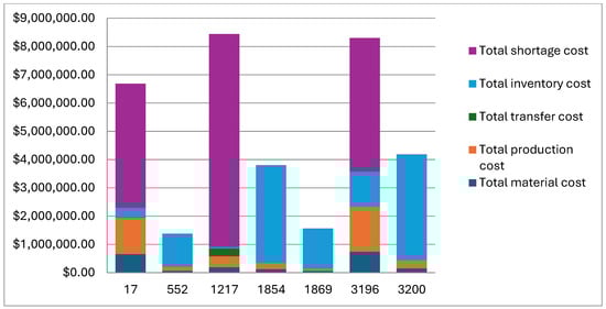
Figure 1.
Supply chain cost components for the selected sample scenarios.
Table 3.
Input parameters for sample scenarios.
5. Multi-Variate Regression Analysis on Simulation Output
Single regression is the estimation of a single regression model between one outcome (dependent) variable and one predictor (independent) variable. If more than one predictor estimates an outcome variable, it is a case of multiple regression. When estimating a regression model for more than one outcome variable and more than one predictor variable, the model is a multi-variate multiple regression [28].
Multi-variate multiple regression (MMR) extends the principles of ordinary multiple regression to simultaneously model multiple dependent variables using a common set of independent predictors. This approach is especially useful when response variables are correlated, as it accounts for interdependencies and controls the Type I error rates across multiple tests [28,29]. In this study, we applied MMR to examine how replenishment policies and demand/lead time variables affect the supply chain costs and inventory levels. The statistical significance of our models was assessed using standard multi-variate tests, such as Wilks’ Lambda, Pillai’s Trace, Lawley-Hotelling Trace, and Roy’s Largest Root, which are widely used in empirical and behavioral research [30]. Similar approaches have been applied in recent supply chain research [24,25]. Summary statistics for both outcome and predictor variables are presented in Table 4 and Table 5.
Table 4.
Summary statistics of the outcome variables (Ys).
Table 5.
Summary statistics of the predictor variables (Xs).
In the following section, four regression models are constructed:
- Supply chain costs as dependent variables, with replenishment parameters as predictors
- Average on-hand stock at each echelon as dependent variables, with replenishment parameters as predictors
- Supply chain costs as dependent variables, with demand and lead time variables as predictors
- Average on-hand stock as a dependent variable, with demand and lead time variables as predictors
5.1. Correlation of Ys
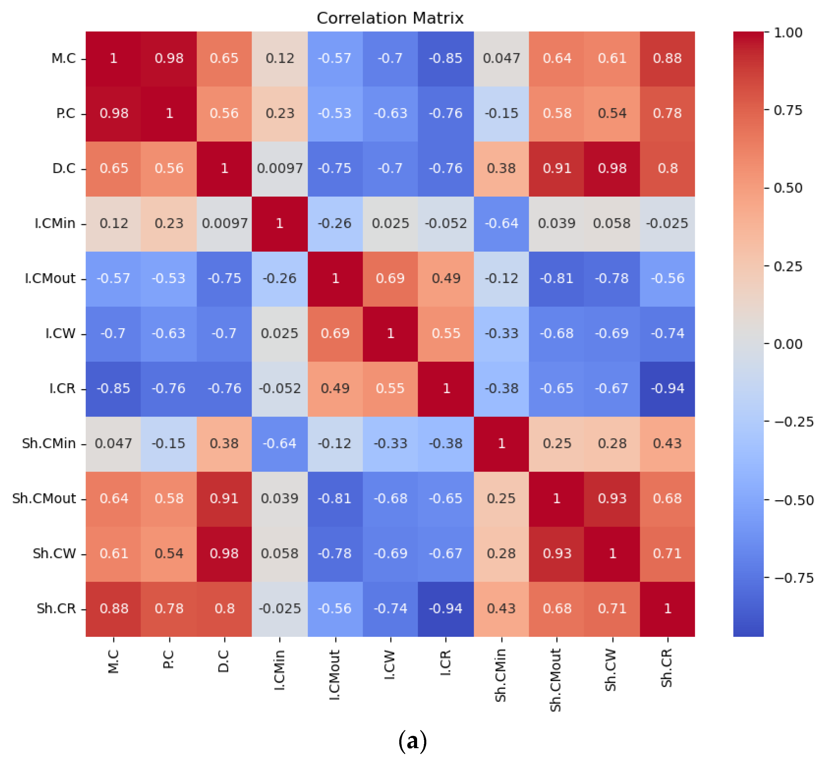
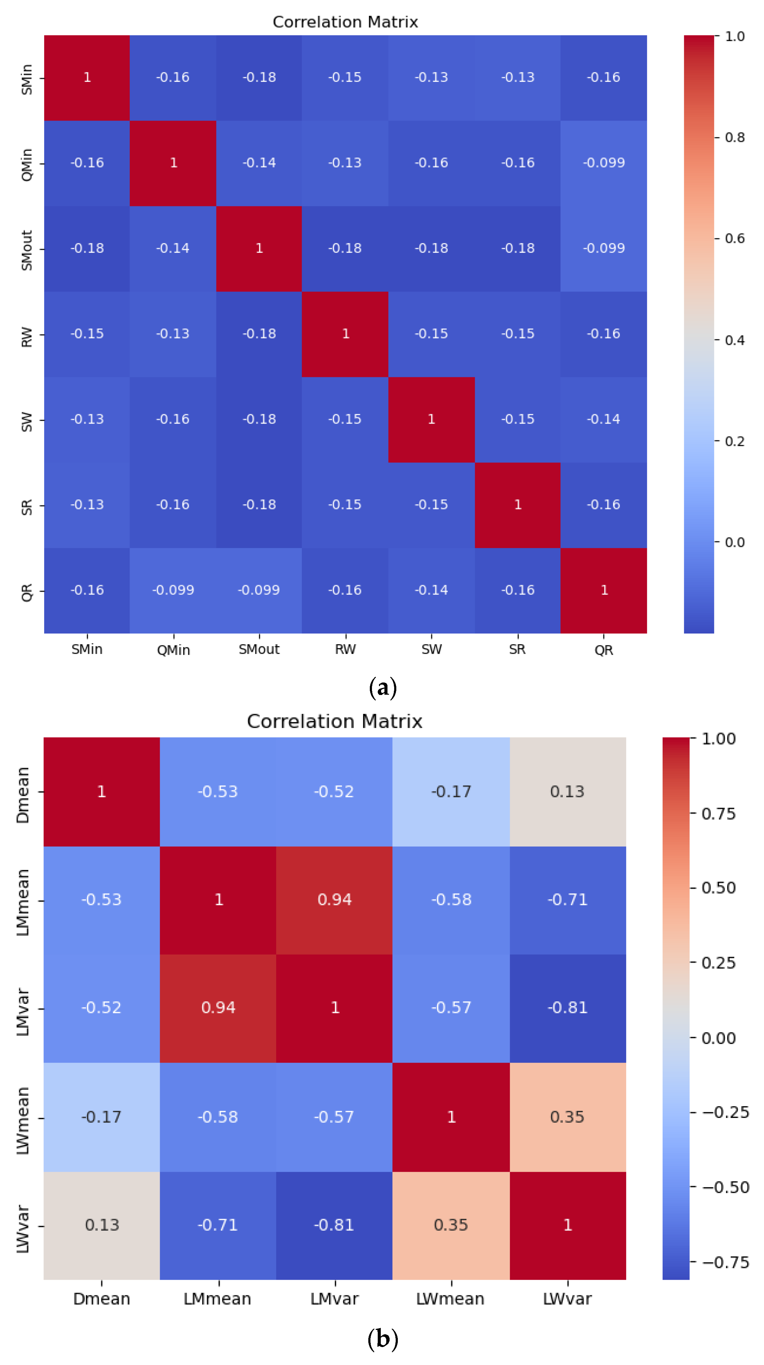
The strong negative correlation between inventory holding costs and shortage costs underscores the classic trade-off between maintaining stock and the risk of stock-outs. Achieving an optimal balance between these costs is essential for effective inventory management. Figure 2 shows the pairwise correlations among the various cost components within the supply chain. Positive correlations are observed among cost components within the same category, such as shortage costs at different echelons—for instance, the correlations between shortage costs at the retailer and manufacturer and between the wholesaler and manufacturer are 0.33 and 0.41, respectively. This suggests that these costs are interrelated and influenced by shared factors. Additionally, the 0.96 positive correlation between material costs and production costs reflects a logical direct relationship. Figure 2 also highlights the relationships between on-hand inventory levels at different echelons: manufacturer input, manufacturer output, wholesaler, and retailer. The correlations are generally weak, with most values close to zero, indicating limited linear relationships. A notable positive correlation of 0.40 exists between retailer and manufacturer output inventories, suggesting a moderate connection between these two stages. Similarly, the correlation of 0.33 between wholesaler and both manufacturer output and retailer inventories suggests some degree of alignment in stock levels. The near-zero and slightly negative correlations for manufacturer input imply little to no direct relationship with the other echelons, indicating independent behavior at this stage. Overall, the results suggest weak-to-moderate interdependencies in inventory levels across the supply chain. This illustrates the behavior of a decentralized supply chain policy, where each echelon operates independently, resulting in less synchronization of inventory levels across the network.
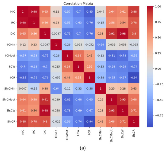

Figure 2.
Correlation of Ys (a) correlation of Sc costs, (b) correlation of on-hand stock at different echelons.
5.2. Correlation of Xs
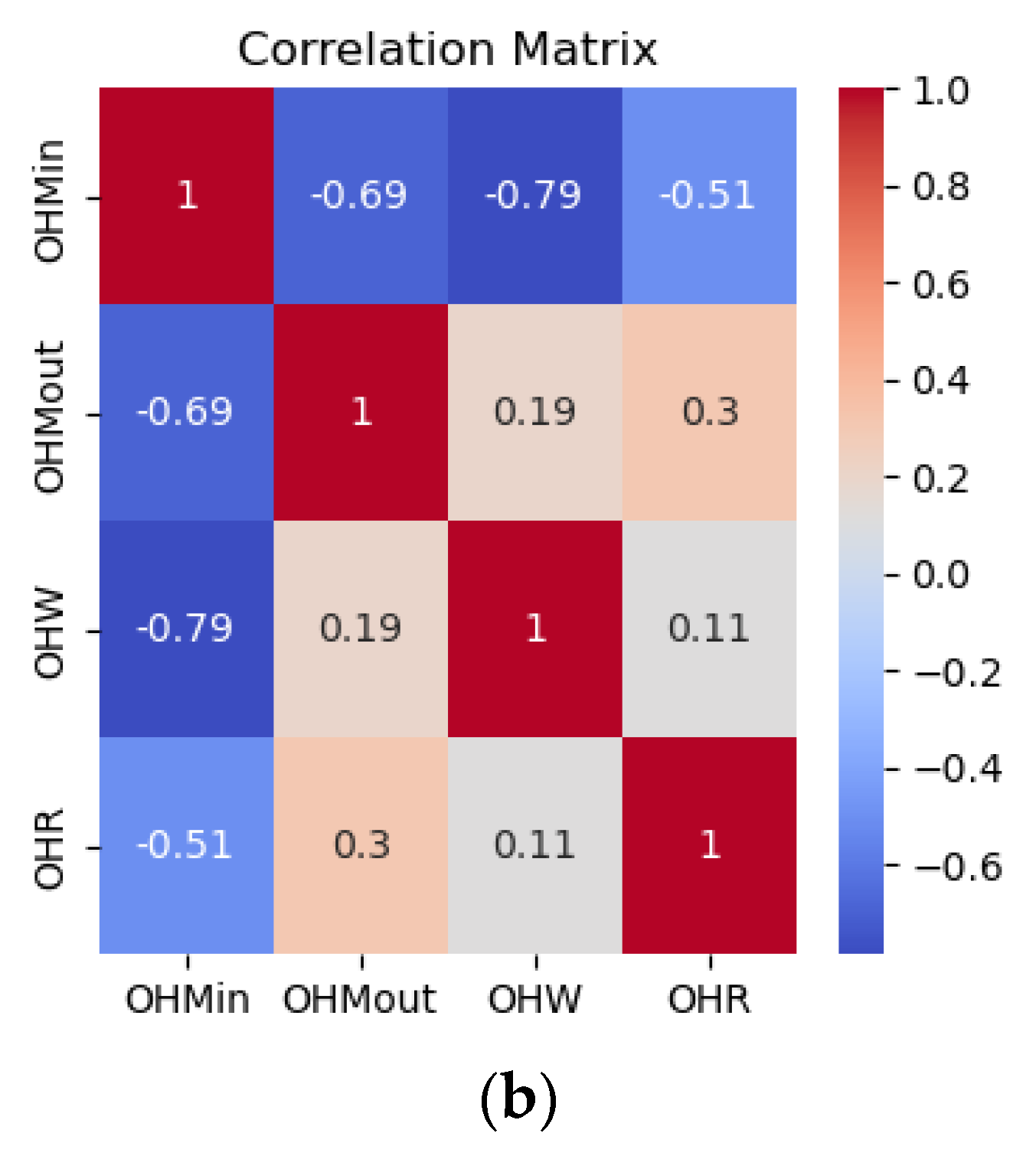
The correlations are generally very low, with most values close to zero, indicating minimal linear relationships between these variables. Little or no correlation between independent variables ensures that each variable contributes unique information to the model. Low multicollinearity improves the stability and interpretability of the regression coefficients and allows for a more accurate estimation of the impact of each independent variable on the dependent variable. Correlations, such as those between order quantities and reorder points across echelons, show almost no relationship, reflecting the decentralized decision-making policy in the supply chain. This decentralized approach likely limits the coordination and alignment of inventory and ordering decisions, resulting in low interdependencies among the variables. Figure 3 shows the relationships between demand, mean lead times, and lead time variances at the manufacturer and wholesaler levels. A strong positive correlation (0.75) between the mean lead time and its variance at the manufacturer indicates that higher average lead times are associated with greater variability, which is attributable to the selected input distributions. This suggests that the inherent variability in lead times is driven by the selected distribution parameters rather than external factors. Conversely, weak or near-zero correlations between the demand and lead time parameters reflect minimal direct linear dependencies. Notably, the mean lead time at the wholesaler exhibits a moderate positive correlation (0.28) with its variance, indicating some variability alignment. The weak correlations between the different echelons suggest limited interdependence across the stages.
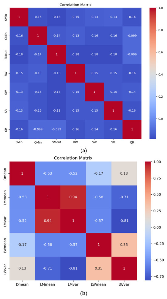
Figure 3.
Correlation of Xs (a) Correlations of replenishment parameters (b) correlation of demand and lead times.
5.3. Regression Model of Supply Chain Costs and Replenishment Parameters
5.3.1. Multi-Variate Analysis of Variance (Tests of Significance)
This section presents the results of a multi-variate regression analysis, where the outcome variables are SC cost items and the input variables are inventory replenishment parameters at different echelons. Table 6 shows the results for various multi-variate test statistics: Wilks’ Lambda (W), Pillai’s trace (P), Lawley-Hotelling trace (L), and Roy’s Largest Root (R). All test statistics (W, P, L, and R) have p-values of 0.00, indicating that the overall model is statistically significant. This implies that the inventory parameters as a group have a significant impact on SC costs.
Table 6.
Test statistics.
5.3.2. The Regression Model of Supply Chain Costs and Replenishment Parameters
The multi-variate regression analysis highlights significant variability in the explanatory power of the models, as indicated by the R2 values, which range from 0.03 to 0.54. The model predicting inventory cost at the manufacturer input stands out with the highest R2 value of 0.54, suggesting that 54% of the variation in the dependent variable is explained by the included predictors (see Table 7). This relatively strong fit implies that the factors included in this model play a crucial role in determining the costs associated with inventory at the manufacturer’s input level. In contrast, models such as material cost, production cost, and shortage cost at the retailer have notably low R2 values (ranging from 0.03 to 0.07), indicating that these models explain only a small fraction of the variance in the outcome variable. This limited explanatory power suggests that additional predictors or alternative model structures are necessary to more effectively capture the underlying complexity of these cost components. The following section presents another multi-variate regression model between SC costs, demand, and lead time variables. The low R2 for the retailer shortage cost is particularly telling. This implies that traditional inventory parameters like reorder level and order quantity alone are insufficient to account for the dynamics affecting shortages at the retail level. This can be attributed to the behavioral and operational factors that are typically unmodeled in parametric regression. For example, retailers may delay reordering despite low inventory levels due to budget cycles, perceived overstock, or supplier negotiation behavior. Additionally, customer-driven factors—like sudden demand surges from promotions or competitor activity—can create stock-outs that are decoupled from internal inventory logic. These complex behaviors can be better captured by agent-based models, behavioral heuristics, or by incorporating soft data (e.g., forecast bias, manual overrides).
Table 7.
The regression model of supply chain costs and replenishment parameters.
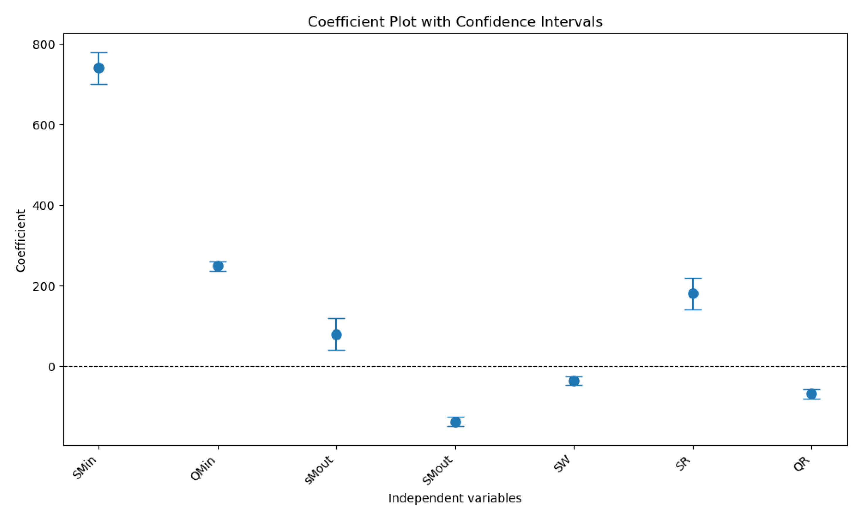
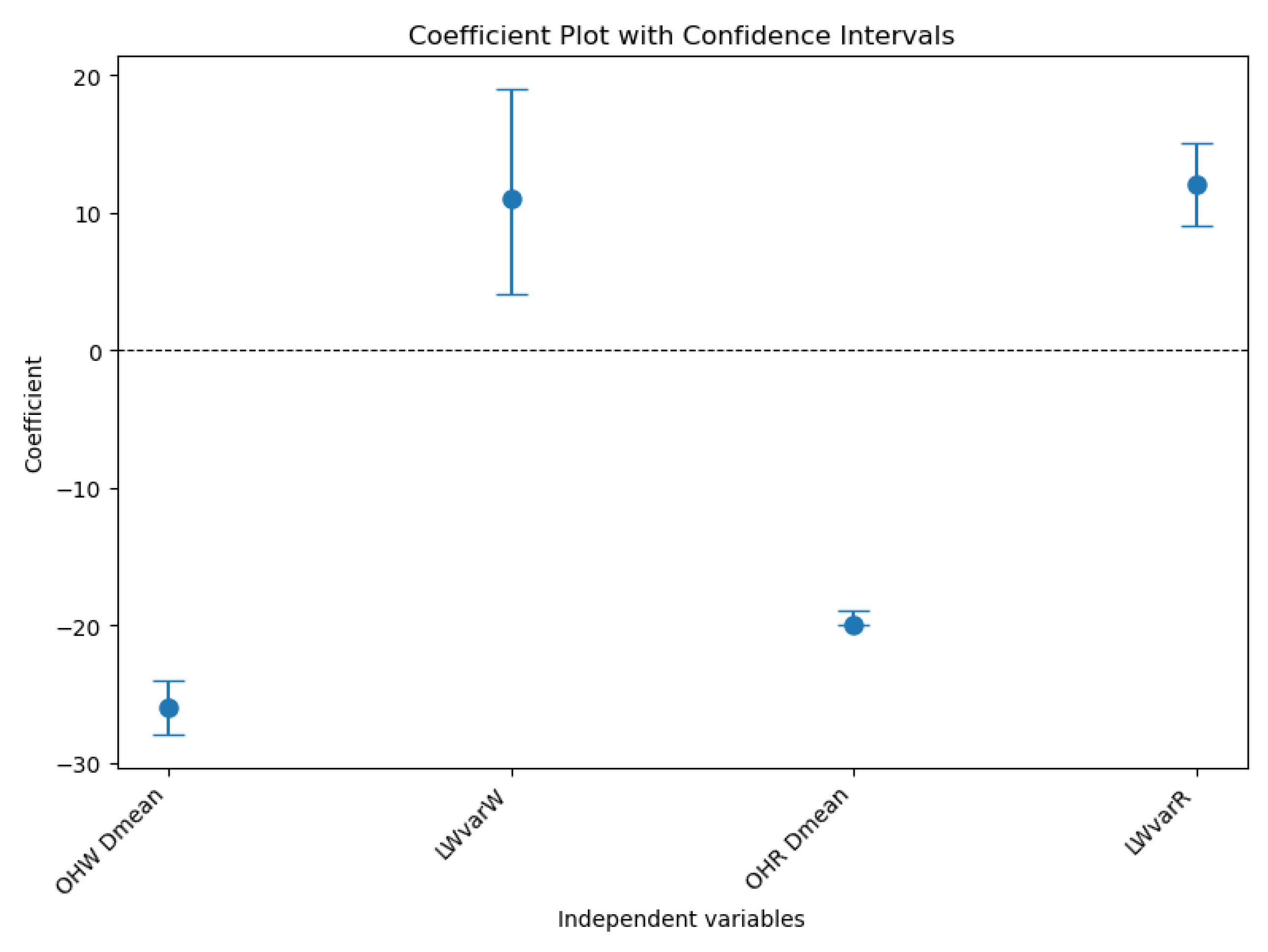
The replenishment parameters at the wholesaler and retailer, specifically SW and QR, emerge as key drivers in multiple models. For instance, SW significantly influences the inventory cost at the manufacturer input with a large positive coefficient and a p-value below 0.01, indicating that increases in wholesaler stock levels are strongly associated with higher inventory costs at the manufacturer. This relationship highlights the importance of inventory positioning and its ripple effect on the supply chain. Similarly, QR (order quantity at the retailer) frequently exhibits a significant negative coefficient, particularly in the inventory cost at the manufacturer input and shortage cost at the retailer models. This negative relationship suggests that larger order quantities at the retailer level are associated with reduced costs, possibly due to economies of scale or reduced ordering frequency, which leads to lower handling or stock-out costs. Additionally, the negative coefficients observed in the models predicting shortage costs at the manufacturer’s input and retailer indicate that certain predictors contribute to cost reductions in these contexts. For example, the negative relationship between the QR and shortage costs suggests that larger order quantities help mitigate stock-outs, thereby lowering the associated costs. Despite these insights, the overall low R2 values in many models underscore the need for further research. A significant portion of the variance remains unexplained, highlighting the potential for incorporating additional variables, such as demand variability, lead times, and external market factors, which may better capture the dynamics of supply chain costs. Figure 4 shows the coefficient plot with confidence intervals for inventory cost at manufacturer output.
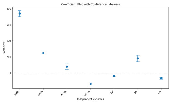
Figure 4.
Coefficient plot with confidence intervals.
5.4. Regression Model of Average On-Hand Stocks and Replenishments Parameters
5.4.1. Multi-Variate Analysis of Variance (Tests of Significance)
This section presents the findings of a multi-variate regression analysis, where the dependent variables represent the average on-hand stock at various supply chain echelons, and the independent variables correspond to inventory replenishment parameters at different echelons. All test statistics yield a p-value of 0.00, confirming that the overall model is statistically significant. This indicates that, collectively, the inventory replenishment parameters exert a significant influence on the average on-hand stock across the different echelons (Table 8).
Table 8.
Test statistics.
5.4.2. The Regression Model of Average On-Hand Stocks and Replenishment Parameters
The R2 values for the models reveal varying explanatory powers across the echelons. Specifically, the average on-hand stock at the manufacturer input achieves the highest R2 value (0.79), indicating that 79% of the variability in the on-hand stock at the manufacturer input is explained by its predictors. The average on-hand at the manufacturer output and wholesaler shows moderate R2 values of 0.43 and 0.45, respectively, while the average on-hand at the retailer has the lowest R2 of 0.32, suggesting a weaker fit and highlighting the potential influence of unaccounted factors at the retailer level. The p-values for all models are 0.00, confirming that the overall regression models are statistically significant Table 9.
Table 9.
The regression model of the average on-hand stock and replenishment parameters.
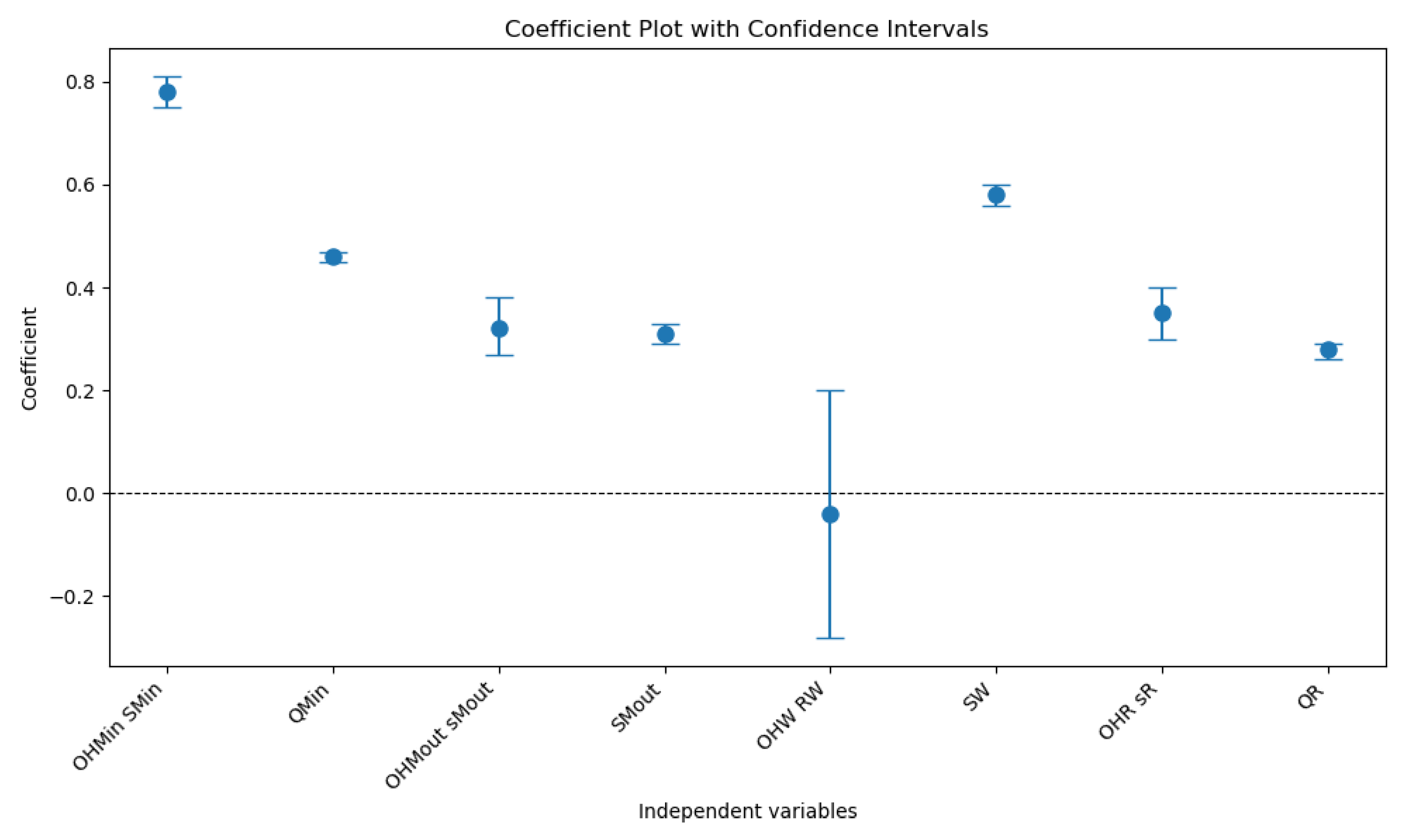
An in-depth examination of the coefficients reveals that different predictors influence the average on-hand stock at each echelon to a varying degree. For the average on-hand at the manufacturer input, the most influential predictors are both replenishment parameters, both with significant p-values, indicating that higher reorder points and order quantities at the manufacturer input level lead to higher on-hand stock. In contrast, other variables, such as replenishment parameters at the manufacturer output, have negligible or insignificant effects. For the average on-hand at the manufacturer output, significant predictors suggest that replenishment policies at the manufacturer output and wholesaler levels contribute positively to stock levels. For the average on-hand inventory at the wholesaler, the primary contributors are the review period and maximum stock level, indicating that reorder levels and stock sizes at the wholesaler are critical factors influencing the on-hand inventory at this echelon. Meanwhile, the average on-hand at the retailer is primarily influenced by the replenishment parameter at this echelon, although the lower R2 value suggests that additional variables not captured in this model may significantly impact retailer-level stocks. Figure 5 shows the coefficient plot with the confidence intervals.
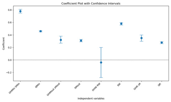
Figure 5.
Coefficient plot with confidence intervals.
The intercept values vary across the models, with manufacturer input having the highest baseline (55.98), followed by wholesaler (43.62), retailer (22.66), and manufacturer output (8.33). These intercepts reflect the inherent baseline levels of on-hand stock that are independent of the predictors. Collectively, the findings highlight the importance of inventory replenishment parameters at each supply chain echelon, particularly at upstream stages, such as the manufacturer input level, where the model exhibits the strongest explanatory power. To improve on-hand stock management, targeted strategies should be implemented based on the identified key predictors. For example, optimizing reorder points and stock capacity at critical echelons can lead to more effective inventory management. Additionally, the relatively lower explanatory power observed at downstream stages, such as the retailer level, suggests the need to explore other factors, such as demand variability, lead time uncertainties, or operational disruptions, to better capture the dynamics influencing on-hand stock levels.
5.5. Regression Model of Supply Chain Costs, Demand, and Lead Time Patterns
5.5.1. Multi-Variate Analysis of Variance (Tests of Significance)
This section reports the results of a multi-variate regression analysis, where the dependent variables represent supply chain SC costs at various echelons, and the independent variables include the demand mean and lead time distribution at different stages of the supply chain. The test statistics consistently yield a p-value of 0.00, indicating that the overall model is statistically significant. This demonstrates that, as a group, the demand mean and lead time distribution have a significant impact on SC costs across the different echelons, as shown in Table 10.
Table 10.
Test statistics.
5.5.2. The Regression Model of Supply Chain Costs, Demand, and Lead Time Patterns
The fit of the models, measured by R2, varies significantly across the echelons. For instance, the shortage cost at the retailer has the highest R2 value (0.92), indicating that 92% of the variance in this cost at this echelon is explained by the independent variables. Moderate explanatory power is observed for the material, production, and total transfer costs, with R2 values of 0.64, 0.49, and 0.35, respectively. However, models for inventory and shortage costs at each echelon show very low R2 values (0.01–0.02), suggesting that these models are ineffective in explaining SC cost variability at these levels (Table 11). These results suggest a nonlinear or interaction-based relationship between input uncertainty (e.g., lead time variance) and operational outcomes, which is not well captured by standard linear regression. Additionally, some supply chain costs may be cushioned or buffered by upstream policies and slack capacity, leading to muted effects of input changes. For example, the manufacturer may overstock or increase batch sizes to buffer against lead-time fluctuations, diluting any one-to-one relationship with holding costs.
Table 11.
The regression model of supply chain costs, demand, and lead time patterns.
Significance testing reveals that most coefficients across echelons are statistically significant, underscoring the relevance of the predictors. Demand mean is consistently significant and exhibits strong coefficients across echelons, indicating that it is a primary driver of SC costs. For example, its coefficients for production cost and shortage cost at the wholesaler are 83,199.42 and 74,711.78, respectively. Lead time variance at the wholesaler is another critical predictor, with significant contributions to costs at key echelons, such as shortage cost at the retailer (coefficient of 82,738.2). However, the impact of the lead time mean is inconsistent; the mean lead time at the manufacturer shows minimal influence on inventory cost. However, it demonstrates moderate significance in terms of transfer costs. Similarly, the mean lead time at wholesaler is significant in some echelons but less impactful overall. These results emphasize the importance of the demand mean and lead time variance as critical factors driving SC costs. The mean demand consistently exerts a significant influence across all echelons, underscoring the need to manage demand variability effectively. Lead time variance, particularly in echelons with higher R2 values, such as shortage costs at the retailer and wholesaler, emerges as another vital factor that can significantly impact cost optimization strategies. In contrast, the inconsistent and often negligible contribution of the lead time mean suggests that this factor may not be as critical for cost management. Figure 6 shows the coefficient plot with the confidence intervals for shortage cost at the wholesaler and the retailer.
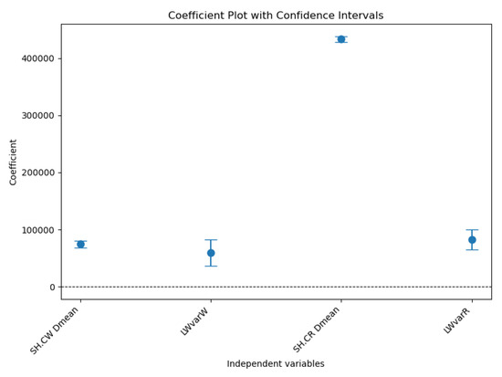
Figure 6.
Coefficient plot with confidence intervals.
5.6. Regression Model of Average On-Hand Stocks and Demand and Lead Time Patterns
Multi-Variate Analysis of Variance (Tests of Significance)
This section presents the results of a multi-variate regression analysis, where the dependent variables represent the average on-hand stocks at various supply chain echelons, and the independent variables include the demand mean and lead time distribution across different stages of the supply chain. The multi-variate regression analysis reveals that the average on-hand stock levels at various supply chain echelons are significantly influenced by certain independent variables. The demand mean and lead time variance at the wholesaler are the most impactful factors, demonstrating statistical significance (Prob > F < 0.05) across all echelons. In contrast, the lead time mean is not statistically significant (Prob > F = 0.54), suggesting minimal influence on stock levels. Lead time variability exhibits borderline significance (Prob > F = 0.12), indicating a potential but inconclusive effect. Different echelons exhibit varying sensitivities, with W and R being more responsive to these factors than P and L. These findings highlight the importance of managing demand variability and lead time variance to optimize inventory levels, while the negligible impact of lead time means warrants further investigation to understand its limited role in supply chain performance (Table 12).
Table 12.
Test statistics.
5.7. The Regression Model of Average On-Hand Stocks and Demand and Lead Time Patterns
The model’s explanatory power, as indicated by R2, varies considerably across echelons. The average on-hand at the retailer demonstrates the highest R2 value (0.43), meaning that 43% of the variability in on-hand stock at this echelon is explained by the predictors. The average on-hand at wholesale follows with a moderate R2 of 0.19, suggesting that the independent variables contribute to explaining stock levels. However, for the average on-hand at the manufacturer, the models exhibit very low explanatory power, indicating that the included variables do not sufficiently account for stock variability at these echelons (Table 13). This contrast may stem from the buffering and batching mechanisms at the upstream stages, which decouple immediate demand or lead time effects from inventory responses. Manufacturers often hold safety stock or use fixed production windows, which makes their inventory levels less sensitive to short-term changes in demand or variability. However, at the retailer and wholesaler levels, lead time variance and demand shifts directly affect inventory positioning. This suggests that downstream echelons are more responsive to external variability, whereas upstream nodes function more as absorbers of system noise. However, even at the retail level, a large portion of stock variability remains unexplained, hinting at the importance of incorporating real-time behavioral or operational signals, such as sales promotions, customer service expectations, or order batching decisions.
Table 13.
The regression model of the average on-hand stocks and demand and lead time patterns.
The demand mean emerges as a key predictor of the average on-hand stock at wholesaler and retailer. It is statistically significant as P > ∣t∣ = 0.00 at these echelons and is negatively associated with on-hand stock, with coefficients of −26.01 and −19.54, respectively. This indicates that a higher demand mean reduces inventory levels, reflecting improved efficiency or optimized stock replenishment strategies. However, for the average on-hand at the manufacturer (P > ∣t∣ = 0.09 and P > ∣t∣ = 0.26), the demand mean is less significant, highlighting its limited influence on stock levels in upstream echelons.
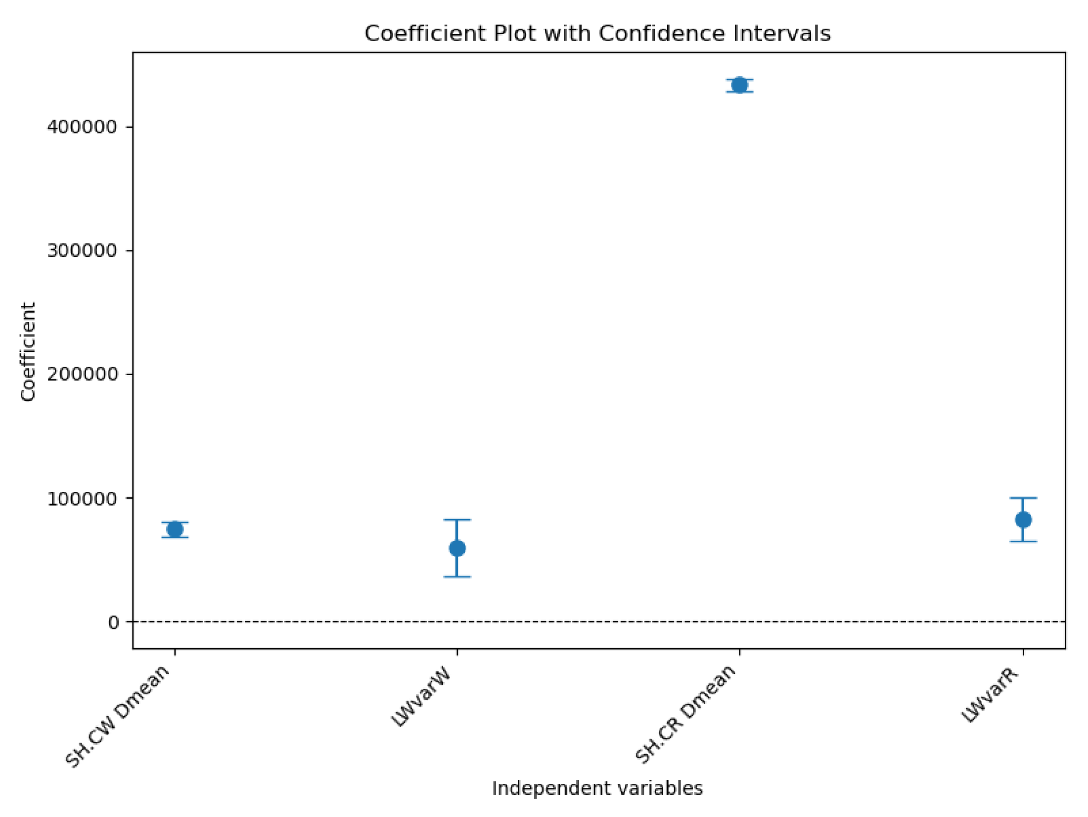
The lead time variance at the wholesaler also plays a significant role, particularly for the average on-hand at the wholesaler and retailer, where it has positive and significant effects (P > ∣t∣ = 0.00). At the retailer, the coefficient of 11.96 suggests that higher variability in lead time increases inventory levels to buffer against uncertainty. Conversely, the lead time mean and variance at the manufacturer have minimal or non-significant effects across all echelons, implying that these factors do not meaningfully contribute to on-hand stock variability in this context. Figure 7 shows the coefficient plot with confidence intervals for on-hand stock at the wholesaler and the retailer.

Figure 7.
Coefficient plot with confidence intervals.
6. Conclusion Recommendations for Future Research
This study advances the understanding of inventory dynamics in decentralized multi-echelon supply chains by integrating discrete-event simulation with multi-variate regression analysis. By simulating a three-echelon supply chain and analyzing various inventory policy scenarios, this study identifies how changes in inventory parameters at each echelon affect overall supply chain performance, specifically in terms of inventory costs and on-hand stock levels. The analysis demonstrates that inventory policy settings have an echelon-specific impact. While replenishment parameters explain a significant portion of cost and stock variability at upstream nodes (e.g., manufacturer input), their explanatory power diminishes at downstream levels, where demand variability and behavioral factors play a more dominant role. These findings highlight the limitations of deterministic control policies in decentralized systems and indicate the need for more adaptive and responsive strategies in real-world settings.
6.1. Contribution to Existing Knowledge
This research contributes a simulation-based analytical framework for evaluating inventory performance in decentralized MESCs. By combining discrete-event simulation with multi-variate regression, this study provides a statistically grounded method for identifying key inventory drivers influencing supply chain costs and stock levels. This study addresses a gap in the literature regarding the interplay between decentralized decision-making and echelon-specific inventory outcomes.
6.2. Managerial Implications
These findings provide practical insights for supply chain managers. This study investigates the impact of inventory policy parameters, specifically reorder levels, order quantities, and review intervals, on the overall performance of a multi-echelon supply chain. This study used a simulation of a three-echelon supply chain under varying demand patterns and inventory policies, combined with multi-variate regression analysis. The results offer practical recommendations for supply chain managers:
- Retailer-level decisions (e.g., increasing reorder quantities) significantly reduce stock-outs and upstream costs.
- Wholesaler review intervals influence not only local stock levels but also upstream inventory buildup.
- Buffering strategies should be tailored based on demand and lead time variability, particularly at the W and R levels.
Furthermore, this study underscores the importance of coordination and information sharing across echelons to mitigate inefficiencies such as overstocking or shortages. This study supports the use of data-driven inventory planning to balance cost efficiency and service-level performance in decentralized supply chains.
6.3. Future Research Directions
Although this study adopts a single-product, three-echelon supply chain structure to ensure analytical clarity and computational feasibility, this scope limits its generalizability to more complex systems. However, the simulation-regression approach is scalable and can be extended to multiproduct, multi-segment, or networked supply chains to better reflect real-world complexity and explore advanced dynamics, such as resource pooling and echelon interdependencies.
Future work should utilize primary data from diverse industries to validate and calibrate the simulation model more accurately. Although our parameterization is based on existing empirical studies, it remains largely sector-specific.
From an analytical standpoint, integrating machine learning approaches such as reinforcement learning could enable real-time adaptive inventory policies. Stochastic optimization can enhance decision-making under uncertainty. Barriers to implementation—such as data quality, integration costs, and organizational readiness—should also be addressed. In decentralized structures, collaboration tools and digital infrastructure (e.g., ERP and cloud platforms) are essential for scaling these models.
Sustainability is another critical area. Incorporating environmental costs and circular economy practices (e.g., remanufacturing) would support more eco-efficient supply chains. Technologies like IoT and blockchain offer opportunities to enhance visibility and enable decentralized coordination through smart contracts and real-time tracking.
Lastly, behavioral aspects, such as decision-making biases, negotiation strategies, and trust dynamics, could add depth to future models. Exploring intermittent, promotion-driven, or service-sensitive demand patterns would also broaden the model’s practical applicability. These directions will enrich both the theoretical understanding and practical implementation of inventory management in decentralized, resilient, and sustainable supply chains.
Funding
This research was funded by Princess Nourah bint Abdulrahman University Researchers Supporting Project number (PNURSP2025R914).
Data Availability Statement
The original contributions presented in this study are included in the article. Further inquiries can be directed to the author.
Acknowledgments
The author extends her appreciation to the support of funding received from Princess Nourah bint Abdulrahman University Researchers Supporting Project number (PNURSP2025R914), Princess Nourah bint Abdulrahman University, Riyadh, Saudi Arabia.
Conflicts of Interest
The author declares no conflict of interest.
References
- He, S.H. Coordination of Production Planning in Multiechelon Supply Chains: A Simulation Approach. Int. J. Simul. Model. 2024, 23, 728–739. [Google Scholar] [CrossRef]
- Nielsen, P.; Michna, Z.; Saha, S. A note on the stochastic nature of lead times in multi-echelon supply chains. Int. J. Logist. Syst. Manag. 2020, 36, 399–413. [Google Scholar] [CrossRef]
- Cuong, T.N.; Kim, H.S.; Bao Long, L.N.; You, S.S. Decision support system for managing multi-echelon supply chain networks against disruptions using adaptive fractional order control algorithm. RAIRO—Oper. Res. 2023, 57, 787–815. [Google Scholar] [CrossRef]
- César, J.; Geraldo, A.; Mateus, R.; Alves, J.C.; Mateus, G.R. Multi-echelon Supply Chains with Uncertain Seasonal Demands and Lead Times Using Deep Reinforcement Learning. arXiv 2022, arXiv:2201.04651. [Google Scholar] [CrossRef]
- Paine, J. Behaviorally Grounded Model-Based and Model Free Cost Reduction in a Simulated Multi-Echelon Supply Chain. arXiv 2022, arXiv:2202.12786. [Google Scholar] [CrossRef]
- Mohammed, I.; Mandal, J. The Impact of Lead Time Variability on Supply Chain Management. Int. J. Supply Chain Manag. 2024, 8, 41–55. [Google Scholar] [CrossRef]
- Debnath, A.; Sarkar, B. Supply Chain Model Having Stochastic Lead Time Demand with Variable Production Rate and Demand Dependent on Price and Advertisement. RAIRO—Oper. Res. 2024, 58, 2645–2667. [Google Scholar] [CrossRef]
- Alaswad, S.; Salman, S.; Alhashmi, A.; Almarzooqi, H.; Alhammadi, M. The Effect of Demand Variability on Supply Chain Performance. In Proceedings of the International Conference on Modeling, Simulation and Applied Optimization, Manama, Bahrain, 15–17 April 2019. [Google Scholar] [CrossRef]
- Caballero Morales, S.O.; Carreón-Nava, L.-F. Multi-retailer Sales Model under Uncertain Demand in a Pharmaceutical Two-Echelon Supply Chain with Vendor Managed Inventory System. Int. J. Comb. Optim. Probl. Inform. 2022, 13, 114–128. [Google Scholar] [CrossRef]
- Lejarza, F.; Kelley, M.T.; Baldea, M. Feedback-Based Deterministic Optimization Is a Robust Approach for Supply Chain Management under Demand Uncertainty. Ind. Eng. Chem. Res. 2022, 61, 12153–12168. [Google Scholar] [CrossRef]
- Sazvar, Z.; Zokaee, M.; Tavakkoli-Moghaddam, R.; Salari, S.A.-S.; Nayeri, S. Designing a sustainable closed-loop pharmaceutical supply chain in a competitive market considering demand uncertainty, manufacturer’s brand and waste management. Ann. Oper. Res. 2022, 315, 2057–2088. [Google Scholar] [CrossRef] [PubMed]
- Lindahl, S.B.; Babi, D.K.; Gernaey, K.V.; Sin, G. Integrated capacity and production planning in the pharmaceutical supply chain: Framework and models. Comput. Chem. Eng. 2023, 171, 108163. [Google Scholar] [CrossRef]
- Yani, L.P.E.; Aamer, A. Demand forecasting accuracy in the pharmaceutical supply chain: A machine learning approach. Int. J. Pharm. Healthc. Mark. 2022, 17, 1–23. [Google Scholar] [CrossRef]
- Alidoost, F.; Mustafee, N.; Monks, T.; Harper, A. Simulation in healthcare supply chains with perishable products: A scoping review. J. Oper. Res. Soc. 2025, 1–36. [Google Scholar] [CrossRef]
- Avci, Ö. A Study to Examine the Importance of Forecast Accuracy to Supply Chain Performance: A Case Study at a Company from the FMCG Industry. Bachelor’s Thesis, University of Twente, Enschede, The Netherlands, 2019. [Google Scholar]
- Bouazza, S.; Amari, S.; Addouche, S. Linear Min-Plus system control under generalized mutual exclusion constraints: Application to managing the replenishment policy of a supply chain in the presence of disturbances. In Proceedings of the International Conference on Control, Decision and Information Technologies, Valletta, Malta, 1–4 July 2024; pp. 1335–1340. [Google Scholar] [CrossRef]
- Wang, L.; Chen, H. Optimization of a Periodic Review Joint Replenishment Policy for a Stochastic Inventory System. In Advances in Production Management Systems 2021; Springer: Cham, Switzerland, 2021; Volume 630, pp. 493–501. [Google Scholar] [CrossRef]
- Lawrence, A.S.; Melikov, A.; Sivakumar, B. Analysis and optimization of hybrid replenishment policy in a double-sources queueing-inventory system with MAP arrivals. Ann. Oper. Res. 2023, 331, 1249–1267. [Google Scholar] [CrossRef]
- Farhangi, H. Multi-Echelon Supply Chains with Lead Times and Uncertain Demands: A Lot-Sizing Formulation and Solutions. Oper. Res. Forum 2021, 2, 46. [Google Scholar] [CrossRef]
- Kost, A.R.; Vergara, H.A.; Porter, J.D. A quantitative analysis of simultaneous supply and demand disruptions on a multi-echelon supply chain. Int. J. Ind. Syst. Eng. 2024, 46, 556–583. [Google Scholar] [CrossRef]
- Vostriakova, V.; Kononova, O.; Kravchenko, S.; Ruzhytskyi, A.; Sereda, N. Optimization of Agri-Food Supply Chain in a Sustainable Way Using Simulation Modeling. Int. J. Comput. Sci. Netw. Secur. 2021, 21, 245–256. [Google Scholar]
- Kim, S.; Choi, Y.; Kim, S. Simulation Modeling in Supply Chain Management Research of Ethanol: A Review. Energies 2023, 16, 7429. [Google Scholar] [CrossRef]
- Zheng, Y.; Liu, L.; Shi, V.; Huang, W.; Liao, J. A Resilience Analysis of a Medical Mask Supply Chain during the COVID-19 Pandemic: A Simulation Modeling Approach. Int. J. Environ. Res. Public Health 2022, 19, 8045. [Google Scholar] [CrossRef]
- Liu, M. The research of the impact on consumer perceived value of postponement strategy—Based on multiple linear regression analysis. In Proceedings of the 5th International Conference on E-Commerce and Internet Technology, ECIT 2024, Changsha, China, 15–17 March 2024. [Google Scholar] [CrossRef]
- Qiu, Z.; Zhang, M.; Zhang, R. The Impact of COVID-19 on Logistics in Context of Regression Analysis. BCP Bus. Manag. 2023, 38, 1138–1144. [Google Scholar] [CrossRef]
- Wang, Y. Linkages Between Metropolitan Economy and Modem Logistics Based on Linear Regression Analysis. In Proceedings of the 2020 2nd International Conference on Economic Management and Model Engineering (ICEMME), Chongqing, China, 20–22 November 2020; pp. 64–67. [Google Scholar] [CrossRef]
- Silver, E.A.; Pyke, D.F.; Peterson, R. Inventory Management and Production Planning and Scheduling, 3rd ed.; John Wiley: New York, NY, USA, 1998; Available online: https://scirp.org/reference/referencespapers?referenceid=1568920 (accessed on 11 June 2025).
- Rencher, A.C.; William, F.C. Methods of Multivariate Analysis, 3rd ed.; John Wiley & Sons: Hoboken, NJ, USA, 2012; pp. 1–758. [Google Scholar] [CrossRef]
- Tabachnick, B.G.; Fidell, L.S. Using Multivariate Statistics, 7th ed.; Pearson Education: London, UK, 2019; Available online: https://www.scirp.org/reference/referencespapers?referenceid=3557877 (accessed on 11 June 2025).
- Hair, J.F.; Babin, B.J.; Anderson, R.E.; Black, W.C. Multivariate Data Analysis, 8th ed.; England Pearson Prentice: London, UK, 2019; Available online: https://www.scirp.org/reference/referencespapers?referenceid=2975006 (accessed on 11 June 2025).

Disclaimer/Publisher’s Note: The statements, opinions and data contained in all publications are solely those of the individual author(s) and contributor(s) and not of MDPI and/or the editor(s). MDPI and/or the editor(s) disclaim responsibility for any injury to people or property resulting from any ideas, methods, instructions or products referred to in the content. |
© 2025 by the author. Licensee MDPI, Basel, Switzerland. This article is an open access article distributed under the terms and conditions of the Creative Commons Attribution (CC BY) license (https://creativecommons.org/licenses/by/4.0/).