Abstract
To realize accurate ladle pouring, an analytical model of the constant flow rate pouring was established. By integrating a user-defined function (UDF), a CFD simulation model of the constant flow rate pouring was established to investigate the liquid steel pouring behavior under different inner wall inclination angle α, initial liquid volume Vc, and target flow rate q. Finally, the accuracy of the analytical model and the simulation model was verified through experiments. The results show that the experimental results agree well with the theoretical and simulation results, which verify the accuracy of the analytical model and the simulation model. Moreover, the simulation results indicate that increasing both α and Vc leads to an increase in the pouring flow rate. To achieve a stable pouring process and a constant flow rate value, a proper α, Vc and qt should be selected. In this study α = 7.5° Vc = 70% Vcapacity and q in the range of 0.10–0.12 m3/s are proper. To realize constant flow rate pouring, a time-variant ladle angular velocity is obtained and it can be adjusted by the motor speed. Therefore, different constant flow rates could be acquired by adjusting the motor speed, which provide guidance to the casting technology.
1. Introduction
An accurate pouring process plays a crucial role in the casting technology. Conversely, improper pouring, such as the fluctuation in flow rate or the presence of residual liquid steel, could result in defects like inclusions and porosity, which, in turn, results in an increased scrap rate and an increased production cost. However, traditional pouring methods rely heavily on the experience and skill of operators, which would result in a high defect rate. Consequently, to ensure high-quality casting production and reduce the influence of human factors, the constant flow rate pouring technology has become a key focus in casting research [1,2,3]. This technology encompasses various control methods, including quality control, electrode control, volume control, time control, demonstration-based reproduction control, and image processing control [4,5,6,7,8].
Wei et al. [9] investigated the liquid steel pouring process using a computational fluid dynamics (CFD) simulation model. The results showed that the two-phase flow model could effectively simulate the liquid steel pouring process, which confirmed the feasibility of CFD simulation. Han et al. [10] further utilized a CFD simulation model to analyze the dynamic changes in the flow field, temperature field, and phase interfaces during ladle pouring at a constant rotational speed in two-dimensional space. Jin et al. [11] found that operating the tilting pouring machine at a fixed angular velocity could not realize a constant flow rate pouring. However, continuously adjusting the angular velocity of the ladle could achieve it.
Nobutoshi [12] implemented a flow rate control system based on differential flatness in an automatic pouring machine and experimentally validated its effectiveness in mitigating disturbances. Cheng [13] experimentally investigated a pneumatic constant flow rate pouring system. The results showed that the pouring flow rate increases with the air flow rate, and it can be controlled by adjusting the pouring duration. Gao [14] introduced a machine vision-based image processing technology for automatic pouring and proposed an edge extraction method for metal level detection in pouring images.
However, stable and accurate pouring has not yet been realized by controlling the ladle angular velocity. Thus, to realize accurate ladle pouring, an analytical model of the constant flow rate pouring was established, and a control curve of the ladle angular velocity was acquired. By integrating a user-defined function (UDF), a CFD simulation model of the constant flow rate pouring was established to investigate the liquid steel pouring behavior under different inner wall inclination angles, initial liquid volumes, and target flow rates. Finally, the accuracy of the analytical model and the simulation model was verified through experiments.
2. Analytical Model of Pouring Process of the Steel Ladle
After the steel ladle is designed, the structural parameters remain constant except for the initial liquid volume, as shown in Figure 1.
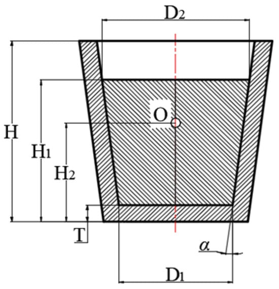
Figure 1.
Schematic diagram of the ladle structure.
The ladle pouring process can be divided into three stages. During these three stages, the residual liquid volume in the ladle changes over time. In the first stage, the residual liquid volume remains unchanged, and no liquid flows out of the ladle, as shown in Figure 2a. In the second stage, the liquid begins to flow out of the ladle and the residual liquid volume decreases, and the ladle bottom is still fully submerged in liquid steel, as shown in Figure 2b. In the third stage, the ladle bottom is exposed. Meanwhile, the liquid keeps flowing out of the ladle, and the residual liquid volume continues decreasing, as shown in Figure 2c.
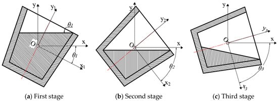
Figure 2.
Plot of change in residual liquid volume.
During the pouring process, the flow characteristics and the liquid distribution vary at each stage. Typically, the liquid steel flows in the shape of an obliquely truncated cone or an irregular horseshoe as it exits the ladle. Due to the absence of an accurate volume calculation formula, liquid steel is often modeled as a cylinder [15]. The diameter D of the cylinder is calculated as D = (D1 + D2)/2, where D1 and D2 represent the diameters at the top and bottom of the ladle, respectively. In ladle design, this assumption is reasonable due to the generally small taper. Additionally, the initial liquid volume is typically assumed to be 70% of the total ladle capacity. Using the relationship between the ladle rotation angle θ and the residual liquid volume, the residual liquid volume at any given θ can be calculated after establishing an analytical model.
2.1. Analytical Model of the Residual Liquid Volume During the Pouring Process
In the first stage (0° < θ < θ1), the ladle starts to rotate, but no liquid steel flows out, as the surface of the liquid steel has a certain distance from the outlet. θ1 is the critical angle of the first stage. When the ladle rotates to θ1, the liquid steel begins to flow out of the ladle. The residual liquid volume in the first stage is set to V0, as shown in Figure 2a.
The critical value of the ladle rotation angle θ1 is:
At this time, the residual liquid volume V0 in the ladle is:
In the second stage (θ1 ≤ θ < θ2), the liquid steel in the ladle is in the shape of an obliquely truncated cone, set the residual liquid volume in the second stage to V1, as shown in Figure 2b.
The critical value of the ladle rotation angle θ2 is:
At this time, the residual liquid volume V1 in the ladle is:
In the third stage (θ2 ≤ θ < 90°), the liquid steel continues flowing out of the ladle, and the steel in the ladle is in the shape of an irregular horseshoe until the pouring completion, as shown in Figure 2c.
To simplify the calculation, the shape is modeled as a regular cylinder obliquely truncated by the residual diagonal tangent. The coordinate axes are established, as shown in Figure 3. The residual volume of the ladle is determined through calculus.
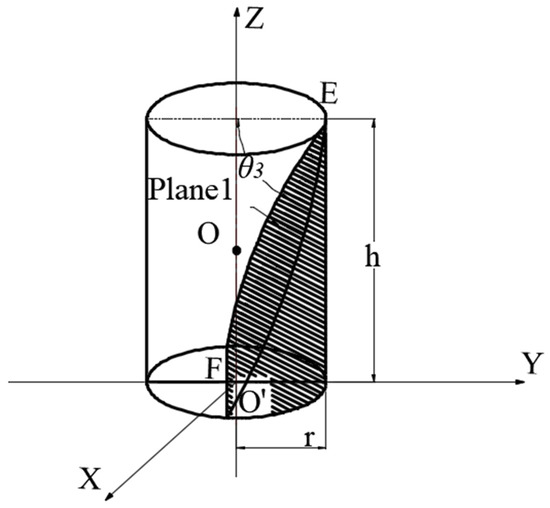
Figure 3.
Simplified ladle coordinate system.
There is a liquid surface plane 1, which passes through points E(0, r, h) and point F(0, r − htanθ, h). Set the equation of plane 1 to Ax + By + Cz = D. This equation of plane 1 can be solved by finding the normal vector of plane 1 as follows:
where r = D/2, a = D/2 − h/tanθ.
The residual liquid volume V2 in the ladle is as follows:
Summarizing the above three stages, the analytical model of the residual liquid volume V in the ladle at any ladle rotation angle θ can be obtained.
2.2. Analytical Model of the Flow Rate During the Pouring Process
By taking the first-order derivative of the residual liquid volume with respect to time and then taking the absolute value of this derivative, the flow rate q is obtained. Similarly, the flow rate changes over time during the pouring process, and the flow rates at the three stages q0, q1, and q2 are also different.
In the first stage (0° < θ < θ1), V0 = Vc. The flow rate q0 can be calculated as
In the second stage (θ1 ≤ θ < θ2), the flow rate q1 can be calculated as follows:
In the third stage (θ2 ≤ θ < 90°), the flow rate q2 can be calculated as follows:
where .
Summarizing the above three stages, the analytical model of the flow rate q at any ladle rotation angle θ as well as the ladle angular velocity ω can be obtained.
To realize constant flow rate pouring, a time-invariant ladle angular velocity ω is required. Therefore, the ladle angular velocity ω becomes a function of the ladle rotation angle θ, in which ω can be calculated according to any ladle rotation angle θ.
3. Simulation Model of Pouring Process of the Steel Ladle
3.1. CFD Simulation Setting
The simulation was conducted using ANSYS Fluent 2022 R1 on a workstation equipped with dual Intel Xeon Gold 6248R CPUs (48 cores) and 256 GB of RAM. A User-Defined Function (UDF) for the ladle rotation speed was written using the compiler within Fluent. The convergence criterion is set as the residual being less than 10−4.
To study the flow behavior during the pouring process, a geometrical model of the ladle was constructed (in it, D1 = 2305 mm, D2 = 2985 mm, H = 3740 mm, H1 = 2927 mm, T = 350 mm, and the inner wall inclination angle α = 7.5°), as shown in Figure 4. The model consists of the following three domains: the liquid domain inside the ladle, the air domain inside the ladle, and the air domain outside the ladle, as shown in Figure 5. During the meshing process, a tetrahedral mesh is generated using the patch-conformal algorithm. For the ladle domain, the mesh size is 70 mm, while for the air domain, it is 200 mm. The total number of nodes is 173,699, and the total number of cells is 956,763. Meanwhile, the initial liquid volume Vc is set to 14,226 L, and the total pouring time t is set to 110 s. The liquid steel does not flow out of the ladle in the range of 0–20 s, and it begins to flow out at t = 20 s and completely flows out at t = 110 s.
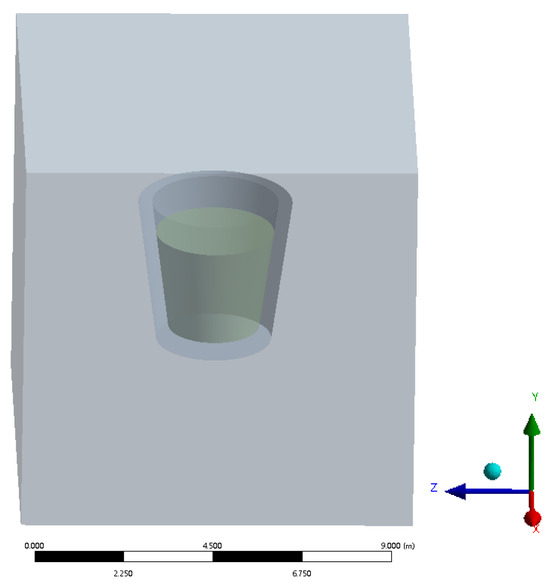
Figure 4.
Ladle model.
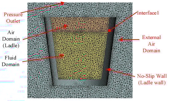
Figure 5.
Divided meshes.
To verify mesh independence and eliminate the influence of mesh number on calculation accuracy, four sets of meshes were generated. The number of meshes in each set was 420,235, 550,378, 956,763, and 1,131,109, corresponding to Mesh No. 1, No. 2, No. 3, and No. 4, respectively. Error analysis was then carried out on the pouring flow rates calculated using these four sets of meshes, and the results are shown in Table 1.

Table 1.
Mesh independence test results.
The results show that the calculation error of the s flow rate between Mesh No. 1 and No. 2 is 0.79%; between Mesh No. 2 and No. 3 is 0.95%; and between Mesh No. 3 and No. 4 is 0.025%. Through comparing the calculation errors, it is evident that the calculation error between Mesh No. 3 and No. 4 is extremely small, indicating that the impact of mesh number on the solution results can be ignored. Given the limitations of computing capacity, Mesh No. 3 which has a mesh number of 956,763 was selected for subsequent simulation calculations.
The viscosity and the density of the liquid steel are set to 0.0062 Pa/s and 7138 kg/m3, respectively [10]. As an isothermal model was adopted, thermal properties were not relevant to the flow simulation. The initial temperature of 1600 K was only used for phase initialization (liquid steel). The air is treated as an incompressible gas, and its viscosity, thermal conductivity, specific heat capacity, and molar mass are set to 1.7894 × 10⁻⁵ Pa/s, 0.0242 W/m K, 1006.4 J/kg K and 28.9 g/mol, respectively. The boundary conditions are defined as follows: (1) the upper surface boundary of the air domain is specified as a pressure outlet, with its value set to the atmospheric pressure; (2) the boundary between the liquid domain inside the ladle and the air domain is defined as an internal boundary. Additionally, the ladle outlet surface in contact with the air is also defined as an internal boundary; (3) all the other boundaries are defined as static, no-slip, adiabatic wall surfaces. The realizable k-ε model and volume of fluid (VOF) model are used to track the phase interface between the liquid steel and the air.
The liquid domain inside the ladle is initialized at 1600 K (the temperature of the liquid steel), while all the other domains are set to 300 K. The external pressure is set to the standard atmospheric pressure of 101,325 Pa. Gravity is applied in the negative direction along the Y-axis, with the value of 9.8 m/s2. The pressure-velocity coupling is handled using the SIMPLE algorithm. For investigating the flow behavior, a dynamic mesh technology was used. The number of time steps is 250 s, the time step size is 0.08 s, the maximum number of iterations is 5, and the turbulence model is adopted. A diffusion smoothing method is applied, and the meshes are periodically re-meshed to maintain high quality. The geometrical parameters are substituted into Equation (7) to establish a relationship between the ladle rotation angle θ and time, as shown in Figure 6. Simultaneously, the relationship between the ladle angular velocity ω and time is obtained, as shown in Figure 7.
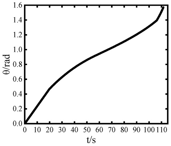
Figure 6.
Change curve of the ladle rotation angle θ with time.
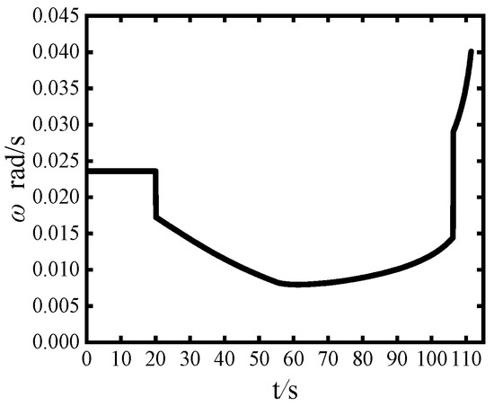
Figure 7.
Change curve of the ladle angular velocity ω with time.
In the range of 0–20 s, the ladle angular velocity remains constant, and the liquid steel has not yet begun to flow out of the ladle. In the range of 20–110 s, the angular velocity first decreases, then gradually increases, and finally sharply increases. To accurately define the ladle angular velocity over time, a user-defined function (UDF) was used. By defining the boundary as a rotating body around a fixed axis, the dynamic behavior during the pouring process can be precisely captured.
3.2. Transient Flow Field During the Constant Flow Rate Pouring Process
During the constant flow rate pouring process, the change in the phase interface is a crucial factor affecting the flow characteristics. The simulation results indicate that the whole pouring process can be divided into four stages. Each stage reflects different physical phenomena and flow characteristics of the liquid steel. Next, the phases are analyzed in detail at the following four stages, as shown in Figure 8.
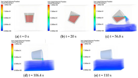
Figure 8.
Transient phase interface during constant flow rate pouring process.
- (1)
- The first stage of the pouring process (0~20 s). The ladle begins to rotate, and the angular velocity remains constant. The liquid steel starts to flow slowly on the upper surface, with the flow mainly concentrated in a small area inside the ladle.
- (2)
- The second stage of the pouring process (20~56.8 s). The liquid steel begins to flow out of the ladle, with the flow concentrated around the ladle outlet.
- (3)
- The third stage of the pouring process (56.8~106.4 s). As the ladle rotation angle increases, the residual liquid volume decreases and the bottom of the ladle becomes exposed, so the ladle angular velocity gradually increases.
- (4)
- The fourth stage of the pouring process (106.4~110 s). The residual liquid volume further decreases until the pouring is complete, and little liquid steel is left in the ladle.
In addition, a cross-section of the ladle is presented to observe the velocity change in the liquid steel during the constant flow rate pouring process, as shown in Figure 9.
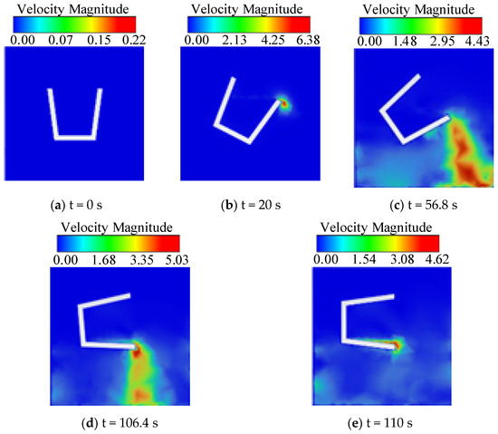
Figure 9.
Transient liquid velocity during constant flow rate pouring process.
- (1)
- The first stage of the pouring process (0~20 s). Initially, the liquid velocity was zero. When the ladle begins to rotate, liquid velocity occurs inside the ladle, while no liquid velocity happens outside the ladle.
- (2)
- The second stage of the pouring process (20~56.8 s). The liquid steel begins to flow out of the ladle, so liquid velocity occurs outside the ladle. The liquid velocity gradually increases with the increase in the falling height due to gravity. Meanwhile, the liquid distribution area increases with the increase in the falling height due to the liquid diffusion. To realize the constant flow rate pouring, the maximum liquid velocity gradually decreases during this stage.
- (3)
- The third stage of the pouring process (56.8~106.4 s). Similarly, both the liquid velocity and the liquid distribution area increase with the increase in the falling height. Conversely, to realize constant flow rate pouring, the maximum liquid velocity gradually increases during this stage.
- (4)
- The fourth stage of the pouring process (106.4~110 s). When the ladle rotation angle approaches 90°, the residual liquid steel is very little, so the maximum liquid velocity continues decreasing, although the ladle angular velocity increases rapidly.
3.3. Effect of Inner Wall Inclination Angle α
During the constant flow rate pouring process, the inner wall inclination angle α and the initial liquid volume Vc would significantly influence the instantaneous flow behavior and the residual liquid volume, according to Equation (11). Constant flow rate pouring at different ladle inner wall inclination angles α are simulated and change curves of the residual liquid volume and the instantaneous flow rate are obtained, are shown in Figure 10.
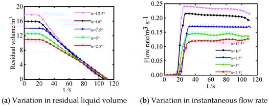
Figure 10.
Variation in residual liquid volume and flow rate with inner wall inclination angle α(Vc = 70% Vcapacity).
No matter how large α is, the residual liquid volume and the flow rate have the same trend. The residual liquid volume first remains unchanged and then decreases to zero, while the flow rate first is zero and then sharply increases to a nearly constant value. As α increases, the initial liquid volume Vc also increases, which directly influences the change curve of the residual liquid volume. Both the initial volume and the flow rate of the liquid steel increase with the increase in α. When α is in the range of 2.5° and 7.5°, the flow rate fluctuates, and when α is in the range of 7.5° and 12.5°, the flow rate slightly decreases. However, when α = 7.5°, the flow rate curve is constant and stable. Therefore, to achieve a stable pouring process and a constant flow rate value, a proper inner wall inclination angle α should be selected in actual production.
3.4. Influence of Initial Liquid Volume Vc
Constant flow rate pouring at different initial liquid volumes Vc is simulated and change curves of the residual liquid volume and the instantaneous flow rate are obtained, as shown in Figure 11. No matter how large Vc is, the residual liquid volume and the flow rate have the same trend. The residual liquid volume first remains unchanged and then decreases to zero, while the flow rate first is zero and then sharply increases to a nearly constant value. As Vc increases, the initial volume, the residual liquid volume, and the flow rate of the steel liquid increase. Except for when Vc = 70% Vcapacity, the flow rate first slightly decreases and then obviously decreases before pouring completion. However, when Vc = 70% Vcapacity, the flow rate curve is constant and stable. Therefore, to achieve a stable pouring process and a constant flow rate value, a proper initial liquid volume Vc should be selected in actual production.
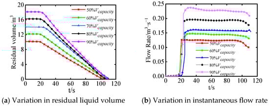
Figure 11.
Variation in residual liquid volume and flow rate with different initial liquid volume (α = 7.5°).
3.5. Influence of Target Flow Rate qt
As different target flow rate qt requires different ladle angular velocity, constant flow rate pouring at different target flow rate qt is simulated and change curves of the residual liquid volume and the instantaneous flow rate are obtained, as shown in Figure 12.
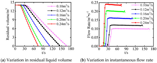
Figure 12.
Variation in residual liquid volume and flow rate at different target flow rates qt (α = 7.5°, Vc = 70% Vcapacity).
No matter how large qt is, the residual liquid volume and the flow rate have the same trend. The residual liquid volume first remains unchanged and then decreases to zero, while the flow rate first is zero and then sharply increases to a nearly constant value. As qt increases, the initial volume remains unchanged, the flow rate of the steel liquid increases, the residual liquid volume decreases more sharply, and the total pouring duration decreases. When qt is in the range of 0.10 m3/s and 0.12 m3/s, the flow rate curve is constant and stable. However, when qt is in the range of 0.16 m3/s and 0.24 m3/s, the flow rate slightly decreases. Therefore, to achieve a stable pouring process and a constant flow rate value, a proper target flow rate qt should be selected in actual production.
4. Experimental Setup and Verification
4.1. Experimental Setup
Liquid steel is of high cost and safety risk, so water is selected as an alternative fluid to verify the pouring process. The water model experiment is based on the Fraude similarity criterion to ensure that the gravity-dominated flow is similar to the dynamics of molten steel. The dynamic viscosity difference is evaluated using the Reynolds number Re. In this study, the Reynolds number Re > 105. Under turbulent conditions, the influence of viscosity can be ignored. Therefore, in the steel liquid pouring simulation, the water pouring experiment can be used to verify the flow behavior of the steel liquid instead of the steel liquid pouring experiment [16]. To verify the accuracy of the analytical model and the simulation model, an experimental setup is constructed, as shown in Figure 13. It consists of many components, including profiles, motors, PLCs, binocular cameras, pressure sensors, circuit breakers, fixed pulleys, pouring ladles, liquid collection buckets, and wire ropes.
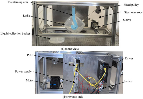
Figure 13.
Overall structure of the experimental setup.
The liquid collection bucket is used to collect the poured liquid, and the residual liquid volume is used to verify the analytical model and the simulation model.
A ladle with an inner wall inclination angle of 7.5° is selected. In the constant flow rate pouring experiments, the motor operates at a pre-set speed and then drives the ladle rotating at a time-variant angular velocity, so precise control of the motor speed is crucial to ensure the constant flow rate.
4.2. Different Initial Liquid Volumes
Three sets of constant flow rate pouring experiments are conducted at the initial liquid volume Vc = 3.90 L, 4.50 L, and 5.10 L, which are about 60%, 70%, and 80% of the total liquid volume, respectively. The target flow rate qt is set to 50 cm3/s. The experimental residual liquid volume is acquired and then compared with that calculated by the analytical model and the simulation model, as shown in Figure 14.
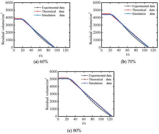
Figure 14.
Comparison at different initial liquid volumes.
It is observed that the experimental results agree well with the theoretical and simulation results at different initial liquid volumes, which verifies the accuracy of the analytical model and the simulation model. Furthermore, the experimental residual liquid volume changes approximately linearly, indicating that the constant flow rate pouring is realized and a constant flow rate can be acquired by adjusting the motor speed.
4.3. Different Target Flow Rates
Three sets of constant flow rate pouring experiments were conducted at the target flow rates qt = 50 cm3/s, 45 cm3/s, and 40 cm3/s. The initial liquid volume Vc is set to 4.5 L, which is about 70% of the total ladle volume. The experimental residual liquid volume is acquired and then compared with that calculated by the analytical model and the simulation model, as shown in Figure 15.
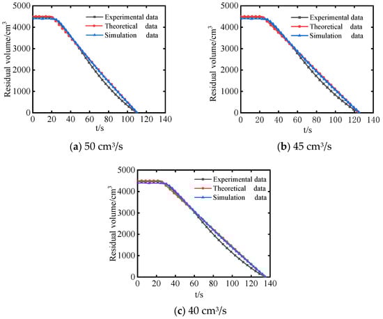
Figure 15.
Comparison at different target flow rates.
It is observed that the experimental results agree well with the theoretical and simulation results at different target flow rates, which verifies the accuracy of the analytical model and the simulation model. Furthermore, the experimental residual liquid volume changes approximately linearly, indicating that the constant flow rate pouring is realized and different constant flow rates can be acquired by adjusting the motor speed.
5. Conclusions
To realize accurate ladle pouring, an analytical model of the constant flow rate pouring was established. By integrating a user-defined function (UDF), a CFD simulation model of the constant flow rate pouring was conducted to investigate the liquid steel pouring behavior under different inner wall inclination angles α, initial liquid volumes Vc, and target flow rates qt. Finally, the accuracy of the analytical model and the simulation model was verified through experiments. The results are as follows:
- (1)
- The experimental results agree well with the theoretical and simulation results, which verify the accuracy of the analytical model and the simulation model.
- (2)
- During the pouring process, the residual liquid volume and the flow rate have the same trend. The residual liquid volume first remains unchanged and then decreases to zero, while the flow rate first is zero and then sharply increases to a nearly constant value.
- (3)
- Increasing both α and Vc leads to an increase in the flow rate. To achieve a stable pouring process and a constant flow rate value, proper α, Vc, and qt should be selected. In this study α = 7.5°, Vc = 70% Vcapacity and q in the range of 0.10–0.12 m3/s are proper.
- (4)
- To realize constant flow rate pouring, a time-variant ladle angular velocity is obtained, and it can be adjusted by the motor speed. Therefore, different constant flow rates could be acquired by adjusting the motor speed, which provides guidance to the engineering application of casting technology.
Author Contributions
Conceptualization, Y.C. and W.Y.; methodology, G.Z. and H.C.; software, Z.H. and C.Q.; validation, G.Z. and H.C.; investigation, Y.C. and W.Y.; data curation, W.Y.; writing—original draft preparation, Z.H. and C.Q.; writing—review and editing, Z.H. and C.Q.; supervision, Y.C. and W.Y.; project administration, G.Z. and H.C.; funding acquisition, Z.H. and C.Q. All authors have read and agreed to the published version of the manuscript.
Funding
This research was funded by the Key Scientific and Technological Project of Henan Province (242102320183), the Key Scientific and Technological Project of the education department of Henan Province (23A470016), the Key Research and Development Project of Henan Province (221111220600) and the Science and Technology Project of Transportation Department of Henan Province (2023-1-2).
Data Availability Statement
The original contributions presented in this study are included in the article. Further inquiries can be directed to the corresponding author.
Conflicts of Interest
Author Hua Chai was employed by the Zheng Machinery (Zheng Zhou) Transmission Technology Co., Ltd. The remaining authors declare that the research was conducted in the absence of any commercial or financial relationships that could be construed as a potential conflict of interest.
References
- Li, C.; Xu, A.; Liu, X. Research progress on several key technologies of converter steelmaking. Steelmaking 2024, 40, 1–8. (In Chinese) [Google Scholar]
- Wang, Y.; Yang, G.; Wang, Y. Converter steelmaking process design and production based on green steel. Iron Steel 2022, 57, 77–86. (In Chinese) [Google Scholar]
- Wang, X. Outlook on progress of steelmaking technology in transition period of Chinese steel industry. Steelmaking 2019, 35, 1–11. (In Chinese) [Google Scholar]
- Alekseenko, S.V.; Antipin, V.A.; Bobylev, A.V.; Markovich, D.M. Application of PIV to velocity measurements in a liquid film flowing down an inclined cylinder. Exp. Fluids 2007, 43, 197–207. [Google Scholar] [CrossRef]
- Cheng, L.; Yu, X.; Deng, X. Research on Pneumatic Quantitative Pouring System by Simulation Experiment. Hot Work. Technol. 2014, 43, 76–78. [Google Scholar]
- Wang, Y.; Miao, L. Automatic Pouring System for Metal Casting based on Learning from Examples. Foundry Technol. 2010, 31, 1503–1506. [Google Scholar]
- Chen, G.; Ma, X.; Wang, C. Current Development of Quantitative Pouring in Casting Production. Foundry Technol. 2015, 11, 56. [Google Scholar]
- He, K.; Xia, Z.; Si, Y.; Lu, Q.; Peng, Y. Noise Reduction of Welding Crack AE Signal Based on EMD and Wavelet Packet. Sensors 2020, 20, 761. [Google Scholar] [CrossRef] [PubMed]
- Wei, M.; Cui, H.; Zhang, H. Study on Flow Field of Thermal Plume during Pouring Process of Molten Iron. Hot Work. Technol. 2017, 46, 114–118+121. [Google Scholar]
- Han, H.; Chen, J.; Yu, H. Modeling and CFD simulation of molten iron pouring process. Mach. Des. Manuf. Eng. 2024, 53, 33–38. [Google Scholar]
- Jin, K. The Research of Hydraulic and Control Technology of Die Casting under Constant Flow Rate Dumping Pouring. Master’s Thesis, Central South University, Changsha, China.
- Nobutoshi, K.; Yoshiyuki, N. Model-Based Flow Rate Control with Online Model Parameters Identification in Automatic Pouring Machine. Robotics 2021, 10, 39. [Google Scholar] [CrossRef]
- Lian, C. The Simulate and Optimize Study on Pneumatic Quantitative Pouring System. Master’s Thesis, North University of China, Taiyuan, China, 2014. [Google Scholar]
- Gao, Q.; Chen, J.; Ji, Y.; Liu, J.; Song, Y. The edge extraction method of casting images based on improved Canny operator. In Proceedings of the 2022 IEEE International Conference on Mechatronics and Automation (ICMA), Guilin, China, 7–9 August 2022; pp. 1708–1713. [Google Scholar]
- Wang, Y. Parameterized Research on New Series Trolleys of Casting Cranes. Master’s Thesis, Taiyuan University of Science and Technology, Taiyuan, China, 2019. [Google Scholar]
- Long, L. Research on Key Technology of Pouring Robot in High Temperature Working Environment. Master’s Thesis, Nanjing University of Aeronautics and Astronautics, Nanjing, China, 2020. [Google Scholar]
Disclaimer/Publisher’s Note: The statements, opinions and data contained in all publications are solely those of the individual author(s) and contributor(s) and not of MDPI and/or the editor(s). MDPI and/or the editor(s) disclaim responsibility for any injury to people or property resulting from any ideas, methods, instructions or products referred to in the content. |
© 2025 by the authors. Licensee MDPI, Basel, Switzerland. This article is an open access article distributed under the terms and conditions of the Creative Commons Attribution (CC BY) license (https://creativecommons.org/licenses/by/4.0/).