Abstract
The accurate prediction of carbon dioxide (CO2) adsorption in metal–organic frameworks (MOFs) is critical for accelerating the discovery of high-performance materials for post-combustion carbon capture. Experimental screening of MOFs is often costly and time-consuming, creating a strong incentive to develop reliable data-driven models. Despite extensive research, most studies rely on standalone models or generic ensemble strategies that fall short in handling the complex, nonlinear relationships inherent in adsorption data. In this study, a novel ensemble learning framework is developed by integrating five distinct regression algorithms: Random Forest, XGBoost, LightGBM, Support Vector Regression, and Multi-Layer Perceptron. These algorithms are combined into four custom ensemble strategies: equal-weighted voting, performance-weighted voting, stacking, and manual blending. A dataset comprising 1212 experimentally validated MOF entries with input descriptors including BET surface area, pore volume, pressure, temperature, and metal center is used to train and evaluate the models. The stacking ensemble yields the highest performance, with an R2 of 0.9833, an RMSE of 1.0016, and an MAE of 0.6630 on the test set. Model reliability is further confirmed through residual diagnostics, prediction intervals, and permutation importance, revealing pressure and temperature to be the most influential features. Ablation analysis highlights the complementary role of all base models, particularly Random Forest and LightGBM, in boosting ensemble performance. This study demonstrates that custom ensemble learning strategies not only improve predictive accuracy but also enhance model interpretability, offering a scalable and cost-effective tool for guiding experimental MOF design.
1. Introduction
The rising atmospheric concentration of carbon dioxide (CO2) is a primary driver of global climate change and remains one of the most critical environmental concerns worldwide. Industrialization, fossil-fuel combustion, and deforestation have all contributed significantly to increased CO2 emissions, prompting urgent efforts to deploy carbon capture, utilization, and storage (CCUS) technologies as part of decarbonization strategies [1,2]. Among the various CCUS technologies, post-combustion carbon capture is particularly promising because of its adaptability to existing infrastructure and energy systems [3,4]. Conventional chemical adsorption systems, particularly those based on alkanolamines, are energy-intensive and corrosive, and their long-term application faces issues of solvent degradation and environmental toxicity [5,6]. These limitations have led to a shift toward physical adsorption processes using porous materials, which offer improved cyclic stability and regeneration efficiency [1,7]. Among these, metal–organic frameworks (MOFs) have emerged as frontrunners due to their ultrahigh surface areas, chemically tunable functionalities, and flexible framework topologies [6,8].
MOFs are crystalline structures composed of metal ions coordinated to organic ligands, which form periodic porous networks with tailorable pore environments. Their structural diversity allows for the design of adsorption sites specific to CO2, enabling high selectivity even at low partial pressures [9,10]. Thousands of MOFs have been synthesized and thousands more computationally generated, but their comprehensive evaluation using laboratory or molecular simulation methods remains time- and resource-intensive [1,3]. As such, the application of machine learning (ML) to predict CO2 uptake in MOFs has become increasingly essential in accelerating materials discovery and screening.
ML approaches are well suited to capturing the non-linear, multi-dimensional relationships between structural descriptors and adsorption performance. Regression algorithms such as Random Forest, Support Vector Regression, and Gradient Boosting Machines have been widely employed to predict CO2 uptake capacities using physicochemical and topological descriptors such as surface area, pore volume, electronegativity, and void fraction [1,5,6]. These descriptors are often extracted using tools such as Zeo++ and then provide a standardized basis for model development [3,11,12].
Recent studies have reported high predictive accuracies using ensemble learning models trained on curated adsorption datasets. Longe et al. [6] developed a robust machine learning framework using multiple-feature-selection techniques and ensemble models, achieving high correlation coefficients and low error metrics across test sets. Similarly, Li et al. [1] applied Random Forest and XGBoost to experimental CO2-uptake data and reported improved accuracy over single-model approaches. Both studies emphasized the importance of model interpretability and the need for consistent feature scaling and selection. Amar et al. [7] proposed a smart ensemble scheme using Gradient Boosting and Random Forest models, demonstrating improved prediction stability and generalizability. Their study incorporated SHapley Additive exPlanations (SHAP) to analyze the contribution of each feature, revealing that volumetric descriptors, polarizability, and pore-surface heterogeneity were among the most influential variables. Similarly, Achour & Hosni [5] used permutation importance to quantify the effects of features on model performance and highlighted the predictive strength of open metal sites and topological surface area. Despite these advances, most ensemble applications rely on off-the-shelf configurations without integrating complementary model types. This creates an opportunity to explore custom ensemble frameworks that combine linear and non-linear regressors, potentially improving prediction across diverse data distributions and descriptor sets [3,12]. Approaches that blend strategies that merge predictions from heterogeneous base learners have shown potential in other materials domains but remain underexplored in the context of MOF-based CO2 capture [6,7]. Although ensemble learning has demonstrated considerable potential in improving predictive performance in MOF-based CO2 adsorption modeling, existing studies often apply standard ensemble configurations without tailoring them to the specific statistical and structural complexities of MOF datasets. This limitation reduces the adaptability of such models, particularly in contexts involving mixed types of descriptors and non-uniform data distributions across adsorption regimes. Moreover, the combined use of algorithmically distinct learners, such as decision tree ensembles, kernel-based regressors, and neural networks, within a single unified predictive system remains insufficiently explored in the current literature.
To address these research gaps, the present study developed and evaluated multiple custom ensemble learning models designed to enhance prediction accuracy and generalizability for CO2 uptake in MOFs. The ensemble configurations integrated five distinct base learners: Random Forest, Extreme Gradient Boosting (XGBoost), Light Gradient Boosting Machine (LightGBM), Support Vector Regression (SVR) optimized through grid search, and a Multi-Layer Perceptron (MLP) regressor. These base models were combined using multiple ensemble strategies, including equal-weighted voting, performance-weighted voting based on inverse root mean square error, and stacking with Ridge regression as the meta-learner. All models were trained and validated using standardized experimental data composed of key MOF descriptors, including surface area, pore volume, pressure, temperature, and metal identity. The performance of the ensemble models was rigorously assessed using multiple-regression metrics, such as coefficient of determination (R2), root mean square error (RMSE) and mean absolute error (MAE). Also, an analysis comparing our best-performing ensemble model with those from other published studies was performed. Furthermore, advanced diagnostics including residual analysis, an ablation study, and a regression characteristic curve were applied. Other analysis such as permutation-based feature importance and William’s plot was applied to identify key predictive features and interpret model behavior. Through the design and evaluation of these custom ensemble models, this study contributes a robust and scalable framework for improving the predictive accuracy and interpretability of data-driven CO2-capture screening.
2. Materials and Methods
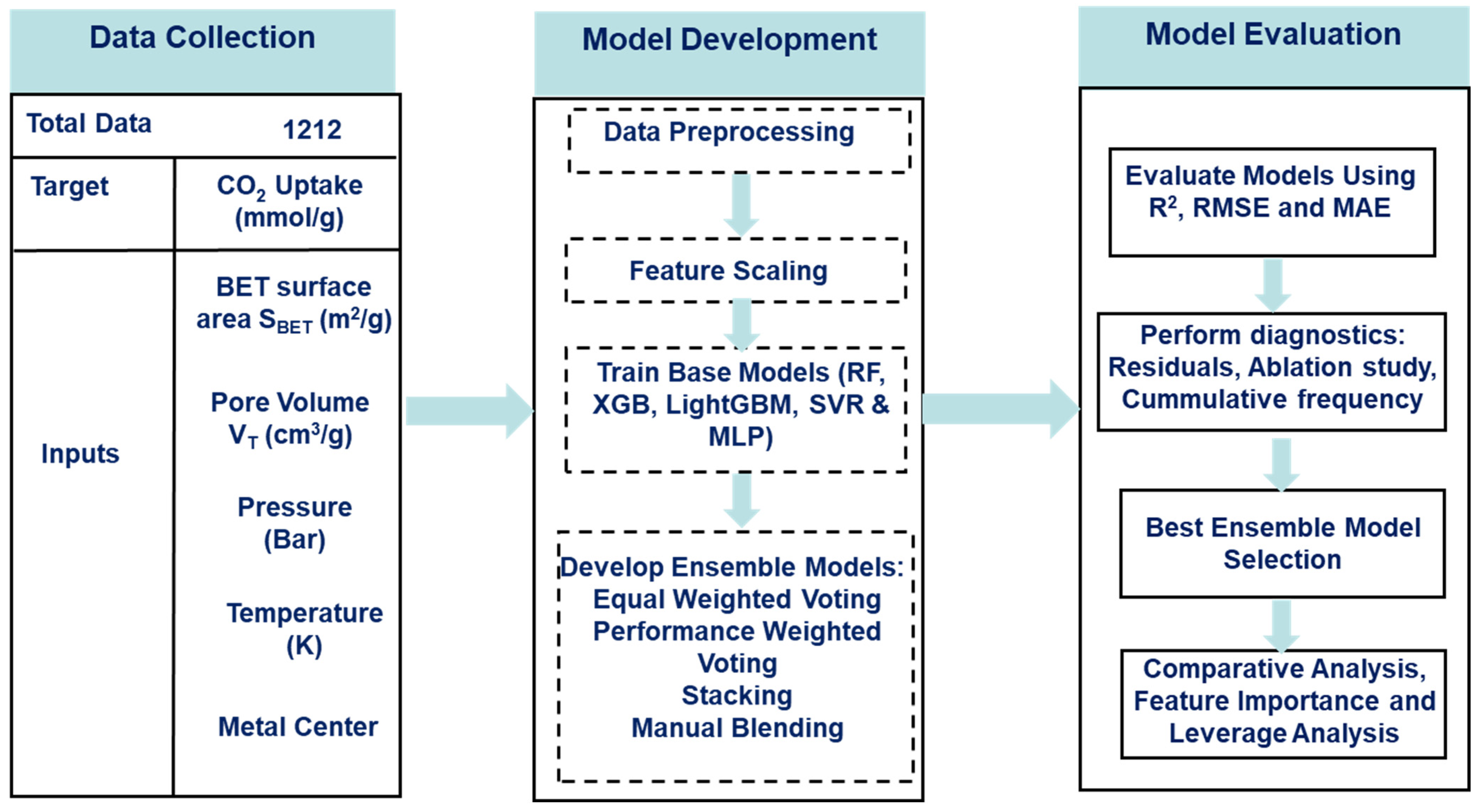
This section of the report showcases the materials, namely the data, the data-driven algorithm, and the software used for executing it, as well as the methodology involved in obtaining the models from the algorithms. Additionally, the methodology for training and tuning the algorithms and combining the algorithms into ensemble structures is described in detail. Figure 1 provides a schematic overview of the methodological workflow adopted in this study, illustrating the sequence of processes from data preprocessing to model evaluation.

Figure 1.
Workflow for CO2-uptake prediction.
2.1. Data Collection and Description
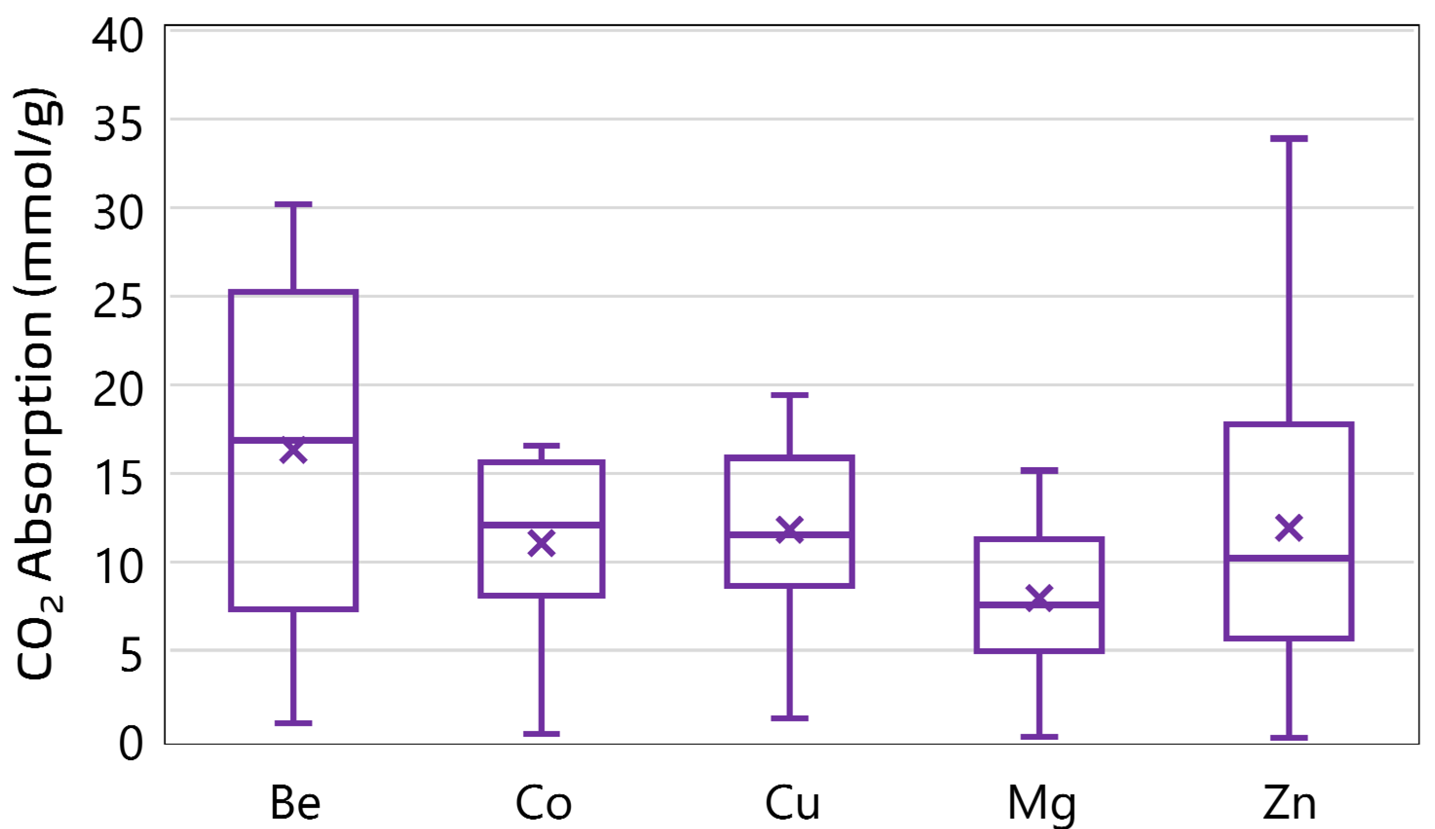
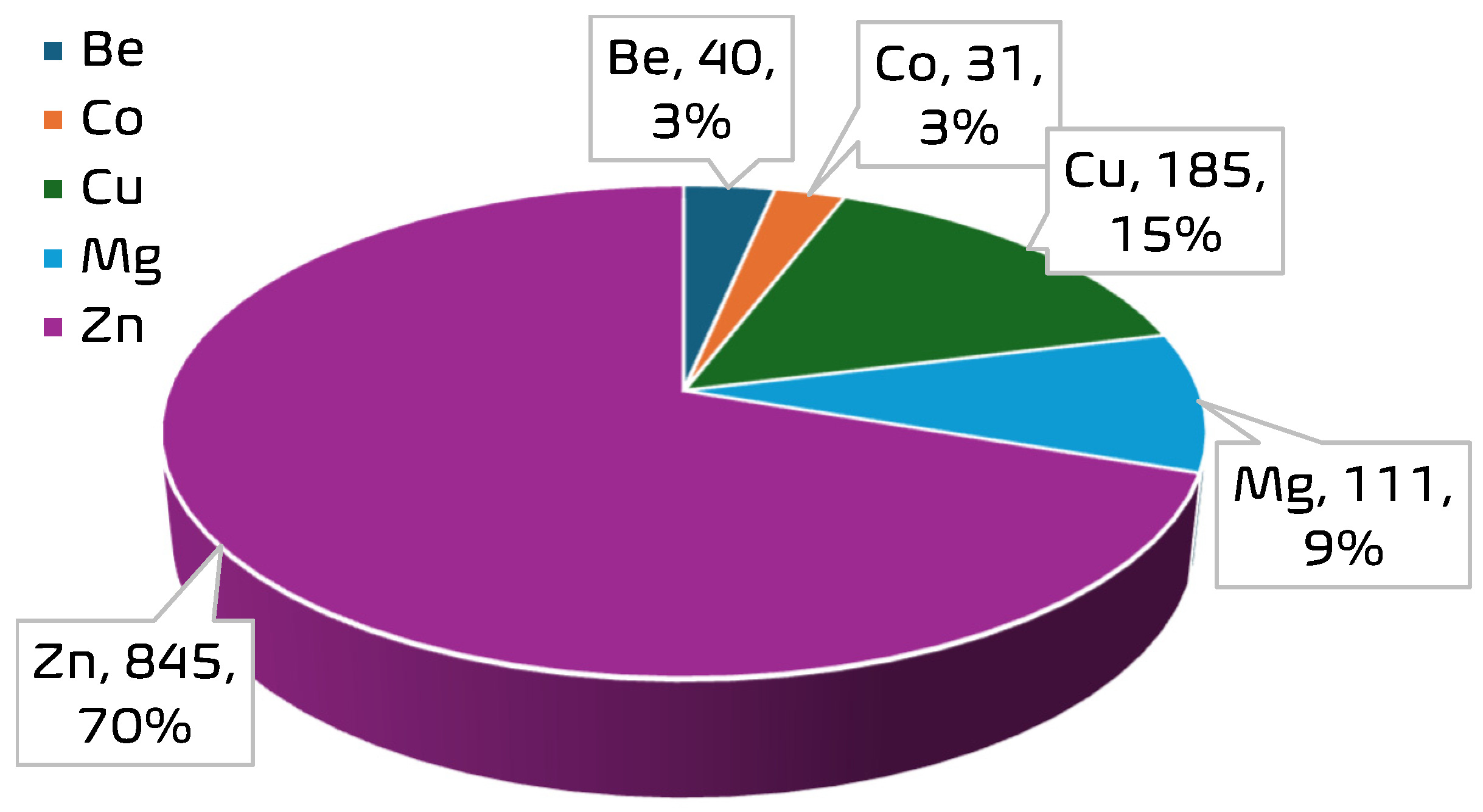
A curated experimental dataset comprising 1212 data points was compiled to support the development of ensemble machine learning models for predicting CO2 uptake in metal–organic frameworks (MOFs). The dataset aggregates CO2-adsorption measurements obtained under varying thermodynamic conditions across a range of MOF structures with distinct metal centers. Each data point corresponds to a unique combination of operational parameters and structural descriptors extracted from validated literature sources [10,13,14]. The dataset encompasses a diverse range of MOF structures. A total of 35 unique MOF samples are represented, with the most frequently occurring materials being MOF-5 (149 entries), PCN-11 (117), HKUST (112), PCN-16 (105), and ZIF-8 (100). The dominance of these materials suggests a focus in the literature on well-studied MOF architectures known for high porosity and thermal stability. In terms of metal distribution, the dataset is strongly skewed toward Zn-based frameworks, which account for 845 data points; Zn is followed in frequency by Cu (185), Mg (111), Be (40), and Co (31). See Figure 2 and Figure 3 for the distribution of the metal centers in the datasets. This distribution reflects an experimental emphasis on zinc-centered MOFs, particularly on Zn-MOF-74 and MOF-5, due to their established adsorption capabilities and structural robustness. The presence of Be- and Co-based frameworks, though limited in quantity, provides additional diversity in the metal-node chemistry, enabling broader generalizability of the predictive models. The input variables are pressure (P), temperature (T), Brunauer–Emmett–Teller surface area (SBET), pore volume (VT), and metal center (MC), while CO2-adsorption capacity was the target variable. Table 1 presents a statistical summary of the numerical features in the dataset, including their minimum, maximum, mean, and standard deviation. These descriptors formed the foundation for feature engineering and model development in subsequent stages of this study.
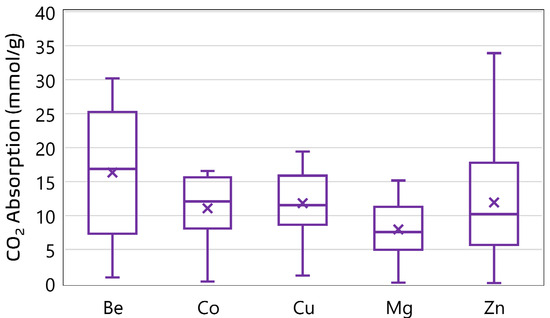
Figure 2.
CO2-adsorption performance of MOFs with different metal ions.

Figure 3.
Frequency of metal centers in the MOF dataset.

Table 1.
Statistical description of features.
The metal center (MC), a categorical variable that represents the elemental identity of the inorganic node in an MOF structure, significantly influences the adsorption behavior of CO2 due to its impact on surface charge, pore geometry, and strength of interaction with gas molecules [7,10]. Prior studies have shown that variations in metal species can affect the heat of adsorption, framework stability, and CO2 selectivity [1,5]. To enable its inclusion in numerical modeling, the “metal center” variable was label-encoded into distinct integer classes. Specifically, the five observed metal types (Zn, Cu, Mg, Be, and Co) were mapped to integer values ranging from 0 to 4. This label encoding preserved categorical differentiation without imposing ordinal relationships. The encoded variable was subsequently used as a predictive feature in all machine learning models, allowing the algorithms to capture compositional trends across MOF variants with diverse metal centers [3,8].
2.2. Model Development
This section outlines the modeling framework adopted for developing the ensemble models. The process begins with preprocessing of the dataset to ensure consistency and compatibility with model requirements, and this step is followed by feature scaling to normalize the input space. A diverse set of base models comprising tree-based, kernel-based, and neural network architectures were developed to capture the complex non-linear relationships between MOF descriptors and CO2-adsorption capacity. To enhance predictive robustness and leverage complementary strengths of individual algorithms, multiple ensemble strategies were employed. These included equal-weighted voting, performance-weighted voting based on inverse error, stacking with a meta-learner, and a manual blending strategy. The pipeline was designed to systematically train, evaluate, and integrate these models using rigorous validation and interpretability tools. The following subsections provide detailed descriptions of each stage in the model-development process, beginning with data preprocessing.
2.2.1. Data Preprocessing
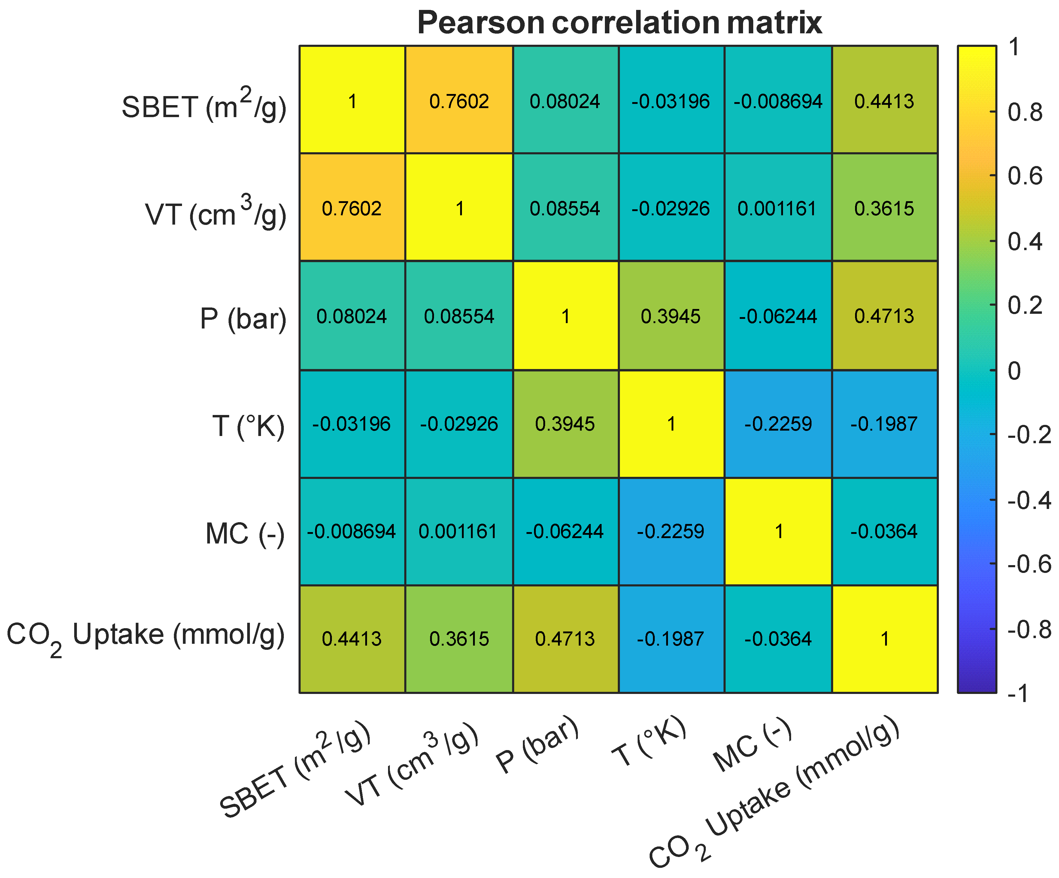
As an initial step in model development, a correlation analysis was conducted to examine the pairwise linear relationships between the input variables and the target variable, CO2 uptake (mmol/g). Figure 4 presents the Pearson correlation matrix for all numerical features in the dataset, including BET surface area (SBET), total pore volume (VT), pressure (P), temperature (T), and the encoded metal center (MC). Among the predictors, pressure showed the strongest positive correlation with CO2 uptake (r = 0.47), followed by BET surface area (r = 0.44) and total pore volume (r = 0.36). These results align with prior findings that elevated pressure enhances gas adsorption by increasing the driving force for diffusion and interaction at adsorption sites [1,3,15]. The relevance of SBET and VT in adsorption modeling is also well established, as they are indicative of the available surface area and accessible pore volume for gas diffusion [5,7,9]. A strong inter-correlation between SBET and VT (r = 0.76) was observed, which is consistent with previous reports describing the interplay between pore-size distribution and total surface area in high-capacity adsorbents [16,17]. In contrast, temperature exhibited a weak negative correlation with CO2 uptake (r = −0.20), which is consistent with the exothermic nature of physisorption processes and has been highlighted in prior thermodynamic studies [6,18]. The encoded “metal center” variable also showed a weak correlation with the target (r = −0.04), but prior work emphasizes that while label encoding may not capture nuanced chemical properties directly, its inclusion can still enhance model performance by signaling key compositional differences [8,19].
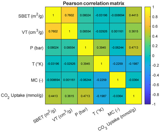
Figure 4.
Pearson correlation heatmap of input features and the target variable.
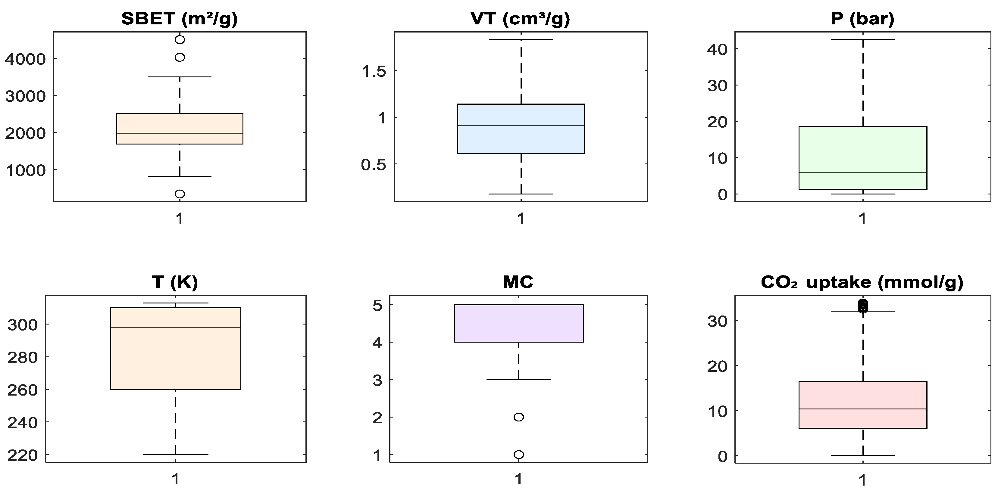
Despite these observed correlations, no input feature demonstrated multicollinearity levels that warranted exclusion. All variables were retained to allow machine learning algorithms, especially those capable of capturing non-linear interactions, such as tree-based models, to fully explore feature relationships. Subsequent steps involved standardizing the data to align the input space for algorithms sensitive to feature scaling. Figure 5 presents boxplots for all features used in model development. These plots were used to assess the central tendency, spread, and presence of outliers in the dataset prior to modeling. Several features, including SBET, P, and CO2 uptake, included visible outliers, particularly on the upper tail of their distributions. In the case of CO2 uptake, a few samples exceeded 30 mmol/g, while SBET included values above 4000 m2/g. These high-value outliers are consistent with literature findings in which certain MOFs exhibit exceptional surface area or adsorption capacity under optimized conditions [3,6,7]. However, to reduce model bias and stabilize learning algorithms sensitive to skewed distributions, extreme outliers were removed during preprocessing. This decision was guided by the need to balance data integrity with model generalizability, as the inclusion of extreme values may disproportionately influence weights in a regression model [5,12]. For the metal center (MC), which was label-encoded as an integer feature, the boxplot indicates limited spread, with a few outliers representing rare metal types. These were retained to preserve class diversity during model training. The boxplot analysis justified selective outlier removal to ensure robust and consistent model performance.
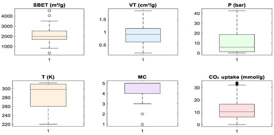
Figure 5.
Boxplot visualization of input features and target variable.
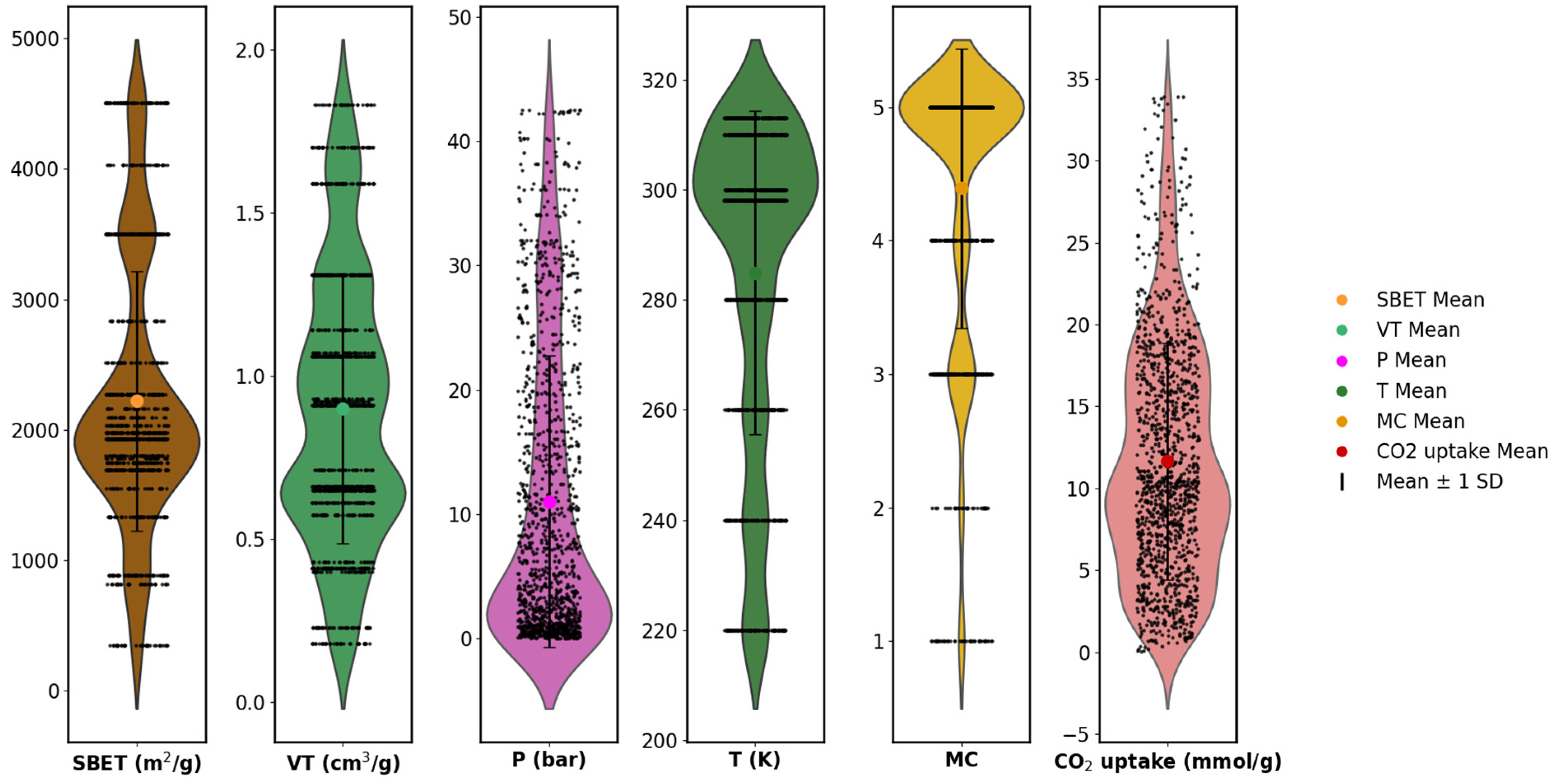
To complement the boxplot analysis, violin plots were generated for all numerical features to further examine the underlying distributions. As shown in Figure 6, the features exhibited varying degrees of skewness, kurtosis, and spread. For example, SBET and CO2 uptake had multi-modal and right-skewed distributions, while temperature and pore volume had relatively compact distributions. The encoded metal center (MC), though categorical, showed uneven class frequencies across the range. The presence of distributional asymmetries and differing value ranges across features reinforces the need for normalization before model training. These observations provide quantitative justification for the use of feature scaling, especially when employing models that are sensitive to input magnitudes and distribution shapes [1,5,15,20].

Figure 6.
Violin plots show the probability density distribution of features.
2.2.2. Feature Scaling
Following data cleaning and exploratory analysis, feature scaling was applied to normalize the range of numerical input variables and prepare the dataset for training. Scaling is a critical preprocessing step for many machine learning algorithms that are sensitive to the magnitude of feature values, particularly those that rely on distance metrics or gradient-based optimization, such as Support Vector Regression (SVR) and Multi-Layer Perceptron (MLP) neural networks [1,6]. In this study, the StandardScaler from the scikit-learn library was employed to standardize the input features by removing the mean and scaling to unit variance. This transformation ensures that each feature contributes equally to the learning process, thereby improving convergence speed and model stability, especially for ensemble techniques that integrate both scale-sensitive and scale-invariant models [3,8]. Categorical variables such as the label-encoded metal center were excluded from this transformation to preserve their numerical identity. All feature scaling was performed using parameters learned exclusively from the training subset to avoid data leakage. The same transformation was then applied to the test subset using the fitted scaler. This process ensured consistency and reproducibility across model-evaluation phases.
2.2.3. ML Algorithms
In the model-development stage, five distinct regression algorithms were employed as base learners to capture various patterns within the dataset: Random Forest (RF), Extreme Gradient Boosting (XGBoost), Light Gradient Boosting Machine (LightGBM), Support Vector Regression (SVR), and Multi-Layer Perceptron (MLP). This selection was motivated by their complementary learning capabilities: ensemble trees are adept at handling non-linear relationships and interactions among features, while SVR and MLP are capable of capturing complex functional mappings in high-dimensional spaces [21,22,23]. To ensure comprehensive representation of both non-linear dependencies and latent feature interactions within the adsorption dataset, each model was carefully selected based on its theoretical strengths and proven effectiveness in similar domains. The following subsections describe the fundamental principles and operational mechanisms of the individual regression algorithms employed, including their mathematical foundations, learning strategies, and suitability for the task of CO2-uptake prediction.
Random Forest Regressor
Random Forest (RF) is an ensemble-based supervised learning method that operates by constructing a multitude of decision trees during training and outputting the mean prediction of each of the individual trees for regression tasks. It mitigates overfitting by introducing randomness through bootstrap aggregation (bagging) and random feature selection at each split [24].
Let represent the kth decision tree trained on a bootstrapped dataset with random feature selection, where denotes the random vector governing the tree’s structure. The RF output is the average over all M trees, as follows:
RF models are robust to noise and collinearity and are particularly well-suited for non-linear relationships, as has been observed in MOF datasets [5,12].
Extreme Gradient Boosting (XGBoost)
XGBoost is a highly efficient and scalable implementation of gradient-boosted decision trees introduced by [25]. It uses additive model construction with second-order Taylor approximation and incorporates regularization to reduce overfitting.
where F is the space of regression trees and denotes each tree. The objective function minimized by XGBoost is as follows:
where L is a differentiable loss function, Ω(f) is a regularization term, T is the number of leaves, and Wj are the leaf weights.
Light Gradient-Boosting Machine (LightGBM)
LightGBM is a gradient-boosting framework optimized for efficiency and scalability. It employs a histogram-based algorithm and leaf-wise tree growth, which significantly accelerates training while maintaining accuracy [26]. In a departure from the level-wise growth used in traditional GBDTs, LightGBM grows trees by choosing the leaf with the highest loss reduction, as follows:
This leads to the creation of deeper trees and better generalizability on complex datasets. Additionally, LightGBM handles categorical features directly and implements techniques like Gradient-based One-Side Sampling (GOSS) and Exclusive Feature Bundling (EFB) to improve computational performance.
Support Vector Regression (SVR)
SVR applies the principles of Support Vector Machines to regression, aiming to find a function f(x) that deviates from the true response y by no more than ϵ for each training point and that is as flat as possible. The function has the following form:
Here, and are slack variables representing the deviation of training samples outside the ε-insensitive margin and C is the regularization parameter that controls the trade-off between model complexity and tolerance to deviations beyond ε. The RBF kernel is commonly used in SVR to map inputs into higher-dimensional spaces, enhancing non-linear modeling capacity [3,9].
Multi-Layer Perceptron (MLP) Regressor
MLP is a feedforward artificial neural network composed of an input layer, one or more hidden layers with non-linear activation functions, and an output layer. For regression, the network learns a mapping = f(x; θ), where θ denotes weights and biases optimized via backpropagation. A typical forward pass through one hidden layer takes the following form:
where φ is the activation function. MLPs are powerful universal function approximators capable of modeling highly non-linear patterns in multidimensional descriptor spaces [5,8].
z(1) = W(1)x + b(1),
a(1) = φ(z(1))
2.2.4. Ensemble Learning
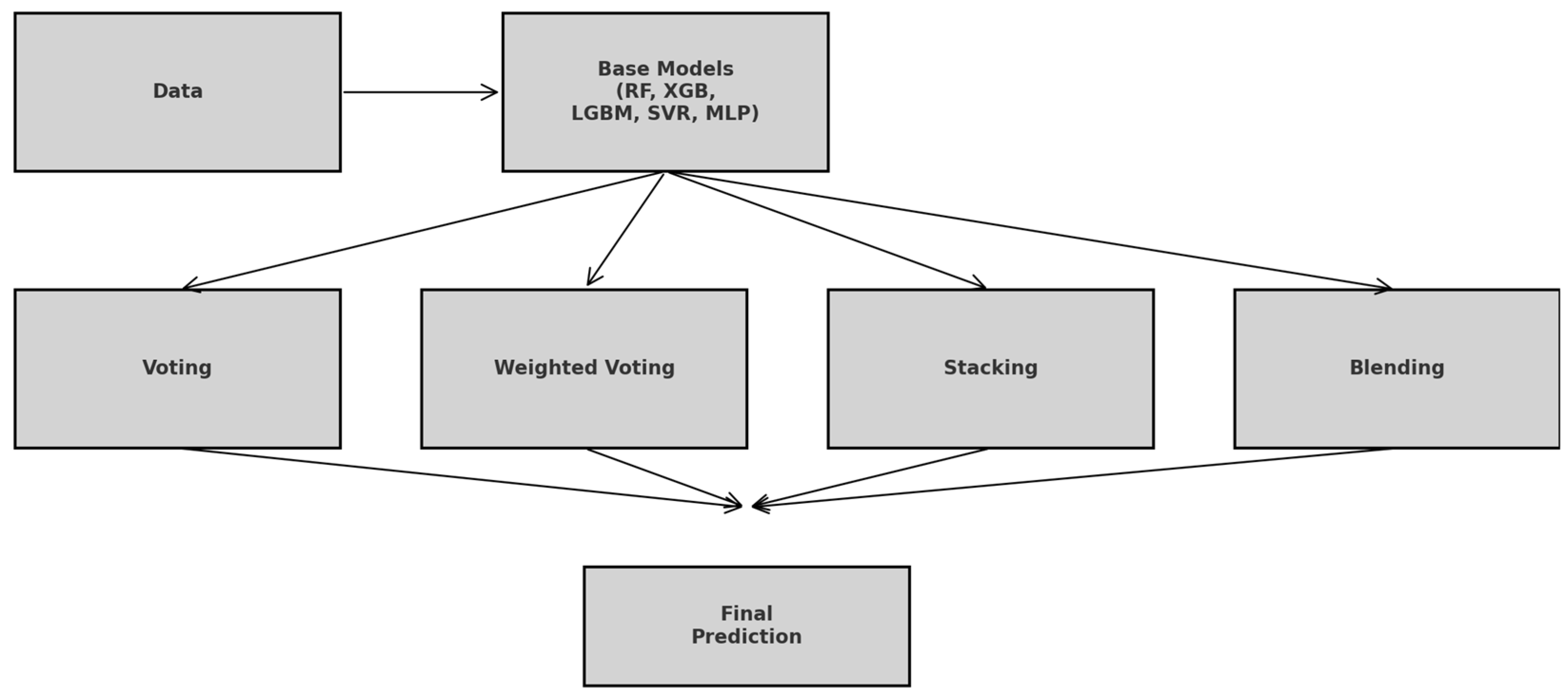
Ensemble learning refers to a class of machine learning techniques in which multiple base models are strategically combined to produce a more robust and generalizable predictive model. The underlying principle is that by aggregating the strengths of diverse learners, the ensemble can reduce variance, mitigate bias, and improve predictive performance beyond what individual models can achieve [27,28]. This approach is particularly effective for complex, non-linear regression tasks, such as the prediction of CO2 uptake in structurally diverse MOFs, where different algorithms may excel in capturing different aspects of data distribution. In this study, four ensemble learning strategies were explored: equal-weighted voting, performance-weighted voting, stacking, and manual blending. Figure 7 illustrates the simplified workflow showing how the raw data feed into each of the five base learners, branch into equal-weighted voting, performance-weighted voting, stacking, and manual blending, and then recombine into the final prediction.
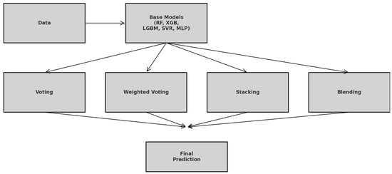
Figure 7.
Ensemble Learning Workflow: From Base Learners to Final Prediction.
Equal-Weighted Voting Ensemble
Equal-weighted voting is one of the simplest ensemble strategies for regression tasks, but it is nonetheless effective. In this approach, predictions from multiple base learners are averaged without assigning any preference or weight to individual model performance [29]. If denotes the prediction of the ith base model, then the final ensemble prediction is computed as follows:
where n is the total number of base models. This method assumes that all models contribute equally to the final prediction and that their individual biases can cancel each other out. While it is simplistic, equal-weighted averaging has been shown to yield competitive performance in various regression settings, especially when the base models are sufficiently diverse [7,30,31]. In this study, predictions from five base regressors (Random Forest, XGBoost, LightGBM, SVR, and MLP) were aggregated using equal-weighted voting. This ensemble provided a performance benchmark for assessing the contribution of each model when the models were treated as equally reliable. The results obtained from this strategy were further compared to weighted and stacked approaches to evaluate the impact of model-specific influence.
Weighted Voting Ensemble
Weighted voting extends the equal-weighted ensemble approach by assigning different weights to each base learner based on their predictive performance. This strategy assumes that not all models contribute equally to the final prediction; instead, models with superior accuracy should have greater influence in the ensemble output [22,32]. For a set of n base regressors, the ensemble prediction is computed as follows:
where is the prediction of the ith model, and wi is the corresponding weight such that In this study, weights were derived based on the inverse of each model’s root mean squared error (RMSE) on the validation set, as follows:
This formulation ensures that models with lower prediction error (i.e., higher accuracy) are assigned greater influence. Weighted ensembles have been found to reduce variance and bias more effectively than simple averaging, particularly in regression problems involving heterogeneous learners [29,33,34].
Stacking Ensemble
Stacking ensemble learning, also referred to as stacked generalization, is a meta-learning technique that integrates predictions from multiple base models using a secondary learning algorithm (meta-learner) to produce a final output. Unlike bagging or boosting, which rely on homogeneous learners and iterative learning strategies, stacking allows the combination of heterogeneous base learners, enabling it to leverage diverse learning patterns across models [34,35]. For this study, stacking was implemented by training the five base regressors on the same training dataset. The predictions from these base learners were then used as input features to train a meta-regressor, specifically Ridge regression, on a hold-out validation set. This architecture enables the meta-learner to discover optimal combinations of base-model outputs that minimize prediction error on unseen data [12,21]. Mathematically, the stacking prediction stack can be represented as follows:
where is the prediction from the i-th base model and is the function learned by the meta-learner. This framework capitalizes on the individual strengths of each model, e.g., tree ensembles for capturing non-linearity and support vector machines for high-dimensional margin optimization, resulting in a more robust predictor [36]. The efficacy of stacking for tasks in materials informatics, particularly MOF-based gas separation and adsorption, has been recently demonstrated by [23], who employed a stacking ensemble to screen polymer–MOF membranes.
Manual Blending Ensemble Learning
Manual blending is a variant of ensemble learning that combines the strengths of multiple base learners by training a meta-model on their individual predictions. Unlike traditional stacking methods, which often rely on K-fold cross-validation to generate out-of-fold predictions, manual blending adopts a simpler, two-stage data-partitioning strategy [28]. In this approach, the training set is explicitly split into two subsets: the first (referred to as Set A) is used to train the base models, and the second (Set B) is used to generate their predictions, which in turn serve as input features for training a meta-learner. Let the original training data be represented by Xtrain and Ytrain. These are partitioned into two subsets: XA, yA and XB, yB, such that the following holds:
Base learners f1, f2, …, fn are first trained on (XA, yA). Their predictions on XB form a new feature matrix Z Rmxn, where each column Zi corresponds to the predictions of model fi on XB. The meta model g, typically a linear regressor, is then trained on (Z, yB), yielding the final ensemble function, as follows:
The five regressors utilized in this study were selected as base learners due to their complementary strengths in handling non-linearity, high dimensionality, and multicollinearity. The Ridge regressor was used as the meta-learner owing to its ability to mitigate overfitting via L2 regularization [37].
2.3. Model Evaluation
The performance of the developed machine learning models and ensemble systems was assessed using three key regression-evaluation metrics: mean absolute error (MAE), root mean squared error (RMSE), and the coefficient of determination (R2). The expressions of these statistical metrics are defined in Equations (19)–(21). These metrics are commonly used in machine learning studies to evaluate model accuracy, consistency, and explanatory power [21,32,38]. RMSE measures the square root of the average squared difference between predicted and actual values. It penalizes larger errors more heavily and is sensitive to outliers. This makes it suitable for detecting significant deviations. MAE calculates the average absolute difference between predicted and actual values. It is more interpretable and less sensitive to outliers than RMSE, making it useful for understanding general prediction reliability. R2 quantifies the proportion of variance in the target variable that is predictable from the input features. Higher R2 values indicate better model fit and generalizability. These metrics were selected to provide complementary insights into model performance. RMSE captures magnitude-based accuracy; MAE represents overall deviation; and R2 assesses explanatory strength.
The RMSE is given by the following:
and the coefficient of determination, R2, is expressed as follows:
3. Results
This section presents the predictive performance, robustness, and comparative analysis of the developed machine learning models for CO2 adsorption in MOFs under carbon-capture conditions.
3.1. Tuning of Hyperparameters
Hyperparameter tuning is essential during model-building to improve the model’s performance and predictive accuracy. Hyperparameter tuning involves systematically testing a range of values to find the optimal settings for each parameter. This process ensures that the model is neither overfitted nor underfitted, thereby improving its generalizability to new, unseen data. This study explored various hyperparameter ranges to identify the best configurations for all models. Table 2 presents the optimal hyperparameter values determined through this rigorous tuning process.
Table 2.
Hyperparameter tuning for ML models..
3.2. Performance of Ensemble Models
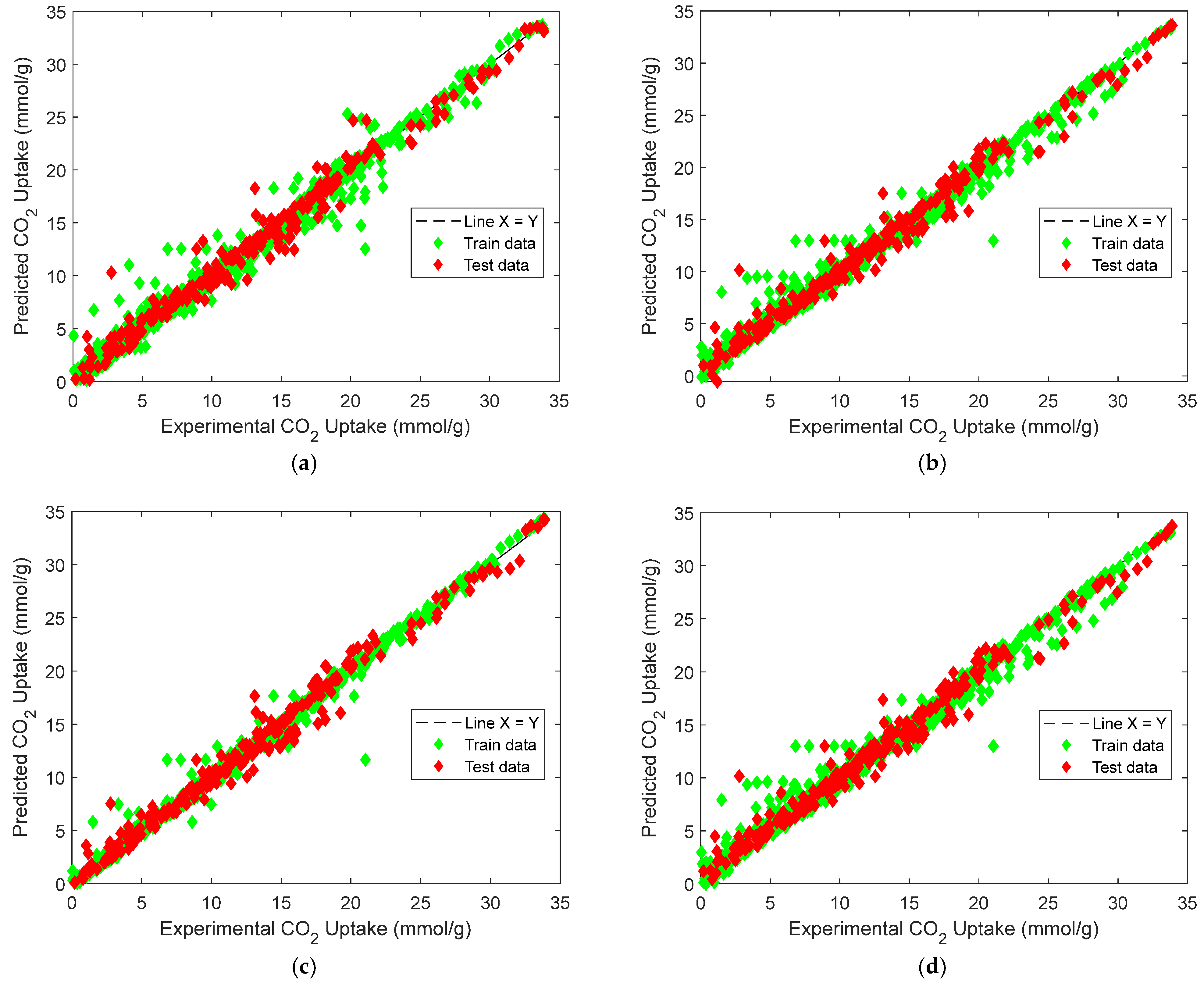
The final features used to develop the models include SBET, VT, P, T, and MC, as shown in Figure 1 The machine learning workflow developed in this study involved the training and evaluation of both individual base learners and ensemble models with these features to predict CO2 uptake in metal–organic frameworks (MOFs). The base models served as foundational learners from which four ensemble learning strategies were subsequently constructed: equal-weighted voting, weighted voting, stacking, and manual blending. Each ensemble model aimed to integrate the strengths of the individual learners while minimizing their limitations. Figure 8 illustrates the parity plots for the ensemble models, comparing the predicted and experimental CO2-uptake values across the training and test sets. The X = Y reference line indicates perfect prediction accuracy, and the clustering of points around this line provides a visual validation of model reliability. Table 3 summarizes the performance metrics of each base learner in terms of R2, RMSE, and MAE.

Figure 8.
Predicted vs. experimental CO2 uptake: (a) manual blending, (b) weighted voting, (c) stacking, (d) equal-weighted voting.
Table 3.
Comparison of models’ performance metrics.
Figure 8 depicts the predicted versus experimental CO2-uptake values for the four ensemble models. Each subplot includes predictions on both the training and test sets, which are plotted against the ideal X = Y reference line to visualize predictive alignment. Across all four ensembles, the points are closely clustered along the diagonal, indicating strong predictive agreement. The stacking regressor [Figure 8c] shows the closest alignment with the X = Y line, confirming its superior performance in minimizing prediction error, a result consistent with the quantitative metrics reported earlier. The weighted voting model [Figure 8b] also demonstrates robust generalizability, with predictions evenly distributed across low and high uptake values. In contrast, the equal-weighted voting model [Figure 8d] shows slightly increased deviation, particularly at higher adsorption values, likely due to its uniform treatment of all base learners regardless of individual accuracy. The manual blending ensemble [Figure 8a] also tracks the true values well, though minor scatter is visible in mid-range predictions.s
Table 3 provides a detailed performance evaluation of both base and ensemble learning models using training and test data. Among the base models, XGBoost demonstrated the highest generalizability, with a test R2 of 0.9747, an RMSE of 1.2339, and MAE of 0.7628, indicating strong accuracy and minimal overfitting. Random Forest also performed well, with a test R2 of 0.9639, offering a good balance between interpretability and predictive strength. Although LightGBM achieved a decent R2 of 0.9562, its relatively higher RMSE (1.6222) and MAE (1.0809) suggest it was less precise on certain test samples. On the other hand, SVR and MLP exhibited comparatively lower test performance, with R2 values of 0.9316 and 0.8916, respectively. Their elevated RMSE and MAE values indicate higher sensitivity to outliers and potentially limited generalizability across the full range of CO2 uptake.
In contrast, the ensemble models consistently outperformed the individual learners. The Stacking ensemble achieved the best overall metrics, with an R2 of 0.9833, an RMSE of 1.0016, and an MAE of 0.6630, confirming the effectiveness of meta-learning in combining diverse model predictions. The equal-weighted voting and weighted voting ensembles also performed strongly, with R2 scores of 0.9792 and 0.9779, respectively. Notably, weighted voting achieved lower test errors (RMSE: 1.1527, MAE: 0.7558) than its equal counterpart, reflecting the value of incorporating model-specific performance weights. Finally, the manual blending model produced competitive results, with an R2 of 0.9765 and an MAE of 0.7429, though its RMSE of 1.1889 was slightly higher than that of the stacking model.
To verify that the ensemble performance on our held-out test set was not an artifact of a particular split, we conducted five-fold cross-validation on the full dataset. Each ensemble was wrapped in a scaling pipeline so that feature standardization occurred inside every fold. Table 4 reports the mean and standard deviation of R2, RMSE and MAE across the five folds.
Table 4.
Five-fold CV results for the models.
The cross-validation results reveal a clear hierarchy among the standalone learners and demonstrate the value of combining models. Among the individual regressors, the tree-based methods lead the pack, with the highest baseline predictive accuracy and the tightest fold-to-fold consistency. In contrast, support-vector regression exhibits noticeably lower explanatory power and greater variability, while the multilayer perceptron occupies an intermediate position, offering moderate accuracy but larger error spreads than the tree ensembles.
Introducing ensemble schemes improves both accuracy and robustness across every metric. All four ensemble approaches outperform their single-model counterparts, confirming that diverse learners capture complementary information. Stacking delivers the most accurate and stable predictions and is closely followed by weighted voting. Equal-weight voting and manual blending also yield substantial gains over the base learners, though they show slightly greater variability. The marked reduction in cross-fold standard deviations for the ensemble methods underlines how combining models produces more reliable performance on unseen splits.
4. Discussion
4.1. Analysis of Residual Error
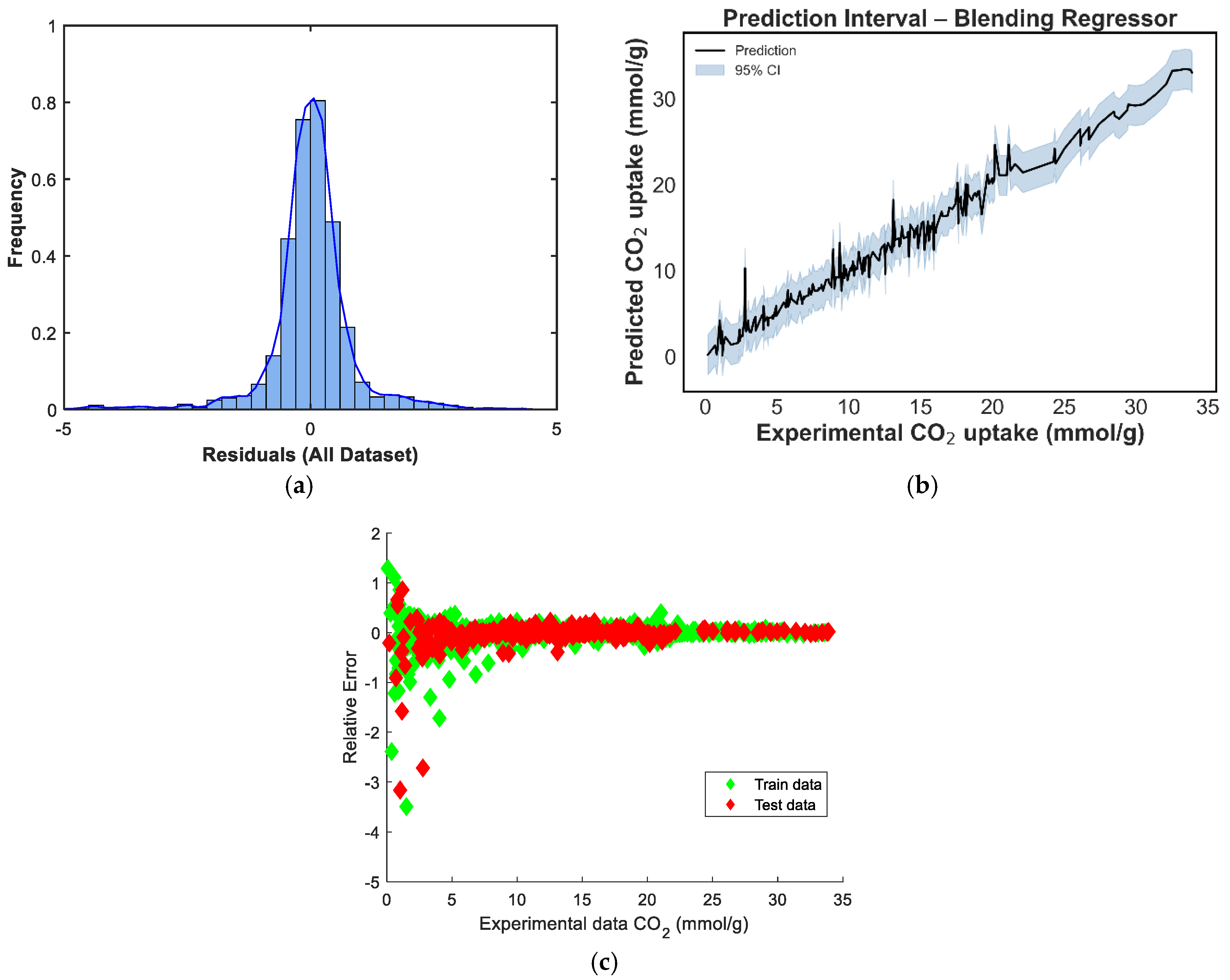
To provide deeper insights into the internal behavior and reliability of the ensemble models, several diagnostic analyses were conducted. These include prediction-interval plots, residual-distribution histograms, and scatterplots of residuals versus predicted valuescatterplot. Such analyses help assess not only the accuracy but also the consistency and stability of each model’s predictions across the range of CO2-uptake values. The prediction-interval plots visualize the uncertainty bounds surrounding the model predictions, offering a sense of confidence in the estimates for both low- and high-uptake regions [39]. Residual histograms provide a statistical overview of model bias and error dispersion, helping to identify deviations from normality or the presence of outliers. Meanwhile, plots of residuals versus predicted value serve as diagnostic tools for detecting heteroscedasticity, systematic error patterns, or model underfitting, with random scatter indicating a well-calibrated model and patterned deviations suggesting structural inadequacies [40]. Figure 9, Figure 10, Figure 11, and Figure 12 show the diagnostic plots for each of the ensemble models, respectively.

Figure 9.
Prediction diagnostics for the manual blending regressor: (a) residual distribution, (b) 95% prediction interval, and (c) residuals vs. experimental CO2 uptake.

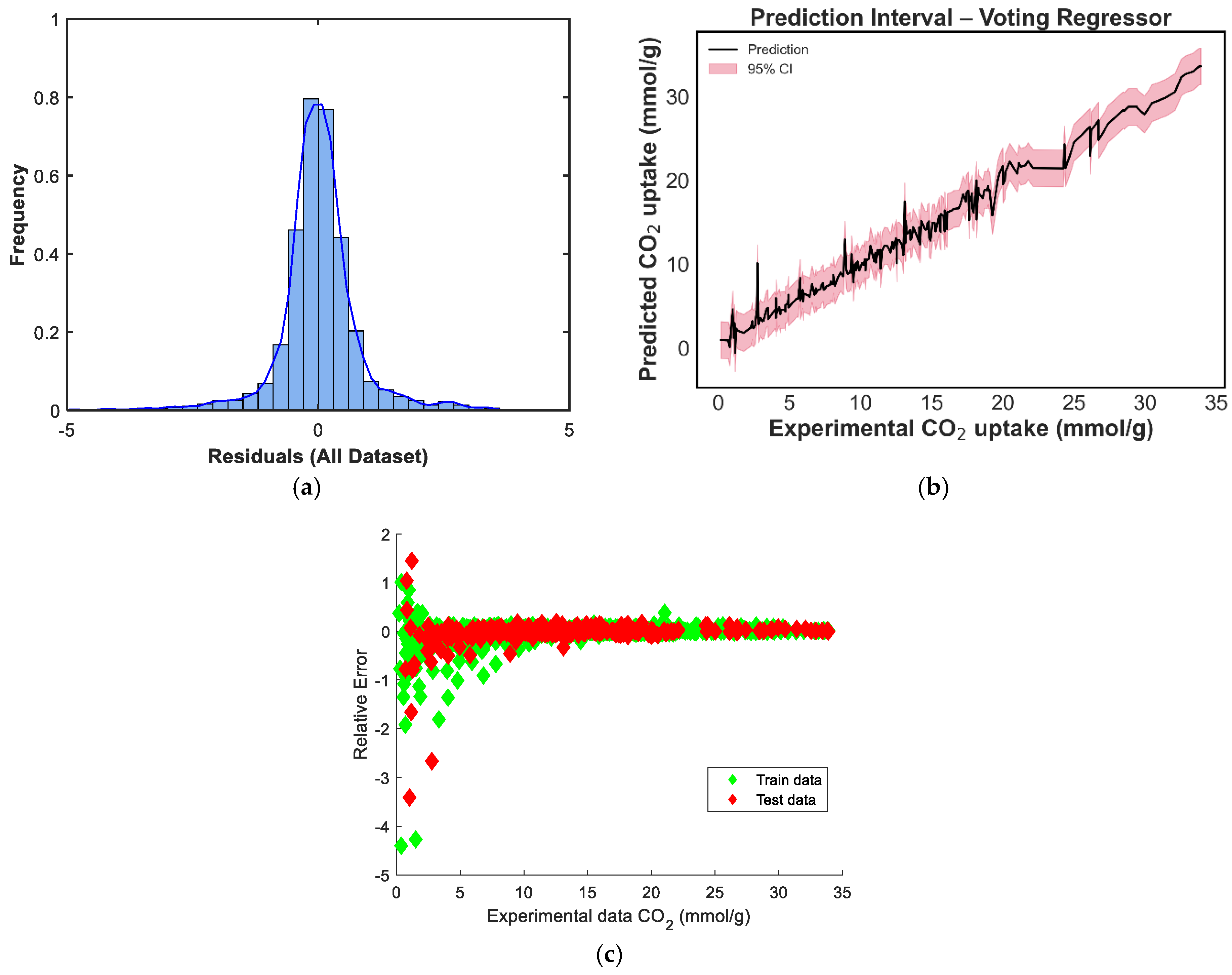
Figure 10.
Prediction diagnostics for the weighted voting regressor: (a) residual distribution, (b) 95% prediction interval, and (c) residuals vs. experimental CO2 uptake.
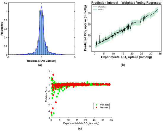
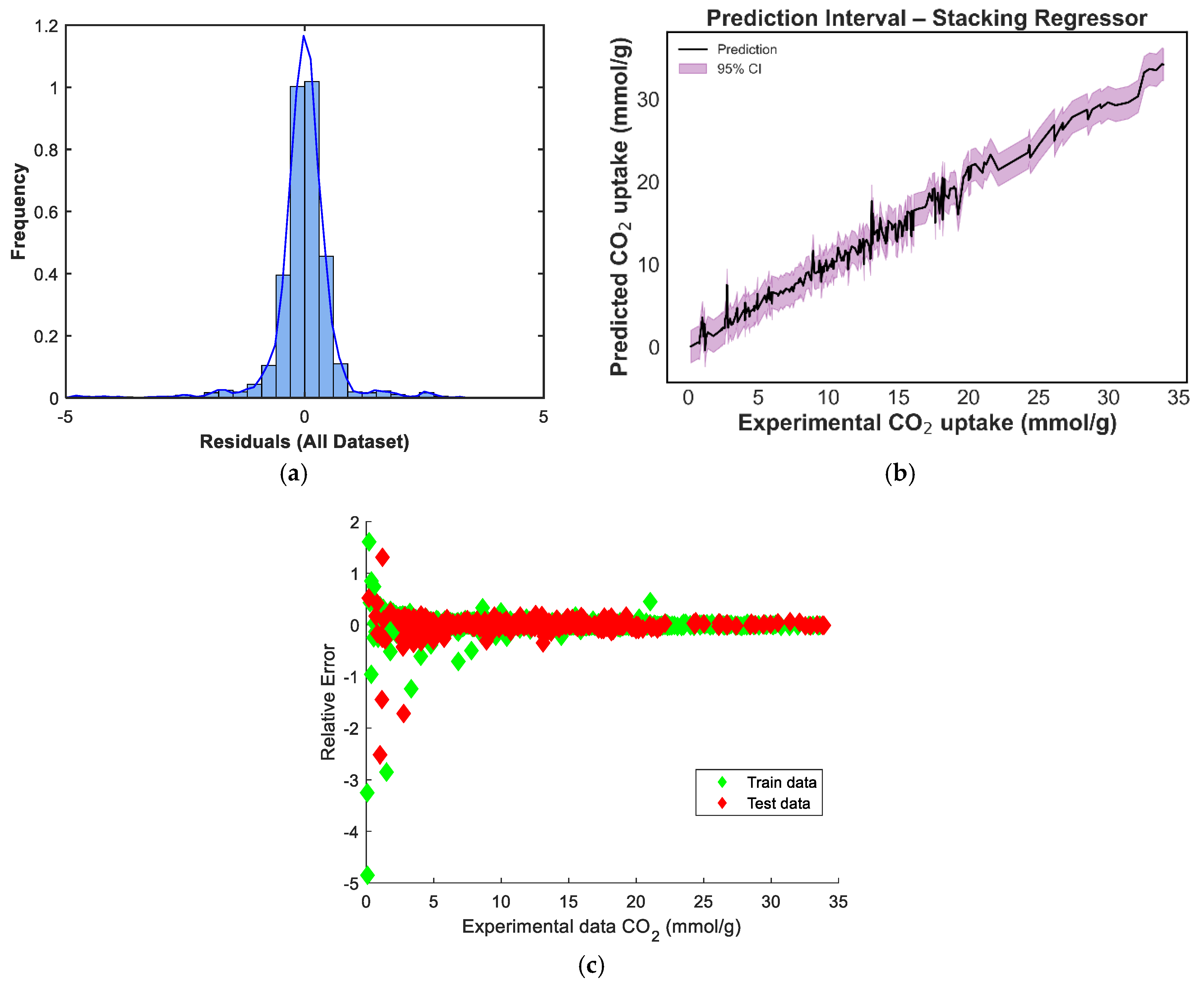
Figure 11.
Prediction diagnostics for the stacking model: (a) residual distribution, (b) 95% prediction interval, and (c) residuals vs. experimental CO2 uptake.

Figure 12.
Prediction diagnostics for the equal weighted voting regressor: (a) residual distribution, (b) 95% prediction interval, and (c) residuals vs. experimental CO2 uptake.
The residual distribution in Figure 9a shows a near-normal shape, with residuals centered around zero, indicating that the model does not exhibit significant bias and that prediction errors are symmetrically distributed. However, a slight left skew and heavier left tail can be observed, suggesting a few under-predictions on the test set. Figure 9b displays the prediction intervals for the blending model across the experimental CO2 uptake range. The narrow spread of the confidence intervals in the mid-range, with slightly widening intervals at the extremes, reflects increased model certainty around the bulk of the data and greater uncertainty in regions with fewer training points [39]. In Figure 9c, the residuals-versus-predicted scatterplot shows no clear trend, confirming the absence of strong heteroscedasticity or systematic error patterns. Most points are distributed tightly around the horizontal zero line, supporting the conclusion that the model generalizes well without systematic over- or under-estimation across prediction magnitudes. The residual distribution in Figure 10a is nearly symmetric, with a sharp peak around zero, indicating that the model has low average bias [40]. However, a minor left tail and some slight kurtosis suggest the presence of a few underpredictions, although these are limited in magnitude. Figure 10b shows the prediction interval for the equal-weighted voting model. The 95% confidence bands appear generally narrow around the mid-range values and slightly wider toward the boundaries, reflecting increased uncertainty where fewer data points are present. This suggests stable performance across the bulk of the data, though some variance persists at extreme levels of CO2 uptake. In Figure 10c, the residuals-versus-predicted plot shows a reasonably uniform spread, with no strong visible trends or curvature, suggesting the model does not suffer from heteroscedasticity. The residuals are more concentrated around the zero line across most of the prediction range, which affirms the voting regressor’s general reliability.
In Figure 11a, the residual distribution is centered around zero and exhibits a slight left skew. Although the shape approximates a normal distribution, the presence of minor negative outliers suggests that the model tends to slightly underpredict in a few instances [40]. The prediction-interval plot in Figure 11b shows a well-bounded 95% confidence range across the prediction domain. The uncertainty bands remain tight across mid-range CO2-uptake values and widen only slightly at the distribution tails, indicating high model stability in regions where data are concentrated [39]. Figure 11c provides a scatterplot of residuals versus predicted values, and the residuals are randomly distributed around the horizontal axis. This pattern implies no evident heteroscedasticity or model bias, confirming that the weighted voting strategy offers robust and unbiased predictions across the range of CO2-uptake values.
The residual histogram in Figure 12a is symmetrical and peaks around zero, closely resembling a normal distribution. This suggests that prediction errors are evenly distributed, with no pronounced bias, and that extreme deviations are rare. Figure 12b illustrates the stacking model’s prediction interval. The confidence bands are consistently tight across the uptake spectrum, indicating stable and reliable predictions. This reflects the ensemble’s ability to maintain low variance while preserving generalizability, especially at high and low CO2-adsorption values, where other models showed slightly wider intervals. In Figure 12c, the residuals-versus-predicted plot confirms this behavior. Residuals are tightly clustered along the zero line, with no discernible pattern, confirming that the stacking model generalizes well and avoids heteroscedasticity or functional drift. This validates its superior performance metrics and reinforces its status as the best-performing ensemble approach in this study.
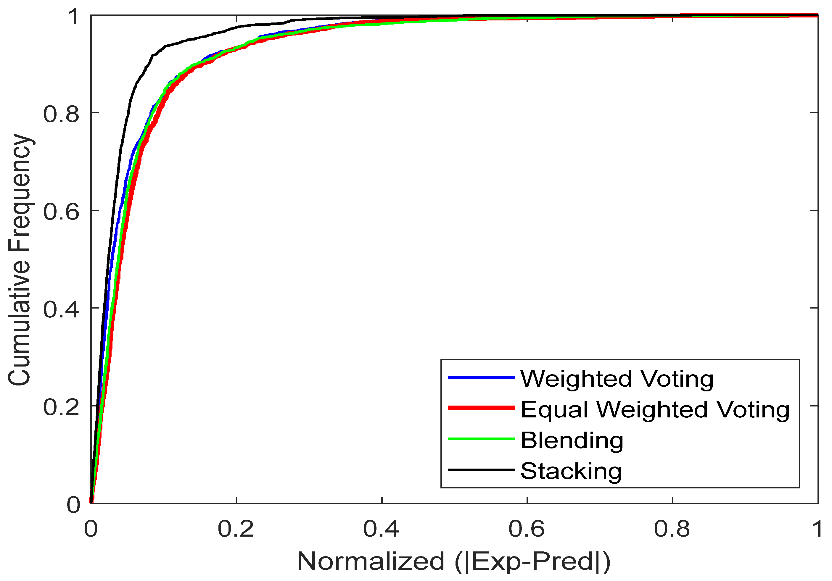
4.2. Cumulative-Frequency Analysis
The cumulative frequency plot in the provided figure serves as an interactive visualization tool to assess the reliability of predictive models. Positions higher and closer to the vertical axis indicate more accurate predictions. The plot includes cumulative frequency curves for manual blending, weighted voting, stacking and equal-weighted voting. From Figure 13, the plot clearly shows that the stacking model outperforms the other ensemble models. The curve for stacking model is nearer to the vertical axis, indicating that the model produces predictions with lower error values for most data points. Conversely, the other ensemble models significant lags, showing a lower cumulative frequency in this error range and indicating more frequent errors of greater magnitude.
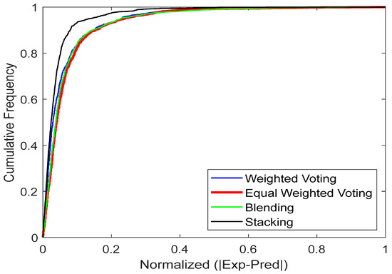
Figure 13.
The models’ cumulative frequency for predicting CO2 uptake in MOFs.
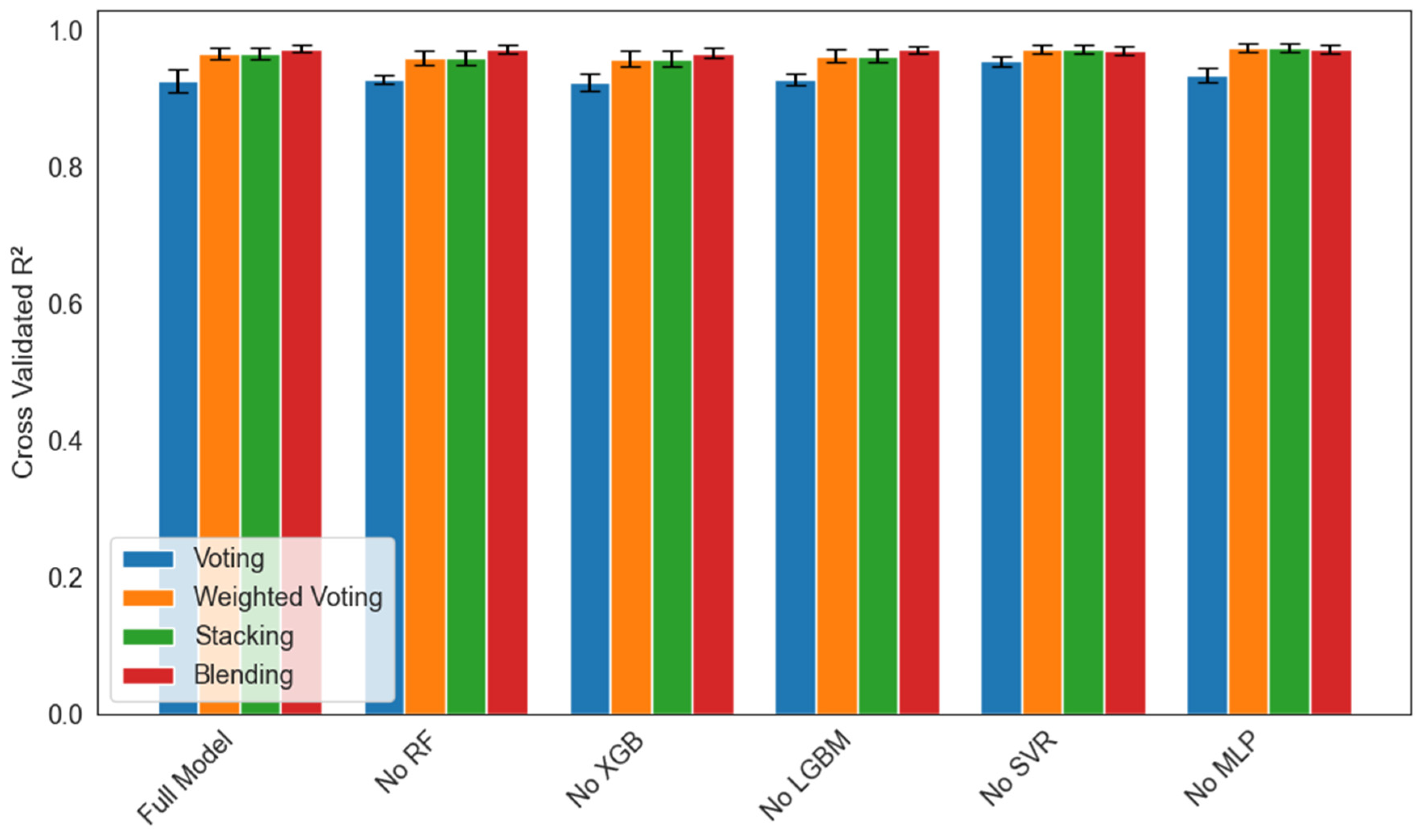
4.3. Ablation Study
An ablation study was performed with five-fold cross-validation to quantify each base learner’s contribution to four ensemble strategies (voting, weighted voting, stacking, and manual blending) under six conditions (full model or a model with Random Forest, XGBoost, LightGBM, SVR, or MLP removed). Figure 14 reports the mean R2 ± 1 SD across folds for each scenario. Removal of Random Forest caused the largest drop in mean R2 (by one to two percentage points) and the greatest fold-to-fold variability in all four ensembles, which underscores RF’s critical role in stabilizing predictions. Excluding XGBoost or LightGBM led to a moderate decrease in mean R2 (0.5 to 1.0 points) and slightly wider error bars, indicating the importance of gradient boosting for capturing nonlinear structure. Omitting SVR or MLP had only a minimal effect on mean R2 (≤0.2 points), with very small standard deviations, suggesting these learners contribute complementary information but are not central to overall accuracy. Across every leave-one-out condition, the stacking regressor consistently achieved the highest mean R2 and the smallest standard deviation, which confirms its superior robustness to individual model perturbations.
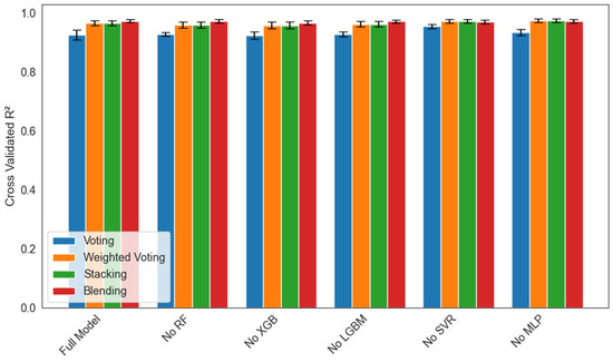
Figure 14.
Ablation study of ensemble models showing mean cross-validated R2 ± 1 SD over five folds for each leave-one-out scenario (Full Model, No RF, No XGB, No LGBM, No SVR, and No MLP) across four ensemble strategies: Voting (blue), Weighted Voting (orange), Stacking (green), and Blending (red).
4.4. Comparative Analysis with Published Studies
To further contextualize the performance and novelty of the proposed custom ensemble learning framework, a comparative analysis was conducted with four recent and relevant studies in the literature that applied machine learning techniques for predicting CO2 adsorption in MOFs. These studies vary in dataset size, feature types, algorithmic strategies, and performance metrics. Table 5 presents a consolidated comparison, highlighting not only model performance (in terms of R2 and RMSE), but also the breadth of features used, the level of interpretability offered, and the computational efficiency of each approach.
Table 5.
Comparative analysis of machine learning models for prediction of CO2 adsorption in MOFs. The assessment of CO2 adsorption in MOFs is based on performance on the test dataset.
As shown in Table 4, while prior studies have made notable contributions to the development of machine learning models for CO2 adsorption in MOFs, the present work contributes marked advancements across several dimensions. The most direct performance gain is observed in the model accuracy, where the proposed ensemble model achieved an R2 of 0.9833, surpassing the best-reported R2 scores in the literature (Longe et al. [6]; R2 = 0.9798 and Abdi et al. [20]; R2 = 0.9733). Despite Longe et al. [6], integrating hybrid ML-optimization schemes, their dataset comprised only 475 entries, significantly fewer than the 1212 MOFs used in this study, which contributes to improved generalizability and model robustness. In contrast to the model developed by Abdi et al. [20], which achieved a high R2 but lacked interpretability due to its black-box GNN structure, this study integrated both accuracy and transparency. The proposed ensemble model incorporates SHAP analysis, permutation importance, residual diagnostics, prediction intervals, and ablation studies, offering a multifaceted view of model behavior and variable contribution. This level of interpretability is not available in most of the referenced studies, where either limited feature-importance plots [7] or basic SHAP summaries [1] are used. Furthermore, this study’s use of custom ensemble strategies (equal and weighted voting, stacking, and blending) distinguishes it from previous models that largely relied on either individual regressors [6,20] or a single stacking framework [7]. By evaluating multiple ensemble configurations and selecting the best based on rigorous diagnostics, the present work ensures model stability and predictive consistency. Additionally, this study achieved a lower RMSE = 1.0016 and MAE = 0.7903 than all previous models with complete metric reporting, indicating not only better fit but also smaller prediction errors. This is particularly noteworthy given that prior studies either do not report MAE ([6,20]) or report higher values [7], such as an MAE of 0.903.
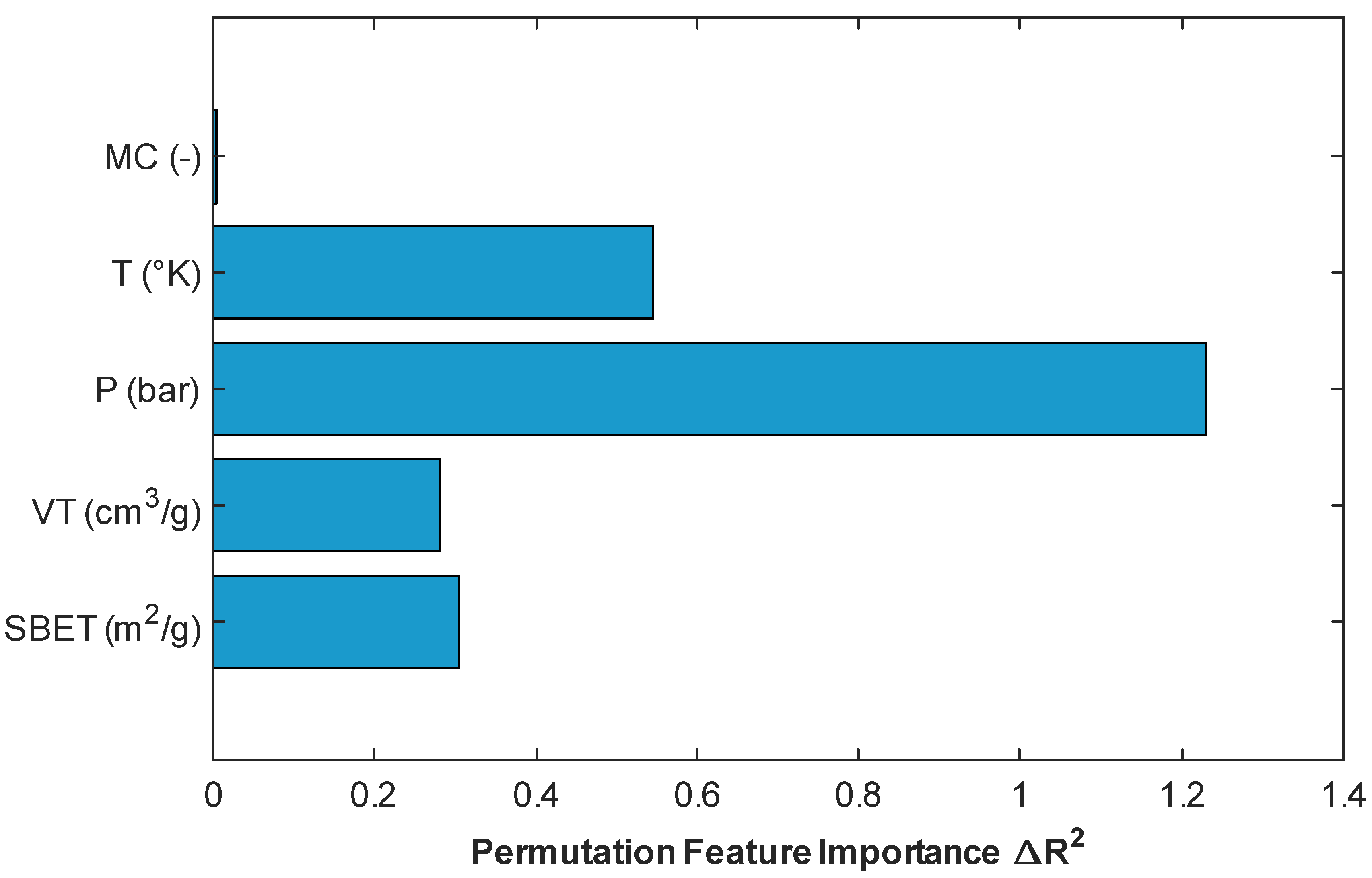
4.5. Permuation Feature Importance
To better understand the contribution of individual input features to the overall model performance, permutation importance analysis was conducted using the stacking regressor, which had demonstrated superior predictive performance. Permutation importance is a model-agnostic interpretability technique that quantifies the impact of each feature by measuring the change in prediction error (ΔR2) when the feature’s values are randomly shuffled, thereby breaking its relationship with the target variable [35]. As illustrated in Figure 15, pressure (P) had the most impact on the model’s performance, with a significant drop in R2 occurring when this variable was perturbed, which confirms its dominant role in determining CO2 uptake. This is consistent with adsorption physics, as pressure directly governs gas–solid interactions and adsorption equilibrium [5,7]. Temperature (T) ranked second in importance, which aligns with its role in influencing adsorption kinetics and thermodynamics [1]. Among the textural properties, BET surface area (SBET) and pore volume (VT) also contributed negatively to model performance, although to a lesser extent than operational parameters. Notably, the “metal center” (MC) variable showed negligible importance in this particular model configuration, suggesting either that its effect is nonlinear and thus not captured through shuffling or that it is redundant given the other features provided. This trend corroborates findings from previous authors [1,2]. These outcomes confirm that pressure and temperature are the most influential descriptors for prediction of CO2 adsorption in MOFs, while surface and structural attributes provide complementary, though less dominant, explanatory power.

Figure 15.
Plot of permutation-based feature importance obtained from the stacking model.
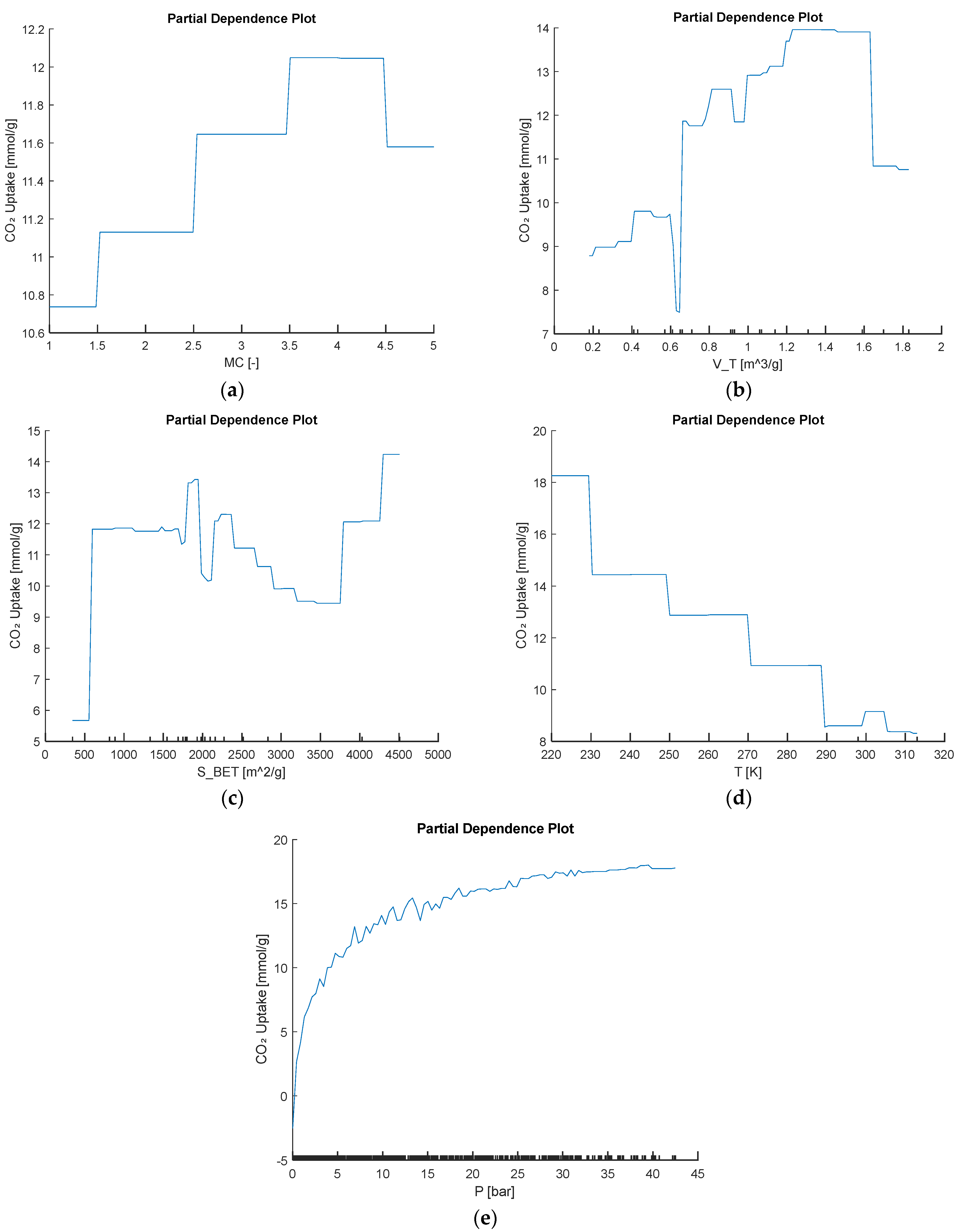
4.6. Partial Dependence Plot
In addition to the global SHAP and permutation-importance results, several complementary interpretability perspectives can be applied to each base model. For tree-based learners, average marginal effects (e.g., partial dependence) reveal how changes in key predictors such as metal center, surface area, and pore volume drive CO2 uptake, exposing nonlinear and saturation behavior. In support-vector regression, analysis of the learned dual coefficients identifies which support vectors lie closest to the regression boundary and thus strongly influence generalizability. In the multilayer perceptron, inspection of input-to-hidden connection-weight magnitudes provides a global feature ranking by net effect on the output. Local surrogate-model methods such as shallow decision trees or local linear approximations can further illustrate how individual feature perturbations drive single-sample predictions. Using the best-performing model, we generated the partial dependence plot in Figure 16 to show the behavior trend of input variables to CO2 uptake.
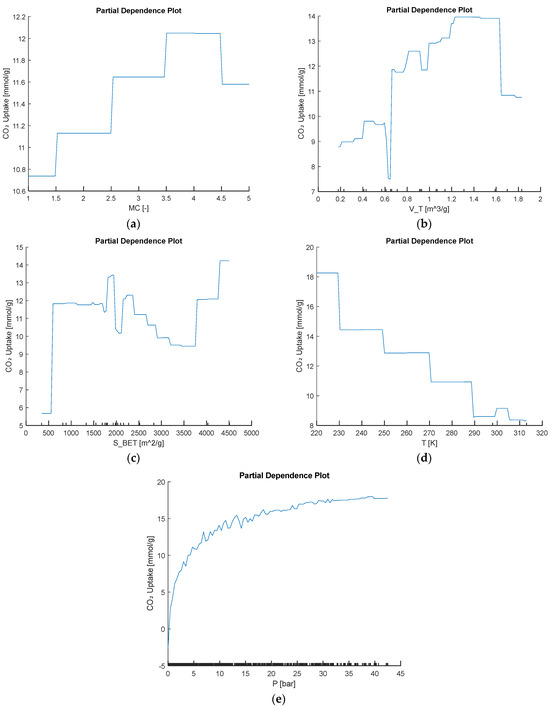
Figure 16.
Partial dependence of predicted CO2 uptake on the input variables (a) MC, (b) VT, (c) SBET, (d) T, and (e) P.
The partial dependence plot for metal center shows that beryllium- and cobalt-based frameworks give the lowest predicted CO2 uptakes. Uptake then jumps sharply for copper- and magnesium-centered materials, reaching a maximum around 12 mmol/g, before dipping slightly for zinc. This clear, stepwise trend illustrates that copper and magnesium generate the most favorable binding sites and underscores how strongly metal identity alone can tune adsorption performance. In addition to metal-center effects, the other dependence curves follow clear, chemistry-driven patterns. As pore volume VT increases, predicted uptake rises almost monotonically from about 9 mmol g−1 at the smallest volumes to nearly 14 mmol g−1 at the largest, reflecting the greater void space for CO2. Surface area SBET shows a similar near-linear increase, climbing from roughly 6 mmol g−1 at low surface areas to about 15 mmol g−1 at the highest values. Increasing temperature T leads to steadily lower uptake; the value falls from around 18 mmol g−1 at 220 K to under 9 mmol g−1 by 310 K, a pattern consistent with the exothermic nature of adsorption. Finally, pressure P produces a classic Langmuir-type response, with uptake surging at low pressures and then leveling off near 18 mmol g−1 above roughly 30 bar, indicating saturation of available binding sites.
4.7. Leverage Analysis
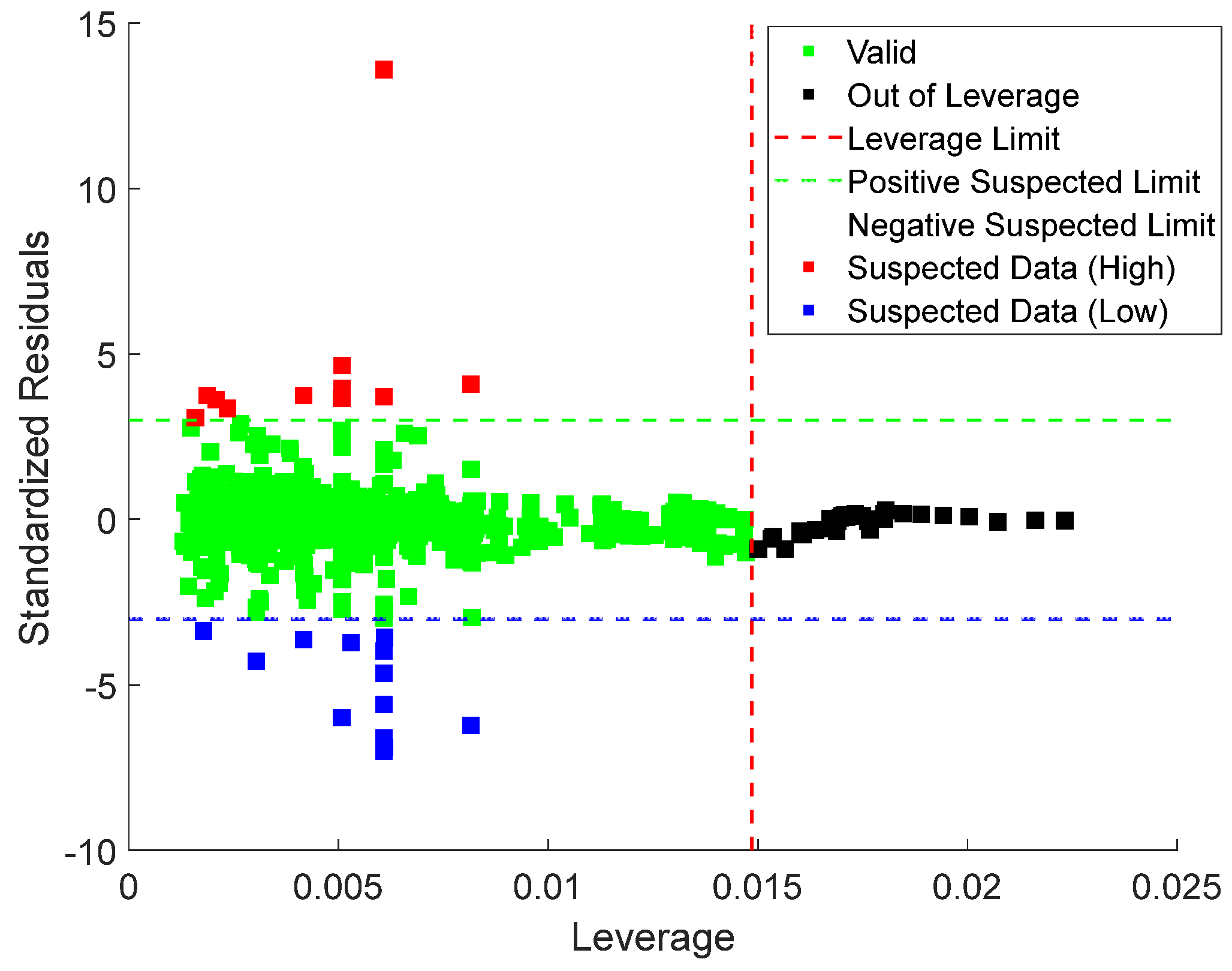
Lastly, leverage analysis was employed to systematically detect and evaluate outliers within the dataset. The implementation process involved the construction of a Williams plot. This diagnostic tool visually combines standardized residuals with the leverage values to visually identify influential points, outliers, and high-leverage observations of the model’s predictions, as shown in Equations (22) and (23), as follows:
Here, is the calculated leverage values and X is the matrix of predictor variables (with n samples and p predictors). The diagonal elements of the hat matrix denoted represent the leverage of the observation. High leverage values indicate that a data point has a significant influence on the fitted model. Also, represents the input parameter; is the number of data points; and denotes the transpose. , the standardized residual, is calculated based on the prediction error , root mean square error (RMSE), and leverage values . The Williams plot is presented in Figure 17, with the valid data points located within the region defined by the leverage threshold () and standardized residual boundaries. This region indicates the model’s applicability domain.
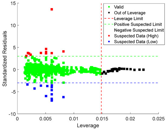
Figure 17.
William plots for stacking ensemble model proving the applicability of the model for predicting CO2 uptake in MOFs.
The leverage threshold is mathematically expressed in Equation (24), with a value of 0.015 for the current dataset. Data points with standardized residuals beyond or leverage values exceeding are identified as potential outliers. The region where is further divided into good high leverage (where ) and bad high leverage (where ) [41].
In this analysis, = 5 represents the number of input variables, while = 1212, indicating the total number of data points. The Williams plot was applied to the Stacking Ensemble model, as shown in Figure 15. The results show that 96.6% of the data points fall within the valid region, with leverage values between 0 and 0.015 (the upper limit ). Only 19 records exceeded the leverage threshold, while 22 exceeded the standardized residual limits, resulting in 41 out of 1212 records being flagged as potential outliers. Given that only a tiny fraction of data lies outside the valid region, the leverage analysis confirms the model’s applicability and the reliability of the experimental data.
5. Conclusions
This study developed a robust framework for predicting carbon dioxide (CO2) uptake in metal–organic frameworks (MOFs) using a suite of ensemble machine learning techniques. Five individual regression models; Random Forest, XGBoost, LightGBM, SVR, and MLP, were initially trained, capturing diverse patterns within the dataset. Subsequently, ensemble strategies including voting, weighted voting, stacking, and manual blending were evaluated to enhance prediction accuracy and generalizability. Among all the tested models, the stacking ensemble consistently outperformed the others, achieving the highest coefficient of determination (R2) and lowest error metrics. Diagnostic evaluations using cross plots, residual analyses, and prediction intervals confirmed the stacking model’s reliability across the full range of CO2-uptake values. Furthermore, permutation feature importance indicated that pressure (P) and temperature (T) were the most influential features driving adsorption behavior. The proposed ensemble learning approach demonstrated its capability to provide accurate and interpretable predictions without relying on expensive molecular simulations.
The dominance of Zn-centered samples in the current dataset may introduce bias and overfitting toward that class. To mitigate this, stratified sampling can ensure balanced representation of each metal center during train and validation splits, and synthetic oversampling methods such as SMOTE or ADASYN can augment underrepresented classes. A further option is to apply class-weighted loss functions or to use ensemble approaches with balanced bootstrap sampling in order to penalize misclassification of minority centers more heavily. Evaluation of overfitting should include per-class performance metrics such as balanced accuracy, macro F1 scores and confusion matrices to detect skewed errors. Finally, leave-one-metal-center-out cross-validation and learning-curve analyses would assess how well the model generalizes to novel metal-center chemistries.
6. Limitations and Recommendations
These findings suggest a strong potential for accelerating the screening of MOF candidates in carbon-capture workflows and facilitating rapid, data-driven decision-making in material-discovery pipelines. Although this study successfully predicted CO2 uptake in metal–organic frameworks (MOFs) using ensemble models, several limitations are acknowledged, and recommendations for future studies are proposed beloe.
- Primarily, the models were trained and validated solely on data from only five (5) metal centers. This approach does not fully capture the variety of base metals used in MOF design. Also, the input parameters included only physical conditions and textural properties. Future work can extend this framework by incorporating deep learning architectures and transfer-learning strategies. These models could potentially capture complex, non-linear interactions between the variables more effectively, leading to improved predictive accuracy for CO2 uptake in MOFs under diverse carbon-capture conditions.
- Another limitation is the selection of machine learning models. While base models have demonstrated strong predictive performance, they may not fully capture the non-linear interactions among pressure, temperature, SBET, VT, and CO2 adsorption. Hybrid descriptors that combine both experimental and structural data would improve model scalability and applicability across wider MOF classes and gas species. Incorporation of geometric-based and energy-based properties of MOFs to fully represent their structural and adsorption characteristics is recommended to improve the accuracy and generalizability of CO2-uptake-prediction models.
- In this study, we applied label encoding to the “metal center” feature for simplicity and computational efficiency. This choice may not fully capture the nuanced chemical effects of different metal sites. Future work should compare alternative schemes such as one-hot encoding, target (mean) encoding or learned embeddings to determine which best represents the metal’s influence on CO2 uptake.
Author Contributions
Conceptualization, P.L. and Z.I.; methodology, Z.I., P.L. and K.S.; software, Z.I., P.L. and N.J.O.; validation, P.L., K.S. and N.J.O.; formal analysis, Z.I.; investigation, Z.I.; data curation, E.T.B. and N.J.O.; writing—original draft preparation, Z.I. and P.L.; writing—review and editing, E.T.B., K.S. and N.J.O.; visualization, Z.I. and P.L.; supervision, E.T.B.; project administration, E.T.B. and P.L. All authors have read and agreed to the published version of the manuscript.
Funding
This research received no external funding.
Data Availability Statement
Data will be made available on request.
Conflicts of Interest
The authors confirm that they have no known conflicts of interest regarding the information provided in this study, nor have they received financial support for this work, which has influenced its content in any way.
Abbreviations
The following abbreviations are used in this manuscript:
| CO2 | Carbon dioxide |
| MOF | Metal–Organic Framework |
| SBET | BET surface area (m2/g) |
| SL | Langmuir surface area (m2/g) |
| VT | Pore volume (cm3/g) |
| P | Pressure (bar) |
| T | Temperature (K) |
| MC | Metal center |
| CO2 Uptake | Amount of carbon dioxide adsorbed (mmol/g) |
| RMSE | Root Mean Squared Error |
| R2 | Coefficient of Determination |
| MAE | Mean Absolute Error |
| SVR | Support Vector Regression |
| SR | Standard Residual |
| GNN | Graph Neural Network |
| MLP | Multi-Layer Perceptron |
| MLPNN | Multi-Layer Perceptron Neural Network |
| LSSVM | Least Squared Support Vector Machine |
| PSO | Particle Swamp Optimization |
| GO | Growth Optimization |
| CatBoost | Categorical Boosting |
| XGBoost | Gradient Boosting |
| XGB | Extreme Gradient Boosting |
| ET | Extra Trees |
| LightGBM | Light Gradient Boosting Machine |
| RF | Random Forest |
| PI | Prediction Interval |
| IQR | Interquartile Range |
| CI | Confidence Interval |
| EWE | Equal-weighted Ensemble |
| PWE | Performance-weighted Ensemble |
| Stack | Meta-model ensemble using predictions from multiple base learners |
| MB | Manual Blending |
| EWV | Equal Weighted Voting |
| WV | Weighted Voting |
References
- Li, X.; Zhang, X.; Zhang, J.; Gu, J.; Zhang, S.; Li, G.; Shao, J.; He, Y.; Yang, H.; Zhang, S.; et al. Applied machine learning to analyze and predict CO2 adsorption behavior of metal-organic frameworks. Carbon Capture Sci. Technol. 2023, 9, 100146. [Google Scholar]
- Longe, P.O.; Danso, D.K.; Gyamfi, G.; Tsau, J.S.; Alhajeri, M.M.; Rasoulzadeh, M.; Li, X.; Barati, R.G. Predicting CO2 and H2 Solubility in Pure Water and Various Aqueous Systems: Implication for CO2–EOR, Carbon Capture and Sequestration, Natural Hydrogen Production and Underground Hydrogen Storage. Energies 2024, 17, 5723. [Google Scholar]
- Prabowo, W.A.E.; Akrom, M.; Rustad, S.; Sutojo, T.; Dipojono, H.K.; Maezono, R.; Rusydi, F. Predicting CO2 adsorption in metal-organic frameworks: Integrating machine learning with virtual sample generation. Results Surf. Interfaces 2025, 19, 100505. [Google Scholar]
- Chao, C.; Deng, Y.; Dewil, R.; Baeyens, J.; Fan, X. Post-combustion carbon capture. Renew. Sustain. Energy Rev. 2021, 138, 110490. [Google Scholar]
- Achour, S.; Hosni, Z. ML-driven models for predicting CO2 uptake in metal–organic frameworks (MOFs). Can. J. Chem. Eng. 2025, 103, 2161–2173. [Google Scholar]
- Longe, P.O.; Davoodi, S.; Mehrad, M.; Wood, D.A. Robust machine-learning model for prediction of carbon dioxide adsorption on metal-organic frameworks. J. Alloys Compd. 2025, 1010, 177890. [Google Scholar]
- Amar, M.N.; Ouaer, H.; Ghriga, M.A. Robust smart schemes for modeling carbon dioxide uptake in metal− organic frameworks. Fuel 2022, 311, 122545. [Google Scholar]
- Moosavi, S.M.; Jablonka, K.M.; Smit, B. The role of machine learning in the understanding and design of materials. J. Am. Chem. Soc. 2020, 142, 20273–20287. [Google Scholar]
- Burner, J.; Schwiedrzik, L.; Krykunov, M.; Luo, J.; Boyd, P.G.; Woo, T.K. High-performing deep learning regression models for predicting low-pressure CO2 adsorption properties of metal–organic frameworks. J. Phys. Chem. C 2020, 124, 27996–28005. [Google Scholar]
- Longe, P.; Molomjav, S.; Tsau, J.-S.; Musgrove, S.; Villalobos, J.; D’ERasmo, J.; Alhajeri, M.M.; Barati, R. Techno-economic evaluation of CO2-EOR and carbon storage in a shallow incised fluvial reservoir using captured-CO2 from an ethanol plant. Geoenergy Sci. Eng. 2025, 246, 213559. [Google Scholar]
- Moosavi, S.M.; Nandy, A.; Jablonka, K.M.; Ongari, D.; Janet, J.P.; Boyd, P.G.; Lee, Y.; Smit, B.; Kulik, H.J. Understanding the diversity of the metal-organic framework ecosystem. Nat. Commun. 2020, 11, 4068. [Google Scholar] [CrossRef] [PubMed]
- Wang, J.; Liu, J.; Wang, H.; Zhou, M.; Ke, G.; Zhang, L.; Wu, J.; Gao, Z.; Lu, D. A comprehensive transformer-based approach for high-accuracy gas adsorption predictions in metal-organic frameworks. Nat. Commun. 2024, 15, 1904. [Google Scholar] [PubMed]
- Herm, Z.R.; Wiers, B.M.; Mason, J.A.; van Baten, J.M.; Hudson, M.R.; Zajdel, P.; Brown, C.M.; Masciocchi, N.; Krishna, R.; Long, J.R. Separation of hexane isomers in a metal-organic framework with triangular channels. Science 2013, 340, 960–964. [Google Scholar]
- Millward, A.R.; Yaghi, O.M. Metal−organic frameworks with exceptionally high capacity for storage of carbon dioxide at room temperature. J. Am. Chem. Soc. 2005, 127, 17998–17999. [Google Scholar] [PubMed]
- Wang, M.; Zeng, Q.; Chen, D.; Zhang, Y.; Liu, J.; Ma, C.; Jia, P. A machine learning feature descriptor approach: Revealing potential adsorption mechanisms for SF6 decomposition product gas-sensitive materials. J. Hazard. Mater. 2025, 481, 136567. [Google Scholar]
- Zhang, Z.; Cao, X.; Geng, C.; Sun, Y.; He, Y.; Qiao, Z.; Zhong, C. Machine learning aided high-throughput prediction of ionic liquid@ MOF composites for membrane-based CO2 capture. J. Membr. Sci. 2022, 650, 120399. [Google Scholar]
- Gulbalkan, H.C.; Aksu, G.O.; Ercakir, G.; Keskin, S. Accelerated Discovery of Metal–Organic Frameworks for CO2 Capture by Artificial Intelligence. Ind. Eng. Chem. Res. 2023, 63, 37–48. [Google Scholar]
- Park, H.; Yan, X.; Zhu, R.; Huerta, E.A.; Chaudhuri, S.; Cooper, D.; Foster, I.; Tajkhorshid, E. A generative artificial intelligence framework based on a molecular +diffusion model for the design of metal-organic frameworks for carbon capture. Commun. Chem. 2024, 7, 21. [Google Scholar]
- Choudhary, K.; Yildirim, T.; Siderius, D.W.; Kusne, A.G.; McDannald, A.; Ortiz-Montalvo, D.L. Graph neural network predictions of metal organic framework CO2 adsorption properties. Comput. Mater. Sci. 2022, 210, 111388. [Google Scholar]
- Abdi, J.; Hadavimoghaddam, F.; Hadipoor, M.; Hemmati-Sarapardeh, A. Modeling of CO2 adsorption capacity by porous metal organic frameworks using advanced decision tree-based models. Sci. Rep. 2021, 11, 24468. [Google Scholar]
- Lu, C.; Wan, X.; Ma, X.; Guan, X.; Zhu, A. Deep-Learning-Based End-to-End Predictions of CO2 Capture in Metal–Organic Frameworks. J. Chem. Inf. Model. 2022, 62, 3281–3290. [Google Scholar]
- Orhan, I.B.; Zhao, Y.; Babarao, R.; Thornton, A.W.; Le, T.C. Machine learning descriptors for CO2 capture materials. Molecules 2025, 30, 650. [Google Scholar] [CrossRef]
- Wan, H.; Fang, Y.; Hu, M.; Guo, S.; Sui, Z.; Huang, X.; Liu, Z.; Zhao, Y.; Liang, H.; Wu, Y.; et al. Interpretable Machine-Learning and Big Data Mining to Predict the CO2 Separation in Polymer-MOF Mixed Matrix Membranes. Adv. Sci. 2025, 12, 2405905. [Google Scholar]
- Breiman, L. Random forests. Mach. Learn. 2001, 45, 5–32. [Google Scholar]
- Chen, T.; Guestrin, C. Xgboost: A scalable tree boosting system. In Proceedings of the 22nd Acm Sigkdd International Conference on Knowledge Discovery and Data Mining, San Francisco, CA, USA, 13–17 August 2016; pp. 785–794. [Google Scholar]
- Ke, G.; Meng, Q.; Finley, T.; Wang, T.; Chen, W.; Ma, W.; Ye, Q.; Liu, T.-Y. Lightgbm: A highly efficient gradient boosting decision tree. 31st Conference on Neural Information Processing Systems. In Advances in Neural Information Processing Systems 30; Curran Associates, Inc.: Long Beach, CA, USA, 2017. [Google Scholar]
- Dietterich, T.G. Ensemble methods in machine learning. In International Workshop on Multiple Classifier Systems; Springer: Berlin/Heidelberg, Germany, 2000; pp. 1–15. [Google Scholar]
- Rokach, L. Ensemble-based classifiers. Artif. Intell. Rev. 2010, 33, 1–39. [Google Scholar]
- Zhou, Z.-H. Ensemble methods. Combining Pattern Classifiers; Wiley: Hoboken, NJ, USA, 2014; pp. 186–229. [Google Scholar]
- Warner, B.; Ratner, E.; Carlous-Khan, K.; Douglas, C.; Lendasse, A. Ensemble Learning with Highly Variable Class-Based Performance. Mach. Learn. Knowl. Extr. 2024, 6, 2149–2160. [Google Scholar]
- Aggarwal, S.; Gupta, S.; Gupta, D.; Gulzar, Y.; Juneja, S.; Alwan, A.A.; Nauman, A. An artificial intelligence-based stacked ensemble approach for prediction of protein subcellular localization in confocal microscopy images. Sustainability 2023, 15, 1695. [Google Scholar] [CrossRef]
- Kuncheva, L.I. Combining Pattern Classifiers: Methods and Algorithms; John Wiley & Sons: Hoboken, NJ, USA, 2014. [Google Scholar]
- Silva, P.; Vilela, S.M.; Tomé, J.P.; Paz, F.A.A. Multifunctional metal–organic frameworks: From academia to industrial applications. Chem. Soc. Rev. 2015, 44, 6774–6803. [Google Scholar]
- Naimi, A.I.; Balzer, L.B. Stacked generalization: An introduction to super learning. Eur. J. Epidemiol. 2018, 33, 459–464. [Google Scholar]
- Opitz, D.; Maclin, R. Popular ensemble methods: An empirical study. J. Artif. Intell. Res. 1999, 11, 169–198. [Google Scholar]
- Kalule, R.; Abderrahmane, H.A.; Alameri, W.; Sassi, M. Stacked ensemble machine learning for porosity and absolute permeability prediction of carbonate rock plugs. Sci. Rep. 2023, 13, 9855. [Google Scholar]
- Hoerl, A.E.; Kennard, R.W. Ridge regression: Biased estimation for nonorthogonal problems. Technometrics 1970, 12, 55–67. [Google Scholar]
- Guan, J.; Huang, T.; Liu, W.; Feng, F.; Japip, S.; Li, J.; Wu, J.; Wang, X.; Zhang, S. Design and prediction of metal organic framework-based mixed matrix membranes for CO2 capture via machine learning. Cell Rep. Phys. Sci. 2022, 3, 100864. [Google Scholar]
- Hyndman, R.J.; Athanasopoulos, G. Forecasting: Principles and Practice, 2nd ed.; OTexts.com/fpp2; OTexts: Melbourne, Australia, 2018. [Google Scholar]
- Biecek, P.; Burzykowski, T. Explanatory Model Analysis: Explore, Explain, and Examine Predictive Models; Chapman and Hall/CRC: Boca Raton, FL, USA, 2021. [Google Scholar]
- Williams, D. Generalized linear model diagnostics using the deviance and single case deletions. J. R. Stat. Soc. Ser. C (Appl. Stat.) 1987, 36, 181–191. [Google Scholar]

Disclaimer/Publisher’s Note: The statements, opinions and data contained in all publications are solely those of the individual author(s) and contributor(s) and not of MDPI and/or the editor(s). MDPI and/or the editor(s) disclaim responsibility for any injury to people or property resulting from any ideas, methods, instructions or products referred to in the content. |
© 2025 by the authors. Licensee MDPI, Basel, Switzerland. This article is an open access article distributed under the terms and conditions of the Creative Commons Attribution (CC BY) license (https://creativecommons.org/licenses/by/4.0/).