Instance Selection Strategies to Improve the Performance of Data-Driven Regression Models Applied to Industrial Systems

Abstract

The present study originally addresses the data reduction problem in industrial settings through the lens of instance selection procedures, aiming to enhance the quality of data-driven models by preserving only the most relevant characteristics from the available datasets. Unlike traditional approaches, the proposed Instance Selection Library (ISLib) is specifically designed to handle the unique challenges of industrial datasets, such as operational variability, sensor inaccuracies, and the need for interpretable results. ISLib introduces a novel methodology tailored for regression tasks, an underexplored area in instance selection research. Additionally, the paper explores the statistical characteristics of the reduced datasets, the impact of training data size and distribution, and the performance of models across various fault and anomaly types. ISLib was validated using three datasets, including the Tennessee Eastman Process and two real-world oil and gas applications. The findings emphasize, for the first time, the significance of employing a well-designed instance selection approach to achieve successful outcomes in practical industrial applications, particularly in regression machine learning problems. By bridging literature gaps and offering a user-friendly tool, this work advances data-driven process monitoring in industrial environments.

1. Introduction

The increasing demand for process safety, efficiency, and sustainability has led to the development of increasingly complex industrial plants [1]. This complexity is reflected in a higher degree of instrumentation and more intricate control and automation systems. For instance, in the oil and gas industry, a typical platform may rely on over 30,000 sensors continuously producing information [2], generating between 1 and 2 TB of data daily [3]. Leveraging this vast amount of data to improve operations is a significant challenge and one of the primary goals of process monitoring.

The significant and consistent advancements in computer hardware capacity observed in the last years [4] alongside the global trend interest in terms such as machine learning and artificial intelligence have created an unprecedented opportunity for process monitoring applications in real-world case scenarios [5]. Considering the context of Brazil’s oil and gas industry, for example, investments in R&D—which in 2022 summed up to approximately BRL 4.4 billion— have been experiencing a constant increase in the proportion of projects dedicated to digital solutions. According to data from the Brazilian National Agency of Petroleum, Natural Gas and Biofuels (ANP), this share exceeded 30% in 2023, compared to less than 2% in 2017 [6].

As much as those numbers might bring expectations regarding new developments and applications, some challenges must be addressed. For instance, a downside of these rapid and decentralized developments is that very few studies are devoted to the relevant issues that precede or follow the monitoring step, as pointed out by Ji and Sun (2022) [7] and Maharana et al. [8]. These questions, however, are essential for practical applications and are, in most cases, delegated to the scrutiny of the operation crew.

In particular, for real-world applications, data pre-treatment is of paramount importance due to the need to ensure the quality of the available data, which frequently contains noise, missing values, and outliers, as well as redundant, irrelevant, and meaningless pieces of information that can significantly impact the performance of data-driven models [9]. CrowdFlower (2016) [10] estimated that 60% of a data scientist’s time can be spent just on cleaning and organizing the data. A similar result was obtained by Anaconda Inc. (2020) [11], which showed that 45% of the time spent by data scientists was devoted to data cleansing and preparation. Considering that the number of digital solutions tends to increase, according to the amount of R&D in the subject, it becomes imperative, for industrial-scale applications, that steps such as the ones regarding data pre-treatment are adequately addressed and presented.

Data reduction is one of the most critical steps inside a data pre-treatment framework. In general, data reduction aims to optimize the overall dimension of the dataset while maintaining or improving its quality. This can be achieved by manipulating the number of columns (or features) and/or rows (or instances) of the datasets. The former is usually referred to as feature selection, and the latter is known as prototype or instance selection. In the field of process monitoring, the amount of published works dedicated to feature selection is overwhelmingly more significant than the number of papers on instance or prototype selection, accounting for approximately 98% of the articles available, according to Google Scholar [12]. This can be explained, among other things, by the fact that when dealing with tabular data, i.e., data organized in the form of observations as rows and attributes as columns, the impact of removing columns over rows on the size of the final dataset is more evident. In that way, if the goal is to reduce the dimension of the dataset, acting on the attributes instead of the observations seems more effective. Among the 2% dedicated to instance selection, most works published are concerned with classification problems [13], leaving a gap in the critical field of regression models.

The present work highlights the crucial role of a well-designed instance selection procedure in addressing regression problems within real industrial settings. It emphasizes how the thoughtful selection of representative subsets of operational data can address challenges such as sensor noise, missing values, and redundant observations that compromise model quality. The Instance Selection Library (ISLib) was developed and employed as a means to validate the relevance of instance selection and demonstrate its impact across diverse industrial datasets. ISLib provides a structured approach for data reduction through two sequential phases: unsupervised clustering to identify and rank operational regions and an incremental instance selection strategy to optimize the training dataset size. Unlike traditional approaches, ISLib is designed to handle the unique challenges of industrial datasets, such as operational variability, sensor inaccuracies, and the need for interpretable results.

To explore the implications of instance selection, ISLib was tested on three case studies: (i) a flare gas flowmeter anomaly detection framework, (ii) a soft sensor for oil fiscal meters, and (iii) the Tennessee Eastman Process (TEP) dataset. The results showcase how carefully selected instances improve model performance while reducing dataset size. By removing irrelevant data and enhancing representativeness, the study illustrates how instance selection can benefit fault detection, soft sensor development, and anomaly identification within industrial systems. Additionally, the paper explores the statistical characteristics of the reduced datasets, the impact of training data size and distribution, and the performance of models across various fault and anomaly types.

The remainder of the paper is organized as follows: Section 2 presents a background on instance selection applied to process monitoring; Section 3 details the methodology created for instance selection; Section 4 describes the obtained results when the proposed techniques are employed; and Section 5 summarizes the main conclusions and recommendations.

2. Background: Instance Selection in Industrial Process Monitoring

Traditional industrial process management relies on costly maintenance programs, leading to compromises in process availability. However, in today’s complex and competitive industrial landscape, efficient technologies are needed for asset management. Proactive maintenance schemes, such as conditional-based monitoring (CBM), enable informed decision-making by continuously monitoring process conditions. As a matter of fact, CBM has proven effective in extending equipment lifespan, reducing maintenance costs, and maximizing process availability [14].

Digital monitoring tools using data and machine learning techniques are gaining importance in modern industries [15,16]. These tools convert sensor data into statistical indicators, enabling the comprehensive assessment of process integrity. Indeed, adopting proactive maintenance strategies and leveraging digital monitoring tools based on data and machine learning techniques can be vital for effective industrial asset management. These approaches optimize equipment lifespan, minimize maintenance costs, detect faults, and enhance process availability, aligning with the demands of modern industrial operations [17].

Several works have been published in process monitoring using a data-driven approach to tackle real industrial cases. Lemos et al. (2021) [18] used an Echo State Network (ESN) in an oil and gas process plant to monitor the quality of critical flowmeters. Cortés-Ibáñez et al. (2020) [19] presented a pre-processing methodology for obtaining quality data in a crude oil refining process. In the framework proposed by the authors, data reduction was presented through the optics of outlier elimination and feature selection. Oliveira-Junior and de Arruda Pereira (2020) [20] developed a soft sensor for the Total Oil and Grease (TOG) value using data from an oil production platform. N. Clavijo et al. (2019) [21] used a data-driven approach to create a real-time monitoring application of gas metering in an oil onshore process plant. Zhang et al. (2019) [22] relied on PCA and clustering techniques to develop a sensor fault detection and diagnosis (FDD) for a water source heat pump air-conditioning system.

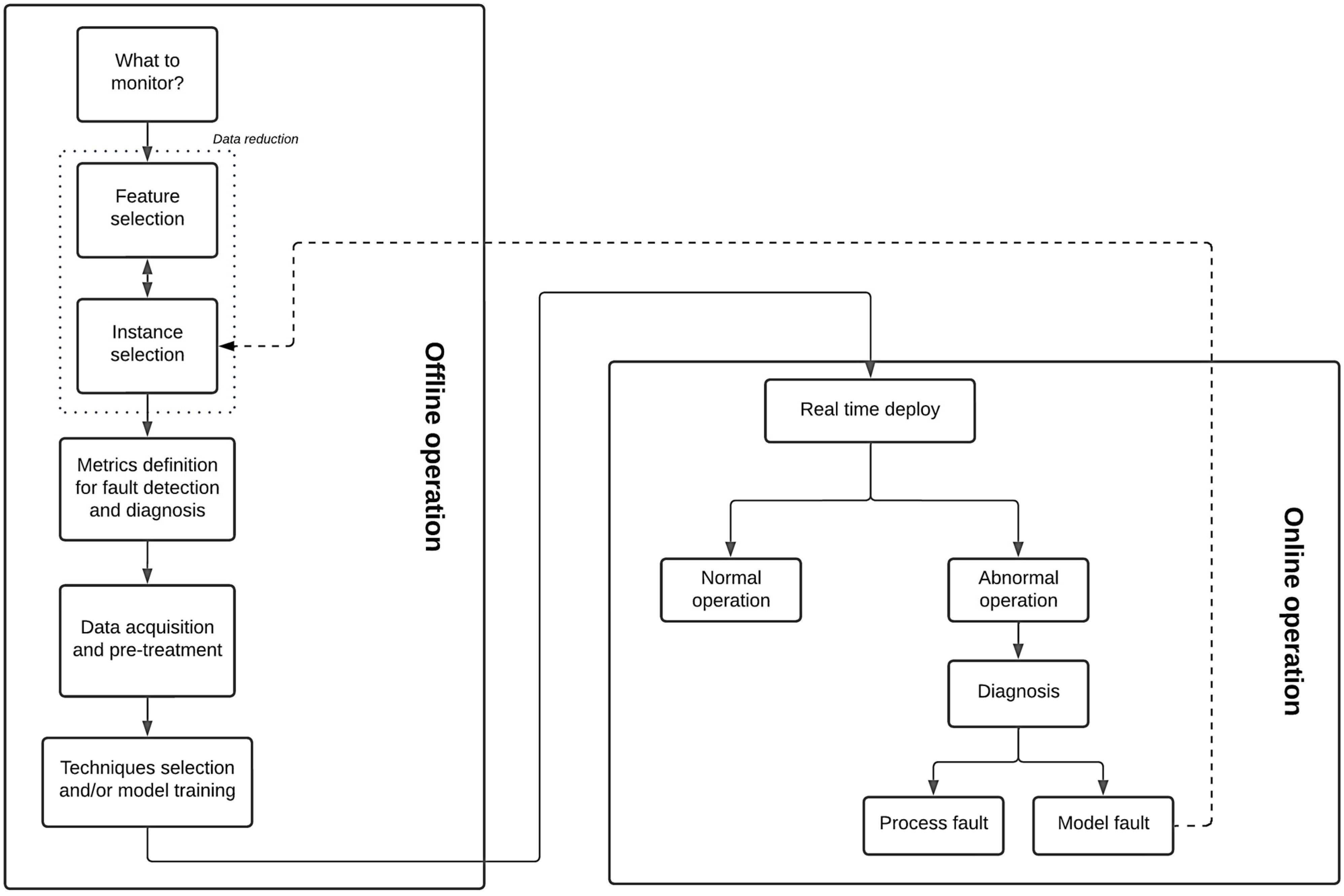
In any case, the deployment of a process monitoring task is, by definition, a multidisciplinary activity involving data scientists, base operators, process engineers, and an information technology team. This synergy can be crucial since numerous steps are required to implement a monitoring application successfully. Figure 1 proposes a general and detailed framework for a typical data-driven process monitoring deployment, encompassing each step, its key points, and boundaries for offline and online analyses. It is worth noting that the present work is focused on the data reduction problem and its importance for the general framework. If the reader should be interested in the other steps regarding a process monitoring deployment, comprehensive reviews can be found elsewhere [1,23,24,25,26,27,28].

As one can see in Figure 1, data reduction comprises one of the first steps in a process monitoring framework. Despite its importance, it is not uncommon for data scientists, or even companies that provide monitoring solutions, to delegate this step to base engineers or plant operators. This conviction arises from the fact that the operation team possesses a better knowledge of the process than any other group involved in the monitoring deployment task. Despite that, it should not be expected for operators or base engineers to perform a very deep analysis of the data. At best, they can bring and suggest an initial set of tags and instances to be further analyzed. Finding a representative period for training, however, might constitute a challenging task, presenting itself as one of the most important and time-consuming activities in building an industrial process monitoring model [7] since it necessarily requires going through and mining a large amount of data. In applications with hundreds of measurements, some information might be left out or, what is worse, from the model perspective, wrongly included in the final dataset.

Among the techniques to better condition the data, instance selection encompasses a variety of procedures and algorithms that are intended to select a representative subset from the initial training dataset [29]. According to Liu and Motoda (2002) [30], an instance selection procedure serves several main functions, such as enabling more computationally demanding models to handle larger datasets, focusing on the most relevant subsets of the data to potentially improve model performance, and cleaning the dataset by removing outliers or redundant instances that are considered irrelevant to understanding the data.

Historically, instance selection has been mostly used in classification problems, where the outputs are discrete and usually limited in possibilities [31]. For regression tasks, different approaches must be used since the output is continuous and, therefore, has an arbitrary number of possible values [29]. Besides that, there also seems to be a consensus that the predictor becomes better when the number of observations used to train the regression model increases, in such a way that reducing the dataset size would not make sense for regression. This last statement, however, can only be true if the data quality remains the same through all observations. In real-world scenarios, with processes subject to random variations and unexpected disturbances [7], transmitters prone to losing calibration, communication failures, poor control design, among other known limitations, this quality can hardly be guaranteed. Moreover, taking into consideration that most of the monitoring activity will be conducted by engineers and not data scientists, it becomes imperative, for the sake of the success of any industrial deployment, that instance selection procedures are not only executed but also presented in the best way possible for the final users to interpret them and take actions.

By doing so, the original size of the dataset can be reduced and the predictive capability of the resulting models may even improve [32]. In other words, after instance selection is applied on a tabular dataset ${\mathit{X}}^{N\times M}$ with $N$ observations and $M$ measurements, it is expected that $P\left(h\left({\mathit{X}}^{N\times M}\right)\right) \cong P\left(h\left({\mathit{X}}^{S\times M}\right)\right)$, where $P$ is a performance measure for the learning algorithm $h$, and ${\mathit{X}}^{S\times M}$ is a subset of ${\mathit{X}}^{N\times M}$ with $S<N$. In supervised learning, ${\mathit{X}}^{N\times M}$ can be represented by a distinct set of inputs and outputs $\left\{{\mathit{X}}^{N\times M},{\mathit{Y}}^{N\times p}\right\}$, with $\mathit{Y}$ representing the output (or predicted) matrix, and $\mathit{Y}\in {\mathbb{R}}^{\mathit{p}}$.

As an approach to apply instance selection to regression problems, Guillen et al. (2010) [33] used the concept of mutual information, normally applied in the field of feature selection, to select the best input vectors to be used during the model training. Stojanović et al. (2014) [34] also used mutual information to select training instances for long-term time series prediction. By selecting instances that shared a large amount of mutual information with the current forecasting instance, the authors could reduce the error propagation and accumulation in their case studies. Arnaiz-González et al. (2016) [32] adapted the well-known DROP (Decremental Reduction Optimization Procedure) family of instance selection methods for classification to regression. In a different approach, Arnaiz-González et al. (2016) [29] applied the popular classification noise filter algorithm ENN (Edited Nearest Neighbor) to regression problems. To achieve this, the authors discretized the output variable, framing the problem as a classification task. Song et al. (2017) [35] proposed a new method, called DISKR, based on the KNN (K-Nearest Neighbor) Regressor, which removes outlier instances and then creates a ranking sorted by the contribution to the regressor. DISKR was applied to 19 cases and showed similar prediction ability compared to the full-size dataset model. More recently, Kordos et al. (2022) [13] developed an instance selection procedure based on three serial steps. The first step decomposes the data using fuzzy clustering; the second uses a genetic algorithm to perform instance selection for each cluster separately; and the combined results are weighted to provide a single output. The method was applied to several open benchmarks and generally improved the predictive model performance while reducing its size. Li and Mao (2023) [36] presented a novel noise-filtering technique specifically designed for regression problems with real-valued label noise. The proposed method introduces an adaptive threshold-based noise determination criterion and a noise score to effectively identify and eliminate noisy samples while preserving clean ones. Its performance was evaluated across various controlled scenarios, including synthetic datasets and public regression benchmarks, demonstrating superiority over state-of-the-art methods.

It is worth noting that the studies mentioned above used well-known open datasets from various sources and fields. From the process monitoring perspective and all the challenges it poses for data pre-processing, a relevant literature gap still exists when applying such methods to real industrial data. One of the key contributions of this work is addressing the gap in instance selection for regression problems by leveraging real datasets extracted from various Petrobras units. The proposed methodology is specifically tailored for practical industrial applications, ensuring that data utilization and result presentation are directly aligned with the operational requirements of end-users.

3. Instance Selection Library (ISLib)

In the present study, a novel Python library named Instance Selection Library (ISLib) was developed to identify the most important operating regions of a dataset focusing on regression problems.

According to the taxonomy presented by García et al. (2012) [37], ISLib performs its search in two steps, as described below.

3.1. Batch Instance Selection Using Ranked Clusters

Ranked clusters are groups of operational data that are organized based on their similarities and are prioritized according to how much they improve model accuracy. This approach helps in identifying the most important operational areas while reducing irrelevant data. By using error metrics like Mean Squared Error (MSE) to assign rankings, these clusters highlight the parts that are more crucial for making predictions.

In the initial step, an unsupervised clustering algorithm is applied to find similar subgroups within the initial data. The goal at this stage is to identify potential operational regions that should be included in the final dataset. Among the various techniques available, partitioning methods are known for their efficiency in terms of computational complexity and memory requirements [13]. The ISLib library uses the K-Means clustering algorithm [38] due to its simplicity and fast convergence. The optimal number of clusters is determined using the elbow method, balancing intra-cluster variance and computational efficiency. In other words, to overcome the drawback of having to define the number of clusters beforehand, in the present application, K was defined according to an objective function that minimizes the clustering loss function while trying to keep the value of clusters at its minimum.

The clusters obtained from K-Means are then ranked by their Mean Squared Error (MSE) when trying to predict the other regions. This is achieved by training a model ($h$) with all the observations contained in region $i$, with $i \in \left(1, \dots , K\right)$, and tested against all clusters $j$, with $j \in \left(1, \dots , K\right)$ and $j \ne i$. Figure 2 depicts an example of the results obtained from this analysis, showing the clusters ranked and one of the $M$ measurements that compose the dataset to illustrate some key points. As one can see in Figure 2, the model trained only with data from Cluster 1 results in a better performance $P$, with $P$ in this case being the MSE value when trying to predict data from Clusters 2 and 3. On the other hand, a model trained using only data from Cluster 3 seems to perform worse when presented with data from Clusters 1 and 2. The model $h$ used in ISLib assumes the form of a Principal Component Analysis (PCA), if the objective is to provide data for an unsupervised model, or a Regression Tree (RT), if the goal is a supervised model. Principal Component Analysis (PCA) and Regression Tree (RT) were chosen due to their robustness and low computational complexity, which align well with industrial datasets characterized by large volumes and high variability. While other lightweight models such as Support Vector Machines (SVM) could be used, PCA has been widely applied in the field of process monitoring [23,39,40] due to its ability to effectively reduce data dimensionality while preserving essential variability, and RT simplifies regression tasks in scenarios where interpretability and speed are important [41].

The pseudocode that performs the previously described steps is displayed in Algorithm 1.

Algorithm 1 Pseudocode for ranking most important clusters in ISLib
Require: Initial dataset $X$, configuration parameters $\mathrm{C}$
1:	for $K\leftarrow to{C}_{\mathit{max}\_\mathit{clusters}}$ do
2:	Define objective function $F\left(K\right)=\mathrm{Loss}\left(KMeans\right)+\mathsf{\lambda }K$ where $\mathsf{\lambda }$ is a regularization parameter
3:	Perform K-Means clustering on $X$
4:	if $F\left(K\right)>F\left(K-1\right)$ then
5:	$K_{\mathit{final}}\leftarrow K-1$
6:	Break
7:	for $i\leftarrow to{K}_{\mathit{final}}$ do
8:	if problem is supervised then
9:	$h \leftarrow$ Regression Tree ($C_{RT}$)
10:	Train $h$ on $\left(X_i,Y_i\right)$
11:	Test $h$ on $\left(X_j\right)$ where $j \ne i$
12:	${\mathit{MSE}}_i\leftarrow {\displaystyle \frac{1}{N_j}}{\sum }_{j=1}^{N_j}{\left(Y_j-\widehat{Y_j}\right)}^2$ where $N_j$ is the number of observations in $j$
13:	else if problem is unsupervised then
14:	$h \leftarrow$ PCA ($C_{CPV}$)
15:	Train $h$ on $X_i$
16:	Test $h$ on $X_j$ where $j \ne i$
17:	${\mathit{MSE}}_i\leftarrow {\displaystyle \frac{1}{N_j}}{\sum }_{j=1}^{N_j}{\left(X_j-\widehat{X_j}\right)}^2$ where $N_j$ is the number of observations in $j$
	return Ordered $K_{\mathit{final}}$ clusters by MSE values

In Algorithm 1, the hat sign (^) denotes that the input vector ($\mathit{X}$) or the target vector ($\mathit{Y}$) is generated by the model $h$. In a supervised model, MSE is calculated based on the predicted values of $\mathit{Y}$, given $\mathit{X}$, using an RT with hyperparameters $C_{RT}$. On the other hand, in an unsupervised model, the MSE is calculated using the reconstructed values of $\mathit{X}$ obtained from PCA. The Cumulative Percentage Variance ($C_{CPV}$) criterion [42] is used to determine which components are retained as the most important ones.

The ranked clusters, along with the visual representation of the operational regions, assist in selecting the most desirable subsets to keep. Although ISLib automates the analysis, it is essential to ratify the conclusions with system knowledge. In other words, the final decisions still require human validation and evaluation.

3.2. Incremental Instance Selection Using a Crescent Window Strategy

Based on the subsets provided by the previous step, the goal in this second part is to define the minimum size of the training window from which the inclusion of additional points would not enhance the predictive power of the trained model. For this, several models are generated by increasing the training window size $S$, with $0<S<N$, to absorb, with each new model, more information from the dataset. During this process, the testing period does not remain fixed, and it is considered the fraction of the training window not used by the training itself. Thus, with each new model, the data used for training have their size increased by a window, while the data for testing are decreased by the same amount. Figure 3 illustrates the adopted procedure, while Algorithm 2 shows its pseudocode. The employed terminology follows the same convention as presented in Algorithm 1. The overlapping time series on the $M$ axis indicate different features along $N$ samples in the same training/test split configuration. The figure depicts this ratio changing along the $S$ axis, maintaining the total size (training + test) constant.

Algorithm 2 Pseudocode for finding the minimum window size in ISLib
Require: Dataset $X$, configuration parameters $C$
1:	for $S\leftarrow C_{min\_size\_window}$  to $N$ , where $N$  is the number of rows of the dataset, do
2:	if problem is supervised then
3:	$h \leftarrow$  Regression Tree ($C_{RT}$ )
4:	Train $h$ on $\left(X\left[0:S\right],Y\left[0:S\right]\right)$
5:	Test $h$ on $\left(X\left[S+1:N\right]\right)$
6:	$MS{E}_S\leftarrow {\displaystyle \frac{1}{N-S}}\sum {\left(Y\left[S+1:N\right]-\widehat{Y}\left[S+1:N\right]\right)}^2$
7:	else if problem is unsupervised then
8:	$h \leftarrow$  PCA($C_{CPV}$ )
9:	Train $h$  on $\left(X\left[0:S\right]\right)$
10:	Test $h$  on $\left(X\left[S+1:N\right]\right)$
11:	$MS{E}_S\leftarrow {\displaystyle \frac{1}{N-S}}\sum {\left(X\left[S+1:N\right]-\widehat{X}\left[S+1:N\right]\right)}^2$
12:	store $MS{E}_S$
13:	$min\_MSE\leftarrow \mathit{min}\left(MS{E}_S\right)$
14:	$min\_size\_window \leftarrow$  index of $min\_MSE$
	return $min\_size\_window$

Once the dataset is submitted to the steps presented in Algorithm 2, two possible scenarios can arise. Firstly, if the model $h$ displays strong generalization capabilities, the MSE profile is expected to exhibit a decaying pattern as the training window expands, indicating improvement in model performance. Conversely, if the dataset presents regions too distinct to allow the model to generalize the process behavior well, the MSE profile is likely to reflect these regions. In such cases, the trend may show sudden decreases as the model learns each new state.

It is worth noting that even though the two steps were designed to be executed sequentially, it is possible to perform them either sequentially or independently, depending on the objectives and the initial data quality. For example, clustering could be omitted for datasets with pre-defined operational regions, focusing instead on incremental instance selection to determine optimal training windows. A flowchart outlining these decisions is presented in Figure 4.

The ISLib library was integrated into the standard process monitoring tool from Petrobras, called SmartMonitor [5], and has been used to provide users with quick insights about their datasets, speeding the pre-processing steps and obtaining optimized regression models tailored to their specific applications. This structured and user-centric approach ensures that ISLib not only addresses theoretical gaps in instance selection for regression tasks but also meets the operational demands of industrial applications. The next section showcases some of the results obtained by ISLib.

4. Results and Discussion

4.1. Methodology

Results from ISLib are presented here for three different cases: (I) the Tennessee Eastman Process (TEP) dataset, (II) an offshore flare gas flowmeter fault detection framework, and (III) an offshore oil fiscal meter soft sensor. The datasets used in this study differ in several aspects, including sensor types, environmental conditions, and operational modes. For instance, the flare gas flowmeter dataset involves high flow velocities and varying gas compositions, while the oil flowmeter dataset is influenced by temperature and pressure variations. These differences highlight the adaptability of the proposed methodology to diverse industrial scenarios.

Table 1. Summary of evaluated cases.

Dataset	Objective	Model (h)	Dataset Initial Size (N)
TEP	Unsupervised model	Principal Component Analysis (PCA)	500
Flare gas flowmeter	Unsupervised model	Autoencoder (AE)	30,775
Oil flowmeter	Supervised model	Echo State Network (ESN)	53,309

presents the cases evaluated and some of their characteristics.

The performances of the models were measured by the operator $P$, which was calculated in two ways: before the final model training—or, in other words, during ISLib processing—the error through the observations was estimated by the MSE value according to Algorithms 1 and 2; after the final models listed in Table 1 were obtained, their performances were then compared by the Squared Prediction Error (SPE), defined as $\mathrm{S}\mathrm{P}\mathrm{E}:=\sum _{i=1}^K{\left({\mathit{Z}}_i-{\widehat{\mathit{Z}}}_i\right)}^2$, where $\mathit{Z}=\mathit{X}$ and $K=M$ for unsupervised models or $\mathit{Z}=\mathit{Y}$ and $K=p$ for supervised models. Again, the superscript ^ indicates the predicted values from the model. The decision to use two distinct metrics—MSE and SPE—reflects their widespread application in different phases of model evaluation. MSE is commonly used during training and validation to measure overall predictive accuracy across datasets. On the other hand, SPE is a well-established metric for anomaly detection [43], as it focuses on identifying deviations in individual observations based on reconstruction error.

Two outputs were generated for each tested case: one model using the instances selected by ISLib and another using the full-size dataset. An abnormal event is detected if the SPE value exceeds a predefined threshold (SPE_lim). If the residues follow a Gaussian distribution, the control limit can be characterized by a chi-squared test [31]. A more general approach might use a percentile value from the training or validation period as a threshold (typically between 95% and 99%) [21]. The SPE_lim value is then kept constant and serves as a boundary for the normal operation condition or for an alarm detection heuristic.

As indicated in Table 1, this study presents results from various algorithms in addition to the models used within ISLib for analysis (PCA or RT). Since the main goal of this research is to address the importance and impact of pre-processing steps such as data reduction, detailed information regarding these models will not be extensively covered, given the relatively large number of surveys published in the open literature in this area. The interested reader might refer to Melo et al. (2024) [23] and Aldrich and Auret (2013) [31] for the employed PCA methodology; to Hallgrímsson et al. (2020) [44] and Zhu et al. (2022) [45] for the Autoencoder (AE) model detail; and to Lemos et al. (2021) [18] for the Echo State Network (ESN) application.

Finally, due to confidentiality reasons, all results from the second and third cases from Table 1 will be shown with normalized scales. Also, all units and stream names will be anonymized for the same reason.

4.2. Tennessee Eastman Process (TEP)

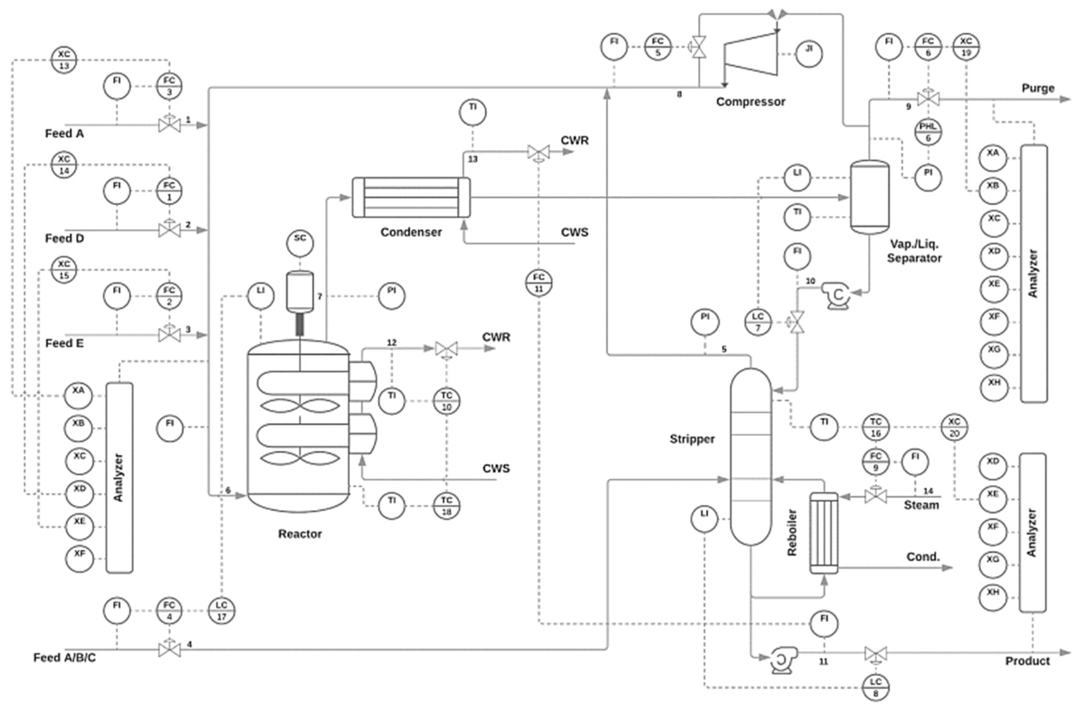
The first study used the well-known TEP dataset proposed by Eastman Chemical Company for evaluating process control and monitoring techniques [24,46]. The system comprises five major units: (I) a reactor, (II) a condenser, (III) a gas compressor, (IV) a separator vessel; and (V) a stripper. The main goal of this system, as indicated by the following reactions, is to produce the desired liquid (liq) products G and H from the gaseous (g) reactants A, C, D, and E.

A(g) + C(g) + D(g) → G(liq), Product 1

A(g) + C(g) + E(g) → H(liq), Product 2

A(g) + E(g) → F(liq), Byproduct

3D(g) → 2F(liq), Byproduct

The remaining unit operations in the process aim to purify the products from the reaction, separating them from the generated byproducts and inert products present in the system. The process has 11 manipulated variables and 41 measurements. Figure 5 shows the process flowchart with all variables and control loops.

The used datasets are available in Rieth et al. (2017) [47] and can be divided into two groups: a normal operating period for model training and a second group containing 21 different failure modes. Table 2,

Table 3. Process measurements in the TEP process.

Nº	Description	Nº	Description
1	A Feed (stream 1)	22	Separator Cooling Water Outlet Temp
2	D Feed (stream 2)	23	Component A
3	E Feed (stream 3)	24	Component B
4	A and C Feed (stream 4)	25	Component C
5	Recycle Flow (stream 8)	26	Component D
6	Reactor Feed Rate (stream 6)	27	Component E
7	Reactor Pressure	28	Component F
8	Reactor Level	29	Component A
9	Reactor Temperature	30	Component B
10	Purge Rate (stream 9)	31	Component C
11	Product Sep Temp	32	Component D
12	Product Sep Level	33	Component E
13	Prod Sep Pressure	34	Component F
14	Prod Sep Underflow (stream 10)	35	Component G
15	Stripper Level	36	Component H
16	Stripper Pressure	37	Component D
17	Stripper Underflow (stream 11)	38	Component E
18	Stripper Temperature	39	Component F
19	Stripper Steam Flow	40	Component G
20	Compressor Work	41	Component H
21	Reactor Cooling Water Outlet Temp

, and

Table 4. Fault description of TEP.

Fault Number	Description	Type
IDV (1)	A/C feed ratio, B composition constant (stream 4)	Step
IDV (2)	B composition, A/C ratio constant (stream 4)	Step
IDV (3)	D feed temperature (stream 2)	Step
IDV (4)	Reactor cooling water inlet temperature	Step
IDV (5)	Condenser cooling water inlet temperature	Step
IDV (6)	A feed loss (stream 1)	Step
IDV (7)	C header pressure loss-reduced availability (stream 4)	Step
IDV (8)	A,B,C feed composition (stream 4)	Random variation
IDV (9)	D feed temperature (stream 2)	Random variation
IDV (10)	C feed temperature (stream 4)	Random variation
IDV (11)	Reactor cooling water inlet temperature	Random variation
IDV (12)	Condenser cooling water inlet temperature	Random variation
IDV (13)	Reaction kinetics	Slow drift
IDV (14)	Reactor cooling water	Valve sticking
IDV (15)	Condenser cooling water	Valve sticking
IDV (16)–(20)	Unknown	Unknown
IDV (21)	Valve (stream 4)	Constant position

show, respectively, the manipulated variables, available measurements, and failure events with their descriptions.

Table 2. Manipulated variables in the TEP process.

Nº	Description	Nº	Description
1	D Feed Flow (Stream 2)	7	Separator Pot Liquid Flow (stream 10)
2	E Feed Flow (stream 3)	8	Stripper Liquid Product Flow (stream 11)
3	A Feed Flow (stream 1)	9	Stripper Steam Valve
4	A and C Feed Flow (stream 4)	10	Reactor Cooling Water Flow
5	Compressor Recycle Valve	11	Condenser Cooling Water Flow
6	Purge Valve (stream 9)

Table 2. Manipulated variables in the TEP process.

Nº	Description	Nº	Description
1	D Feed Flow (Stream 2)	7	Separator Pot Liquid Flow (stream 10)
2	E Feed Flow (stream 3)	8	Stripper Liquid Product Flow (stream 11)
3	A Feed Flow (stream 1)	9	Stripper Steam Valve
4	A and C Feed Flow (stream 4)	10	Reactor Cooling Water Flow
5	Compressor Recycle Valve	11	Condenser Cooling Water Flow
6	Purge Valve (stream 9)

Figure 5. Process flowsheet of the Tennessee Eastman Process (TEP), depicting five main operational units: reactor, condenser, compressor, separator, and stripper [48].

Figure 5. Process flowsheet of the Tennessee Eastman Process (TEP), depicting five main operational units: reactor, condenser, compressor, separator, and stripper [48].

As described in the methodology, the normal operation data from TEP were presented to ISLib to create an alternative reduced dataset. Since the data presented by Rieth et al. (2017) simulated just one operating point [47], with all the events listed in Table 4 being deviations from this steady-state condition, the first step from ISLib was bypassed, as indicated by Figure 4, and the entire initial set of 500 observations was directly provided to the enlarging window strategy stage. The results from the reduced dataset model were then compared to those obtained from the full dataset model. Given that the ultimate objective was to create a PCA model for fault detection, the ISLib analysis followed the unsupervised approach outlined in Algorithm 2.

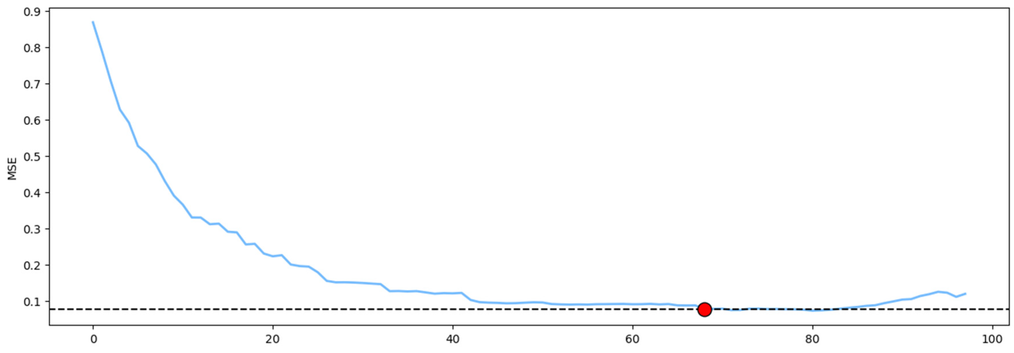
Figure 6 illustrates the MSE values obtained by each PCA model as the training dataset size increases incrementally. Since the initial dataset corresponds to a clearly defined operating region, the MSE profile exhibits a consistent decreasing trend as the model retains more information from the provided data. The dashed line in Figure 6 represents the minimum MSE value obtained, accounting for a 10% tolerance. The red dot indicates the point at which the MSE reaches this minimum. In the context of the present study, this value—equivalent to 340—represents a dataset reduction of 32%, when compared to the original data size of 500 observations.

The obtained results generated two subsequent PCA models: one referred to as “reduced dataset,” which used only the first 340 measurements from the original training dataset, and the other as “full dataset model,” incorporating the entire data. Both models used a C_CPV of 90% and were tested with different events from Table 4. For this analysis, only cases with documented good PCA performance were included. 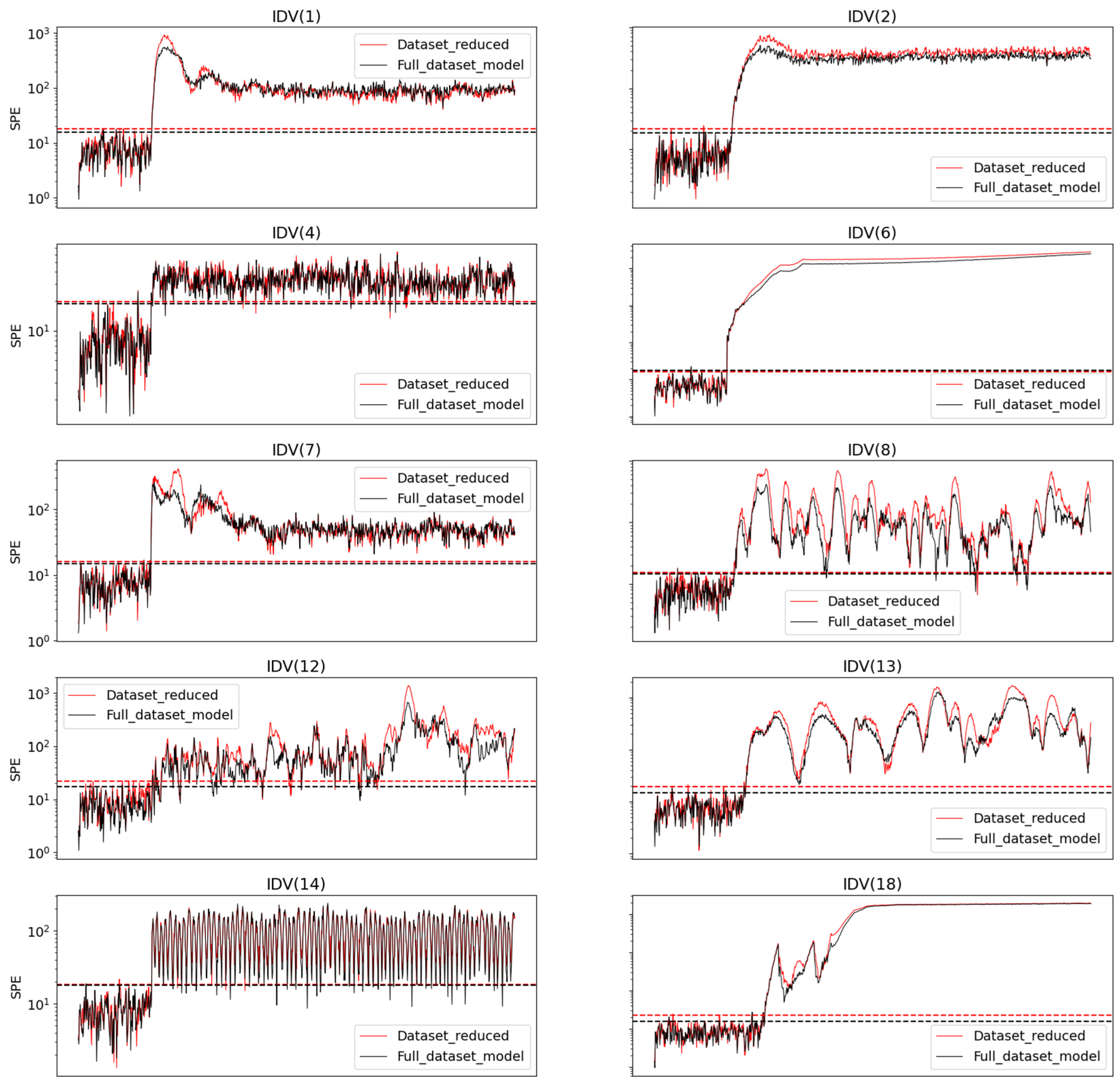Figure 7 shows the SPE profiles obtained for the two models. The dashed lines, calculated as the 99th percentile of the respective training SPE, serve as the basis for anomaly detection. As one can see, the behavior of the reduced model was similar to that of the complete model, with both detecting the anomalies almost simultaneously. In some cases, such as in IDV (2) and IDV (6), the reduced model was even more forceful in pointing out the anomaly, evidenced by the larger difference between the SPE values during normal and faulty periods. The dataset optimized by the methodology resulted in a decrease of approximately 10% in the model’s training time. Nonetheless, in practical terms, for this case the response to the anomaly is quite evident in both monitoring strategies.

Table 5. Results for anomaly detection using full and reduced datasets for training.

	MSE Before Anomaly		FN After Anomaly
Fault Index	Full Dataset	Reduced Dataset	Full Dataset	Reduced Dataset
1	6.8	6.7	2	2
2	7.9	7.8	11	11
4	9.1	8.7	9	21
6	8.7	8.6	0	0
7	7.6	8.5	0	0
8	8.6	8.1	31	18
12	8.4	9.2	31	44
13	7.0	7.7	39	39
14	8.1	8.7	36	7
18	8.7	8.2	78	80
Average	8.1	8.2	24	22

presents similar results, but in a quantitative format. The fault indices evaluated from Table 4 are listed in the first column. The second and third columns compare the MSE values obtained with the full dataset PCA against the reduced dataset model. Both performances were computed using the initial portion of the test dataset, where the anomaly had not yet occurred, as outlined by the low SPE values in Figure 7. Columns four and five correspond to the period during the presence of the fault. In this scenario, by knowing exactly where the anomaly begins, it is possible to calculate the number of false negative (FN) points obtained for each model; or, in other words, how many observations rely below the respective 99th percentile line after the fault initiation.

Averaging all cases, it is possible to notice the similar performance of both models in the test dataset. This is a notably interesting result because it demonstrates that even for a simulated scenario, confined to a single operational region, with known and constant uncertainties throughout the samples, it was possible to significantly reduce the dataset dimension without compromising the quality of the final model. As illustrated in the upcoming examples, in real-world scenarios where operational regions are not well-defined, making it challenging to identify a representative training dataset, the importance of employing instance selection techniques becomes even more pronounced.

4.3. Flare Gas Flowmeter

In offshore oil facilities, flaring gas is the action of burning waste crude natural gas that is not possible to process or sell [49]. Because of its impact on carbon emissions, in Brazil, ANP limits the authorized burning and losses, establishing parameters for its control [50].

Measuring the amount of gas sent to flare, however, does not constitute a simple task since it involves dealing with large pipe diameters, high flow velocities over wide measuring ranges, gas composition changes, condensate, etc. [51]. Despite that, it is common to install flared gas metering only on the main flare header [52], making its reliability crucial for ensuring a safe operation.

In this application, a monitoring system using AE was specifically designed to detect anomalies in the flare gas meter of a Petrobras oil production platform. The flare gas flowmeter dataset was obtained from the historical operational data of a Petrobras oil production platform and comprised 30,775 observations and five features, including one volume flow measurement, one pressure transmitter, one level signal and two temperatures. Due to confidentiality, the dataset is not publicly available but can be shared upon request under specific agreements. 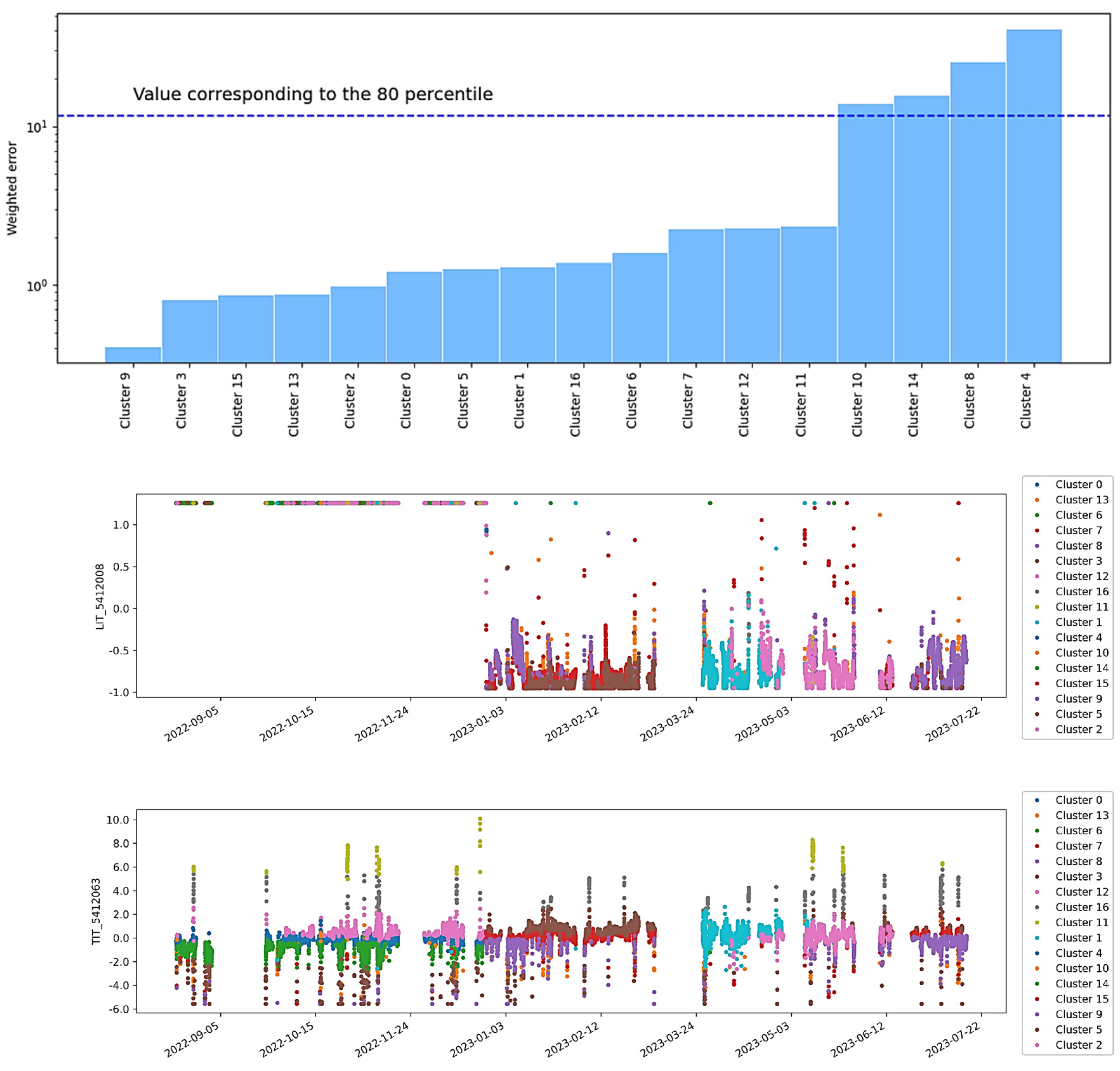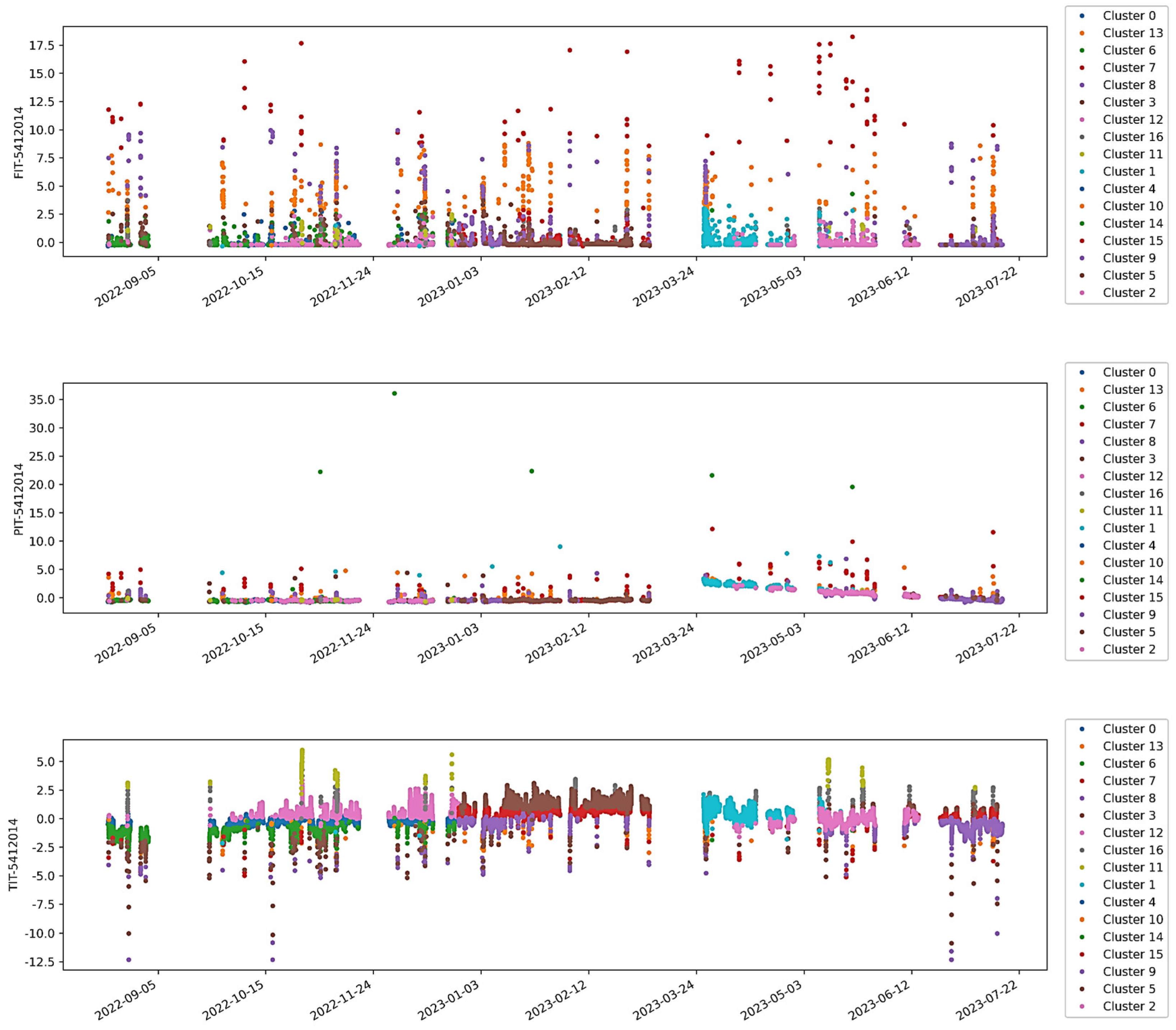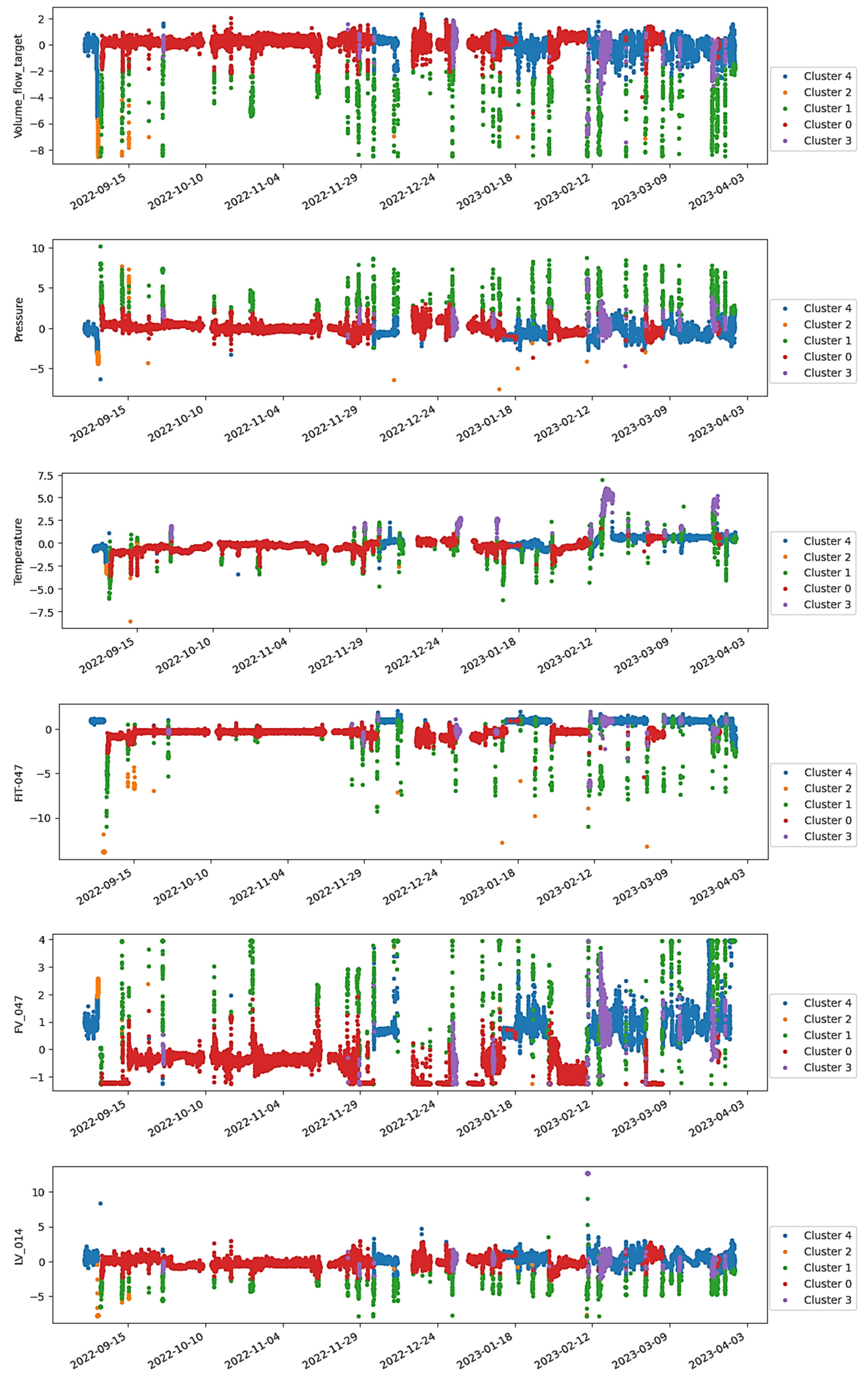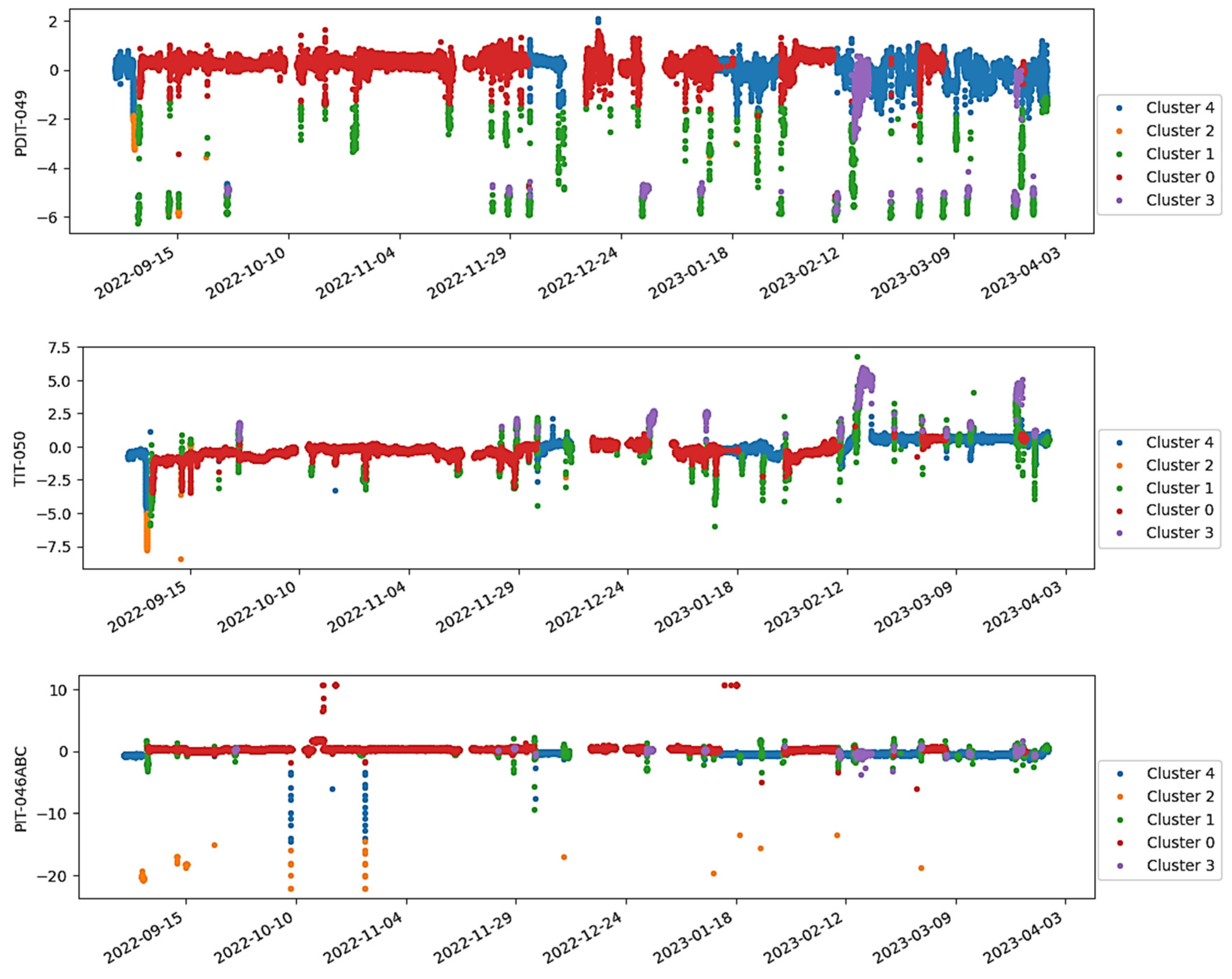Figure 8 shows the results obtained for the batch instance selection stage from ISLib. The colors from the trends highlight the clusters derived from the K-Means analysis, and the bar chart shows the MSE for each cluster, when trying to predict all other operational regions.

Based on the previous results, the monitoring team responsible for the system decided to exclude the regions associated with the highest MSE values, notably clusters 4, 10, and 14, from subsequent analyses. This decision was made on the assumption that these regions were linked to production interruptions, outliers, or other non-representative operation modes.

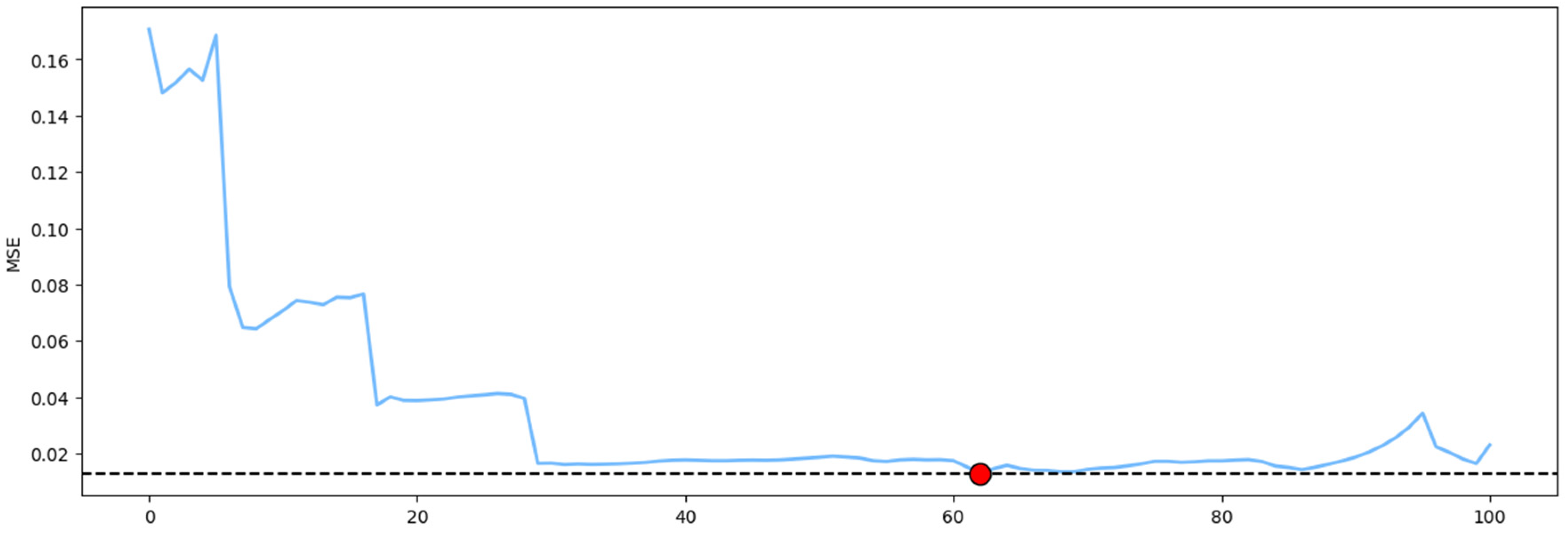
Figure 9 shows the enlarging window approach from ISLib using the regions defined by the remaining clusters.

The trend observed in Figure 9 shows one of the most important results expected from this analysis. As one can see, the error profile has two significant discontinuities as the training window increases. Those steps mark the points in the dataset where major changes happen. In other words, if the dataset contains different operational regions—as deliberated through the clustering analysis—as the training window increases, the testing window consequently decreases, becoming more concentrated in regions that might not have been presented to the model yet. Because of this poor generalization capacity from the model, the MSE tends to increase at first. As soon as a new condition, never experienced by the model, is incorporated into the training data, the resulting model can identify this new condition, yielding the steep drop observed in the MSE trend. The cycle restarts if new conditions are present in the remaining part of the dataset. If, however, the last unexplored subset is presented to the model, the MSE profile may show no more considerable variations. At this stage, as already mentioned, including new instances for training would not increase the predictive power of the regression model, meaning that the minimum window size had been achieved. 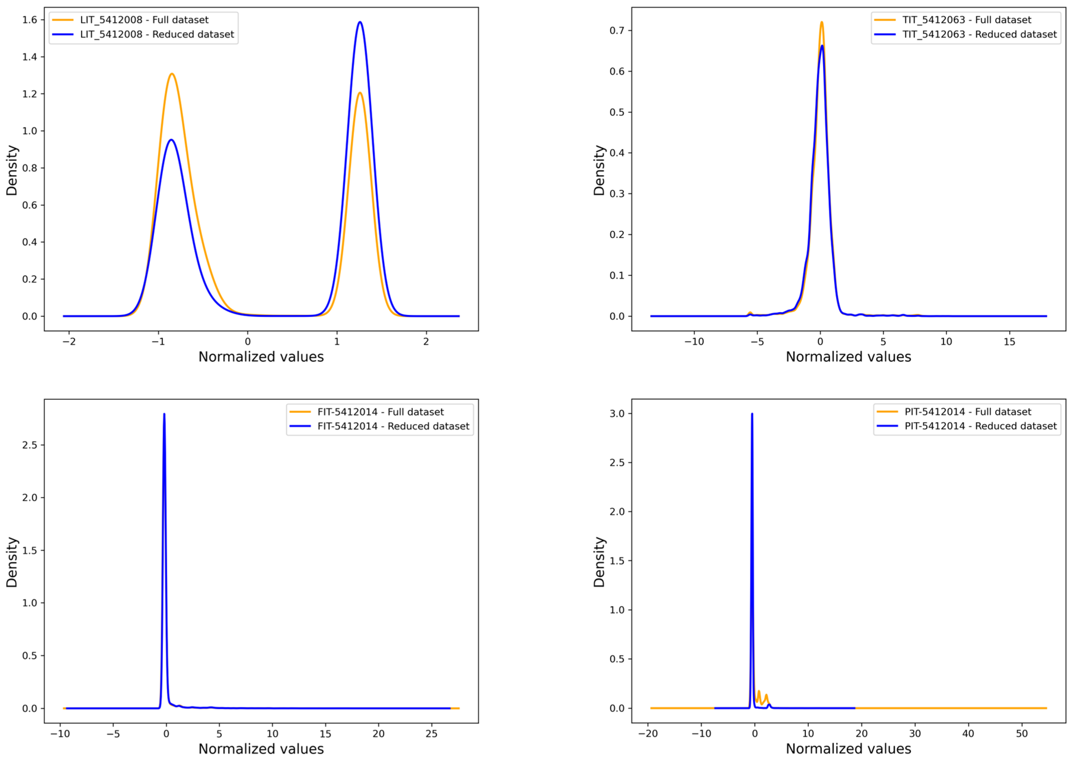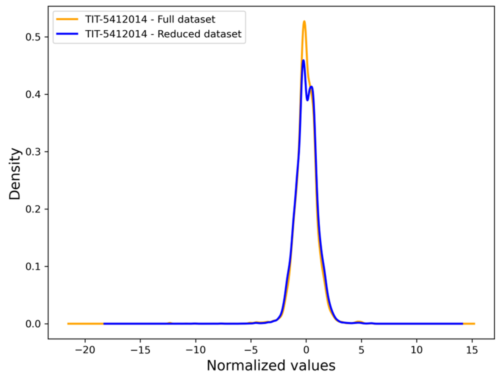Figure 10 shows the density distributions of the five features from the two datasets: the full dataset and the reduced dataset obtained through ISLib. Despite the reduction in data volume, the distributions of the reduced dataset closely align with those of the original dataset across all features. This indicates that the Instance Selection process effectively retained the essential characteristics of the data while reducing their size and noise. The similarity in distribution ensures that the reduced dataset remains representative of the original dataset, preserving its statistical properties and integrity for subsequent analysis or modeling.

The overall analysis by ISLib, in this case, took 7 s to converge in an Intel (R) Core (TM) i7-12800H 2.40 GHz with 32 GB RAM, speeding a process that would otherwise require long mining through historical data trends and information from different sources such as shutdown occurrences and maintenance registers.

After the two sequential analyses from ISLib, the resulting dataset comprised 20,809 observations, a reduction of 32% from the initial size. Both datasets were then used to train two AE networks. In order to compare the best possible models generated from each dataset, a hyperparameter tuning procedure was conducted separately using the Python framework Optuna 3.6.1 [53].

The Optuna’s hyperparameter selection process involves employing the Tree Parzen Estimator (TPE), a Bayesian-inspired sequential optimization method [54]. TPE reduces computational effort by minimizing the number of objective function evaluations, enabling real-time implementations. It formulates hyperparameter selection as an optimization problem, aiming to minimize the objective function evaluated on a validation set. This task becomes computationally challenging for models with numerous hyperparameters, such as neural networks. The TPE method addresses this issue by utilizing a surrogate objective function to approximate the true objective function. By iteratively maximizing the surrogate function, TPE identifies promising hyperparameter regions. The values with the highest surrogate function, called Expected Improvement, indicate regions for minimizing the original objective function. The probabilities of the surrogate model are updated accordingly, and the process continues until convergence or satisfactory hyperparameter values are found. SMBO/TPE reduces computational costs and has advantages like parallelizability and implementation in accessible numerical libraries [53,55]. For more information on TPE and the application of the Optuna framework to industrial process models, one should refer to the works of Bergstra et al. (2011) [54] and Lemos et al. (2021) [18], respectively. For the present study, the hyperparameter tuning process using Optuna focused on optimizing key parameters for each model. For AE, parameters such as the number of hidden layers, activation functions, and learning rates were optimized. For ESN, presented in the next section, the reservoir size, spectral radius, and input scaling were fine-tuned to enhance predictive performance.

Hyperparameter tuning took 6968 s for the full dataset and 4838 s for the reduced dataset. The performance of the two AE models during an online monitoring period with abnormal events is illustrated in Figure 11. All SPE values are normalized by their respective threshold (SPE_lim). As observed, during normal operation from the flare system, both models exhibit similar responses, with the AE generated using the reduced dataset displaying slightly lower reconstruction errors. During the abnormal events, both AE consistently show an increase in SPE values. However, since the model trained with selected instances appeared to be more sensitive to the presence of anomalies, as indicated by the higher peaks above the threshold limit, some of the faulty operations, such as the one observed on November 15th, could only be detected using the dataset provided by ISLib.

Figure 12 illustrates the same results as shown in Figure 11 while also presenting the corresponding trends from three of the features used as inputs for the models as obtained from historical operational data. It can be observed that a typical failure mode consists of a depressurizing event, indicated by the sudden increase in the pressure curve (depicted in blue), that is somehow not followed by a corresponding change in volume flow (the black line in the features trends). In such abnormal cases, the signal from the flowmeter either remains at zero or stays constant at some level below the expected value, given the behavior of the other features. This difference between the expected values from the AE model and the actual measured flow results in the high SPE shown in Figure 12. In this case, the reduced AE model successfully detected all the faulty operations while maintaining a low number of false positive alarms.

Figure 12 demonstrates the reduced AE model’s effectiveness in anomaly detection, notably in identifying discrepancies between pressure increases and stagnant volume flow rates. The reduction in dataset noise allows the AE to capture critical signal divergences more precisely, enabling earlier and more accurate fault detection compared to models trained on the complete dataset.

4.4. Oil Flowmeter

Fiscal meters are one of the most crucial pieces of equipment in an oil production platform, since they are directly related to royalties, allocation, and custody transfer calculations [21]. Measurement errors in these pieces of equipment can cause potential penalties and significant financial losses [56]. Because of that, regulatory bodies of concession or sharing contracts set guidelines to help the field operators ensure complete and accurate results [57]. In Brazil, for instance, ANP has strict procedures and protocols that must be followed in case of abnormalities such as incorrect measurement and configuration errors [21].

In order to minimize downtime and ensure the uninterrupted operation of an oil fiscal meter in one of Petrobras’ platforms, a monitoring system was created considering data from other instruments in the process plant, such as temperatures and pressures, to accurately predict the oil volume flow. The initial dataset consisted of nine features and 53,309 observations from months of operation obtained from historical operational data.

Figure 13 presents the results obtained from the batch instance selection step from ISLib. It is important to notice that, in this case, since the objective of the application was to produce a supervised model for a soft sensor, the supervised option was also applied in ISLib, meaning that, differently from the previous two cases, the results shown here were generated by a Regression Tree (RT) model instead of the unsupervised PCA approach.

Following a similar approach to the one described in the previous section, the monitoring team decided to keep only the highest-ranked cluster for the remaining steps by examining the operating modes. This was because all the other regions seemed to show some undesirable characteristics, such as measurement errors, plant shutdowns, etc., being thus classified as a different cluster by ISLib.

Figure 14 shows the enlarging windows analysis using the previously selected region (Cluster 0) as input. The results along the 100 intervals in the x-axis showed three pronounced drops in the MSE values in the first half of the dataset. This shows that the enlarging window procedure could outline subregions within the cluster analysis.

Preserving the data prior to the red circle in Figure 14, i.e., before the point at which the MSE reaches its minimum value, resulted in a dataset with 20,275 observations, a 62% reduction compared to the original dataset size of 53,309.

Using the previous methodology, the supervised model training was preceded by hyperparameter tuning in Optuna to obtain the best configuration for each ESN model. The total time required for optimization was 4229 s for the full dataset and 739 s for the reduced dataset.

Both trained neural network models were deployed using the SmartMonitor platform and consistently provided accurate predictions for the oil volume flow. Figure 15 depicts the predicted values of both models plotted against the real measured oil volume flow during a selected test period. The scatterplot on the right side displays a higher concentration of points around the identity line during normal operation, whereas a more dispersed distribution is found for extreme values. Interestingly, this behavior persists even for the ESN model trained on all operational regions.

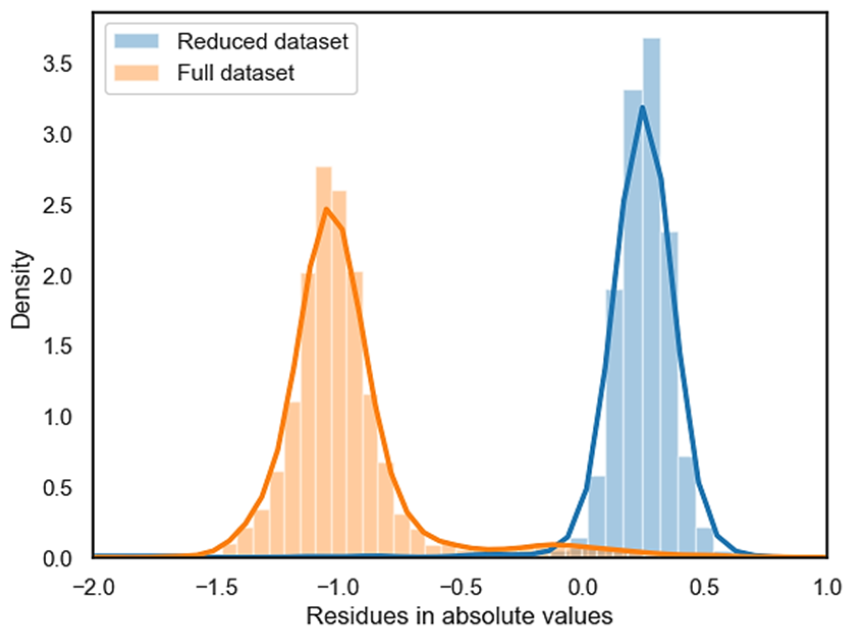
Figure 16 shows the residue distribution of the models during the same test period. As can be seen, both distributions show small offsets from zero. Notably, the ESN trained with only 38% of the original dataset presented better results, as evidenced by the higher concentration of residues closer to zero compared to the ESN trained with the whole dataset. The reduced dataset performs well due to the elimination of noisy and redundant data points, which enhances the model’s ability to generalize.

5. Conclusions

The importance of a proper instance selection procedure for regression problems was presented for real industrial settings, emphasizing the critical yet often overlooked step of data reduction in process monitoring frameworks and demonstrating how instance selection can significantly impact model performance in real-world scenarios. By employing a two-stage approach—unsupervised clustering to identify operational regions and an enlarging window strategy to determine the optimal training dataset size—the methodology tested, ISLib, demonstrated its ability to improve model performance while significantly reducing dataset size. The methodology for instance selection was evaluated in three distinct cases, covering a range of applications with specific goals, allowing the proposed procedure to be tested in various scenarios, including (i) independent evaluation of the two methodologies that constitute the library, (ii) application in a real fault detection case, (iii) application in a real soft-sensor generation case, and (iv) utilization of the results for training different data-driven models encompassing both supervised and unsupervised approaches. Furthermore, the impact of incrementally larger datasets on the execution time of ISLib was also quantified. It was shown for the first time, and using real-world data from the oil and gas industry, that smaller datasets not only accelerated the training process, but also generated models that performed equally to or better than their counterparts trained with the full-size dataset. This challenges the traditional assumption that larger datasets always result in better regression models, highlighting the critical role of thoughtful data reduction in capturing relevant behaviors while eliminating noise and redundancies.

Table 6. Summary of the results obtained for the evaluated cases.

Dataset	Objective	Model (h)	Dataset Initial Size (M)	Dataset Final Size (S)	Training Time Reduction [%]	Instance Selection Analysis Time [s]
TEP	Unsupervised model	Principal Component Analysis (PCA)	500	340	10	3
Gas flowmeter	Unsupervised model	Autoencoder (AE)	30,775	20,809	30	7
Oil flowmeter	Supervised model	Echo State Network (ESN)	53,309	20,275	82	17

complements the information provided in Table 1 by adding the results obtained from ISLib for each evaluated case. Notably, a significant reduction in model training time was observed for both industrial cases. Moreover, it is worth noting that ISLib was able to complete its analysis in less than 20 s, even for the largest evaluated dataset. This performance can be attributed to the utilization of robust and fast-converging algorithms such as PCA and Regression Trees, as well as the incorporation of the K-Means technique for identifying operational regions. Based on the results obtained, it can be concluded that any potential gains in accuracy achieved using more powerful techniques were outweighed by the speed and responsiveness of the proposed methodology. The obtained results highlight the importance of a proper instance selection—even in regression problems—and encourage the adoption of simple and efficient solutions that deliver valuable insights to end-users in complex industrial environments.

Looking ahead, future research should focus on refining and expanding ISLib’s methodology to handle datasets with more complex or dynamic characteristics. For example, advanced clustering techniques, such as DBSCAN, or hybrid approaches integrating temporal dependencies could be explored to improve operational region segmentation. Although ISLib demonstrated good efficiency, computational scalability challenges related to large datasets need to be addressed for broader applicability. Investigating computational optimizations for high-dimensional datasets will be key to its integration into diverse industrial contexts. Additionally, benchmarking ISLib against other regression-focused instance selection methods [29,32,58], as well as testing it on datasets from different industries, will further validate its robustness and uncover opportunities for methodological improvements.