A Study on Ejector Structural and Operational Conditions Based on Numerical Simulation

Abstract

The Shenfu Gas Field faces challenges with uneven wellhead pressures, where low-pressure wells lose discharge capacity and high-pressure wells require throttling, leading to significant energy waste. Ejectors offer potential for energy recovery by utilizing high-pressure gas to boost low-pressure production. A computational fluid dynamics (CFD) model was developed using simulation software to simulate ejector performance. Parametric studies analyzed key structural parameters (mixing chamber length L_m, diameter D_m, nozzle spacing L_c, diffuser length L_d) and operational variables (compression ratio, working/entrained fluid pressures). Model validity was confirmed via grid independence tests and experimental comparisons (error < 10%). Network-level efficacy was verified using pipeline simulation software. Entrainment ratio (ε) and isentropic efficiency (η) exhibited non-linear relationships with structural parameters, with distinct optima depending on compression ratio. D_m had the strongest influence on ε. Higher compression ratios reduced ε, while increasing working fluid pressure or entrained fluid pressure improved ε. Optimal configurations were identified. Network simulations confirmed functional effectiveness, though efficiency diminished over production time. Ejector efficiency is highly sensitive to specific structural and operational parameters. Deployment in gas gathering networks is viable but most beneficial in early production stages.

1. Introduction

With the development of the global economy and social progress, the demand for natural gas, a high-quality clean energy source, has increased dramatically. Since global conventional oil and gas resources account for only one-fourth of the reserves of unconventional oil and gas resources, conventional natural gas alone cannot meet social needs. Thus, the focus of global natural gas exploration and development has gradually shifted from conventional to unconventional natural gas. Coalbed methane, tight gas, and shale gas all belong to unconventional natural gas. As their reservoirs are all coal-measure source rocks, they are collectively referred to as the “three coal-measure gases,” with reserves approximately 1.96 times those of conventional natural gas, occupying a primary position in unconventional natural gas. The Shenfu Gas Field, recognized as one of China’s pivotal unconventional gas reservoirs, possesses substantial resource reserves. However, its development faces technical challenges including numerous wellheads, uneven pressure distribution across the field, and declining formation pressures in certain gas wells over production time. Notably, when wellhead pressures fall below the inlet pressure threshold of gathering stations, low-pressure gas wells lose effective discharge capacity, while high-pressure counterparts require throttling treatment for integration into the gas gathering system [1]. This operational paradox presents a critical opportunity: harnessing the expansion energy from high-pressure gas wells to drive production enhancement and transportation of low-pressure gas. Implementing such energy coupling technology could substantially mitigate resource waste while generating remarkable economic returns and environmental benefits through optimized energy utilization.

As a fluid dynamic device for pressurization and transportation, ejectors utilize high-pressure gas well energy to boost low-pressure wells, thereby entraining and enhancing production from depleted gas reservoirs. Owing to their structural simplicity and operational flexibility, ejectors have been extensively investigated and deployed across multiple engineering domains. Contemporary research methodologies predominantly integrate numerical simulation with experimental validation.

Tomasz Kuś et al. [2,3,4] pioneered numerical analysis using CO₂ as the working fluid to elucidate its inhibitory effects on condensation during ejector operation. Bingyuan Hong et al. [5] developed a steady-state hydraulic model for natural gas pipeline networks incorporating pressure-exchange ejectors by coupling ejector characteristic equations with pipeline hydraulic behavior. Substantial efforts have focused on optimizing ejector efficiency through geometric modifications and operational adjustments. For instance, Xiaolei Zhang [6] employed gas dynamic function theory combined with numerical and experimental approaches to refine structural parameters for enhanced performance. Similarly, Zhe Zhang and Xiujuan Chen [7,8] systematically evaluated the influence of critical dimensional parameters on ejector efficiency using computational fluid dynamics (CFD) simulations. Yuyan Hou et al. [9] established a 3D CFD model to determine optimal mixing chamber lengths under varying operational parameters. Xin Jin [10] investigated ejector entrainment performance for low-pressure coalbed methane through multi-scenario simulations.

Innovative configurations beyond conventional designs have also emerged. Shuang Mei [11] proposed an ejector architecture tailored for natural gas liquefaction cycles, analyzing efficiency variations under structural and operational perturbations. Jingming Dong et al. [12] conducted the first systematic study on performance degradation caused by primary nozzle misalignment due to installation errors or vibration. Amer Muzaber et al. [13] introduced a breakthrough design featuring an arc-shaped mixing chamber, overcoming limitations of traditional linear geometries. Huadong Liu et al. [14] numerically examined flow field evolution and performance metrics of a novel ejector incorporating a straight-tube extension at the working nozzle outlet. These advancements collectively provide critical insights for optimizing ejector efficiency and guiding future research directions.

This study systematically investigates the operational mechanisms of ejectors through comprehensive analytical methods. A computational fluid dynamics (CFD) model was developed using ANSYS Fluent 2024 to evaluate ejector efficiency variations under modified structural parameters and operational conditions. Through parametric analysis, the optimized dimensions of the key structural parameters of the ejector and their applicable operating conditions were determined, and the effectiveness of installing the ejector in the pipeline network was verified using self-developed software. These findings establish operational guidelines for ejector deployment strategies and applicability boundaries, providing actionable insights for field implementation.

2. Materials and Methods

2.1. Ejector Design

2.1.1. Governing Equations

The numerical simulation of fluid dynamics within the ejector was performed using ANSYS Fluent 2024, requiring solutions to the fundamental conservation equations: continuity, momentum, and energy equations. Given the compressible gas medium employed in this study, the governing equations are formulated as follows [1]:

Continuity Equation:

$${\displaystyle \frac{\partial \rho }{\partial t}}+{\displaystyle \frac{\partial \left(\rho u_i\right)}{\partial x_i}}=0$$

(1)

Momentum Equation:

$${\displaystyle \frac{\partial \left(\rho u_i\right)}{\partial t}}+{\displaystyle \frac{\partial \left(\rho u_i{u}_j\right)}{\partial x_i}}=-{\displaystyle \frac{\partial p}{\partial x_i}}+{\displaystyle \frac{\partial {\tau }_{ij}}{\partial x_i}}$$

(2)

Energy Equation:

$${\displaystyle \frac{\partial \left(\rho E\right)}{\partial t}}+{\displaystyle \frac{\partial \left[u_i\left(\rho E+p\right)\right]}{\partial x_i}}=\nabla ·\left({\displaystyle \frac{{\alpha }_{eff}\partial T}{\partial x_i}}\right)+\nabla ·\left[u_j\left({\tau }_{ij}\right)\right]$$

(3)

$${\tau }_{ij}={\mu }_{eff}\left({\displaystyle \frac{\partial u_i}{\partial x_j}}+{\displaystyle \frac{\partial u_j}{\partial x_i}}\right)-{\displaystyle \frac{2}{3}}{\displaystyle \frac{{\mu }_{eff}\partial u_k}{\partial x_k{\delta }_{ij}}}$$

(4)

In the formula:

t is time, s; ρ is the density, kg/m³; u is the velocity vector, m/s; p is the static pressure, Pa; T is the temperature, K; E represents the kinetic energy of the reflected object, m²/m²; τ is the stress tensor, Pa; α_eff is the thermal conductivity coefficient, W/(m·K); μ_eff is the dynamic viscosity, Pa·s; δ_ij is the Kronecker delta function.

2.1.2. Performance Evaluation Metrics

As established in the seminal work by Sokolov et al. [15], the operational performance of ejectors is primarily evaluated through the entrainment ratio (ε), defined as the mass flow rate ratio between the entrained (low-pressure) fluid and the primary (high-pressure) working fluid:

$$\epsilon ={\displaystyle \frac{M_l}{M_h}}$$

(5)

In the formula, M_l and M_h represent the mass flow rates of the low-pressure fluid and the high-pressure fluid, respectively.

The entrainment process in an ejector can be thermodynamically characterized as follows: the low-pressure fluid is compressed to an intermediate pressure, thereby gaining energy, while the high-pressure fluid expands to the same intermediate pressure, releasing energy. The energy acquired by the low-pressure fluid originates entirely from the energy released by the high-pressure fluid, with higher energy transfer efficiency correlating directly to improved ejector performance. Assuming both energy gain (compression) and release (expansion) processes approximate isentropic transformations, the work contributions of the high- and low-pressure gases during entrainment can be theoretically estimated. To more accurately evaluate ejector performance, this study introduces isentropic efficiency (η) as a secondary performance metric, referencing the methodology of Peiqi Liu et al. [16]. The calculation is defined as follows:

$$\eta ={\displaystyle \frac{W_l}{W_h}}={\displaystyle \frac{\left(M_l\times T_l\times \left({\left(\frac{P_m}{P_l}\right)}^{\frac{k-1}{k}}-1\right)\right)}{\left(M_h\times T_h\times \left(1-{\left(\frac{P_m}{P_h}\right)}^{\frac{k-1}{k}}\right)\right)}}$$

(6)

In the formula: W_l and W_h represent the work carried out by the absorption and release of energy by low-pressure and high-pressure gases, respectively; M_l and M_h are the mass flow rates of low-pressure and high-pressure gases, respectively; T_l and T_h are the temperatures of low-pressure and high-pressure gases, respectively; P_m, P_l, and P_h are the pressures of medium-pressure, low-pressure, and high-pressure gases, respectively; k is the adiabatic index of the gas.

2.1.3. Ejector Geometric Design

The ejector configuration employed in the simulations is illustrated in Figure 1, comprising four critical functional components: fluid inlets/outlets, nozzle, mixing chamber, and diffuser.

The specific structural dimensions of the ejector were primarily determined based on technical commissioning requirements, while other unspecified parameters were derived from empirical formulas proposed by Sokolov in his seminal work [17]. To optimize the key structural parameters of the ejector, this study focuses on four critical design variables for simulation analysis: mixing chamber length (L_m), mixing chamber diameter (D_m), nozzle axial spacing (L_c), and diffuser length (L_d). Detailed parameter specifications are provided in

Table 1. Key structural dimensions of the ejector.

Parameter	Lc/mm	Dm/mm	Lm/mm	Ld/mm
Numerical value	12–24	20–62	120–300	283.65–834.55

.

2.2. Ejector Model Development

2.2.1. Model Construction and Grid Discretization

The ejector model was established based on the finalized dimensional design parameters. To leverage structural symmetry and simplify computational analysis, an axisymmetric configuration was adopted, with numerical calculations performed on a half-cross-sectional domain.

For grid generation, quadrilateral-dominant meshing was employed due to the geo-metric regularity of the ejector. Critical attention was paid to grid density optimization: excessively coarse grids may induce convergence failures, while overly refined grids risk computational instability due to excessive node counts. Through grid independence verification, a balanced cell size of 0.5 mm × 0.5 mm was selected to ensure numerical accuracy and solution robustness. The computational domain and meshing scheme are illustrated in Figure 2.

2.2.2. Boundary and Solver Configuration

In the simulation process of this paper, a steady-state calculation for a static ejector was adopted. Since the parameters of coal-bed methane and tight gas provided are not significantly different, for the convenience of subsequent simulation calculations, tight gas was selected as the simulation medium, and its specific components are shown in

Table 2. Components of tight gas.

Component	Methane	Ethane	Propane	Isobutane	N-Butane	Isopentane	N-Pentane	Nitrogen gas	Carbon Dioxide
Proportion/%	87.3883	5.4167	0.7533	0.1167	0.125	0.045	0.0317	0.21	5.92

. As the pressure magnitude of the boundaries set in the simulation process is in the order of megapascals, the compressibility of the gas medium cannot be ignored. Therefore, to ensure the accuracy of the calculation, a density-based solver was selected. Regarding the influence of pressure and temperature on the density of gas media, prior to setting gas parameters in the simulation, this study performed calculations using physical property calculation software to obtain the thermophysical properties of the gas medium under specified pressure and temperature conditions. Gas parameters were then set based on the calculated data. The specific parameter calculation results are shown in

Table 3. The physical properties of gas media under specific pressure and temperature conditions.

Pressure (MPa)	Temperature (K)	Molar Density (kgmole/m3)	Mass Density (kg/m3)	Mass Heat Capacity (kJ/kg-C)	Thermal Conductivity (W/m-K)	Viscosity (cP)
10	288.15	5.578	105.6	3.061	0.04322	0.015
4	288.15	1.911	36.17	2.320	0.03351	0.0119
1.7	280.65	0.7716	14.61	2.098	0.03035	0.0111
1.7	288.15	0.7478	14.16	2.106	0.03133	0.01135

.

Since the designed numerical model has a two-dimensional axisymmetric structure and the boundary pressure is relatively high, and the performance of the ejector is sensitive to the turbulence model [18], the realizable k-ε turbulence model was chosen and coupled with a two-dimensional axisymmetric eddy current solver for the solution operation.

The high-pressure and low-pressure gas inlets were set as pressure inlets, and the medium-pressure gas outlet was set as a pressure outlet. Specifically, the high-pressure was set at 10 MPa; the low-pressure was set at 4 MPa; and the compression ratios were 1.2, 1.5, and 2.0. The specific settings are shown in

Table 4. Settings of pressure inlet.

Entry Type	Reference Frame	Net Total Pressure	Initial Static Pressure	Direction Specification Law	Turbulence Intensity	Turbulent Viscosity Ratio
High-pressure inlet	Absolute mode	10	10	Perpendicular to the boundary	5%	1
Low-pressure inlet	Absolute mode	4	4	Perpendicular to the boundary	5%	1

and

Table 5. Settings of Medium Voltage Outlet.

Entry Type	Reference Frame	Compression Ratio	Net Total Pressure	Direction Specification Law	Turbulence Intensity	Turbulent Viscosity Ratio
Pressure outlet	Absolute mode	1.2	4.8	Perpendicular to the boundary	5%	1
		1.5	6
		2.0	8

. For the wall boundary, an adiabatic no-slip wall boundary was selected.

The numerical solver configuration was meticulously designed to balance computational convergence and solution accuracy through two critical aspects:

Residual Convergence Criteria: Convergence thresholds were rigorously set at a residual level of 10⁻⁶ for all governing equations (continuity, momentum, energy, and turbulence quantities), ensuring solution fidelity comparable to experimental uncertainties.

Solver algorithm settings: as detailed in

Table 6. Settings of the solution process.

Equation	Flux Type	Gradient	Turbulent Kinetic Energy	Flow	Turbulent Dissipation Rate
Implicit	Roe-FDS	Green-Goss is based on the unit	Second-order upwind format	Second-order upwind format	Second-order upwind format

[18].

2.2.3. Model Validation

Grid Independence Verification

When the grid density varies, the simulation results differ under identical parameter conditions. Generally, as grid density increases, the accuracy of the simulation results improves. However, once the grid density reaches a certain threshold, its impact on the simulation results becomes negligible. At this point, it can be concluded that the influence of grid count on the simulation results is minimal. This study compared the ejector coefficients of four models with different mesh densities under consistent parameter settings. The error terms in

Table 7. Comparison of ejection coefficients under different grid numbers.

Number of Grids	Ejection Coefficient	Error
21,450	0.6521	--
33,206	0.6965	6.8%
48,740	0.7324	5.2%
59,560	0.7416	1.3%

represent the errors between simulation results of different groups, specifically the relative errors obtained by comparing the simulation results of each group with those of the previous group. When the number of meshes is 59,560, the simulation results are close to those when the number of meshes is 48,740, with an error of 1.3%. Consequently, it can be reasonably inferred that at a grid count of 59,560, further increases in grid density do not significantly affect the computational outcomes.

Model Rationality Validation

To verify the correctness of the simulation model in this paper, the experimental data from Reference [19] were adopted, and the simulation results of the model in this paper were compared with the experimental data under the same working conditions.

Table 8. Experimental working conditions.

Serial Number	High-Pressure Inlet		Low-Pressure Inlet		Medium-Pressure Outlet
	Pressure (MPa)	Temperature (°C)	Pressure (MPa)	Temperature (°C)	Pressure (MPa)
1	9.915	29.9	3.996	17.4	4.38
2	8.668	33.4	3.652	6.6	4.072
3	9.091	26.7	3.595	7.6	3.873
4	9.850	35.5	5.149	20.7	5.560
5	9.455	36.3	4.761	15.1	5.179
6	8.846	35.6	4.255	13.7	4.667

shows the experimental working condition parameters, and Table 8 presents the comparison between the simulated values and experimental values under corresponding working conditions. The error values listed in

Table 9. Comparison of simulation and experimental results.

Serial Number	Experimental Result	Simulation Result	Relative Error
	Ejection Coefficient	Ejection Coefficient
1	0.6742	0.7416	9.99%
2	0.5723	0.6121	6.95%
3	0.5568	0.5928	6.47%
4	0.5674	0.5947	4.81%
5	0.4553	0.4874	7.05%
6	0.4003	0.4268	6.62%

denote relative errors between simulation outcomes derived from the experimental parameters of Ref. [19] and the corresponding experimental data documented therein. These errors are attributed to deviations between the structural parameters of the experimental setup and the parameters specified in the model. As indicated by the data in the tables, the errors between the simulation results of the model in this paper and the experimental results are within 10% under all groups of working conditions. Therefore, it can be roughly concluded that the calculation model in this paper is correct [20,21,22,23].

3. Results

3.1. Influence of Structural Parameters on ε and η

During the structural optimization simulation, the boundary conditions of the inlet and outlet were kept constant, and the simulation optimization was mainly carried out for key structural parameters such as the mixing chamber length L_m, mixing chamber diameter D_m, nozzle spacing L_c, and diffuser length L_d [24,25,26]. The single-variable principle was adopted in the simulation: only one parameter was analyzed each time, while other parameters were kept unchanged. By changing a single structural parameter and obtaining the corresponding simulation results, summary and analysis were conducted, and variation curves of ε and η under the change of a single structural parameter were plotted [27,28,29].

3.1.1. Mixing Chamber Length L_m

When studying the influence of the mixing chamber length variation on the entrainment efficiency, all other structural and operating parameters were kept constant to investigate the effect of L_m variation on the ejector’s performance under different compression ratios L_m.

Figure 3 and Figure 4 show the variation curves of the entrainment coefficient and isentropic efficiency with the mixing chamber length under different compression ratios. As indicated in the figures, under different compression ratios, both the entrainment coefficient and isentropic efficiency first increase and then decrease with the increase in L_m. When P_m/P_l = 1.2 and P_m/P_l = 1.5, the entrainment coefficient reaches its maximum value at L_m = 210 mm, which are 71.6% and 53.5%, respectively. However, when the compression ratio increases to 2.0, the entrainment coefficient peaks at L_m = 180 mm with a value of −7%. The variation trend of the peak value of isentropic efficiency is consistent with that of the entrainment coefficient. (Special note: Negative values of the ejector coefficient and negative isentropic efficiency are specifically manifested as negative outlet flow rates of the ejector, meaning that the energy carried by the mixed gas fails to overcome the outlet backpressure. As a result, the mixed gas cannot flow out of the outlet, causing a backflow phenomenon at the outlet. Negative ejector coefficients and negative isentropic efficiencies occur under the extreme boundary conditions simulated in this study. Such cases are theoretically valid, as evidenced by the negative ejector coefficients reported in Refs. [1,6,8,10]. All negative ejector coefficients and negative isentropic efficiencies presented in the subsequent content are simulation results under extreme boundary conditions).

When L_m is small, the gas is insufficiently mixed when flowing through the mixing chamber, and the mixing effect of the chamber is insignificant. This results in a low pressure level of the mixed gas when it reaches the diffuser; additionally, the pressure distribution of the mixed gas is uneven, with the axial pressure being lower than the wall pressure. These phenomena indicate that the momentum exchange between the working gas and entrained gas is insufficient at small L_m, which is numerically reflected by a small entrainment coefficient. As L_m increases, the gas mixing becomes more thorough, leading to a higher pressure of the mixed gas at the diffuser inlet. This enhances the gas’s ability to overcome backpressure, thereby improving the ejector’s performance under this pressure range and resulting in a larger entrainment coefficient.

However, as L_m increases, the contact area between the gas and the wall of the mixing chamber also increases. The high-speed flowing gas mixture generates greater shear stress with the wall. As the gas flows, this shear stress accumulates along the path to form frictional loss, which consumes the gas kinetic energy. The energy mainly originates from the energy transferred from the working gas to the entrained gas. Therefore, with the increase in L_m, the net kinetic energy carried by the entrained gas when leaving the mixing chamber continuously decreases, leading to a reduction in its capacity to overcome the backpressure at the diffuser outlet. This ultimately manifests as a decrease in the flow rate of the entrained fluid at the outlet, i.e., the decline in the working efficiency of the ejector. When L_m is excessively large, the frictional losses become dominant, reducing the energy absorbed by the entrained gas and causing insufficient momentum exchange. Therefore, an excessively large L_m will also lead to a decrease in the entrainment coefficient. Consequently, during the structural design of the ejector, the axial length of the mixing chamber should be reasonably selected to ensure optimal operational performance of the ejector.

3.1.2. Mixing Chamber Diameter D_m

To investigate the influence of the mixing chamber diameter D_m on the entrainment performance, all other structural parameters were kept constant, and the effects of different D_m values on the entrainment coefficient and isentropic efficiency were explored.

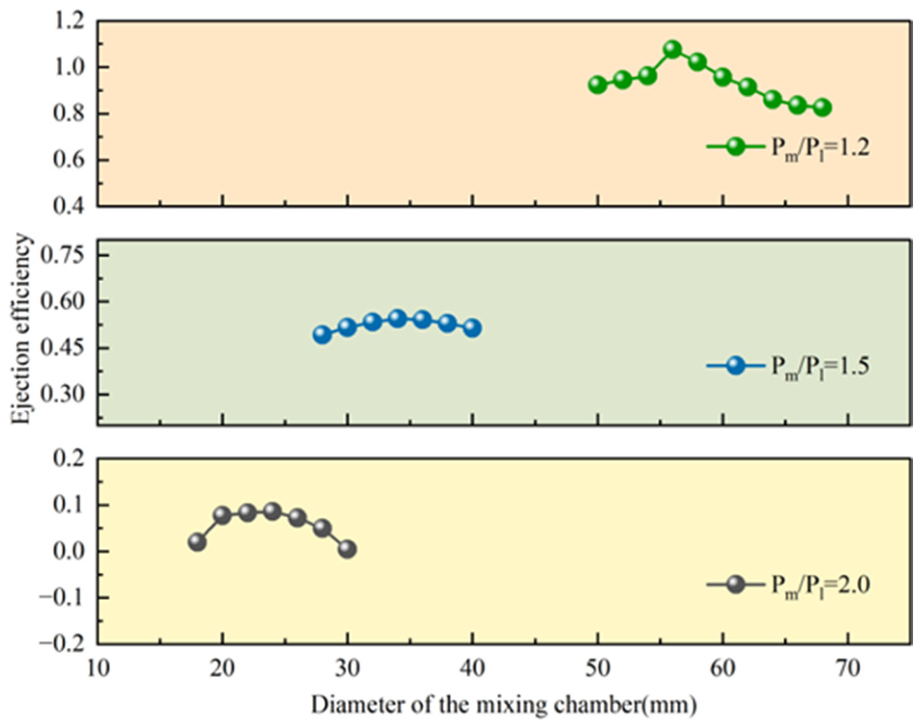
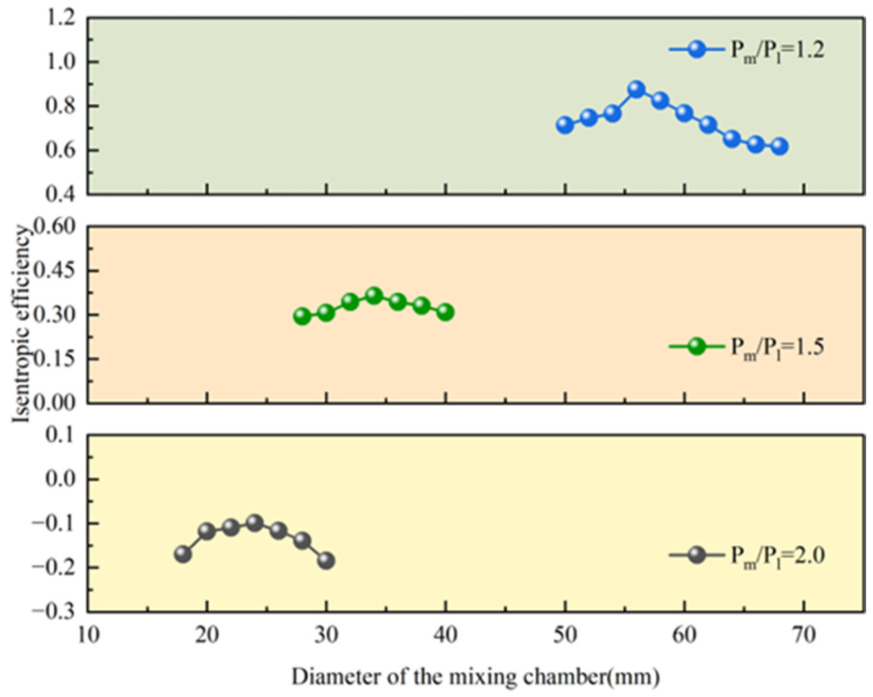
As shown in Figure 5 and Figure 6, under different compression ratios, the variation patterns of the entrainment coefficient and isentropic efficiency are basically identical when the mixing chamber diameter D_m changes, both exhibiting a trend of first increasing and then decreasing with the increase in D_m. When P_m/P_l = 1.2, the entrainment coefficient reaches its maximum value of 107.57% at D_m = 56; when P_m/P_l = 1.5, the maximum entrainment coefficient of 54.43% occurs at D_m = 34; when P_m/P_l = 2.0 and D_m = 24, the entrainment coefficient peaks at 8.58%. Under different compression ratios, the D_m values corresponding to the maximum isentropic efficiency are the same as those for the entrainment coefficient, but the numerical values are generally lower.

When D_m is small, the volume of the mixing chamber is limited, and the throttled working gas occupies the chamber upon arrival, causing congestion. As a result, only a small amount of entrained gas can enter the mixing chamber for momentum exchange, restricting the entrainment effect of the fluid and leading to a low entrainment coefficient. As D_m gradually increases, the flow cross-section of the working gas becomes smaller than that of the mixing chamber, allowing for more entrained gas to flow into the mixing chamber under the action of pressure difference, thereby increasing the entrainment coefficient. When D_m is excessively large, the flow rate of the entrained gas further increases. However, due to the low velocity of the entrained gas, it restricts the high-velocity working gas, resulting in a lower velocity and kinetic energy of the mixed fluid. Although the gas is well-mixed in this case, the significantly reduced velocity—combined with the influence of outlet backpressure—hinders the axial flow of the mixed fluid, forcing it to flow along the lower-pressure wall. Consequently, partial entrained gas undergoes backflow, leading to a decline in entrainment efficiency.

3.1.3. Nozzle Spacing L_c

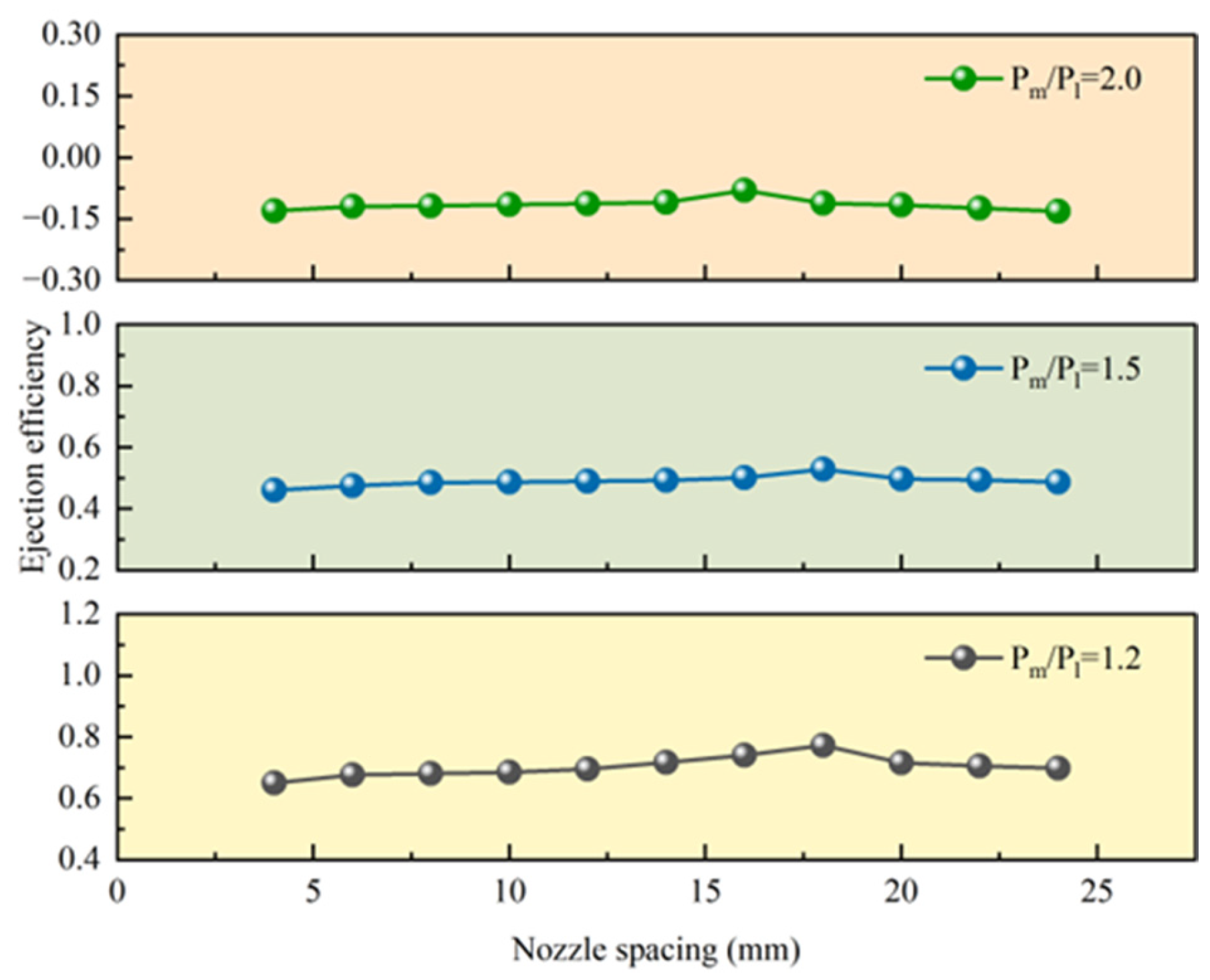
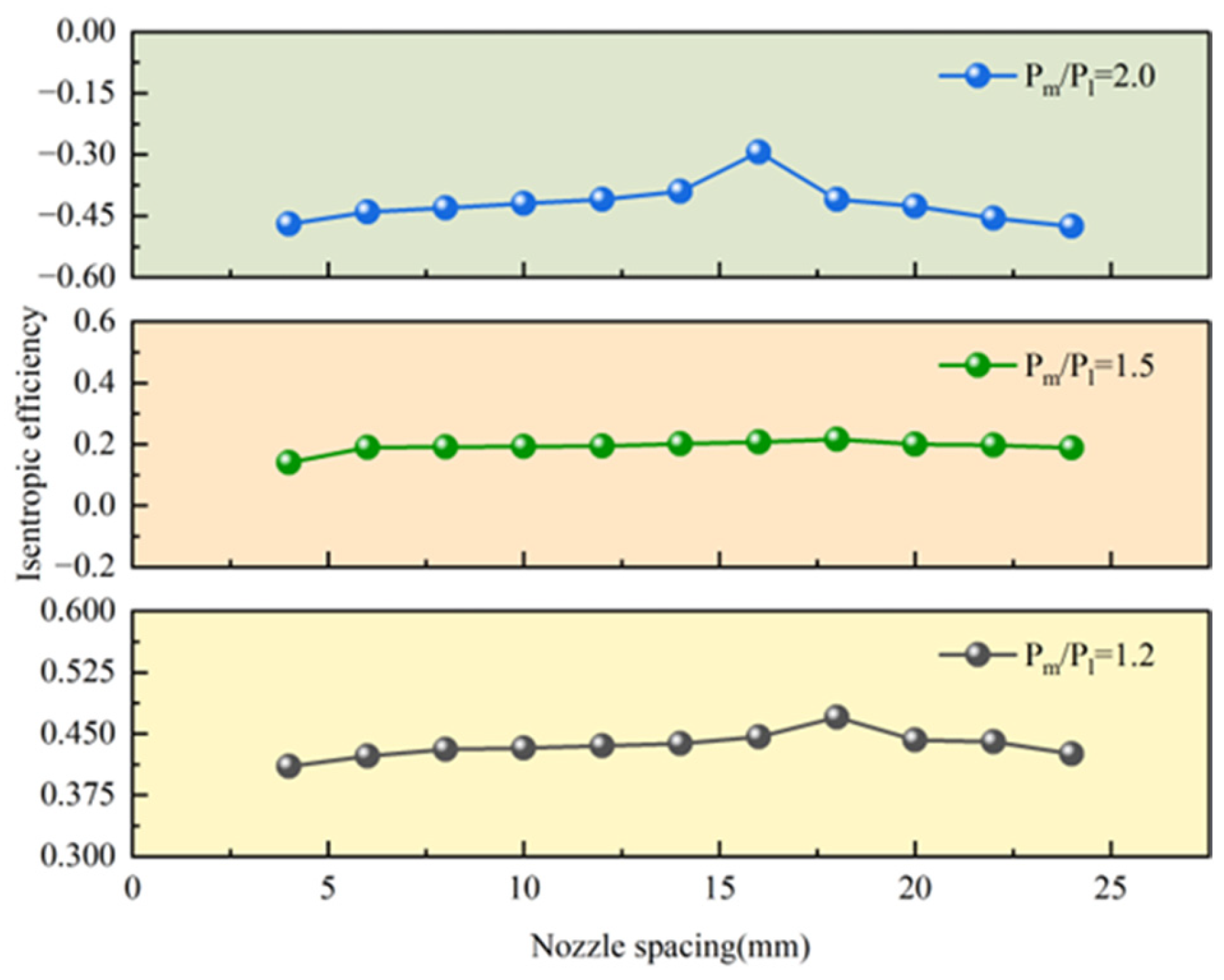
As shown in Figure 7 and Figure 8, when the nozzle spacing L_c changes, the entrainment coefficient and isentropic efficiency exhibit the same variation pattern: both first increase and then decrease with the increase in L_c. Under the compression ratios P_m/P_l = 1.2 and P_m/P_l = 1.5, the entrainment coefficient reaches its maximum value at L_c = 18 mm, with values of 77.2% and 52.8%, respectively. When P_m/P_l = 2.0, the entrainment coefficient peaks at L_c = 16 mm, with a value of −8.02%.

When L_c is small, the frictional resistance loss is low. However, in reality, the working fluid entrains the entrained fluid through shear forces generated by high-velocity flow. If L_c is too small, the working fluid lacks sufficient entrainment distance to drive the entrained fluid before reaching the mixing chamber, resulting in a low flow rate of the entrained fluid and thus a small entrainment coefficient. As L_c increases, the working fluid gains adequate entrainment distance to carry the entrained fluid, leading to an increase in the entrained fluid flow rate and consequently an increase in the entrainment coefficient. When L_c exceeds the critical value, further increases in L_c lead to higher frictional resistance losses, causing significant energy loss in the mixed fluid. Restricted by backpressure, the mixed fluid flows along the wall, inducing fluid backflow and reducing entrainment efficiency.

3.1.4. Diffuser Length L_d

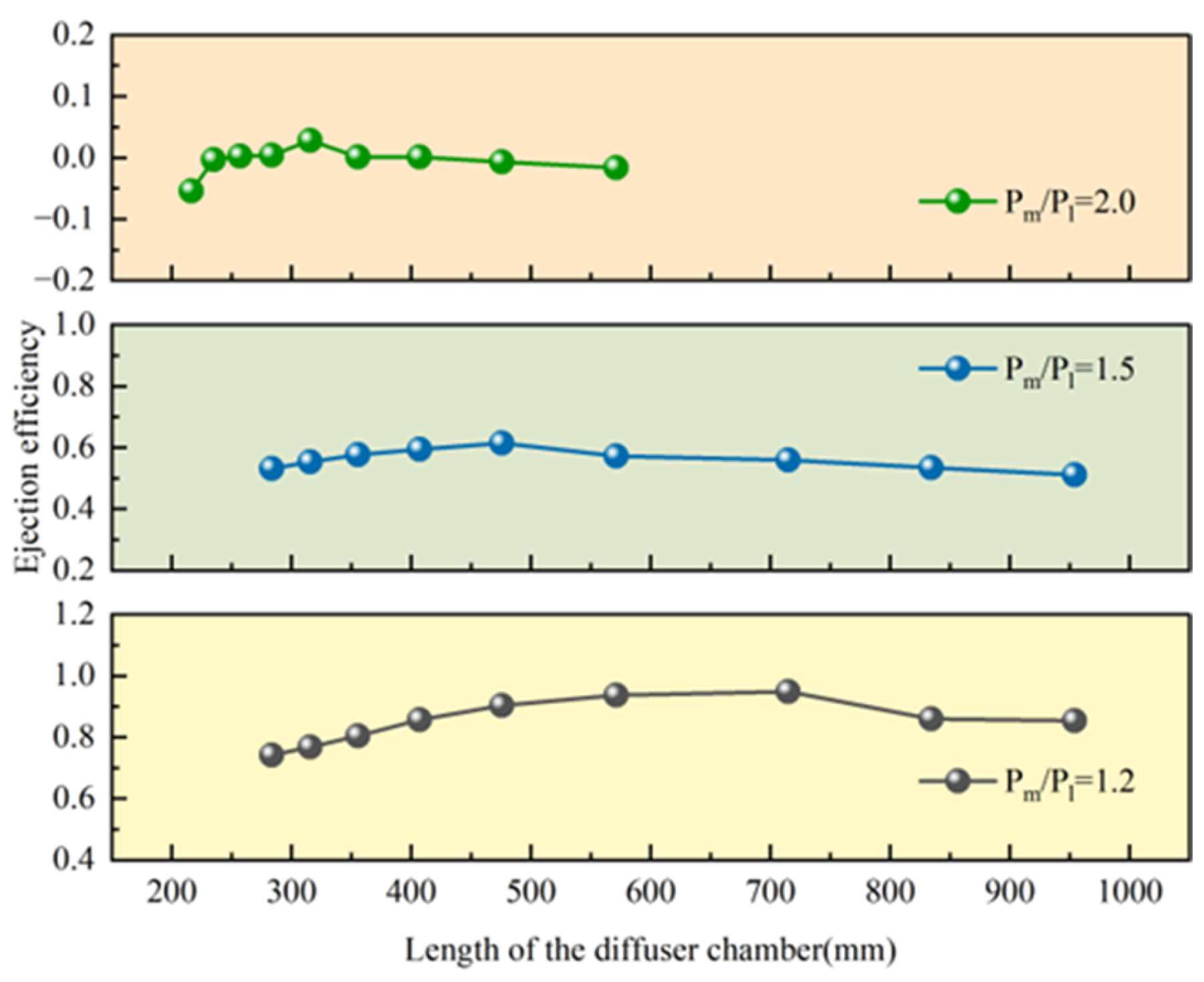
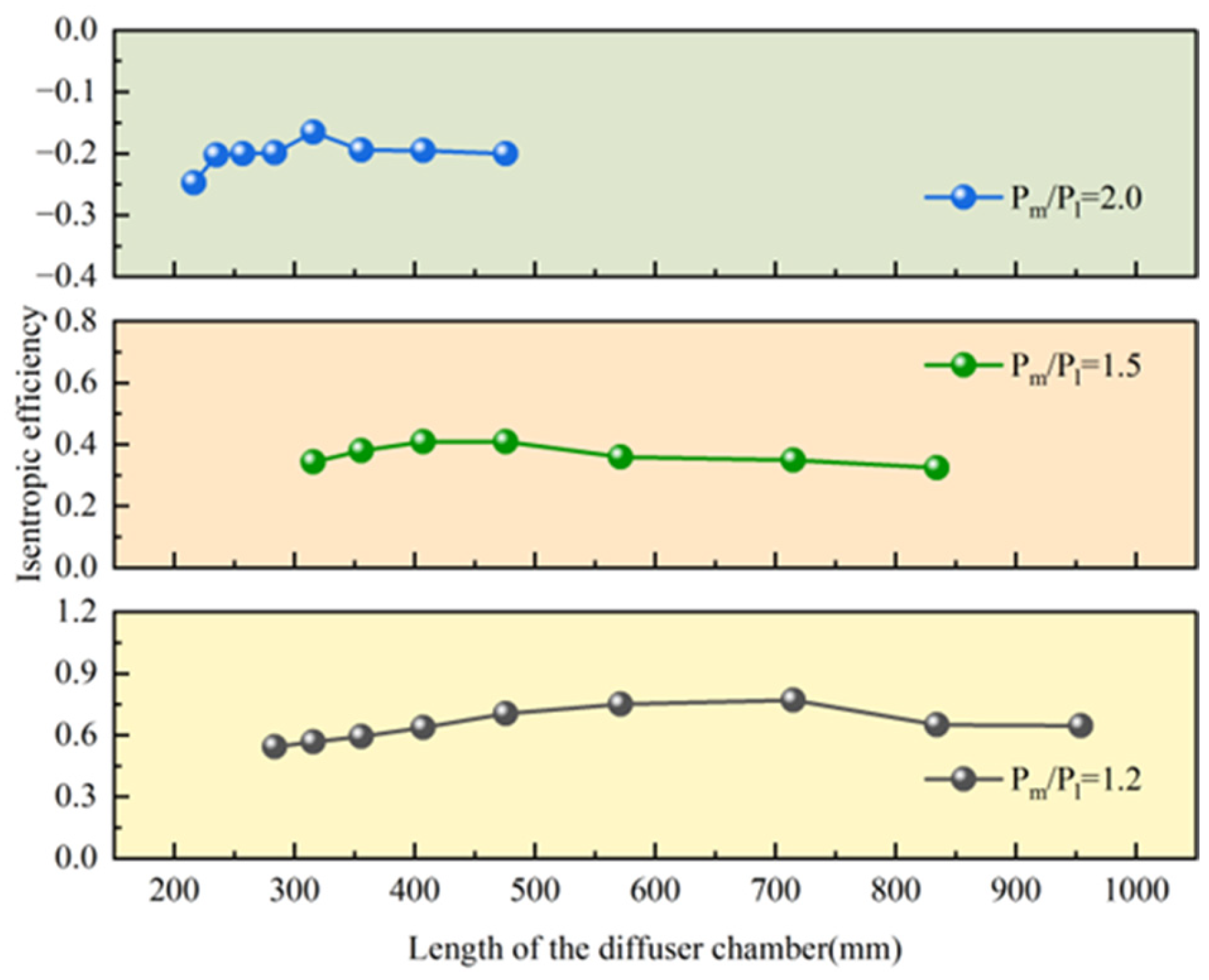
As shown in Figure 9 and Figure 10, both the entrainment coefficient and isentropic efficiency of the ejector exhibit a trend of first increasing and then decreasing with the increase in diffuser length L_d. When the compression ratio P_m/P_l = 1.2, the entrainment coefficient reaches its maximum value of 94.92% at L_d = 715.03 mm; under P_m/P_l = 1.5, the maximum entrainment coefficient of 61.43% occurs at L_d = 475.72 mm; when P_m/P_l = 2.0, the entrainment coefficient peaks at 2.8% with L_d = 315.69 mm.

After the working fluid and entrained fluid are thoroughly mixed in the mixing chamber, they enter the diffuser. When L_d is small, the mixed fluid experiences minimal deceleration and pressure increase in the diffuser, meaning the diffuser fails to fulfill its pressure-increasing function, resulting in low entrainment efficiency. As L_d increases, the diffuser provides sufficient distance for pressure buildup, thereby enhancing entrainment efficiency. However, when L_d exceeds the optimal value, the kinetic energy consumed by frictional resistance of the mixed fluid becomes excessively large. Under the influence of outlet backpressure, the fluid flows along the wall surface, causing partial backflow within the diffuser and reducing entrainment efficiency.

In summary, under different simulation conditions, the key structural parameters investigated in this study all have their optimal values. When P_m/P_l = 1.2, the maximum entrainment coefficient is achieved with L_m = 210 mm, D_m = 56 mm, L_c = 18 mm, and L_d = 715.03 mm. For P_m/P_l = 1.5, the optimal values of L_m, D_m, L_c, and L_d are 210 mm, 34 mm, 18 mm, and 475.72 mm, respectively. When P_m/P_l = 2.0 and the entrainment efficiency is maximized, the values of L_m, D_m, L_c, and L_d are 180 mm, 24 mm, 16 mm, and 315.69 mm, respectively.

3.2. Influence of Operating Parameters on ε

Regarding the impact of ejector operating conditions on its efficiency, this paper dis-cusses the effects from three aspects: performance variations in the ejector under different compression ratios, and the influences of pressure changes in the working fluid and entrained fluid on entrainment performance [30,31,32]. For the simulation of operating condition changes, the structural parameters of the model—mixing chamber length L_m, diameter D_m, nozzle spacing L_c, and diffuser length L_d—were set to 210 mm, 30 mm, 20 mm, and 283.65 mm, respectively.

3.2.1. Variation of Entrainment Efficiency Under Different Compression Ratios

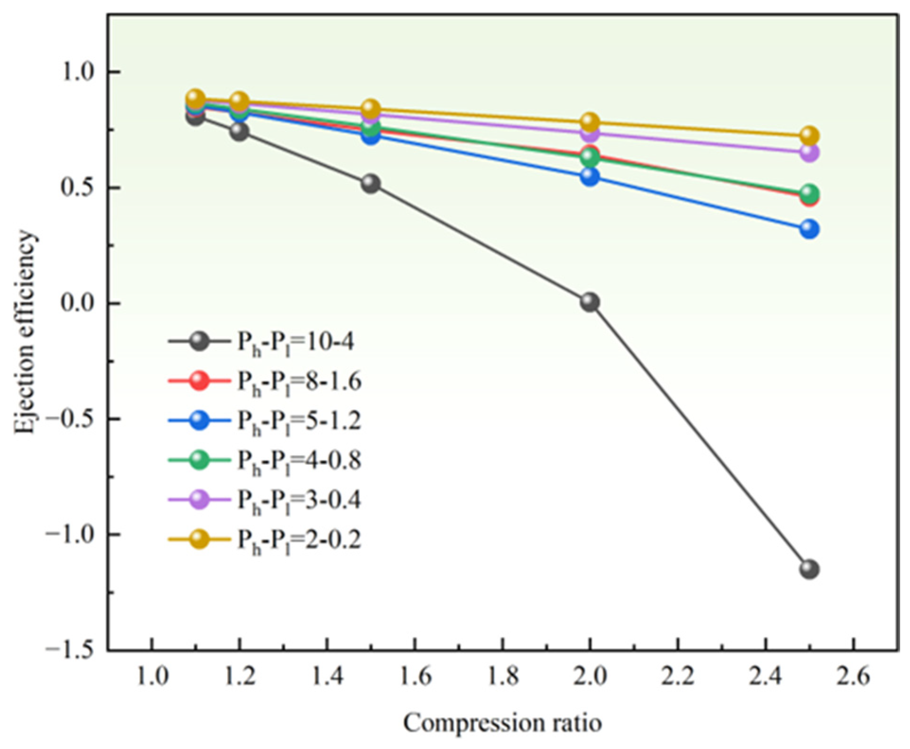
In this section of the simulation, six groups of different high-low pressure combinations were selected, and simulation results under five different compression ratios for each group were obtained to summarize and analyze the variation law of the entrainment coefficient. The specific parameters selected are listed in

Table 10. High- and low-pressure combinations and compression ratio selection.

High Pressure/MPa	Low Pressure/MPa	Compression Ratio
10	4	1.1/1.2/1.5/2.0/2.5
8	1.6	1.1/1.2/1.5/2.0/2.5
5	1.2	1.1/1.2/1.5/2.0/2.5
4	0.8	1.1/1.2/1.5/2.0/2.5
3	0.4	1.1/1.2/1.5/2.0/2.5
2	0.2	1.1/1.2/1.5/2.0/2.5

, and the simulation results are shown in Figure 11.

As shown in Figure 11, under different pressure combinations, the entrainment coefficient decreases with the increase in compression ratio. The maximum entrainment co-efficient of each group occurs at P_m/P_l = 1.1, while the minimum value occurs at P_m/P_l = 2.5.

Taking any pressure combination for analysis, changes in the compression ratio directly affect the ejector’s outlet pressure. When the outlet pressure increases, the internal pressure of the ejector also rises. The mixed gas must overcome higher pressure to flow out of the ejector, reducing its driving force and thus decreasing the flow rate and entrainment efficiency [33]. When the outlet pressure is excessively high, the mixed gas may experience backflow under the influence of high backpressure, potentially leading to negative entrainment coefficients and a failure of the ejector to entrain gas. Therefore, under any pressure conditions, a smaller compression ratio and appropriate outlet pressure should be adopted as much as possible under the premise of meeting production requirements to achieve higher ejector efficiency.

3.2.2. Influence of Working Fluid Pressure on Entrainment Efficiency

In the simulation, the entrained fluid pressure and outlet pressure were kept constant, and the influence of working fluid pressure on entrainment efficiency was investigated by varying the working fluid pressure. The selected pressure values are listed in

Table 11. Selection of working fluid pressure.

High Pressure/MPa	Low Pressure/MPa	Compression Ratio
12	1.6	1.2/1.5/2.0
10		1.2/1.5/2.0
8		1.2/1.5/2.0
6		1.2/1.5/2.0
4		1.2/1.5/2.0

(under the same compression ratio, the outlet pressure is identical).

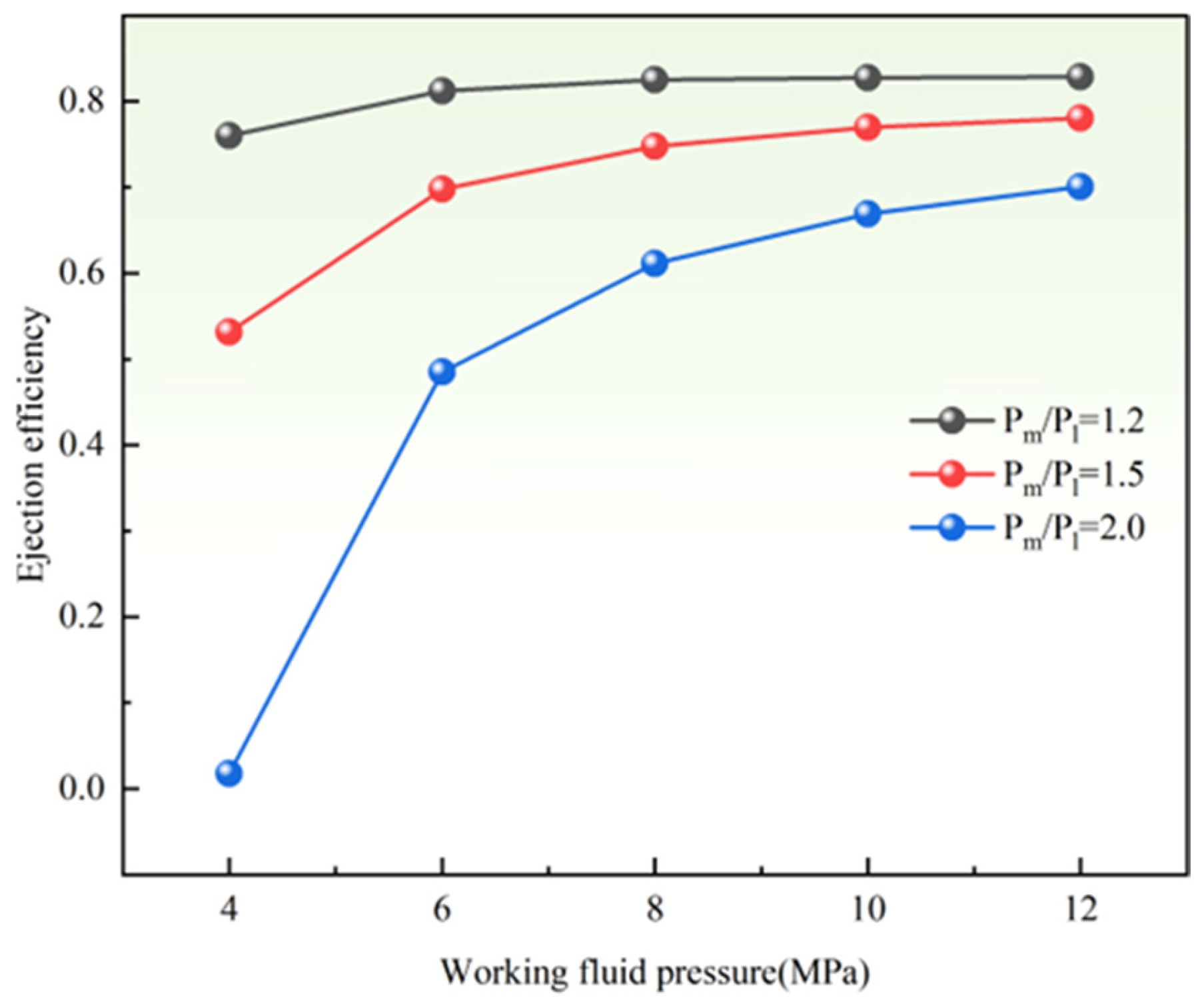
As shown in Figure 12, when the entrained fluid pressure is kept constant, the entrainment coefficient increases with the increase in working fluid pressure under different compression ratios. It is important to note that when the high-pressure value exceeds a certain threshold, the entrainment coefficient ceases to increase; excessively high working fluid pressure can lead to calculation non-convergence, i.e., a failure to correctly display simulation results. The maximum pressure shown in the figure is 12 MPa. During the simulation, poor convergence occurred at 14 MPa, and non-convergence emerged with further pressure increases. Therefore, to ensure data accuracy, the maximum working fluid pressure selected in this study was 12 MPa.

When the working fluid pressure is low, it cannot effectively entrain the entrained fluid, resulting in a small flow rate of the entrained fluid. Additionally, the low energy of the working fluid leads to insufficient mixing in the mixing chamber, resulting in low entrainment efficiency. As the working fluid pressure increases, its energy rises, carrying a larger flow rate of entrained fluid, promoting better mixing in the chamber, and enabling the mixed fluid to overcome backpressure more effectively, thus increasing entrainment efficiency. However, as the working fluid pressure continues to increase, its flow cross-section expands correspondingly. When the pressure reaches a critical value, the flow cross-section of the working fluid equals or even exceeds the longitudinal cross-section of the mixing chamber, causing the working fluid to completely occupy the chamber. This drastically reduces the flow rate of the entrained fluid, halting the improvement of entrainment efficiency and even leading to entrainment failure. Therefore, to ensure optimal ejector performance, the working fluid pressure should be reasonably set.

Notably, the positive correlation between working gas pressure and ejector efficiency in Figure 12 does not conflict with prior negative ejector coefficient observations. The key boundary condition disparity resides in entrained gas pressure: 1.6 MPa (Figure 12) versus 4 MPa (negative cases), yielding a lower outlet backpressure resistance for mixed gas under the same compression ratio. At elevated compression ratios, even the minimum working fluid pressure in Figure 12 transfers enough energy to enable flow discharge, explaining the efficiency increase with pressure. Conversely, negative efficiency arose when working gas energy failed to overcome backpressure at high compression ratios, causing flow reversal; increasing working gas pressure in such cases would alleviate backflow and raise efficiency.

3.2.3. Influence of Entrained Fluid Pressure on Entrainment Efficiency

With the working fluid pressure and outlet pressure kept constant, the variation in entrainment efficiency with changes in entrained fluid pressure was simulated by adjusting the entrained fluid pressure. The selected pressure values are listed in

Table 12. Selection of ejection fluid pressure.

Ejection Fluid Pressure/MPa	Working Fluid Pressure/MPa	Mixed Fluid Pressure/MPa
4	10	5/6/8
3.2		5/6/8
2.4		5/6/8
1.6		5/6/8
0.8		5/6/8

.

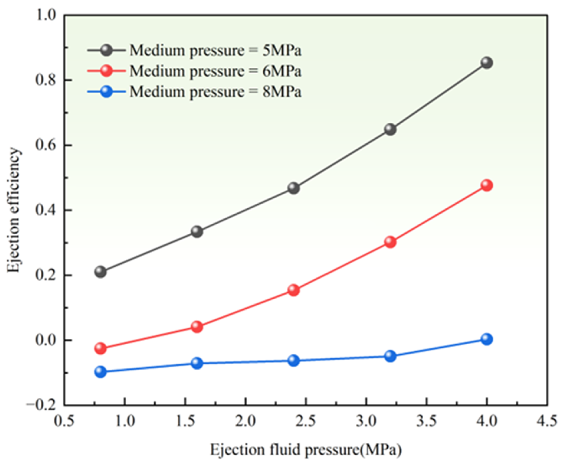
Figure 13 shows that when the working fluid pressure and outlet pressure are constant, the entrainment efficiency increases with the increase of entrained fluid pressure. However, when the outlet pressure is high and the entrained fluid pressure is low, the entrainment coefficient may become negative, which is caused by fluid backflow and the ejector’s failure to operate normally.

After the working fluid enters the nozzle from the inlet, it undergoes an acceleration and depressurization process. Before entering the mixing chamber, its pressure drops to a lower value (nozzle outlet pressure), and the entrained gas is entrained into the mixing chamber. When the entrained gas pressure is low, the pressure difference between it and the nozzle outlet pressure is small, resulting in insignificant entrainment of the entrained gas and insufficient driving force to enter the mixing chamber, leading to poor gas mixing. Meanwhile, due to the influence of high backpressure at the outlet, partial backflow of the entrained fluid occurs, resulting in low entrainment efficiency and negative entrainment coefficients. As the entrained gas pressure increases, the pressure difference with the nozzle outlet pressure expands, thereby enhancing the driving force for entrainment into the mixing chamber. Consequently, the mass flow rate of the entrained fluid increases, and the entrainment efficiency improves accordingly.

In summary, to ensure the ejector operates with optimal performance, its operating conditions must be reasonably configured to function under suitable operating conditions [34,35,36]. For the selection of compression ratio, a smaller value should be adopted as much as possible under working requirements to improve entrainment efficiency. The working fluid pressure should be appropriately chosen within a suitable range to balance entrainment efficiency and avoid resource waste. Under constant other conditions, higher entrained fluid pressure is recommended to enhance entrainment efficiency.

3.3. Network Case Validation

3.3.1. Solution of Pipeline Network Equations

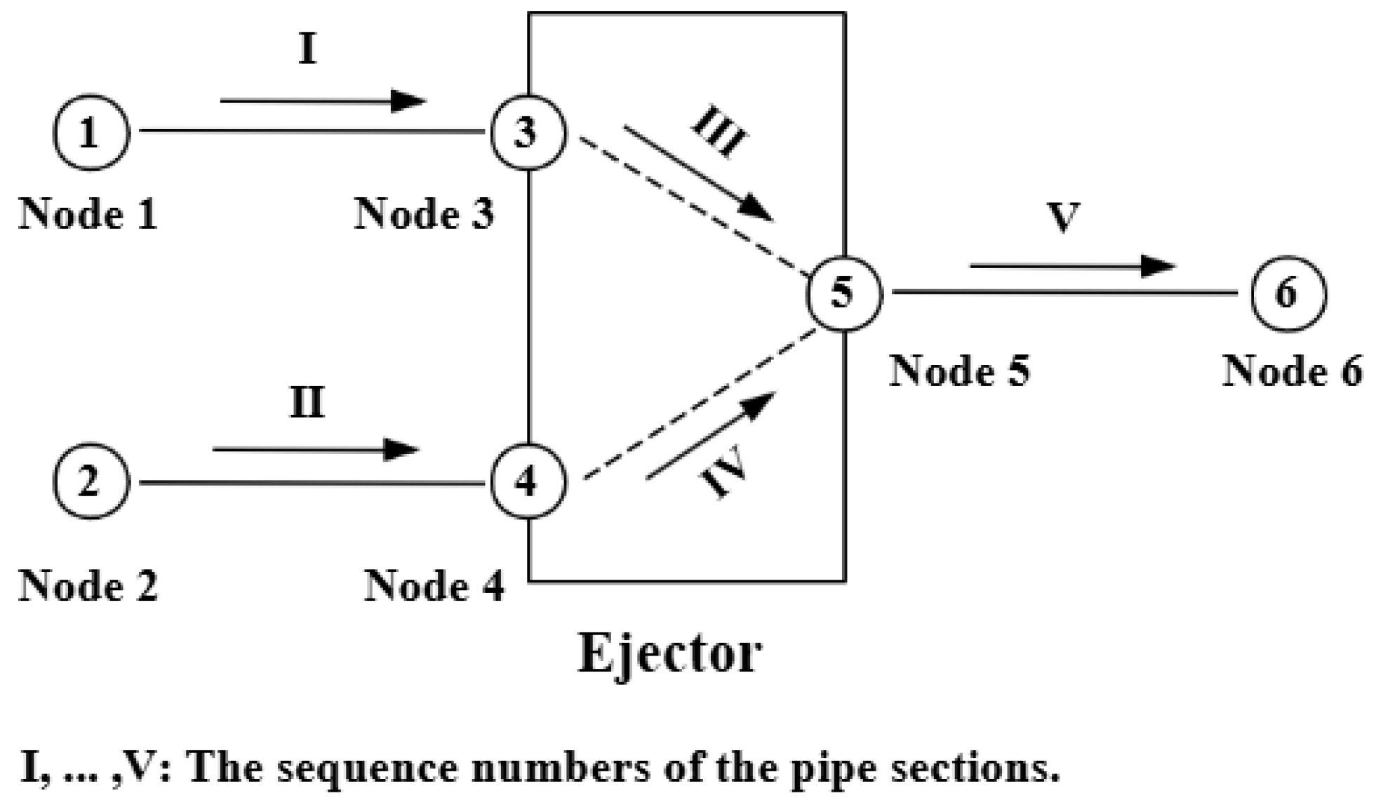
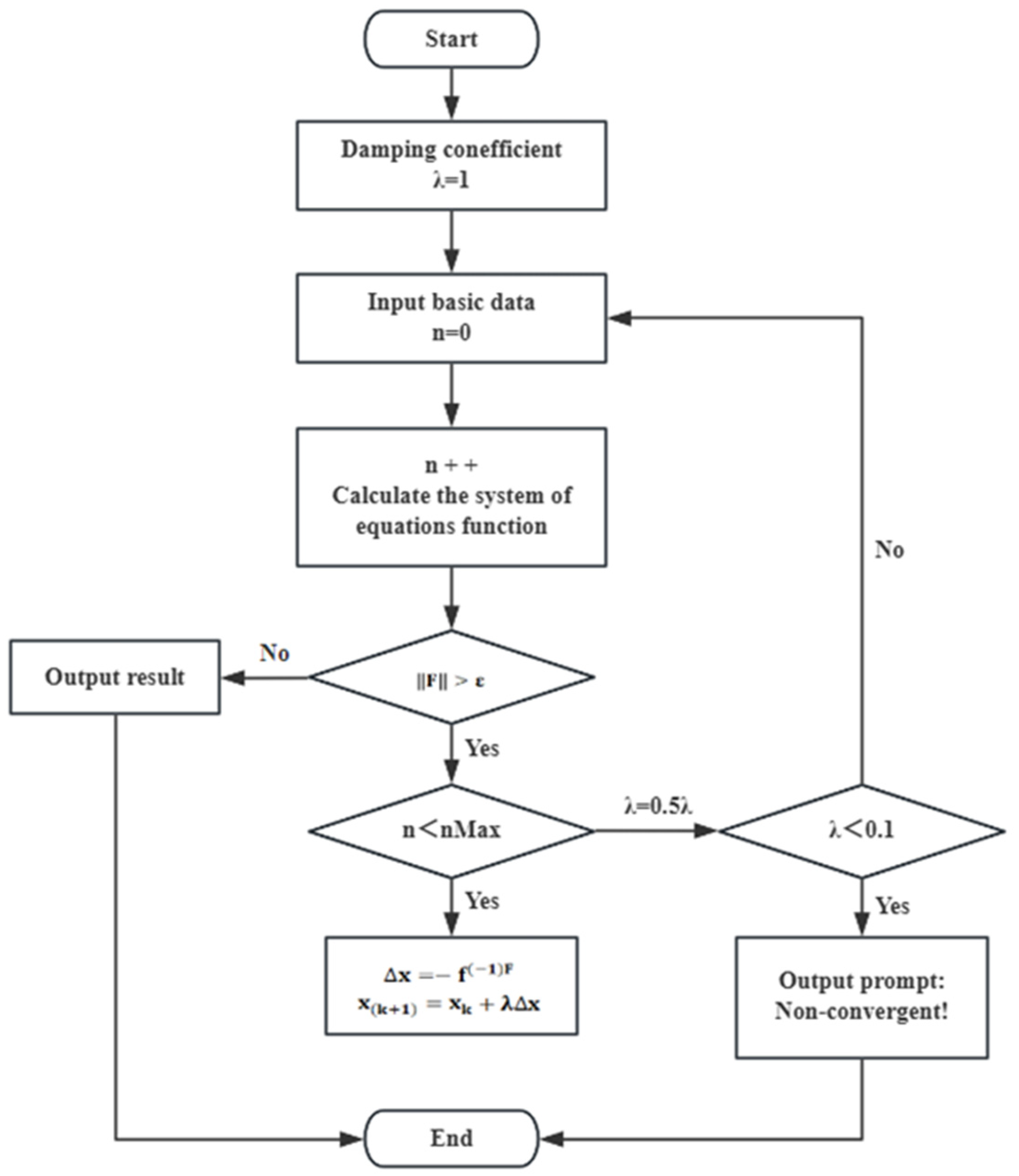
To verify the effectiveness of the designed ejector in a pipeline network, this study uses pipeline network calculation software for simulation validation. For pipeline network equations, the node method is generally employed, where the flow rate of a pipeline segment is expressed as a function of the pressures at both ends of the segment based on the segment’s flow formula. This eliminates the unknown parameter of segment flow rate Q, such that the number of unknowns in the calculation matches the number of equations (both equal to the specified number of pipeline segments). At this point, the unknown variables in the system of equations are only the nodal pressures and loads, enabling iterative calculation. However, if the ejector’s characteristic equation is to be added to the system, the high/low-pressure gas flow rates of the ejector cannot be directly expressed as functions of port pressures. Therefore, the system of equations must be simplified before solving. The simplified pipe network model is shown in Figure 14, and the calculation iteration method is shown in Figure 15.

3.3.2. Program Structure

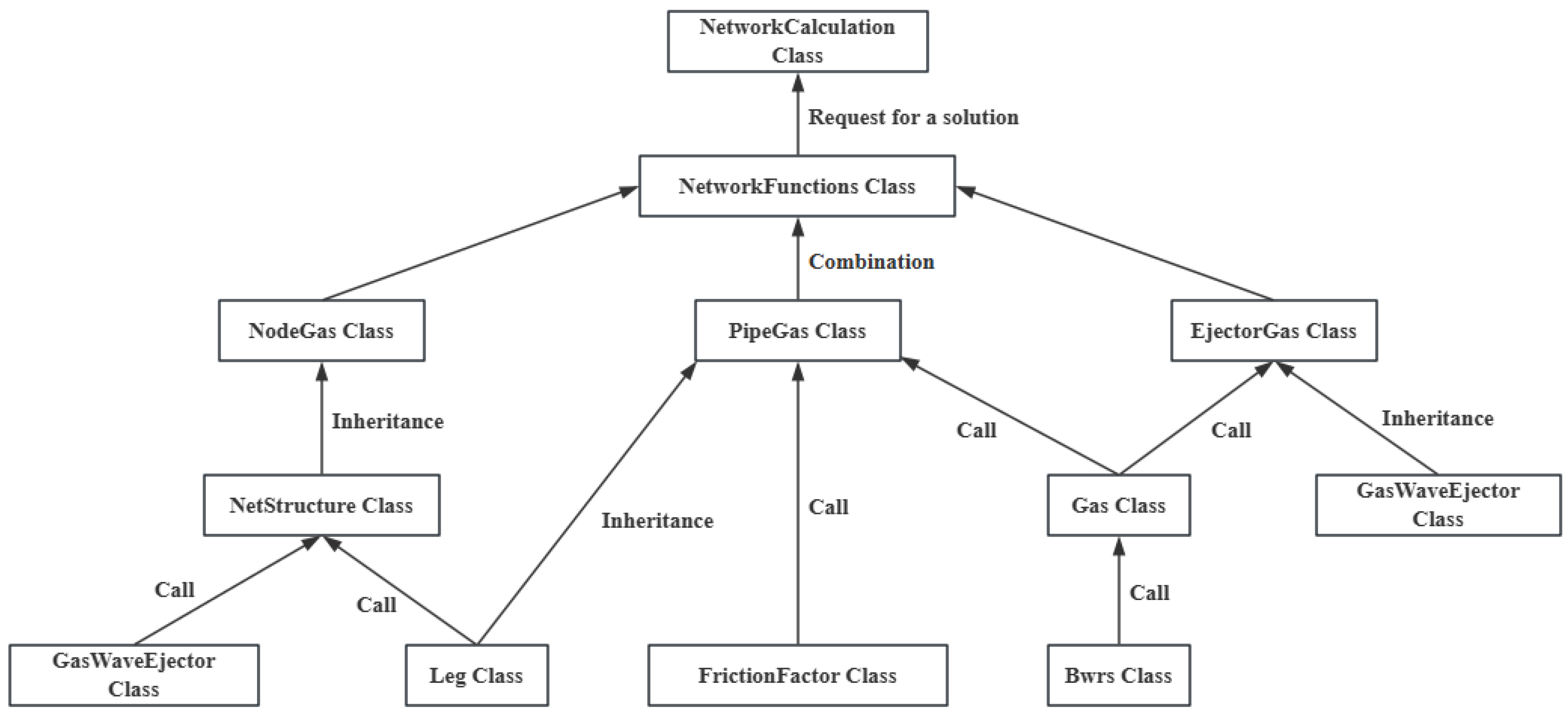
Drawing reference from the relevant research of Yu Li et al. [20], the solution process was coded into a computational program using Java 2024. The program primarily includes modules for natural gas physical property calculations, hydraulic friction coefficient calculations, gas pipeline segment modeling, pipeline network structure modeling, ejector modeling, and system of equations solving. Each component is implemented as a distinct class, and the program structure is illustrated in Figure 16.

3.3.3. Case Validation

Data from the Shenfu Gas Field were selected for case analysis, as shown in

Table 13. Data of Shenfu Gas Field.

Years	Tight Gas		Coalbed Methane
	Wellhead Pressure (MPa)	Average Daily Gas Production (m3/d)	Wellhead Pressure (MPa)	Average Daily Gas Production (m3/d)
0	15.16	5000.0	3.00	5000
1	9.46	5000.0	2.1	2310
2	5.64	5000.0	1.0	3300
3	2.03	5000.0	0.8	3300
4	1.96	3500.0	0.7	3300
5	1.86	3080.0	0.6	2826
6	1.74	2710.4	0.5	2420
7	1.61	2385.2	0.4	2073
8	1.46	2098.9	0.3	1775
9	1.30	1847.1	0.3	1520
10	1.14	1625.4	0.2	1302
11	0.97	1430.4	0.2	1115
12	0.79	1258.7	0.2	955
13	0.60	1107.7	0.2	818
14	0.42	974.8	0.2	700
15	0.25	857.8	0.2	600
16	0.12	754.8	0.2	514
17	0.06	663.6	0.2	440
18	0.06	566.7	0.2	377
19	0.05	415.2	0.2	323
20	0.05	333.3	0.2	276

.

For ease of calculation, the pipeline network structure selected as a case study in this paper consists of three pipelines and one ejector, with the general structure shown in Figure 17.

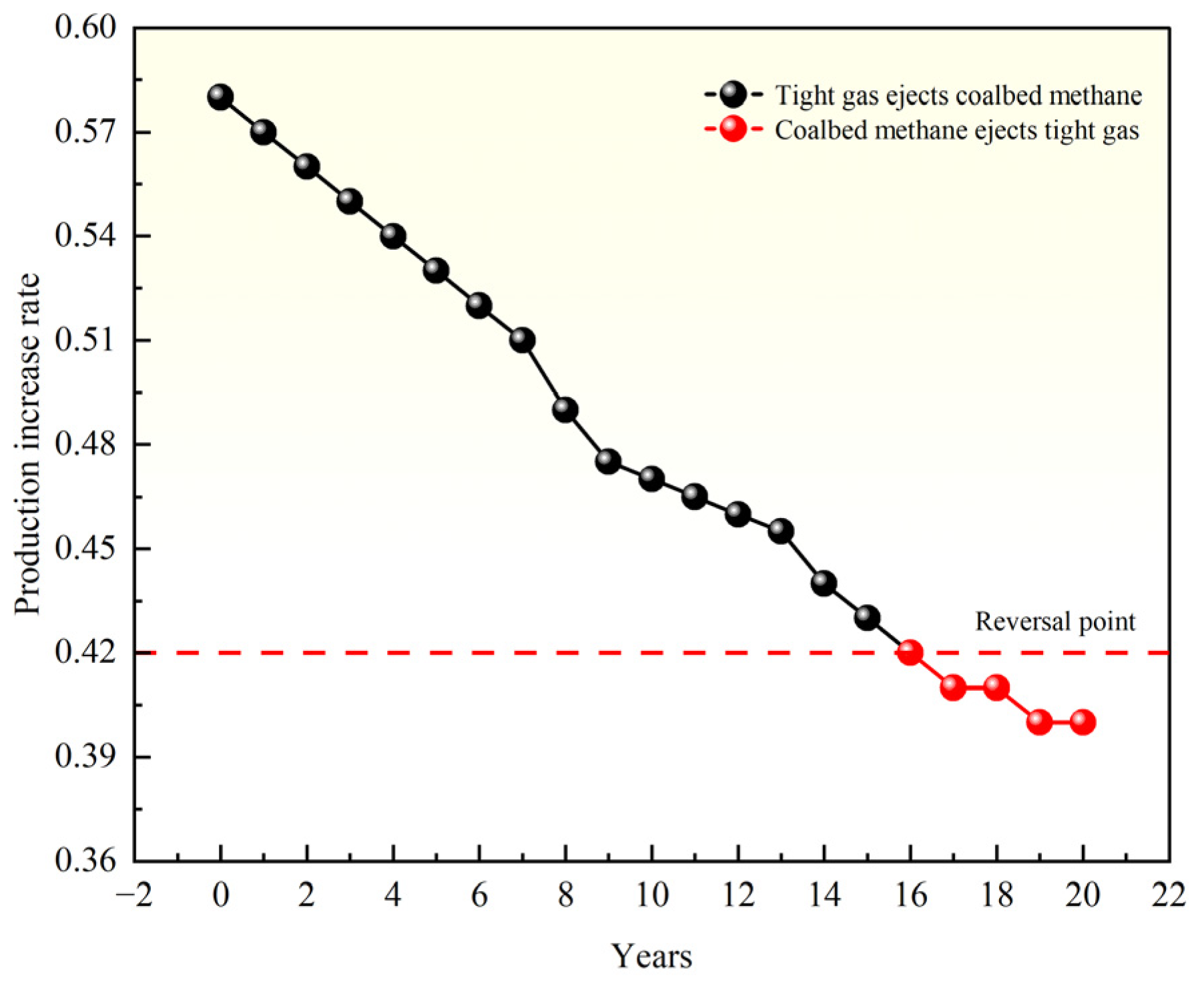
After inputting the parameters of each pipeline segment, gas properties, and ejector parameters, the solution can be performed, and the results are shown in Figure 18.

The curves indicate that the production enhancement effect of the ejector decreases over the years of exploitation. Since the pipeline network in this case consists of only a single high-pressure and a single low-pressure gas well, the calculated production enhancement rate theoretically represents the entrainment rate of a single ejector. In the sixteenth year, as the coalbed methane well pressure exceeded that of the tight gas well, the conditions were reversed in the calculation, with coalbed methane serving as the working fluid to entrain tight gas. The results demonstrate that the ejector model proposed in this paper can function normally in pipeline networks, though its effectiveness diminishes with prolonged production. Therefore, ejectors should be deployed in the early stages of production to maximize benefits. Specifically, deploying the ejector in the first production year of a gas well yields the maximum benefit, which gradually decreases with increasing production years until the pressure of the high-pressure gas well drops below the threshold to support normal ejector operation by the 16th year.

4. Discussion

In conclusion, this numerical study systematically explored the intricate influences of structural and operational factors on ejector efficiency, offering novel insights and practical guidance for the design and optimization of ejector systems in the field of oil and gas storage and transportation engineering.

Regarding structural parameters, the research reveals that each critical element, namely, the mixing chamber length L_m, diameter D_m, nozzle spacing L_c, and diffuser length L_d, exhibits a non-linear correlation with the entrainment coefficient, with optimal values varying according to the compression ratio. Specifically, when the pressure ratio P_m/P_l is 1.2, the most efficient configuration features L_m = 210 mm, D_m = 56 mm, L_c = 18 mm, and L_d = 715.03 mm; at P_m/P_l = 1.5, the optimal setup is L_m = 210 mm, D_m = 34 mm, L_c = 18 mm, and L_d = 475.72 mm; when P_m/P_l = 2.0, the best-performing parameters are L_m = 180 mm, D_m = 24 mm, L_c = 16 mm, and L_d = 315.69 mm. These findings underscore the necessity of considering the interplay between structural parameters and operating conditions during ejector design. Among these structural factors, D_m has the most pronounced impact on entrainment efficiency, while L_c has the least, indicating that adjusting D_m can serve as a key strategy for efficiency enhancement in practical applications.

As for operating conditions, an increase in the compression ratio results in elevated outlet pressure, causing a decline in entrainment efficiency. For instance, across all tested inlet pressure scenarios, adopting a lower compression ratio is more conducive to maintaining high-efficiency operation. The working fluid pressure positively affects the entrainment efficiency until reaching a critical point. Beyond this threshold, further increases bring marginal improvements and may even lead to operational instabilities, emphasizing the importance of precise pressure optimization to avoid resource waste. Meanwhile, under the condition of constant outlet pressure, augmenting the entrained fluid pressure can effectively enhance ejector efficiency. Therefore, it is recommended to utilize the highest feasible entrained fluid pressure within the operational range.

Notably, through pipeline network simulation software, this study validates the effectiveness of ejectors in improving gas production in real-world networks, filling a research gap compared with previous studies that primarily focused on standalone ejectors. However, the observed time-dependent performance degradation of ejectors highlights the significance of early deployment for maximizing economic benefits in engineering projects. According to the calculation results in Figure 18, deploying the ejector in the first production year of a gas well yields the maximum benefit, which gradually decreases with increasing production years until the pressure of the high-pressure gas well drops below the threshold to support normal ejector operation by the 16th year. Overall, the findings of this study provide valuable theoretical and practical references for optimizing ejector performance, which can be extended to enhance the efficiency and economic viability of oil and gas storage and transportation systems.

References

- Wang, Z.; Abu, D.; Feng, C.; Sun, F.; Ma, H. Structural Parameter Optimization and Work Performance Simulation of Surface Jet Ejectors. China Pet. Mach. 2024, 52, 124–131. [Google Scholar] [CrossRef]
- Kuś, T.; Madejski, P. Numerical Investigation of a Two-Phase Ejector Operation Taking into Account Steam Condensation with the Presence of CO2. Energies 2024, 17, 2236–2238. [Google Scholar] [CrossRef]
- Zhang, J.; Liu, Y.; Guo, Y.; Zhang, J.; Ma, S. Numerical Study on Flow and Noise Characteristics of High-Temperature and High-Pressure Steam Ejector. Energies 2023, 16, 4158. [Google Scholar] [CrossRef]
- Zheng, J.; Hou, Y.; Tian, Z.; Jiang, H.; Chen, W. Simulation Analysis of Ejector Optimization for High Mass Entrainment under the Influence of Multiple Structural Parameters. Energies 2022, 15, 7058. [Google Scholar] [CrossRef]
- Hong, B.; Li, X.; Li, Y.; Chen, S.; Tan, Y.; Fan, D.; Song, S.; Zhu, B.; Gong, J. An improved hydraulic model of gathering pipeline network integrating pressure-exchange ejector. Energy 2022, 260, 125101. [Google Scholar] [CrossRef]
- Zhang, X. Trial-production of Wellhead Jet Ejector Tools for Low-Pressure Gas Wells. Master’s Thesis, Southwest Petroleum University, Chengdu, China, 2014. [Google Scholar]
- Zhang, Z.; Ji, W.; Chen, Y.; Zeng, L.; Liu, Y.; Liu, F. Parameter Optimization Research of Static Ejectors Based on the Working Conditions of Natural Gas Wells in a Certain Area. Chem. Equip. Technol. 2024, 45, 35–40. Available online: https://link.cnki.net/doi/10.16759/j.cnki.issn.1007-7251.2024.08.008 (accessed on 6 July 2025).
- Chen, X.; Xiao, L.; Xu, J. Influence of Structural Parameters on the Two-Dimensional Flow Field in the Ejector. Therm. Power Gener. 2009, 38, 40–43+47. [Google Scholar] [CrossRef]
- Hou, Y.; Chen, F.; Zhang, S.; Chen, W.; Zheng, J.; Chong, D.; Yan, J. Numerical simulation study on the influence of primary nozzle deviation on the steam ejector performance. Int. J. Therm. Sci. 2022, 179, 107633. [Google Scholar] [CrossRef]
- Jin, X.; Xie, S.; Li, S.; Ren, L.; Wei, C.; Guan, Y. Research on the Influence of Operating Parameters on the Performance of Ejectors for Low-pressure Coalbed Methane Wells. Chin. J. Hydrodyn. (Ser. A) 2020, 35, 656–662. [Google Scholar] [CrossRef]
- Mei, S. Research on the Structure and Liquefaction Law of LNG Ejectors. Master’s Thesis, Huazhong University of Science and Technology, Wuhan, China, 2021. [Google Scholar] [CrossRef]
- Dong, J.; Hu, Q.; Yu, M.; Han, Z.; Cui, W.; Liang, D.; Ma, H.; Pan, X. Numerical investigation on the influence of mixing chamber length on steam ejector performance. Appl. Therm. Eng. 2020, 174, 115204. [Google Scholar] [CrossRef]
- Muzaber, A.; Bassmaji, N.; Kaddah, A. A new mixing chamber geometry design for supersonic ejector performance optimization using computational fluid dynamics. Int. J. Thermofluids 2025, 25, 101047. [Google Scholar] [CrossRef]
- Liu, H.; Hao, Q.; Zhang, Y.; Jin, C. Numerical Simulation Research on the Performance of a New-type Ejector with a Straight-pipe Section in the Working Nozzle. Cryog. Supercond. 2023, 51, 90–95. [Google Scholar] [CrossRef]
- Sokolov, E.Я.; Zingel, H.M. Ejectors; Huang, Q., Translator; Science Press: Beijing, China, 1977. [Google Scholar]
- Liu, P.; Wang, H.; Wu, J.; Zhu, L.; Hu, D. Optimal Design and Verification of Key Structural Parameters of Ejectors. J. Dalian Univ. Technol. 2017, 57, 29–36. [Google Scholar]
- Bartosiewicz, Y.; Aidoun, Z.; Mercadier, Y. Numerical assessment of ejector operation for refrigeration applications based on CFD. Appl. Therm. Eng. Des. Process. Equip. Econ. 2006, 26, 604–612. [Google Scholar] [CrossRef]
- Sun, Z. Research on Optimization of Wellhead Ejection Pressurization Tools for Shale Gas Wells. Master’s Thesis, China University of Geosciences (Beijing), Beijing, China, 2019. [Google Scholar] [CrossRef]
- Wang, Q. Numerical Simulation and Experimental Study on Transcritical CO2 Two-Phase Flow Ejectors. Master’s Thesis, Shandong University, Jinan, China, 2022. [Google Scholar] [CrossRef]
- Li, Y. Pipeline Network Calculation and Operation Optimization Based on Gas-Wave Ejectors. Master’s Thesis, China University of Petroleum (Beijing), Beijing, China, 2019. [Google Scholar] [CrossRef]
- Chen, H.; Chen, B.; Xu, Z.; Ge, J.; Chen, H.; Zhong, Z. A Thermodynamic Model for Performance Prediction of an Ejector with an Adjustable Nozzle Exit Position. Processes 2025, 13, 879. [Google Scholar] [CrossRef]
- Unterluggauer, J.; Buruzs, A.; Schieder, M.; Sulzgruber, V.; Lauermann, M.; Reichl, C. Design of Ejectors for High-Temperature Heat Pumps Using Numerical Simulations. Processes 2025, 13, 285. [Google Scholar] [CrossRef]
- Friso, D. Mathematical Modelling of the Entrainment Ratio of High Performance Supersonic Industrial Ejectors. Processes 2022, 10, 88. [Google Scholar] [CrossRef]
- Malakootikhah, M.; Valizadehderakhshan, M.; Shahbazi, A.; Mehrabani-Zeinabad, A. Developing a New Algorithm to Design Thermo-Vapor Compressors Using Dimensionless Parameters: A CFD Approach. Processes 2022, 10, 601. [Google Scholar] [CrossRef]
- Galindo, J.; Serrano, J.R.; Dolz, V.; Iljaszewicz, P. Impact of Mesh Resolution and Temperature Effects in Jet Ejector CFD Calculations. Appl. Sci. 2025, 15, 3880. [Google Scholar] [CrossRef]
- Ghorbani, B.; Zendehboudi, S.; Saady, N.M.C. Advancing Hybrid Cryogenic Natural Gas Systems: A Comprehensive Review of Processes and Performance Optimization. Energies 2025, 18, 1443. [Google Scholar] [CrossRef]
- Lysak, I.A.; Lysak, G.V.; Konyukhov, V.Y.; Stupina, A.A.; Gozbenko, V.E.; Yamshchikov, A.S. Efficiency Optimization of an Annular-Nozzle Air Ejector under the Influence of Structural and Operating Parameters. Mathematics 2023, 11, 3039. [Google Scholar] [CrossRef]
- Bukharin, N.; Hassan, E.M. Numerical and Experimental Investigation of Supersonic Binary Fluid Ejector Performance. Fluids 2023, 8, 197. [Google Scholar] [CrossRef]
- Bernat, M.; Nagy, S.; Smulski, R. Use of a New Gas Ejector for a TEG/TREG Natural Gas Dehydration System. Energies 2023, 16, 5011. [Google Scholar] [CrossRef]
- Zhao, Y.; Li, H.; Hu, D.; Liu, M.; Feng, Q. Study on the Performance of Collaborative Production Mode for Gas Wave Ejector. Sustainability 2022, 14, 7261. [Google Scholar] [CrossRef]
- Van den Berghe, J.; Dias, B.R.; Bartosiewicz, Y.; Mendez, M.A. A 1D model for the unsteady gas dynamics of ejectors. Energy 2023, 267, 126551. [Google Scholar] [CrossRef]
- Jing, H.; Yuan, Z.; Gao, J.; Chen, W.; Chong, D. Prediction of adjustable steam ejectors performance through Integration of numerical simulation and theoretical model. Appl. Therm. Eng. 2025, 267, 125841. [Google Scholar] [CrossRef]
- Li, H.; Wang, X.; Ning, J.; Zhang, P.; Huang, H.; Tu, J. Numerical investigation of the nozzle expansion state and its effect on the performance of the steam ejector based on ideal gas model. Appl. Therm. Eng. 2021, 199, 117509. [Google Scholar] [CrossRef]
- Li, C.; Li, Y. Investigation of entrainment behavior and characteristics of gas–liquid ejectors based on CFD simulation. Chem. Eng. Sci. 2011, 66, 405–416. [Google Scholar] [CrossRef]
- Li, W.; Han, Q.; Wang, C.; Zhang, H.; Jia, L.; Wang, L.; Sun, W.; Xue, H. Influence of geometric parameters on ejector acoustics and efficiency in ejector refrigeration system. Int. J. Refrig. 2025, 169, 429–443. [Google Scholar] [CrossRef]
- Śmierciew, K.; Gagan, J.; Butrymowicz, D. Application of numerical modelling for design and improvement of performance of gas ejector. Appl. Therm. Eng. 2018, 149, 85–93. [Google Scholar] [CrossRef]
Disclaimer/Publisher’s Note: The statements, opinions and data contained in all publications are solely those of the individual author(s) and contributor(s) and not of MDPI and/or the editor(s). MDPI and/or the editor(s) disclaim responsibility for any injury to people or property resulting from any ideas, methods, instructions or products referred to in the content. |
© 2025 by the authors. Licensee MDPI, Basel, Switzerland. This article is an open access article distributed under the terms and conditions of the Creative Commons Attribution (CC BY) license (https://creativecommons.org/licenses/by/4.0/).