1. Introduction
Under the background of “double carbon”, low-carbon and environmentally friendly renewable energy power generation represented by wind power and photovoltaic is gradually replacing traditional power generation represented by thermal power. By the end of 2024, China’s new energy power generation capacity will be about 140 GW, accounting for 43% of the country’s total installed power generation capacity [
1]. According to the National Energy Administration, the proportion will exceed 60% in 2030. However, the stochastic and intermittent characteristics of new energy generation lead to dramatic fluctuations in the net load (system load minus new energy generation) of the new type of power system, which is characterized by intraday fluctuations of more than 50%, increased frequency of fluctuations on a single day, and growth in the duration of fluctuation time, which makes the new type of power system’s ramping problem more and more serious, and the system’s demand for ramping capacity is increasingly serious. The system’s demand for ramping capacity is increasing [
2,
3].
To cope with this challenge, the international power market has constructed a diversified ramping product system: the flexible ramping product (FRP, Flexible Ramping Product) of California independent system operator (CAISO) [
4], the ramping capability product (RCP, Ramping Capability Product) of Midcontinent Independent System Operator (MISO) [
5], and the ramping capability product (RCP, Ramping Capability Product) of Southwest Power Pool (SPO). Midcontinent Independent System Operator (MISO)’s Ramping Capability Product (RCP, Ramping Capability Product), Southwest Power Pool (SPP)’s Ramping Product (RP) of Southwest Power Pool (SPP) in the United States [
6], the Fast Reserve (FR) product of National Grid ESO (NG ESO) in the United Kingdom [
7], and Germany’s reliance on the 15 min ramp capacity auction mechanism in the intraday market to balance net load fluctuations [
8]. In China, ramping is explicitly included in the new auxiliary service varieties at the policy level [
9], and the Shandong power market will take the lead in carrying out the pilot operation of ramping auxiliary service market in 2023, marking a key step towards the fine regulation of China’s power market mechanism [
10].
In recent years, the gradual maturation of artificial intelligence technology has been widely applied in the field of prediction. The literature [
11] uses the N-HiTS deep learning model to predict the previous day’s market electricity prices, combined with mixed-integer linear programming (MILP) to optimize the charging and discharging strategies of retired electric vehicle batteries, thereby maximizing benefits and resource recycling. Reference [
12] proposed a load frequency control method based on safe reinforcement learning, integrating energy storage systems through a constrained Markov decision process (CMDP) framework, and using an LSTM cost prediction network and the original dual deep deterministic policy gradient (PD-DDPG) algorithm to achieve rapid frequency regulation under safety constraints, significantly improving the system’s dynamic performance. In the field of uphill demand forecasting, the existing research results deconstruct the hill-climbing demand into two dimensions: deterministic demand and uncertain demand [
13]. Deterministic hill-climbing demand originates from net load time series fluctuations, which can be predicted with high accuracy by mature algorithms such as ARIMA [
14], SVM [
15], LSTM [
16], deep learning [
17,
18], and hybrid methods [
19,
20]; whereas, uncertain hill-climbing demand is affected by the coupled effects of multiple factors, such as load prediction error, new energy output prediction error, and so forth, and the CAISO in the existing study The histogram statistics method adopted by CAISO simplifies the forecast error to a fixed distribution, resulting in the loss of intraday dynamic features and overly conservative demand estimation; the traditional regression model has limited ability to capture dynamic features such as net load ramping rate and duration; probabilistic methods such as quantile regression, although capable of constructing forecast intervals, suffer from the defects of difficult to take into account the coverage of the intervals and the economy. In the field of probabilistic forecasting, wind/photovoltaic power forecasting and short-term load forecasting have formed a relatively mature methodology system, such as dynamic interval estimation based on multivariate quantile regression [
21], conditional probability modeling with Bayesian networks [
22,
23], and nonparametric distribution fitting with kernel density estimation [
24], etc. These data-driven techniques provide important references for determining the boundary of net load forecasting errors. However, the formation mechanism of net load prediction error has significant particularity. First, its uncertainty source presents the nonlinear superposition characteristics of wind and light load prediction errors, and the error distribution presents a multi-peak pattern; second, the prediction error dynamically correlates time-varying characteristics such as the net load climbing rate and the fluctuation duration, and the static assumptions of the traditional probabilistic model mechanistically conflict with the dynamic characteristics of the net load, so it is difficult to meet the new power system climbing rate and the fluctuation duration directly with the existing analysis methods. Therefore, it is difficult to directly use the existing analysis method to meet the demand for fine-grained assessment of the climbing capacity of the new type of power system.
Based on the above analysis, for the problem of uncertain creeping demand forecasting, this paper constructs a CNN-LSTM hybrid neural network to achieve a breakthrough in uncertain creeping demand forecasting through the synergistic extraction of spatio-temporal features and dynamic probabilistic modeling. The model locally senses the correlation of wind and light load prediction errors with the convolutional layer of CNN, captures the morphological features of error multi-peak distribution (e.g., the double-peak superposition formed by PV midday power dips and wind power nighttime fluctuations) with the multi-scale convolutional kernel, and at the same time resolves the temporal dependence between the net load ramping rate, the fluctuation phases, and durations through the gating loop unit of LSTM, which solves the problem of dynamic feature extraction and dynamic probability modeling in the traditional approach due to the loss of dynamic features caused by the static distribution assumption of the traditional method being solved.
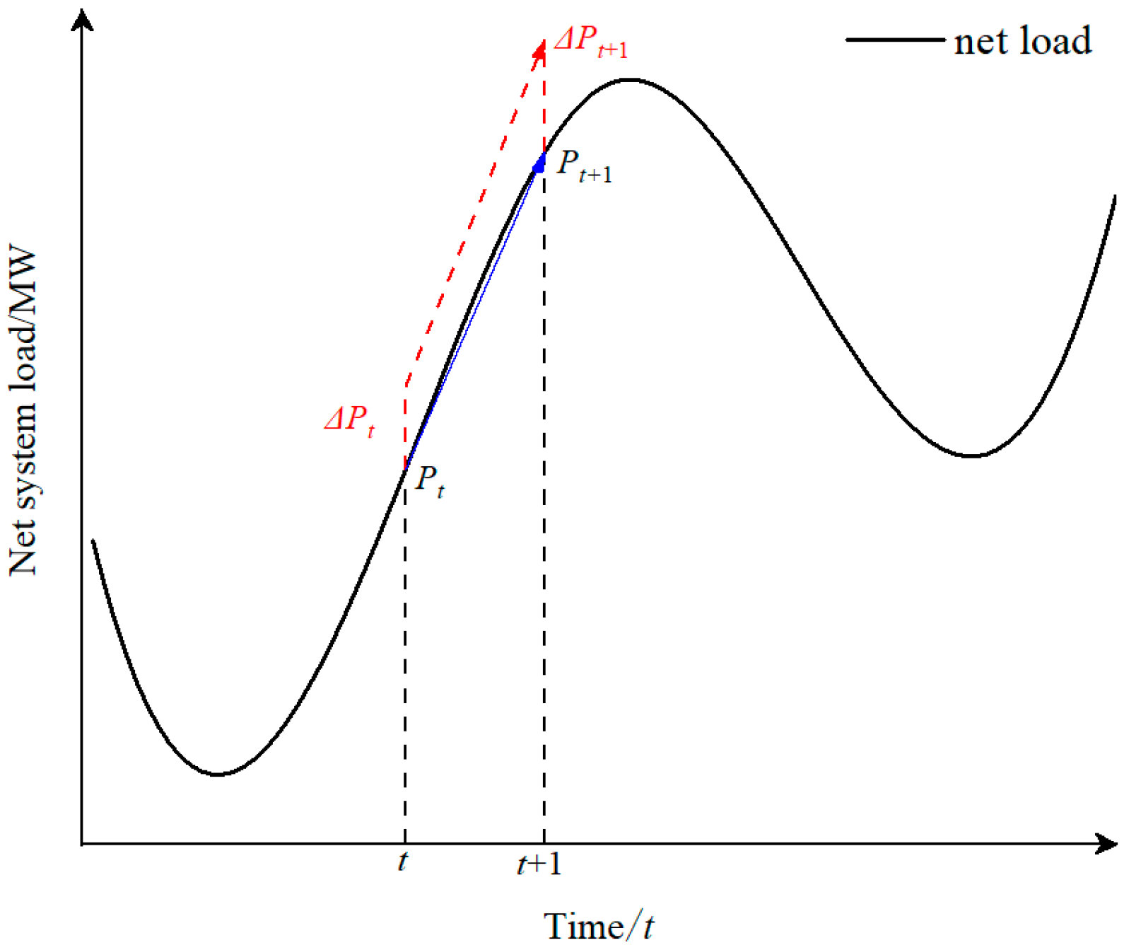
2. Climbing Demand Modeling
The creeping demand in the new power system arises from the time-series fluctuation of net load on the one hand and from the net load forecast error on the other hand, as shown in
Figure 1.
From
Figure 1, it can be seen that the climbing demand of the system should be portrayed in terms of both climbing capacity and climbing rate, as shown in Equation (1).
where
is the climbing capacity demand of the system,
is the deterministic climbing capacity demand calculated from the net load forecast value,
is the uncertain climbing capacity demand caused by the net load forecast error,
and
are the net load forecast values at time
and time
, respectively,
and
are the net load forecast errors at time
and time
, respectively, and s is the rate of climbing.
The climbing demand type of the system at any moment is unidirectional, i.e., up and down climbing demand types. As shown in Equation (1), the climbing type of the system at moment
depends on the relationship between the magnitude of deterministic climbing demand and uncertain climbing demand, and the statistics of the relationship between the relative relationship of
,
and the type of the system’s climbing demand are shown in
Table 1.
At present, the capacity and type of deterministic creepage demand can be obtained directly from the net load forecast value, but the capacity and type of uncertainty creepage demand are closely related to the forecast accuracy; if the uncertainty creepage demand forecast accuracy is high, the uncertainty creepage demand is small, and the overall creepage demand of the system depends on the deterministic creepage demand, which can be determined directly; if the uncertainty creepage demand forecast accuracy is low, the forecast error range is larger, and the type and capacity of the overall system’s climbing demand is difficult to determine, so improving the uncertainty climbing demand prediction accuracy is key to solving the system’s total climbing demand refinement assessment.
3. Multi-Source Coupled Feature-Driven CNN-LSTM Interval Prediction Modeling
3.1. Net Load Forecast Error Analysis
Uncertainty in ramping demand mainly stems from the forecasting errors of load and new energy output, and the causes of forecasting errors are characterized by significant multi-sourcing and coupling. This study shows that the load prediction error is related to multi-dimensional factors such as customer’s behavioral pattern, day type (weekday/holiday), season, temperature, etc., while the new energy output prediction error is affected by the synergistic effect of meteorological conditions (wind speed, light intensity) and seasonal cycle. Moreover, the influencing factors do not act independently, but through complex coupling mechanisms (e.g., temperature-usage behavior correlation, wind speed–light intensity dynamic compensation), which makes it difficult for traditional unidimensional modeling methods to effectively capture such nonlinear spatio-temporal correlations.
To this end, this study proposes a CNN-LSTM-based net load forecast error modelling method. The core advantage of the CNN-LSTM hybrid architecture lies in its ability to synergistically analyze multi-dimensional dynamic coupling mechanisms and multi-scale temporal evolution characteristics. To address cross-dimensional nonlinear interaction features in net load prediction errors, such as temperature–electricity consumption behavior and wind speed–light intensity, a multi-channel convolutional neural network (CNN) is employed to extract local correlations in the feature space (e.g., synergistic effects of meteorological elements), overcoming the limitation of models like GRU/Transformer in adequately capturing non-temporal spatial patterns. Additionally, to capture long-term and short-term dependencies such as intraday fluctuations and seasonal trends (e.g., sudden changes in load during holidays), a bidirectional LSTM gating mechanism is employed to model temporal dynamic evolution, addressing the issue of long-term information decay caused by the simplified structure of GRU. Compared with the Transformer’s reliance on massive data and the limitations of TCN in handling non-stationary time series, this architecture adaptively fuses the local coupling features of CNN and the long-short-term dependency features of LSTM through a dynamic attention mechanism, and constructs a quantile regression model to quantify the prediction error of non-Gaussian distributions, ultimately achieving an optimized balance in spatio-temporal cascaded modeling. In scenarios involving high-dimensional spatio-temporal feature interactions (e.g., strong coupling of multiple variables such as wind and solar load), this architecture demonstrates significant improvements over traditional methods. For example, SVM struggles to handle high-dimensional feature interactions, RF is insufficient for modeling continuous temporal dynamics, and BPNN cannot decouple coupled effects due to its single-structure design. CNN-LSTM provides a technical foundation that balances prediction accuracy and robustness for the precise assessment of uncertain ramping demands through the adaptive extraction of spatio-temporal joint features.
3.2. Model Fundamentals
3.2.1. Principles of CNN Modeling
Extracting the correlation relationship between various factors such as wind speed, light intensity, temperature, and customer’s electricity behavior to establish a prediction model for net load prediction error is of great significance for the fine-grained assessment of uncertainty creeping demand. Convolutional neural network (CNN) is a deep learning model designed for processing spatially structured data (e.g., time-series signals, gridded weather data), and its core structure contains a convolutional layer, an activation function, and a pooling layer. The convolutional layer performs local weighted summation on the input data through a sliding window, extracts local correlation features (e.g., wind speed, light intensity, historical static load error) between multi-dimensional influences (e.g., wind–scenery complementary effect, nonlinear relationship between light and load), and significantly reduces the number of model parameters through parameter sharing; the activation function (e.g., ReLU) introduces nonlinearities to enhance the model’s ability to express complex interactions; the pooling layer introduces nonlinearities through the pooling function, and enhances the model’s ability to express complex interactions. Regarding expression capability, the pooling layer retains key features through downsampling, which empowers the model to be robust to changes in data location. For the task of net load prediction error, the CNN can stack multi-layer convolutional modules to abstract higher order correlations (e.g., the dynamic effect of combined wind and light on the error) layer by layer from the input multi-dimensional time-series data (e.g., the channel composed of wind speed–light-historical error). By automatically mining the internal and external correlations of non-independent factors such as wind–scenery load (e.g., the coupling relationship between sudden changes in light intensity and load error during local time periods), CNN can effectively capture the nonlinear spatio-temporal dependence between multiple factors, thus improving the accuracy of the prediction of net load prediction error.
Each convolutional layer in CNN can be represented by Equation (2):
where
is the input vector of the convolutional layer;
is the output vector of the convolutional layer with the position of the ith row and the jth column;
is the activation function (e.g., Sigmoid, Leaky, ReLU, etc.);
is the weight matrix of the convolutional kernel connected to the kth feature map;
is the bias vector of the feature map; and * denotes the convolution operation.
The pooling layer is a key dimensionality reduction and feature enhancement module in convolutional neural networks (CNNs), and is mainly used to reduce the feature dimensionality, thus reducing the amount of computation and the number of parameters and mitigating the risk of overfitting. The feature extraction requirement of this study focuses on the multi-source coupling characteristics of prediction error causes, so the max pooling method (Max Pooling) is used for the selection of pooling strategy. By extracting the maximum activation value within the local receptive field, this algorithm can effectively capture the key features with significant differentiation in the error propagation process, while weakening the interference of secondary noise on the feature representation. This pooling mechanism with feature selection provides high information density input features for the subsequent LSTM network analysis of the temporal correlation of multi-dimensional errors. Compared with the smoothing property of average pooling, max pooling retains feature saliency and avoids the dilution effect of global averaging that may produce key information.
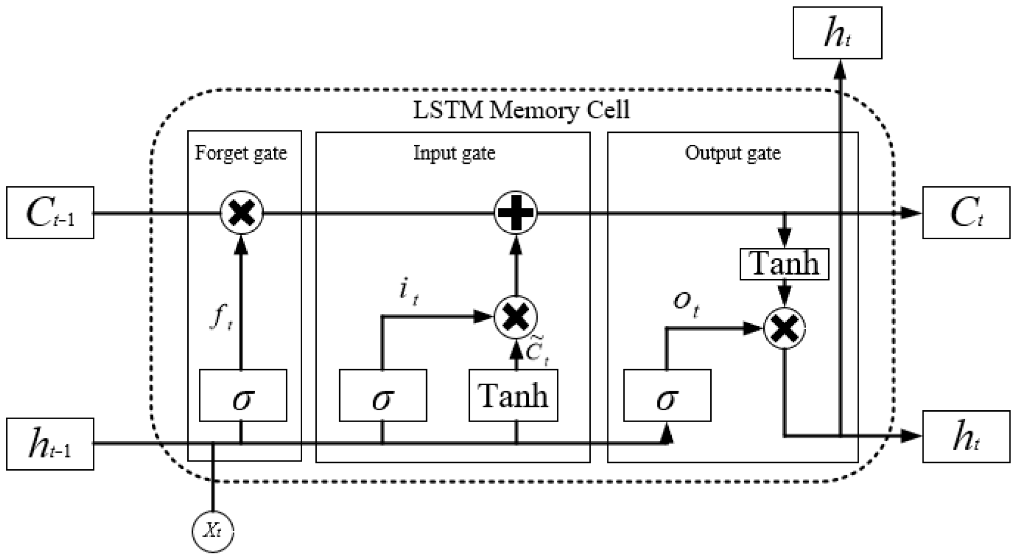
3.2.2. Principles of LSTM Modeling
LSTM (long short-term memory network) is an efficient model proposed to solve the problem of gradient vanishing or explosion faced by traditional recurrent neural networks (RNNs) in long sequence training, and its core innovation lies in the introduction of cell state and the dynamic regulation mechanism consisting of three gating units (forgetting gate, input gate, and output gate) (as shown in
Figure 2).
Forget gate (Forget Gate) is the core mechanism for controlling the retention and discarding of historical information in LSTM; it works by dynamically evaluating the correlation between the historical memory and the current input and deciding which redundant or invalid information to remove from the previous cell state, thus freeing up the storage space for the new important information, and avoiding the degradation of the model’s performance caused by information overload, and is calculated as shown in Equation (3).
where
is the weight of the forgetting gate, which controls the forgetting strength of the old memories;
is the weight matrix of the forgetting gate;
is the hidden state of the previous moment;
is the input of the current time step;
is the bias term of the forgetting gate; and
represents the Sigmoid activation function.
Input gate is the core mechanism for controlling the integration of new information and memory update in LSTM; its role is to filter and integrate valuable new features into the cellular state (long-term memory) by dynamically evaluating the importance of the current inputs, and, at the same time, collaborate with the forgetting gate to complete the logic of “forgetting before learning” to ensure that the model continues to optimize the knowledge base in complex time-series tasks. The input gate consists of two key computational processes to ensure that the model continues to optimize the knowledge base during complex temporal tasks.
- (1)
The input gate weights are calculated to determine which information in the current input contributes to long-term memory, as shown in Equation (4).
where
is the input gate weight, which controls the learning intensity of the candidate memories;
is the weight matrix of the input gate;
is the bias term of the input gate.
- (2)
Candidate memories for the current input are generated to determine new features that potentially need to be learned, as shown in Equation (5).
where
is the candidate memory;
is the weight matrix of the candidate memory;
is the bias term of the candidate memory;
denotes the hyperbolic tangent activation function.
Using the results of the input gate weight calculation and the generated candidate memories, the information fusion of historical and new knowledge can be performed to update the long-term memory of the cell state, as shown in Equation (6).
Output gate (Output Gate) is the core mechanism in LSTM for controlling the external visibility of memory information, and its role is to decide what should be delivered or output to the next layer at the current moment by dynamically screening the valid information in the cellular state (long-term memory), as shown in Equation (7).
where
is the output gate weight, which controls the visibility of the cell state
;
is the current hidden state, which is passed to the next moment as short-term memory or used for prediction;
is the weight matrix of the output gate;
is the bias term of the output gate;
denotes the Sigmoid activation function; and
denotes the Hyperbolic Tangent activation function.
3.3. CNN-LSTM Interval Prediction Model Introducing Quartile Regression Method
The core advantage of interval prediction of net load prediction error over point prediction is to quantify the uncertainty caused by the superposition of new energy output prediction error and load prediction error, and, by outputting prediction intervals at different confidence levels (e.g., 90%), not only can it provide dynamic risk boundaries for grid scheduling but it can also provide guidance for the allocation of spare capacity to enhance the economic operation level of the power system.
Traditional CNN-LSTM models use mean square error (MSE) or mean absolute error (MAE) as the loss function, and the output is the point forecast value. The model proposed in this paper takes wind speed, light intensity, net load prediction value, electricity consumption behavior, and other influencing factors as inputs, extracts the potential features among the influencing factors through the convolution and pooling operation of the CNN layer, and takes the extracted features as inputs to the LSTM layer. The three gates and the memory unit unique to the LSTM layer can further screen the features extracted by the CNN, so that important features are retained through the memory unit, unimportant features are retained through the memory unit, and unimportant features are discarded by the forgetting gate. The quantile regression (QR) method is introduced, and the quantile loss function (Quantile Loss) is used to replace the loss function of the traditional CNN-LSTM, so that the model output results are changed from a single point prediction output to the prediction results of multiple quantiles. According to the theory of quantile regression, the median (50% quantile) prediction result itself can be used as a robust estimation of the point prediction, and the loss function corresponding to each quantile is the quantile loss function during training, while the loss function of the median is actually the mean absolute error (MAE). Therefore, under the quantile regression framework, the median prediction value can be used as a point prediction result, and the prediction results of other different quantiles can be used to construct the prediction intervals at different confidence levels, realizing the point prediction and interval prediction of the net load prediction error.
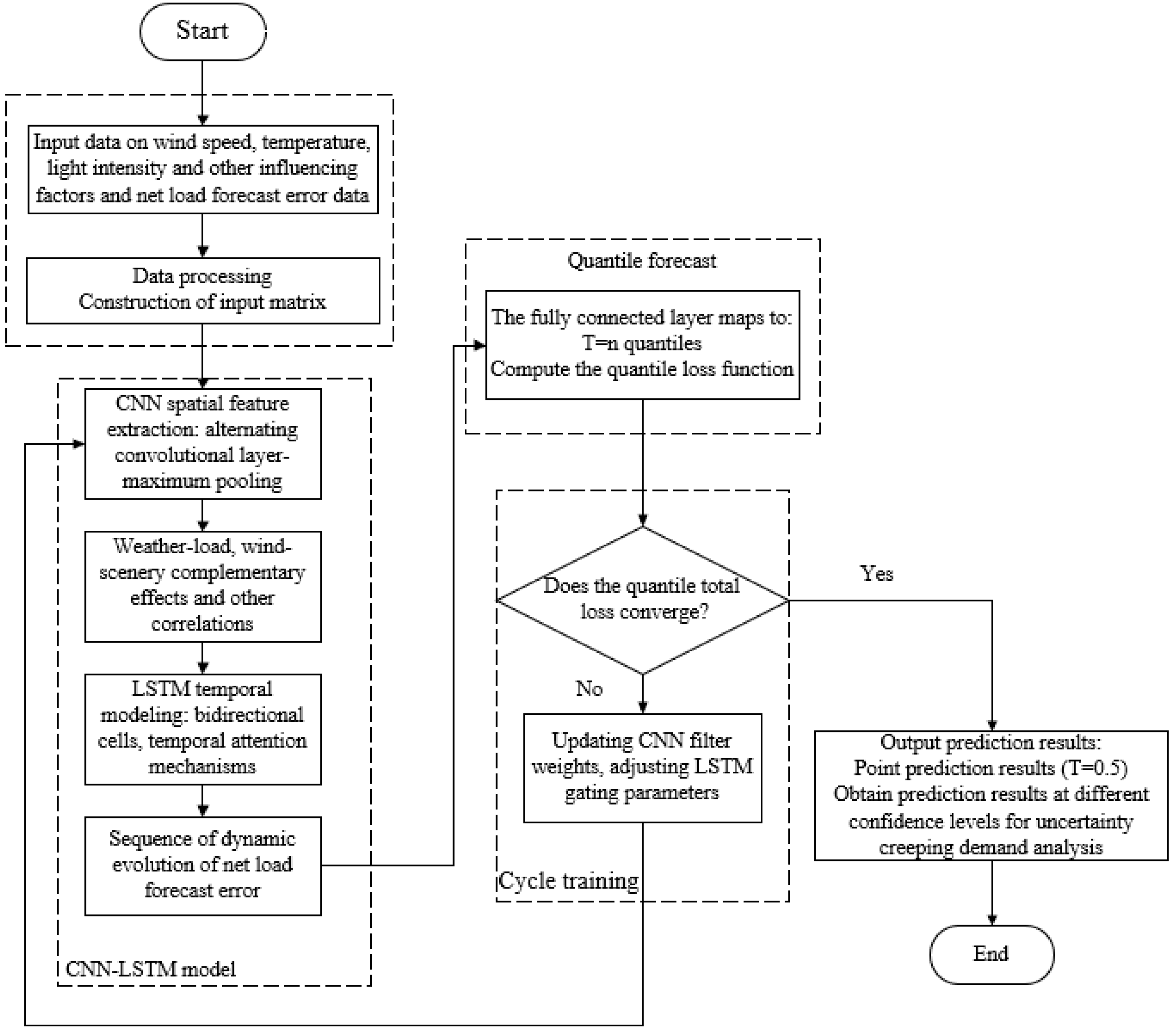
In this paper, we propose the CNN-LSTM (CNN-LSTM-QR) model that introduces the quantile regression method for point prediction and interval prediction process of net load prediction error, as shown in
Figure 3.
Step 1: Input data such as wind speed, light intensity, temperature, and electricity behavior with historical net load prediction error data, and perform data preprocessing to construct an input matrix.
Step 2: The input matrix is subjected to CNN feature extraction to obtain the coupling relationship between the influencing factors and is used as the input to the LSTM layer, which performs time-series modeling to obtain the dynamic evolution sequence of the net load prediction error and inputs the results into the quantile prediction module.
Step 3: The fully connected layer maps features to T = n quantiles, quantifying prediction intervals at different confidence levels. The quantile loss function is calculated to measure the degree of deviation of the predicted value from the true value at high and low confidence intervals.
Step 4: Calculate the total loss of the model and determine whether the loss converges. If it converges, terminate the training, output the prediction results of different quartiles, construct the point prediction value (T = 0.5) and the results of prediction intervals at different confidence levels, and calculate the uncertainty creeping demand at different confidence levels. If it does not converge (loss fluctuation > threshold), then update the model parameters and cycle the training model until it converges.
4. Example Analysis
The relevant data required for this paper are selected from the actual operation data and forecast data of a provincial power grid from 1 January to 31 December 2020, including load, wind speed, light intensity, temperature, wind power output, and photovoltaic output data, etc., with a time interval of 15 min, totaling 35,040 sets of data, and the dataset is divided into a training set and a test set according to 7:3. Based on the above raw data, the net load actual value and forecast value are obtained, and further data such as net load forecast error are generated, which are used as the basic data for example analysis. For missing and outlier values in the dataset, if the neighboring data points are all normal, the mean method is used to calculate and fill in the missing values; if the data adjacent to the point are all missing or outliers, the piecewise cubic Hermite interpolation method is used for interpolation. The dataset is normalized before being input into the model. To prevent model gradient explosion, the dataset with 15 min intervals from the previous 7 days is used as the model input for prediction, and the load data with 15 min intervals from the next day is used for prediction.
The input layer of the model uses 7 days of historical time-series samples, covering load, wind speed, light intensity, temperature, wind power, and photovoltaic output data, to capture the periodic patterns of multi-source features. The model first passes through a CNN module containing 64 convolutional kernels with a size of 3 × 3, using ReLU as the activation function, followed by a 2 × 2 pooling layer to extract local spatial features of intraday fluctuations.
The model first passes through a CNN module, which includes 64 3 × 3 convolution kernels with a ReLU activation function, followed by a 2 × 2 pooling layer to extract local spatial features of intraday fluctuations. The data then pass through a two-layer LSTM structure, with the first layer retaining sequence states using 128 neurons and the second layer extracting temporal dependencies using 64 neurons, both employing the tanh activation function to model long-term correlations. The final output is a daily scale prediction result generated by a fully connected layer with 96 neurons (linear activation). To optimize generalization capability, a triple dropout mechanism is introduced during training—0.2 after the CNN output, 0.3 between LSTM layers, and 0.2 before the fully connected layer—to suppress overfitting. An early stopping criterion is used to control the maximum number of training epochs to 100, and the Adam optimizer is employed for parameter tuning. The batch size is set to 32 to balance memory efficiency and gradient stability. Input data undergo normalization preprocessing to eliminate dimensional differences.
The forecasting strategy is implemented using a rolling structure, employing a daily rolling strategy. Specifically, during the forecasting process, data from the preceding 7 consecutive days (i.e., 672 data points) at 15 min intervals are used as model input to forecast the subsequent 1 day (i.e., 96 data points) of load data. During the entire test set evaluation phase, this input window moves forward along the timeline on a daily basis. Each time, the latest historical data are used to predict the subsequent full day’s data, after which the window shifts forward by one day. This achieves rolling predictions that cover the entire test period. The final prediction results and accuracy are based on this rolling prediction strategy across the entire test set.
4.1. Selection of Evaluation Indicators
In order to evaluate the quality of point prediction and interval prediction results, root mean square error (RMSE), mean absolute percentage error (MAPE), and coefficient of determination R2 are selected as evaluation indicators for point prediction results, and mean interval width (MIW) and prediction interval coverage probability (PICP) are selected as evaluation indicators for interval prediction results in this paper.
- (1)
Root mean square error (RMSE) is used to measure the magnitude of the average absolute deviation of the predicted value from the actual value, reflecting the level of absolute error in the prediction, as shown in Equation (8).
where
is the actual value of the net load forecast error,
is the predicted value of the net load forecast error, and
n is the number of samples.
- (2)
Mean absolute percentage error (MAPE) is used to assess the average percentage deviation of the prediction error relative to the actual value, which visualizes the relative accuracy of the prediction, as shown in Equation (9).
- (3)
The coefficient of determination is used to quantify the model’s ability to explain the trend of load fluctuations, with higher values indicating that the model is better able to capture the intrinsic pattern of load changes rather than random noise, as shown in Equation (10).
where
is the average of the actual values of the net load forecast error.
- (4)
Average interval width (AIW) is used to quantify the average width of the prediction interval, reflecting the range of uncertainty in the prediction, as shown in Equation (11).
where
is the upper bound of the prediction interval for the
sample and
is the lower bound of the prediction interval for the
sample.
- (5)
Prediction interval coverage probability (PICP) is used to assess the probability that the true value falls within the prediction interval, reflecting the reliability of the interval; the higher the coverage, the stronger the reliability of the interval prediction, as shown in Equation (12).
where
is the actual value of the
net load prediction error,
is the indicator function, which takes 1 when the true value is within the interval and 0 otherwise.
4.2. CNN-LSTM-QR Model Prediction Performance Evaluation
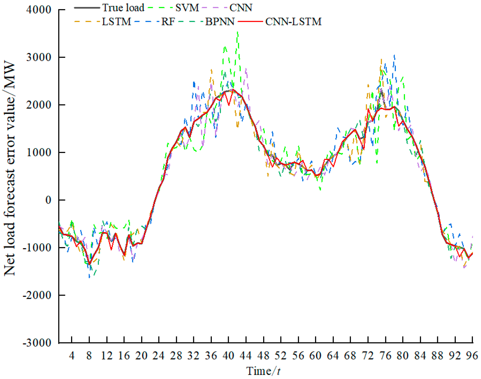
4.2.1. Point Prediction Performance Evaluation
In order to verify the scientificity and reliability of the model, this paper constructs a variable set containing each of the above factors, and predicts them using support vector machine (SVM), random forest (RF), backpropagation neural network (BPNN), convolutional neural network (CNN), LSTM model, and the model proposed in this paper, respectively, and the prediction results are shown in
Figure 4.
As shown in
Figure 4, both traditional models (SVM, RF, BPNN) and single deep learning models (CNN, LSTM) show significant deviations in the 0~20, 28~80, and 88~96 time periods, where the net load prediction error fluctuates drastically. SVM amplifies the error due to the insufficient fitting of the linear kernel function to the abrupt signals (e.g., steep fluctuations in the 88~96 time periods); RF in 28~80 has a pseudo-correlation error in the continuous fluctuation phase from 28 to 80 due to the discrete partitioning of the decision tree; BPNN is limited by the gradient vanishing problem, which makes it difficult to capture the high-frequency oscillations in the time period of 0~20; CNN lacks temporal modeling capability, which leads to the loss of dynamic correlation in the long time period of fluctuation from 28~80; and LSTM has a lag in the response to the sudden changes in the 88~96 time period, although it has the temporal memory property. In contrast, the model proposed in this paper extracts local mutation features (e.g., spikes in the 0~20 time period) through the convolutional layer, and captures inter-temporal dependencies (e.g., sustained oscillations in the 28~80 time period) through the LSTM layer, which is a collaborative spatio-temporal feature mining mechanism that effectively improves the robustness of the model in complex fluctuation scenarios.
In order to quantitatively compare the prediction effect of each model, the root mean square error (RMSE), the mean absolute percentage error (MAPE), and the coefficient of determination
R2 of the prediction results of different models are calculated, as shown in
Table 2. From the evaluation indexes in
Table 2, it can be seen that the prediction performance of traditional models (SVM, RF) is weak (MAPE:14.80–17.60%,
R2 ≤ 0.9302), and LSTM performs the best among deep learning models (MAPE: 9.53%,
R2 = 0.9654). The quantile CNN-LSTM model proposed in this paper achieves a significant breakthrough, with MAPE (3.20%) reduced by 66.4% and RMSE (91.48 MW) reduced by 56.6% compared with LSTM, and
R2 of 0.9934 approaching the theoretical limit value, which proves the effectiveness of the spatio-temporal feature fusion and quantile regression mechanism in improving prediction accuracy and robustness.
4.2.2. Evaluation of Interval Prediction Performance
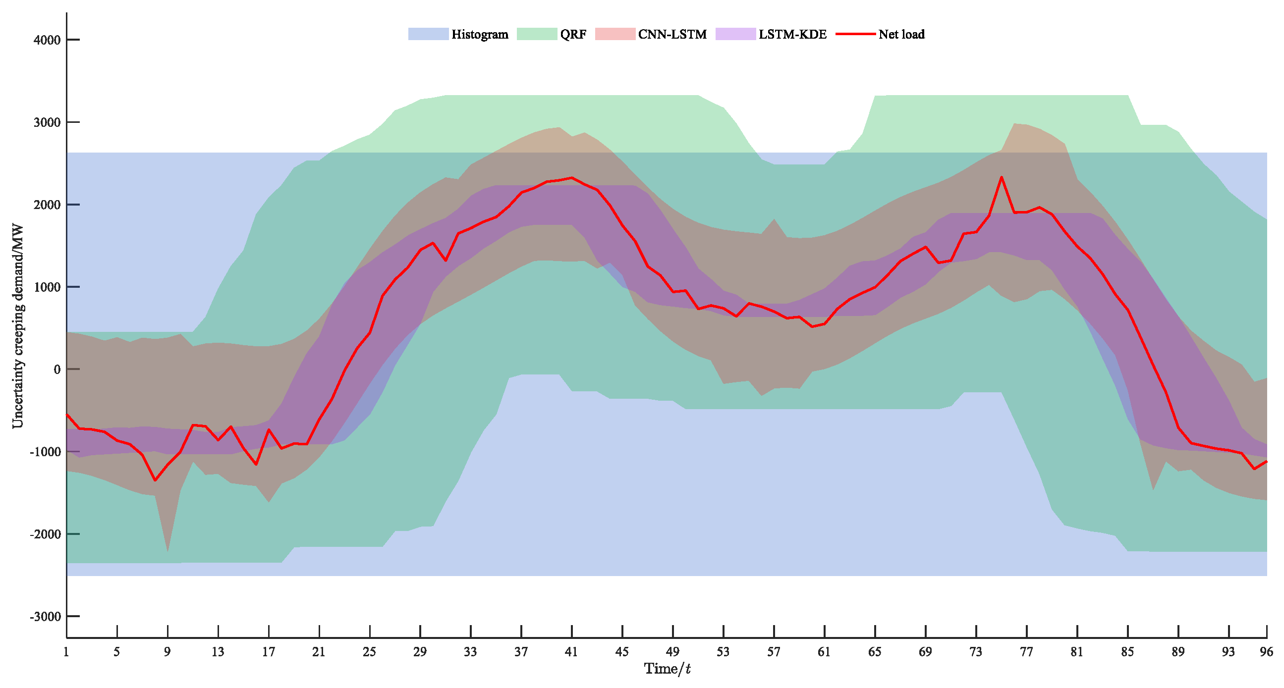
In order to verify the performance of CNN-LSTM-QR model uncertainty climbing demand prediction, this paper selects the statistical histogram method, which is actually applied in the CAISO climbing market, the quartile random forest model (QRF) commonly used in probabilistic prediction, and the LSTM kernel density estimation model (LSTM-KED) with the method of this paper for comparison of the prediction results with the results under the 95% confidence interval, which is selected to compare. As shown in
Figure 5, the average interval width (AIW) and prediction interval coverage probability (PICP) of the prediction results obtained from different prediction methods are calculated, and the results are shown in
Table 3.
A comparative analysis combining
Figure 5 and
Table 3 leads to the following conclusions.
For the prediction interval coverage PICP, the statistical histogram, quantile random forest model (QRF), and CNN-LSTM can reach 100% coverage, but the coverage of LSTM-KED is less than 100%, which is mainly due to the sensitivity of kernel density estimation to the assumptions of data distribution and the model’s insufficient capture of dynamic uncertainty. The statistical histogram obtains demand intervals from the histogram of net load forecast error data frequency, and its forecast result is fixed in one day, which cannot reflect the time-varying characteristics of the actual forecast error, and the forecast result is much higher than the actual demand, which easily causes a redundancy of resources if it is used as the basis for allocating and regulating the resources. QRF and CNN-LSTM models can both reflect the dynamic change of uncertainty in the demand of the climb, but the model with CNN-LSTM is less than 100%. Both QRF and CNN-LSTM models can respond to the dynamic change of uncertain climbing demand, but, compared with the CNN-LSTM model, the prediction result of the QRF model is too conservative, which easily causes resource waste.
The average interval width represents the uncertainty intensity, which can also indicate the size of the uncertainty creeping capacity demand required to guarantee the safe and stable operation of the power system, and the smaller the average interval width is under the premise of guaranteeing 100% coverage, it indicates that the model prediction results are more secure and economical. As can be seen from
Table 3, the average interval width of the CNN-LSTM model is 1992.90 MW, which is 38.8% of that of the traditional histogram method (5135.21 MW) and 50.31% of that of QRF (3960.75 MW), and the result proves that the CNN-LSTM model is able to capture the intrinsic laws among the influencing factors more efficiently by fusing the spatio-temporal features The results demonstrate that the CNN-LSTM model can more efficiently capture the intrinsic patterns among the influencing factors by fusing the spatial and temporal features, thus covering the real values with narrower intervals, and solving the problem of “over-conservatism” in the prediction results of traditional models.
4.2.3. Uncertainty Creep Needs Assessment
The interval prediction results at a given confidence level can be used to calculate the uncertainty creeping demand size, and the boundaries of the interval prediction results can represent the range of maximum/small maximum fluctuations of the actual values, then the average up/down creeping demand, as shown in
Table 4.
From the analysis in
Table 4, it can be seen that the CNN-LSTM method used in this paper performs optimally in the average hill-climbing demand prediction. Specifically, the average uphill climb demand of CNN-LSTM is 970.48 MW, which is 47.9% of the histogram method and 56.0% of the QRF; its average downhill climb demand is even more significantly reduced to 722.42 MW, which is 76.8% and 62.7% less than that of the histogram and QRF, respectively. This breakthrough in prediction performance stems from the dual advantages of the CNN-LSTM architecture; the convolutional neural network (CNN) is able to deeply mine the spatial correlation features of multi-source influencing factors, while the long-short-term memory network (LSTM) can accurately capture the dynamic evolution patterns in the time series. The synergy of the two significantly improves the ability to model the probability distribution of the net load forecast error, thus realizing the refined prediction of uncertain creeping demand, and providing more reliable technical support for the flexible resource dispatch of the power system.
5. Conclusions
In this paper, we study and analyze the uncertainty creeping demand caused by net load forecasting errors in a new type of power system, and we make the following contributions:
- (1)
The computational model of total system creeping demand is constructed, the effects of deterministic creeping demand and uncertain creeping demand on total creeping demand are analyzed, and the uncertain creeping demand forecasting model with multiple influencing factors as inputs is established.
- (2)
In this paper, we construct a dual prediction framework for uncertainty climbing demand by fusing the quantile regression method with a CNN-LSTM deep network, and realize the synergistic optimization of point prediction with high accuracy and interval prediction with reliability. The results show that the model proposed in this paper outperforms traditional models (SVM, RF, BPNN) and single deep learning models (CNN, LSTM) in point prediction results with higher prediction accuracy, which verifies the effectiveness of the spatio-temporal feature extraction module. In terms of interval prediction quality, when the confidence level is set to 95%, compared with the histogram and QRF benchmark models, the model in this paper maintains 100% interval coverage, while the average width of the predicted intervals is 38.8% and 50.31% of the two models mentioned above, the average upward climb demand is reduced by 52.1% and 44%, and the average downward climb demand is reduced by 76.8% and 62.7%, demonstrating a better balance of predicted economy and safety. This prediction method, which takes into account probabilistic boundary control and core trend capture, can provide a double guarantee for the fine-grained assessment of uncertainty creeping demand in new power systems, and has significant engineering application value. Subsequent studies will explore the dynamic quantile adjustment mechanism to enhance the adaptability of extreme scenarios.
The daily rolling strategy adopted in this paper improves computational efficiency. Model training takes 0.5–1 h, and after model training, predicting 96 data points per day takes only seconds, which meets the real-time application requirements of the power grid. However, the low-frequency update mechanism has some drawbacks, mainly manifested as follows:
- (1)
Real-time dynamic response is weakened, and the 24 h update cycle and 15 min sampling frequency are seriously mismatched. If sudden disturbances occur during the forecast period (such as severe convective weather or a sharp drop in photovoltaic output), they cannot be dynamically fed back to the input window, significantly weakening the model’s ability to adapt to intraday fluctuations.
- (2)
Long-term characteristics are fragmented, and fixed-length historical windows (such as 7 days) interrupt the continuity of meteorological evolution (such as cross-week cold wave events), which may lead to the systematic loss of key process information during window sliding.
The above-mentioned defects may give rise to risks such as deviations in the configuration of reserve capacity for daily scheduling and insufficient real-time control margins in a grid environment with high penetration of new energy sources.
To address the limitations of the daily rolling strategy, future research could design an event-triggered hybrid rolling mechanism that balances efficiency and timeliness through dynamic step length switching (e.g., enabling short-cycle updates on high-volatility days). A real-time feature injection architecture could be constructed to integrate short-term weather forecast data streams within the forecast period, enhancing the system’s ability to respond to sudden disturbances. Additionally, an intelligent historical window based on attention mechanisms could be developed to dynamically expand the historical coverage range based on feature importance (e.g., automatically extending to 14 days to capture cross-week weather events).
Author Contributions
Conceptualization, P.Y. and Z.C.; methodology, D.C. and H.Z. (Hao Zhang); validation, H.Z. (Hao Zhang), R.Y., and H.Z. (Hang Zhou); formal analysis, H.Z. (Hao Zhang); investigation, R.Y. and H.Z. (Hang Zhou); data curation, H.Z. (Hao Zhang); writing—original draft preparation, H.Z. (Hao Zhang), Y.Z.; writing—review and editing, D.C.; visualization, P.Y. and Z.C.; supervision, P.Y. and Z.C.; project administration, P.Y.; funding acquisition, P.Y. All authors have read and agreed to the published version of the manuscript.
Funding
This research is funded by the State Grid Liaoning Electric Power Co., Ltd. Jinzhou Power Supply Company, Contract No. SGLNJZ00HLJS2402984.
Data Availability Statement
The original contributions presented in this study are included in the article. Further inquiries can be directed to the corresponding author.
Acknowledgments
We would like to express our sincere gratitude to the reviewers for their professional opinions and valuable suggestions, and our heartfelt thanks to the editorial board of the journal for their efficient work in supporting the rigorous presentation of the scholarly results. We would like to pay tribute to the academic community.
Conflicts of Interest
Authors Peng Yu, Zhuang Cai, Dai Cui were employed by the company State Grid Liaoning Power Control Center. Author Hang Zhou was employed by the company Jinzhou Power Supply Company of State Grid Liaoning Electric Power Co., Ltd. The remaining authors declare that the research was conducted in the absence of any commercial or financial relationships that could be construed as a potential conflict of interest. The company had no role in the design of the study; in the collection, analyses, or interpretation of data; in the writing of the manuscript, or in the decision to publish the results.
Abbreviations
The following abbreviations are used in this manuscript:
| CAISO | California Independent System Operator |
| FRP | Flexible Ramping Product |
| MISO | Midcontinent Independent System Operator |
| RCP | Ramping Capability Product |
| SPP | Southwest Power Pool |
| RP | Ramp Product |
| NG ESO | National Grid ESO |
| FR | Fast Reserve |
| ARIMA | Autoregressive Integrated Moving Average |
| SVM | Support Vector Machine |
| LSTM | Long Short-Term Memory |
| CNN | Convolutional Neural Network |
| RF | Random Forest |
| BPNN | Back Propagation Neural Network |
| QR | Quantile Regression |
| MAE | Mean Absolute Error |
| RMSE | Root Mean Square Error |
| MAPE | Mean Absolute Percentage Error |
| MIW | Mean Interval Width |
| PICP | Prediction Interval Coverage Probability |
| QRF | Quantile Random Forest |
| KDE | Kernel Density Estimation |
References
- Zhou, D. By the end of 2024, China’s installed capacity of new energy power generation will account for more than 40%. China Foreign Energy 2024, 29, 59. [Google Scholar]
- Qiu, Y.; Lu, S.; Lu, H.; Luo, E.; Gu, W.; Zhuang, W. Flexibility of Integrated Energy Systems: Basic Connotations, Mathematical Model and Research Framework. Autom. Electr. Power Syst. 2022, 46, 16–43. [Google Scholar]
- Chen, Q.; Wu, M.; Liu, Y.; Wang, Y.; Xie, M.; Liu, M. Joint operation mechanism of spot electric energy and auxiliary service for windpower market-oriented Joint operation mechanism of spot electric energy and auxiliary service for windpower market-oriented accommodation. Electr. Power Autom. Equip. 2021, 41, 179–188. (In Chinese) [Google Scholar]
- CAISO. Flexible Ramping Product: Revised Draft Final Proposal; CAISO: Folsom, CA, USA, 2015. [Google Scholar]
- MISO. Ramp Capability for Load Following in MISO Markets White Paper; MISO: Carmel, IN, USA, 2016. [Google Scholar]
- Electricity Market and Dispatch Operation in the United States; China Electric Power Press: Beijing, China, 2002.
- British National Grid. Demand Turn Up 2018 Interactive Guidance Document; National Grid ESO: London, UK, 2018. [Google Scholar]
- EPEX spot. Flexibility Is the Answer: European Power Exchange as a Component of Security of Supply During the Solar Eclipse; EPEX: Paris, France, 2015. [Google Scholar]
- National Energy Administration. Measures for the Management of Electricity Ancillary Services; National Energy Administration: Beijing, China, 2021. [Google Scholar]
- National Energy Administration Shandong Supervision Office. Notice on Issuing the “Trial Rules for the Trading of Shandong Power Ramping Ancillary Services Market”. Available online: https://sdb.nea.gov.cn/dtyw/tzgg/202402/t20240208_245961.html (accessed on 8 February 2024). (In Chinese)
- Kırat, O.; Çiçek, A.; Yerlikaya, T. A New Artificial Intelligence-Based System for Optimal Electricity Arbitrage of a Second-Life Battery Station in Day-Ahead Markets. Appl. Sci. 2024, 14, 10032. [Google Scholar] [CrossRef]
- Gao, S.; Li, Y.; Chen, X.; Liang, Z.; Liu, E.; Liu, K.; Zhang, M. Load Frequency Control of Power Systems with an Energy Storage System Based on Safety Reinforcement Learning. Processes 2025, 13, 1897. [Google Scholar] [CrossRef]
- Hu, Z.; Liu, J.; Zhang, K.; Liu, C.; Chen, L. Analysis of the demand-price curve mechanism in the U.S. hill-climbing ancillary services market. Electr. Demand Side Manag. 2024, 26, 113–118. [Google Scholar]
- Fang, N.; Chen, H.; Deng, X.; Xiao, W. Short-term power load forecasting based on VMD-ARIMA-DBN. J. Power Syst. Autom. 2023, 35, 59–65. [Google Scholar]
- Du, T.; Yang, Y.; Dong, S. Exploration of grid power load forecasting model based on support vector machine and intelligent algorithm. Petrochem. Technol. 2024, 31, 208–210. [Google Scholar]
- Wang, J.; Yu, J.; Kong, X. Medium- and long-term load forecasting model based on dual decomposition and bidirectional long and short-term memory networks. Grid Technol. 2024, 48, 3418–3426. [Google Scholar]
- Han, F.; Wang, X.; Qiao, J.; Shi, M.; Pu, T. A review of new power system load forecasting research based on artificial intelligence technology. Chin. J. Electr. Eng. 2023, 43, 8569–8592. [Google Scholar]
- Ma, H.; Yuan, A.; Wang, B.; Yang, C.; Dong, X.; Chen, L. A review and outlook of load forecasting research based on deep learning. High Volt. Technol. 2025, 51, 1233–1250. [Google Scholar]
- Jiao, J.J.; Liu, T.Y. Short-term load forecasting based on ICEEMDAN-IWOA-BiLSTM hybrid algorithm model. Electr. Autom. 2024, 46, 36–39. [Google Scholar]
- Liu, J.; From, L.; Xia, Y.; Pang, G.; Zhao, H.; Han, Z. Short-term power load forecasting based on combined DBO-VMD and IWOA-BILSTM neural network model. Power Syst. Prot. Control. 2024, 52, 123–133. [Google Scholar]
- Bracale, A.; Caramia, P.; De Falco, P.; Hong, T. Multivariate quantile regression for short-term probabilistic load forecasting. IEEE Trans. Power Syst. 2020, 35, 628–638. [Google Scholar] [CrossRef]
- Guo, M.; Kou, P.; Tian, R.; Zhang, Y.; Liang, D. Probabilistic wind speed prediction of multiple turbines within a wind farm based on Bayesian graph convolutional neural network. J. Electrotechnol. 2024, 1–16. [Google Scholar]
- Liu, X.; Pu, X.; Li, J.; Zhang, Z. Short-term wind power prediction by VMD-GRU based on Bayesian optimization. Power Syst. Prot. Control. 2023, 51, 158–165. [Google Scholar]
- Wang, S.; Sun, Y.; Hou, D.; Zhou, Y.; Zhang, W. Ultra-short-term adaptive probabilistic prediction of wind power based on multi-window wide kernel density estimation. High Volt. Technol. 2024, 50, 3070–3079. [Google Scholar]
| Disclaimer/Publisher’s Note: The statements, opinions and data contained in all publications are solely those of the individual author(s) and contributor(s) and not of MDPI and/or the editor(s). MDPI and/or the editor(s) disclaim responsibility for any injury to people or property resulting from any ideas, methods, instructions or products referred to in the content. |
© 2025 by the authors. Licensee MDPI, Basel, Switzerland. This article is an open access article distributed under the terms and conditions of the Creative Commons Attribution (CC BY) license (https://creativecommons.org/licenses/by/4.0/).


