Article

Critical Threshold for Fluid Flow Transition from Linear to Nonlinear in Self-Affine Rough-Surfaced Rock Fractures: Effects of Shear and Confinement

1
Key Laboratory of Xinjiang Coal Resource Green Mining, Ministry of Education, Xinjiang Institute of Engineering, Urumqi 830023, China
2
College of Mining Engineering and Geology, Xinjiang Institute of Engineering, Urumqi 830091, China
3
State Key Laboratory of Intelligent Construction and Healthy Operation and Maintenance of Deep Earth Engineering, China University of Mining and Technology, Xuzhou 221116, China
4
State Key Laboratory of Coal Mine Disaster Dynamics and Control, Chongqing University, Chongqing 400044, China
5
Henan Academy of Sciences, Zhengzhou 450000, China
*
Author to whom correspondence should be addressed.
Processes 2025, 13(7), 1991; https://doi.org/10.3390/pr13071991
Submission received: 15 May 2025 / Revised: 20 June 2025 / Accepted: 20 June 2025 / Published: 24 June 2025
(This article belongs to the Special Issue Recent Developments in Enhanced Oil Recovery (EOR) Processes)

Abstract

Understanding nonlinear fluid flow in fractured rocks is critical for various geoengineering and geosciences. This study investigates the evolution of seepage behavior under varying fracture surface roughness, confining pressures, and shear displacements. A total of four sandstone fracture specimens were prepared using controlled splitting techniques, with surface morphology quantified by Joint Roughness Coefficient (JRC) values ranging from 2.8 to 17.7. Triaxial seepage tests were conducted under four confining pressures (3–9 MPa) and four shear displacements (0–1.5 mm). Experimental results reveal that permeability remains stable under low hydraulic gradients but transitions to nonlinear regimes as the flow rate increases, accompanied by significant energy loss and deviation from the cubic law. The onset of nonlinearity occurs earlier with higher roughness, stress, and displacement. A critical hydraulic gradient Jc was introduced to define the threshold at which inertial effects dominate. Forchheimer’s equation was employed to model nonlinear flow, and empirical regression models were developed to predict coefficients A, B, and Jc using hydraulic aperture and JRC as input variables. These models demonstrated high accuracy (R2 > 0.92). This work provides theoretical insights and predictive approaches for assessing nonlinear fluid transport in rock fracture. Future research will address mechanical–hydraulic coupling and incorporate additional factors such as scale effects and flow anisotropy.

1. Introduction

Groundwater circulation and contaminant migration in fractured rocks have attracted increasing attention in geoscience and engineering fields, including underground waste disposal, subsurface resource extraction, and geotechnical engineering applications [1,2,3]. Fractured rock consists of a low-permeability matrix and discrete fractures, where the hydraulic conductivity of fractures is typically several orders of magnitude higher than that of the rock matrix. As a result, the contribution of the matrix to fluid flow is often negligible, and fractures are regarded as the primary pathways for fluid flow and mass transport in fractured media [4,5,6]. A comprehensive understanding of fluid flow in complex, naturally fractured rock masses requires a quantitative evaluation of the permeability of individual fractures, which serve as the fundamental units of fracture networks [7,8]. Natural fracture surfaces typically exhibit three-dimensional self-affine roughness, resulting in complex hydraulic behaviors [9]. Among the various factors influencing fluid flow through individual fractures, fracture aperture and surface roughness are widely recognized as the two most critical parameters affecting permeability and flow characteristics [10,11]. Therefore, investigating the influence of fracture aperture and surface roughness on fracture permeability is of fundamental importance. Such research provides key insights into the evolution of permeability under varying fluid pressures and aids in identifying the critical threshold at which the flow regime transitions from laminar to nonlinear or turbulent. This, in turn, enables more accurate predictions of fluid transport behavior in fractured rock systems.
To simplify the description of fracture geometry and the assessment of permeability, fractures are typically idealized as two smooth, parallel plates separated by a constant aperture, with fluid flow assumed to follow laminar behavior [12,13,14]. The widely adopted cubic law, which relates flow rate to the cube of the fracture aperture, neglects the influence of surface morphology on fracture permeability [15,16,17]. While this parallel plate model offers a qualitative description of fluid flow through fractures, it fails to capture the complexities introduced by surface roughness and asperity distribution [18,19]. In reality, the roughness of fracture surfaces—characterized by irregular asperities—hinders the establishment of fully laminar flow regimes. Field and laboratory observations have revealed the presence of preferential flow paths, where more than 90% of the total flow is concentrated within only 5–20% of the fracture plane [20,21]. As a result, actual flow patterns in rough fractures are far more complex than those predicted by the cubic law. Additionally, due to the spatial heterogeneity of asperity heights, the mechanical aperture of a fracture is typically non-uniform [22,23]. In this context, the hydraulic aperture, rather than the mechanical aperture, is used to characterize flow behavior through rough fractures [24,25]. Although distinct fractures may differ in mechanical aperture, they can share a similar hydraulic aperture. Various parameters—such as tortuosity, contact ratio, standard deviation of mechanical aperture, and the commonly used joint roughness coefficient (JRC)—have been proposed to establish correlations between mechanical and hydraulic apertures [26]. Therefore, developing a method that integrates multiple surface characterization parameters is of both theoretical and practical importance. Such an approach can help clarify how fracture surface roughness and aperture anisotropy jointly influence fracture permeability.
To advance the understanding of fluid flow in fractured rocks, it is essential to conduct systematic and quantitative investigations of fluid flow under varying fracture apertures and surface morphologies. While theoretical analyses, laboratory experiments, and numerical simulations have all been used to study the hydraulic behavior of single fractures [27,28], numerical modeling offers distinct advantages in addressing complex conditions—such as different aperture configurations with identical roughness—that are difficult to reproduce experimentally [29]. However, due to the inherent heterogeneity of aperture distributions, model discretization often results in a high mesh density. Consequently, solving the Navier–Stokes (NS) equations—consisting of coupled, nonlinear partial differential equations—becomes computationally intensive [30]. Although simplified models such as the cubic law are widely adopted due to their computational efficiency, their validity is generally confined to smooth-walled fractures under fully developed laminar flow conditions [31]. However, natural fractures often exhibit complex geometries and variable flow regimes, which challenge the assumptions underlying these models. Therefore, this study emphasizes the need to establish a more robust and physically grounded criterion for evaluating the applicability of simplified flow models across a broader range of fracture morphologies and hydraulic conditions, contributing to a more accurate and generalizable understanding of fracture flow behavior.
To quantitatively investigate fluid flow behavior in rock fractures, rock specimens were split using a custom-designed splitting device to produce fracture surfaces with controlled roughness. The surface morphology of the resulting fractures was simultaneously characterized using a three-dimensional (3D) surface scanning technique. Subsequently, a series of seepage tests were conducted under varying conditions of surface roughness, confining pressure, and shear displacement. First, fractured rock specimens with predefined surface roughness levels were prepared and subjected to seepage tests over a wide range of hydraulic gradients, facilitated by high-precision flow meters and pressure control systems. Next, the evolution of permeability and hydraulic gradient was analyzed with respect to different surface roughness values and hydraulic apertures. Finally, a critical hydraulic gradient (Jc) was proposed to identify the onset of nonlinear flow behavior. Multivariable regression analysis was employed to establish predictive equations for Jc, and a corresponding empirical model was developed for estimating the Forchheimer coefficients A and B, thereby providing a comprehensive framework for evaluating fluid flow regimes in rough rock fractures.

2. Specimen Preparation and Test Method Design

2.1. Rock Fractured Specimen Preparation

Sandstone is widely regarded as an ideal material for seepage experiments due to its homogeneous structure (e.g., more uniform particle distribution, porosity, etc.), moderate mechanical properties, ease of processing, and widespread availability. These characteristics make it well-suited for simulating real reservoir conditions and obtaining reliable experimental data. However, even within the same formation, natural rocks may still have a certain degree of heterogeneity in mineral composition or fabrication. In order to control the influence of such heterogeneity on the test results as much as possible, we have taken the following measures: (1) all specimens were taken from the same sampling location and the same rock formation to avoid lithological differences; (2) before sample processing, we pre-screened the parent rock by microscopy and CT scanning to eliminate samples with significant structural anomalies or fissure development. In this study, cylindrical sandstone specimens with a diameter of 50 mm and a length of 100 mm were prepared through drilling, cutting, and polishing recommended by the International Society for Rock Mechanics (ISRM) for laboratory testing, as illustrated in Figure 1. The surface topography of rock specimens was quantified using 3D scanning techniques and Joint Roughness Coefficient (JRC) analysis to ensure that the artificial surfaces captured a representative range of roughness levels (e.g., JRC = 2.8 to 17.7). By documenting surface evolution during specimen preparation, we were able to control for the influence of machining-induced artifacts and systematically link surface morphology to observed flow behaviors. Such surface features directly influence flow paths by altering the distribution of local apertures, generating preferential channels or dead zones, and affecting flow regimes (e.g., transition from laminar to nonlinear flow). Hence, proper surface characterization is not only a matter of experimental transparency but also a prerequisite for establishing reliable correlations between roughness, aperture evolution, and hydraulic response.
To obtain a wide range of fracture surface roughness, a custom-designed splitting device equipped with interchangeable wedge knives was employed. The wedge knives were designed to generate fractures with Joint Roughness Coefficients (JRC) ranging from 0 to 20. Sandstone specimens were split using a uniaxial hydraulic press by adjusting the wedge knives to produce in situ closed fractures with varying surface roughness. Subsequently, a non-contact 3D optical digitizing topographer (Cronos Dual) was used to scan the fracture surfaces and acquire detailed morphological data (Figure 2). First, sample positioning is carried out by placing the split sandstone fracture surface on the scanning platform and adjusting the angle to ensure the scanning area fully covers the fracture surface. Next, the scanning operation is performed by setting the scanning area, resolution level, and exposure parameters through the control software and then initiating the automatic scanning program. Subsequently, data acquisition is conducted, during which the obtained point cloud data contain the spatial three-dimensional coordinates of the fracture surface and are saved in the original data format. Finally, three-dimensional reconstruction is performed using the supporting software to stitch the data and fit the surface, resulting in a high-precision 3D model. The scanned data were imported into Surfer 15.0 for three-dimensional reconstruction and to extract contour line data, which were then used to calculate the JRC values of the fracture surfaces (Figure 2). Previous studies indicate that fracture surface roughness coefficients (JRC) typically range from 0 to 20 [32,33]. To represent a broad spectrum of roughness conditions, four representative samples with JRC values of 2.8, 7.3, 12.1, and 17.7 were selected for subsequent seepage tests. The quantification of fracture surface roughness is performed using a defined mathematical formulation, as described in detail in Section 3.2.

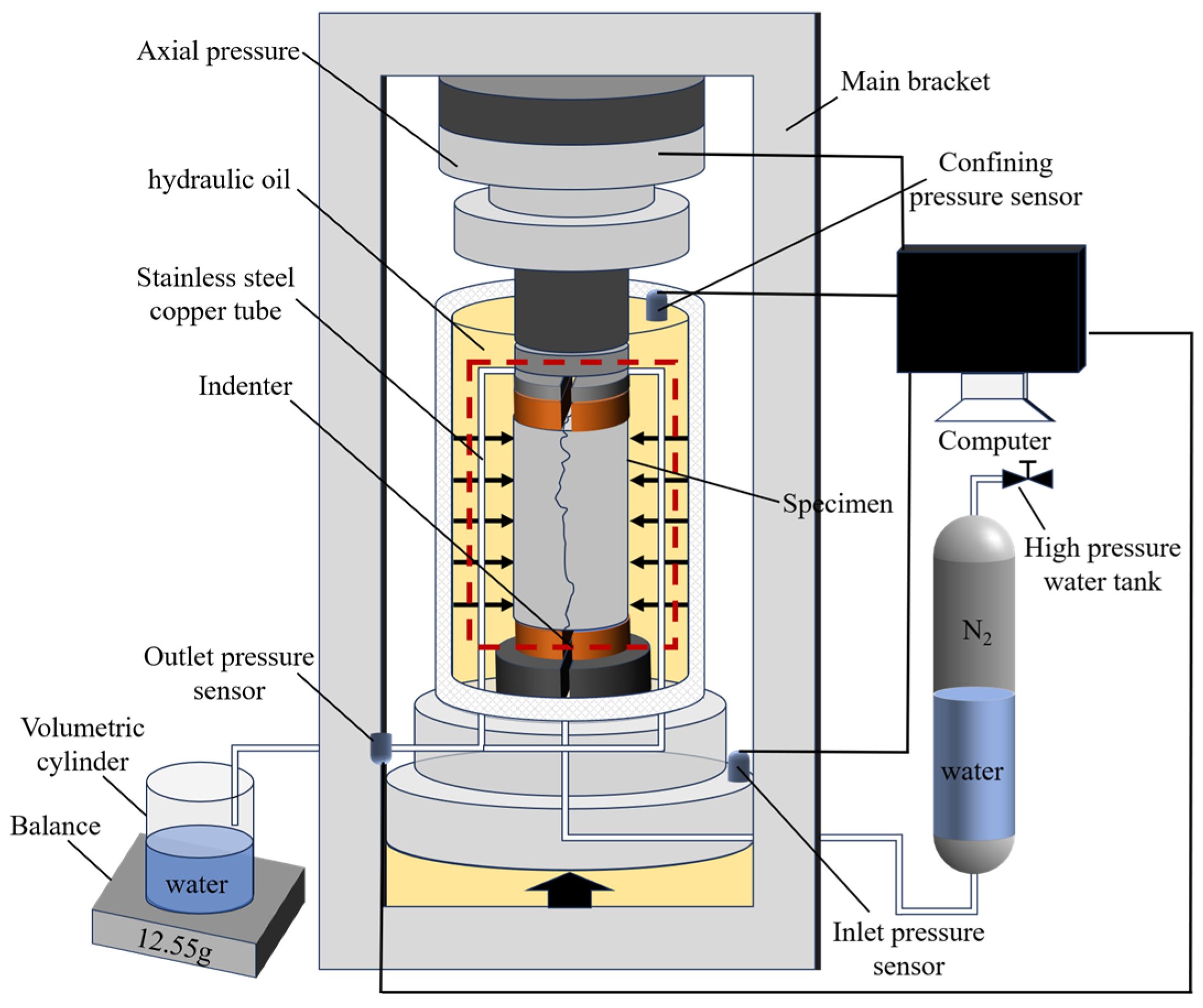
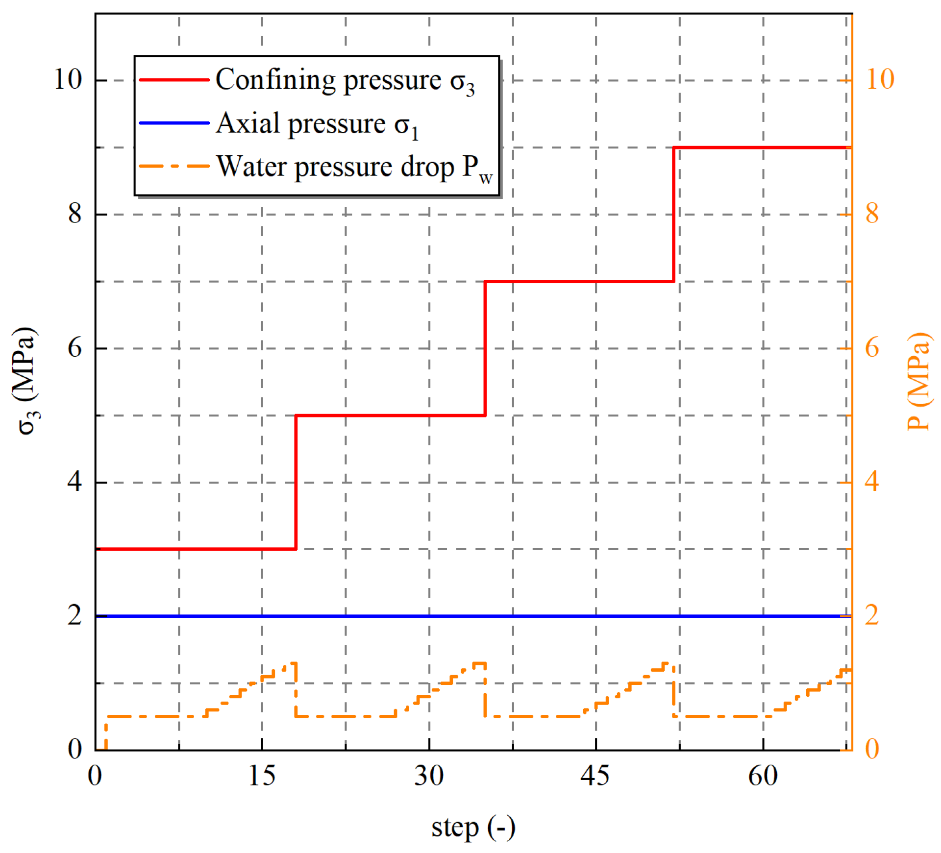
2.2. Seepage Experiment Design

The seepage tests on the sandstone specimens were conducted using an improved triaxial stress–seepage coupling test system, as shown in Figure 3. To ensure that the fluid flow remained within the laminar regime, the flow rate was maintained at a relatively low level throughout this experiment. The triaxial coupling system comprises four main components: a pressure loading unit, a fluid control unit, a system control unit, and a data acquisition unit. The system is capable of applying a maximum axial load of up to 2000 kN and confining pressure of up to 60 MPa, which fully satisfies the experimental requirements for simulating confinement and shear conditions during the seepage process. The specific experimental procedures are outlined as follows:
(1) The water-saturated sandstone specimen was connected and fixed to the collet using a heat-shrinkable tube. Internal sealing was ensured by securing the interface with a tight band. The sealed specimen was then placed into the triaxial pressure chamber;
(2) The pressure chamber was sealed by connecting it to the base using a fixture. Peripheral pressure oil was then injected into the sealed chamber. Oil injection was stopped once the chamber pressure stabilized, and continuous oil discharge was observed from the outlet, indicating full pressurization;
(3) Axial pressure was applied at a rate of 0.05 MPa/s until it reached 2 MPa to stabilize the specimen. Subsequently, the confining pressure was increased to 3 MPa at the same rate and held constant. Once the confining pressure stabilized, the valve was opened to allow for water inflow. Water pressure was then increased to the target value, and flow data were recorded after stabilization;
(4) Water pressure was incrementally increased according to the experimental protocol until all test points under the given confining pressure were completed. Thereafter, the water pressure was reduced to its minimum value;
(5) To investigate the effect of confining pressure on fracture permeability, a pressure range of 3–9 MPa was selected for the tests, which is sufficient to induce significant aperture variation in single-fracture rock masses with low directional stiffness [34,35]. The confining pressure was increased stepwise according to the loading scheme (Figure 4), and the above procedure was repeated to perform single-phase seepage tests on the fractured sandstone specimens under various confining pressure conditions. Figure 4 presents the loading procedure adopted during the seepage experiment. The figure illustrates the evolution of confining pressure (σ3), axial pressure (σ1), and water pressure drop (Pw) with respect to the loading step. The confining pressure (red line) was increased in a stepwise manner from 3 MPa to 9 MPa, simulating different in situ stress conditions. Meanwhile, the axial pressure (blue line) was held constant at 2 MPa throughout the test to ensure a stable axial boundary condition. The water pressure drops (orange dashed line) showed dynamic fluctuations corresponding to each confining pressure stage, reflecting the changing hydraulic behavior of the fracture under different stress states. This loading scheme was designed to systematically investigate the coupled response of fracture aperture evolution and seepage characteristics under increasing confinement while eliminating the influence of axial loading variations.
This study focuses on the evolution of hydraulic gradient, permeability, and the deviation of the equivalent permeability coefficient under varying confining pressures, shear displacements, and fracture surface roughness conditions. These parameters were primarily calculated based on the variations in water pressure recorded during these experiments. It is important to note that the water pressure change served solely as a basis for the calculation process, whereas the key influencing factors investigated in this study are confining pressure, shear displacement, and fracture surface roughness.

3. Theoretical Background

3.1. Governing Equations for Fluid Flow Through Rock Fracture

Conventionally, fluid flow through fractured rock is described using the finite element method (FEM) by directly solving the Navier–Stokes (N–S) equations, which form a highly coupled system of nonlinear partial differential equations, expressed as follows [36,37]:
ρ U t + U · U = P + μ 2 U + ρ f
where ρ is the fluid density; U is the velocity vector; P is the hydraulic pressure; μ is the viscous coefficient, and   f is the body force.
However, solving the highly coupled system of nonlinear partial differential equations on a standard computer is computationally intensive and time-consuming. Fluid flow in rock fractures generally involves three stages: laminar flow, transitional flow, and turbulent flow. In the laminar flow regime, the fluid behavior can be effectively characterized using a simplified analytical expression known as the cubic law [38]:
Q = w e 3 12 μ Δ P
where Q is the flow rate; w is the width of the model; e is the hydraulic aperture, which is usually obtained by measurement in the test and/or field; μ is the viscous coefficient, and Δ P is the hydraulic pressure difference between the inlet and outlet. This equation overcomes the drawback of the challenge in solving the N–S equation caused by the nonlinear term, but the geometric pattern must be smooth enough, and the fluid flow should be at low velocity. As fluid flow velocity increases, the increase in fluid flux and hydraulic gradient is no longer a linear correlation, in which the fluid flow regime is called the transition stage, and the deviation of hydraulic conductivity calculated by cubic law and the N-S equation appears. Although this deviation can be negligible at the early stage, this discrepancy should be considered when fluid flow velocity increases continuously. This nonlinear relationship between flow flux and hydraulic gradient in fractured and porous media is usually described by Forchheimer’s law [39,40], which is a zero-intercept quadratic equation:
P = A Q + B Q 2
where A and B are linear term and nonlinear term coefficients, respectively. A dimensionless parameter hydraulic gradient J , which is defined by J = P / ρ g , is applied to quantify the hydraulic pressure difference between the inlet and outlet. In this case, Equation (3) can be rewritten as
J = A Q + B Q 2
To quantitatively evaluate the influence of inertial forces in fluid flow, a dimensionless parameter E was introduced, defined as the ratio of the hydraulic pressure loss caused by inertial effects to the total pressure loss [41,42]:
E = B Q 2 A Q + B Q 2
Substituting Equations (3) and (4) into Equation (5) yields
E = B Q 2 A Q + B Q 2
Conventionally, when inertial forces contribute more than 10% to hydraulic losses, their influence becomes non-negligible, indicating the onset of nonlinear fluid flow behavior within rock fractures. The critical value of E is defined as 0.1, above which the nonlinear fluid flow should be considered in fluid dynamics analysis [43,44].

3.2. Fracture Surface Roughness Characterization

To quantify the roughness of nature in rock fracture, Barton and Choubey [45] introduce the Joint Roughness Coefficient (JRC), a widely used parameter usually in the range of 0 to 20 that is used to characterize the topography of a curve, which was calculated by [46]:
J R C = 32.2 + 32.47 lg ( Z 2 )
where Z 2 is the root mean square of the first derivative of the profile and can be obtained by
Z 2 = 1 N t δ i δ i 1 x i x i 1 2 1 / 2
For the three-dimensional fracture surface, 20 curves along the direction of fluid flow at equal intervals were selected as the samples, and the average value of their JRC was calculated to represent the roughness of the fracture surface.

4. Fluid Flow Behavior in Rock Fracture

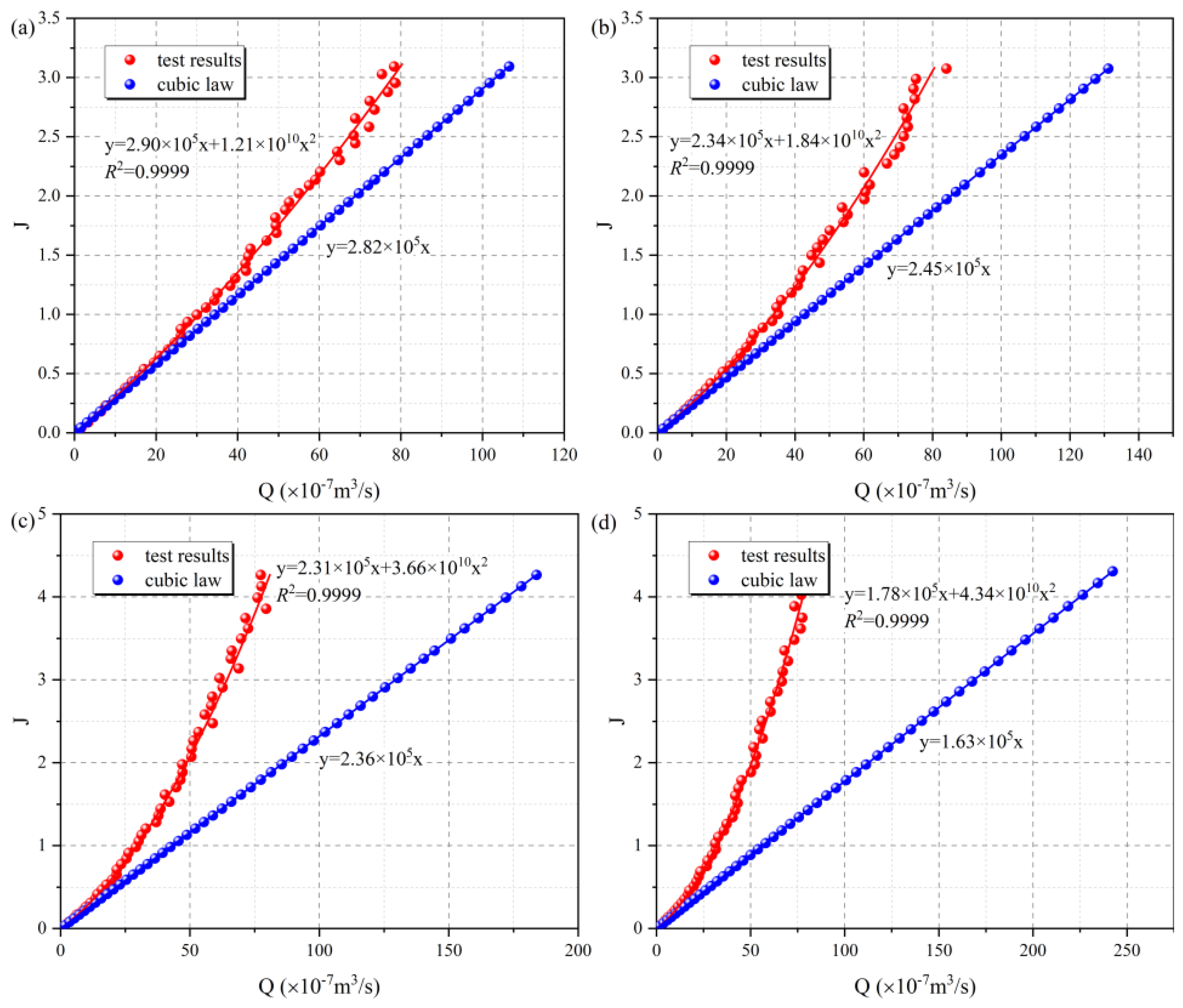
4.1. The Relationship Between the Hydraulic Gradient and Flow Flux

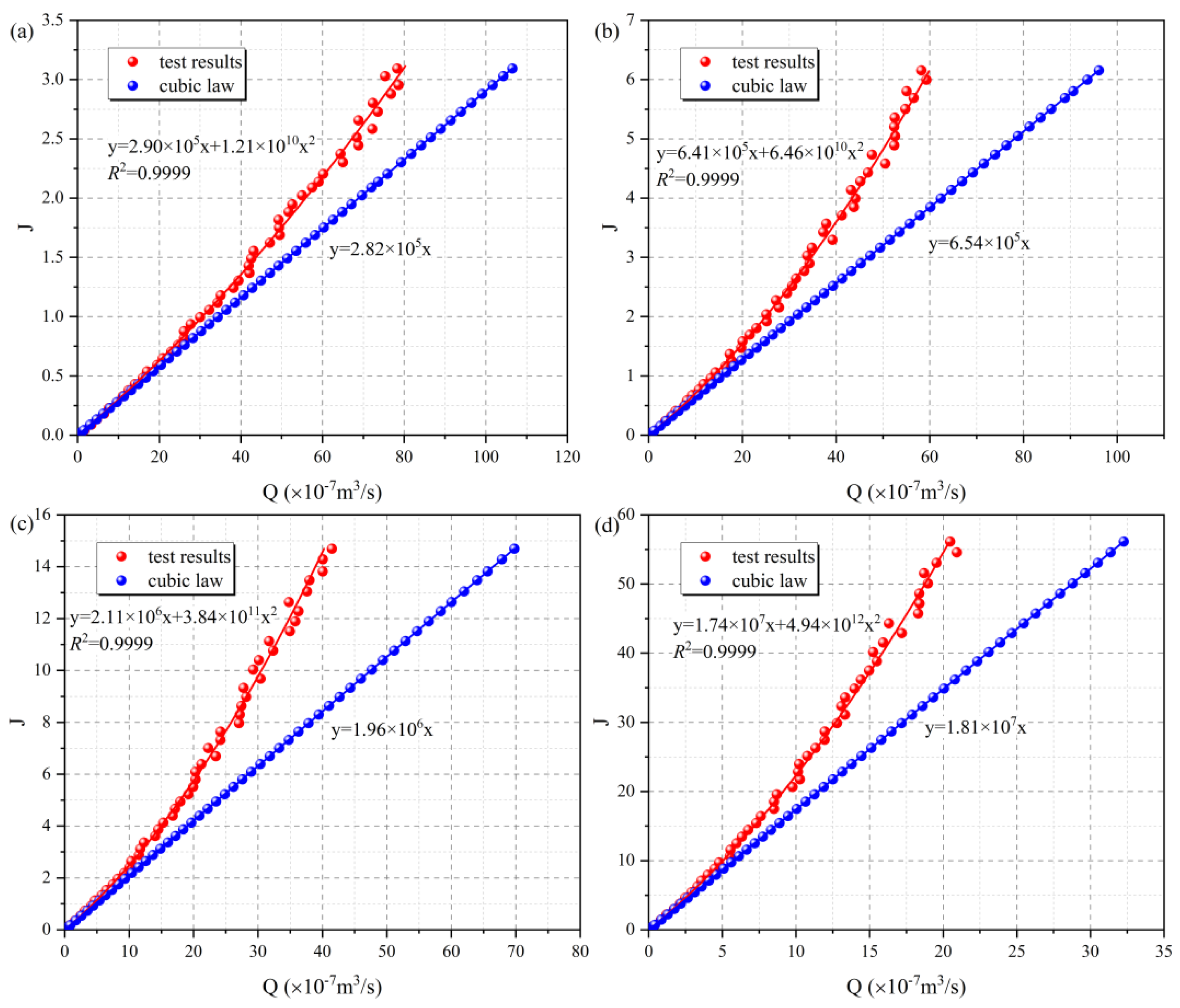
4.1.1. Effect of Confining Pressure

Given that flow flux is proportional to the cube of the fracture aperture, even a small variation in aperture can lead to a significant change in permeability. Fracture aperture can be altered by applying different confining pressures, allowing for the investigation of its effect on fluid flow behavior. Under constant confining pressure, as the flow rate increases, the flow regime may transition from linear (laminar) to nonlinear, highlighting the impact of aperture evolution on flow characteristics.
By analyzing the test data from the seepage experiments, the evolution of flow flux with respect to hydraulic gradient under different confining pressures can be quantitatively investigated. Taking the case of a fracture with a JRC value of 2.8 and a shear displacement of 0 mm as an example, the confining pressures were set to 3 MPa, 5 MPa, 7 MPa, and 9 MPa. The corresponding test results are presented in Figure 5a–d. As shown in Figure 5, the flow flux initially increases linearly with increasing hydraulic gradient, but this relationship gradually transitions into a nonlinear regime. The curvature of the flow of the flux–hydraulic gradient curve becomes more pronounced with increasing gradient, indicating a strengthening of nonlinearity. The nonlinear behavior between hydraulic gradient and flow rate becomes increasingly evident as flow conditions intensify. For comparison, permeability was also calculated using the cubic law. The deviation between the experimental results and the cubic law predictions reflects the pressure loss caused by inertial effects, represented by the nonlinear term in the Forchheimer equation. The results reveal a non-negligible discrepancy between the permeability predicted by the cubic law and derived from experimental measurements. For instance, at a confining pressure of 3 MPa and a flow rate of 80 × 10−7 m3/s, the experimentally determined hydraulic gradient is approximately 3.4, while the cubic law yields a value of 2.3—roughly 1.5 times lower than the former. This discrepancy highlights that when flow velocity (or pressure) exceeds a certain threshold, the cubic law is no longer valid for accurately estimating fracture permeability. Furthermore, as the confining pressure increases from 3 MPa to 9 MPa, the nonlinear coefficient B in the Forchheimer fitting equation also increases, indicating that the degree of nonlinearity becomes more pronounced. The detailed relationships between coefficients A and B and the confining pressure will be further discussed in a subsequent section.

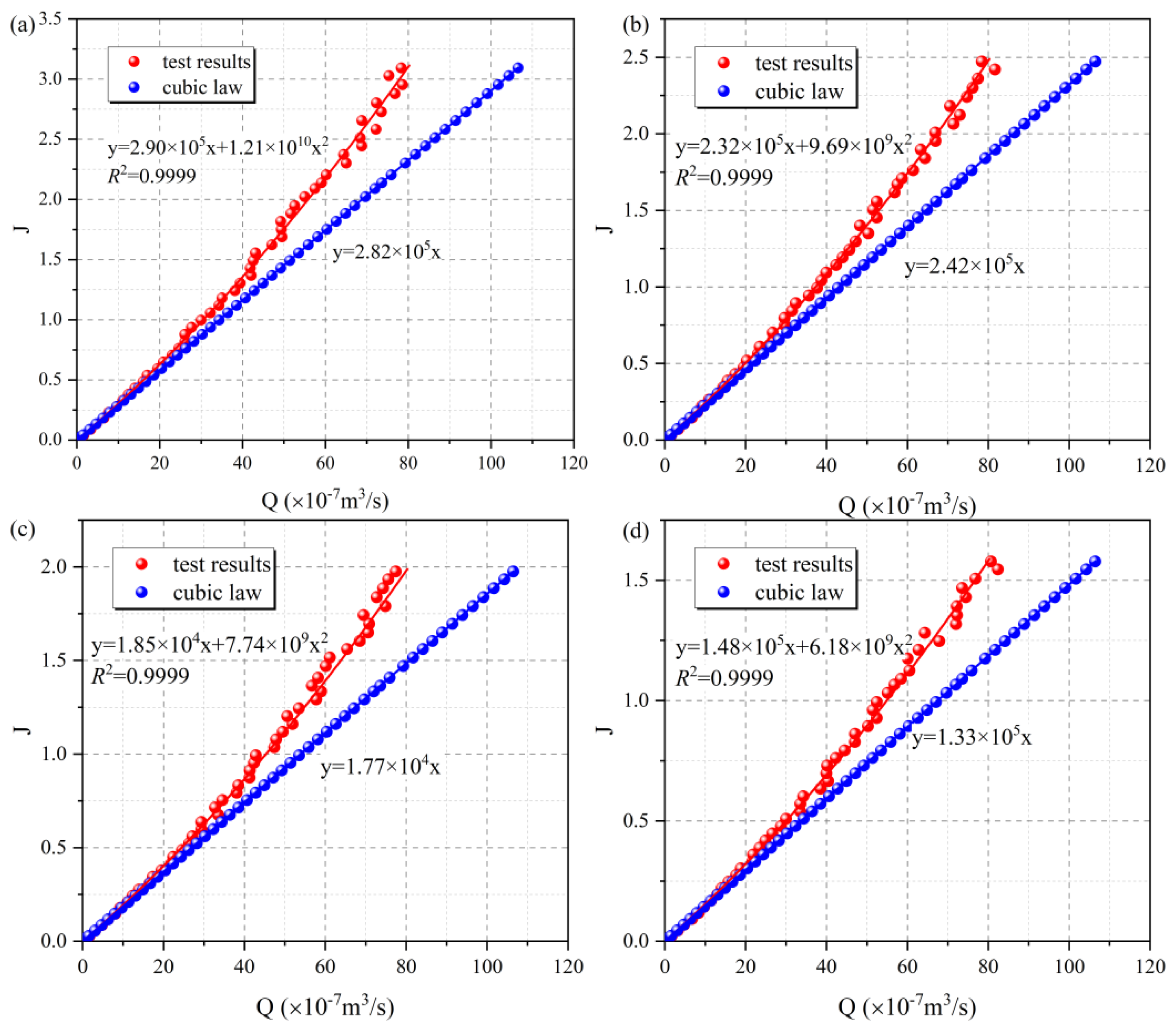
4.1.2. Effect of Shear Displacement

The selected shear displacement increments of 0, 0.5, 1.0, and 1.5 mm were designed to simulate progressive shear deformation at the joint interface under controlled laboratory conditions. While these values may appear small compared to large-scale fault movements, they are within the range of realistic in situ displacements observed in single fracture slip events, especially in the early stages of shear or in low-strain rock masses (e.g., shallow tunnels, underground openings, or excavation-induced responses). Figure 6 shows the relationship between the flow rate and hydraulic gradient under different shear displacements of JRC equal to 2.8 and confining pressure equal to 3 MPa. The result shows that the hydraulic gradient increases nonlinearly with the increase in flow rate for different shear displacements. The ratio of flow rate to hydraulic gradient is calculated simultaneously according to the cubic law, i.e., ignoring the pressure loss represented by the nonlinear term in the Forchheimer equation. The results indicate that there is a non-negligible deviation between the results obtained by the cube law and the test. As the shear displacement was set to 0.5 mm, when the flow rate is 80 × 10−7 m3/s, the hydraulic gradient obtained by the test is close to 2.5, and the value obtained by the cube law is 1.9, which is approximately 1.3 times that of the former. As the fracture shear displacement increases from 0 mm to 1.5 mm, the nonlinear term coefficient B of the fitting equation decreases, which means that the nonlinear effect is weakened. The results also show that as the shear displacement increases, the hydraulic gradient calculated at the same flow rate is smaller, which implies that an increase in shear displacement leads to an enlarged hydraulic aperture of the fracture. Regarding the concern about nonlinearities being potential artifacts of discrete testing steps, we acknowledge that a more continuous or higher-resolution shear loading regime could offer finer insights. However, the nonlinear trends observed in this study—such as abrupt changes in hydraulic conductivity and aperture evolution—are consistent with mechanical behavior reported in previous shear–flow coupling studies (e.g., fracture dilation, asperity degradation). These trends suggest that the nonlinear responses are not merely numerical artifacts but likely reflect inherent geomechanical transitions, such as asperity interlocking, damage initiation, and gouge formation.

4.1.3. Effect of Surface Roughness

Figure 7 shows the relationship between the flow rate and hydraulic gradient under different shear JRCs, with shear displacement equal to 0 mm and confining pressure equal to 3 MPa. The result shows that the pressure gradient increases nonlinearly with the increase in flow rate for different JRCs with the same shear displacement and confining pressure. Simultaneously, the ratio of flow rate to hydraulic gradient is calculated using the cubic law while neglecting the nonlinear term B of the Forchheimer equation. As JRC is equal to 7.3, when the flow rate is 80 × 10−7 m3/s, the hydraulic gradient obtained by the experiment is close to 3.0, and the value obtained by the cube law is 1.8, which is approximately 1.7 times that of the former. The results show that as the flow rate increases, the deviation that exists between the results derived from the cubic law and the test results becomes larger. As the JRC of the fracture increases from 2.8 to 17.7, the nonlinear term coefficient B of the fitting equation increases, which means that the nonlinear effect is strengthened. The results also indicate that as the JRC increases, the hydraulic gradient calculated at the same flow rate increases, implying that when the fracture is rougher, it leads to a corresponding increase in the hydraulic aperture under the same value of shear displacement.
Figure 7 illustrates the relationship between flow rate and hydraulic gradient under varying Joint Roughness Coefficients (JRCs), with a constant shear displacement of 0 mm and a confining pressure of 3 MPa. The results show that for different JRC values under identical shear displacement and confining pressure conditions, the hydraulic gradient increases nonlinearly with increasing flow rate. For comparison, the flow rate–hydraulic gradient ratio was also calculated using the cubic law, which neglects the nonlinear term B in Forchheimer’s equation. At a JRC of 7.3 and a flow rate of 80 × 10−7 m3/s, the experimentally determined hydraulic gradient is approximately 3.0, while the value predicted by the cubic law is 1.8—roughly 1.7 times lower. This growing discrepancy indicates that the deviation between cubic law predictions and experimental results becomes more pronounced with increasing flow rate. Furthermore, as the fracture JRC increases from 2.8 to 17.7, the nonlinear coefficient BBB in the Forchheimer fitting equation also increases, indicating an enhancement of nonlinear flow effects. The results also demonstrate that at the same flow rate, the hydraulic gradient increases with increasing JRC. This trend implies that rougher fracture surfaces, despite having the same shear displacement, exhibit increased flow resistance and a reduced hydraulic aperture, thereby requiring a higher-pressure gradient to maintain a given flow rate.

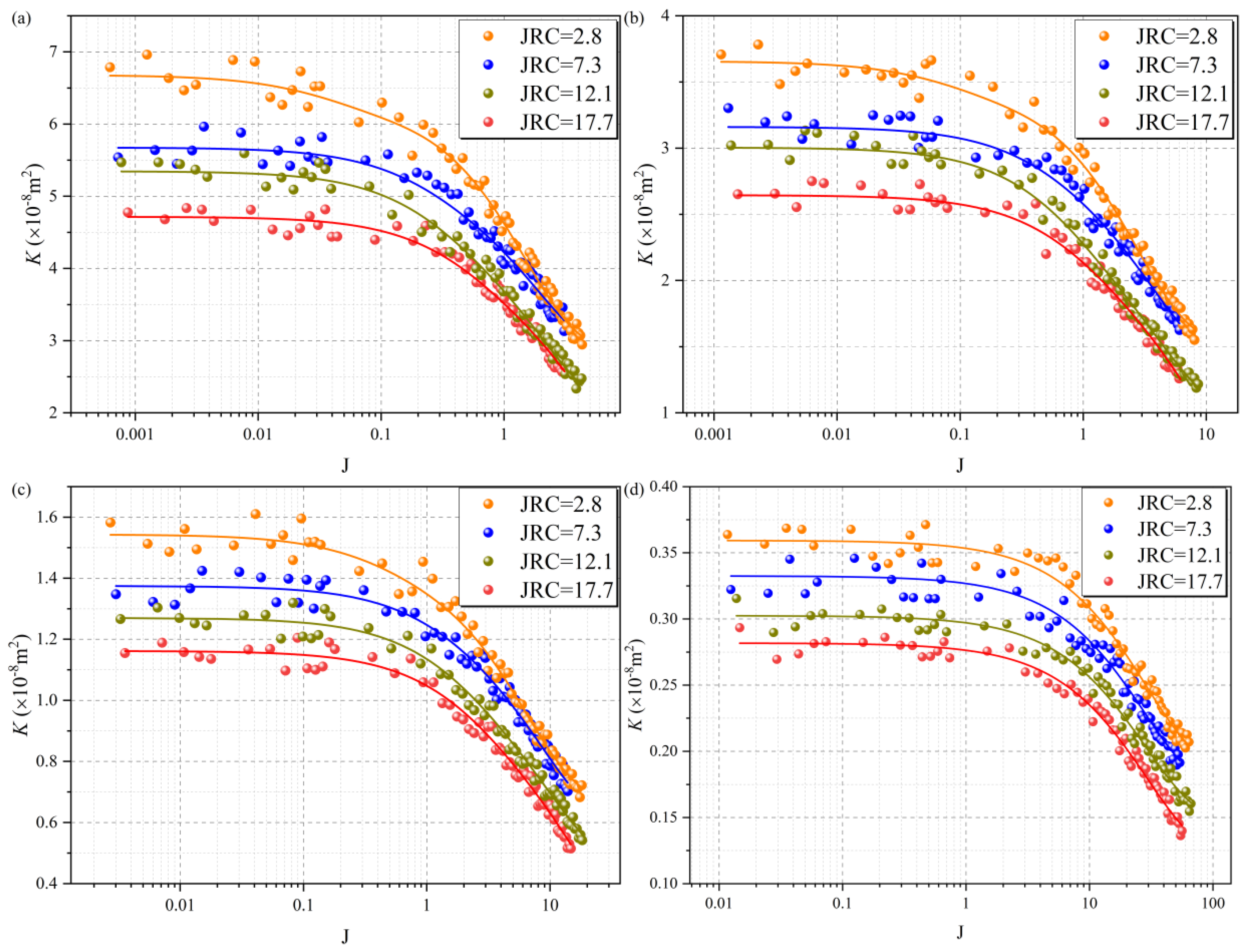
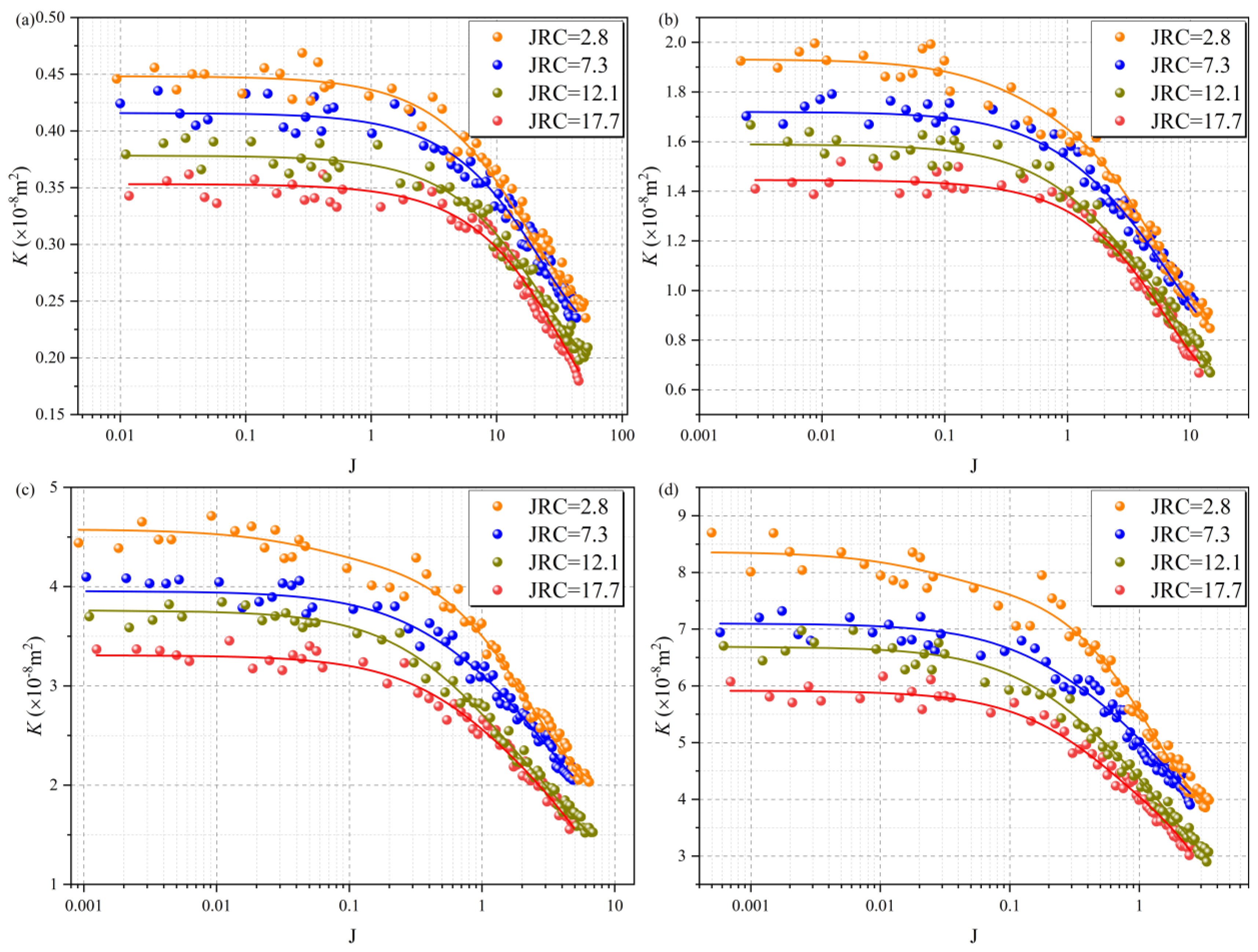
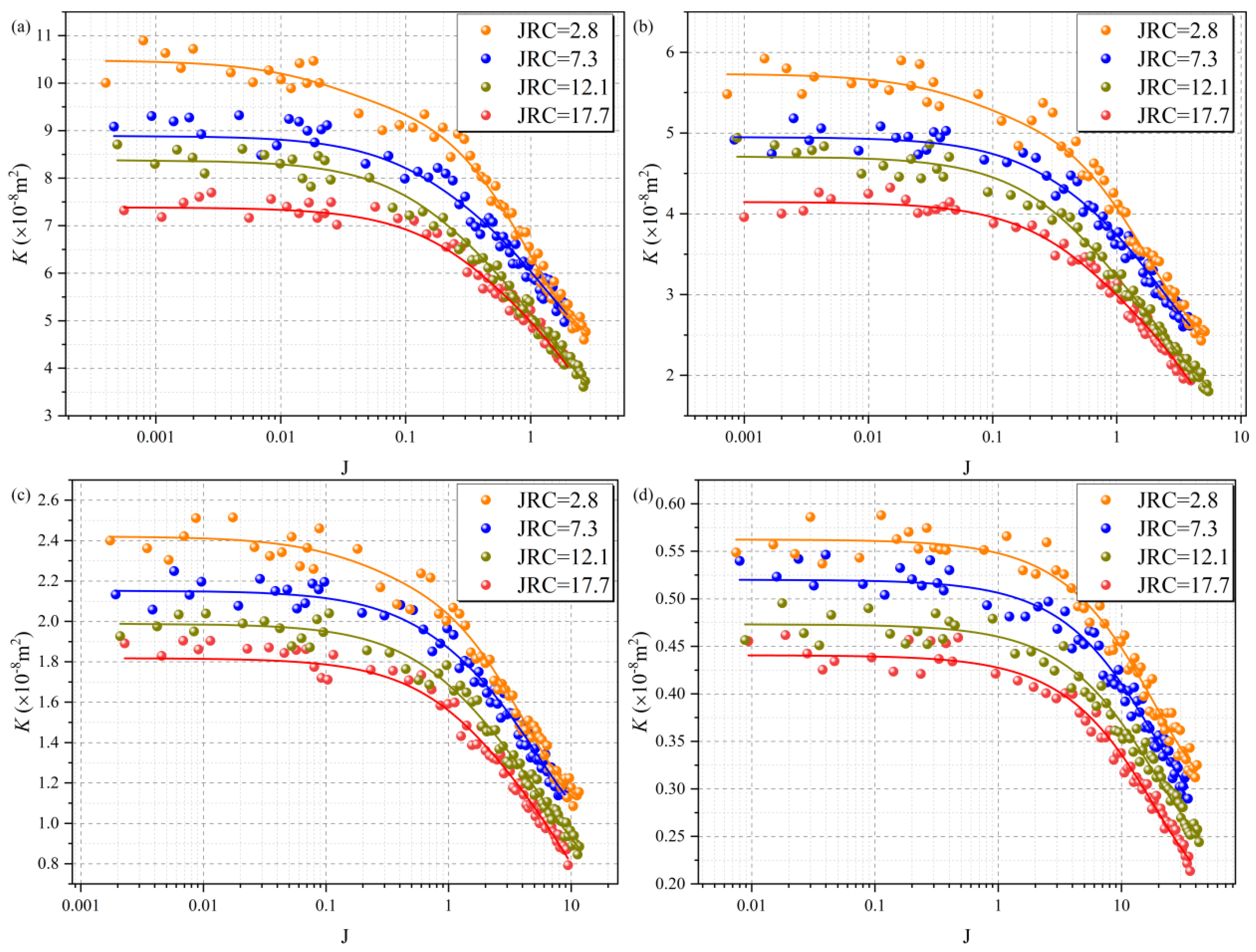
4.2. Permeability Evolution

4.2.1. Permeability Evolution Under Multivariate Conditions

To investigate the variation in permeability during the transition of fluid flow regimes, linear Darcy’s law was employed for permeability back-calculation while acknowledging that the accuracy of the calculated permeability may be limited under nonlinear flow conditions. According to Darcy’s law, the flow flux is directly proportional to the permeability, pressure gradient, and cross-sectional area of the seepage path and inversely proportional to the dynamic viscosity of the fluid. Accordingly, the permeability of the rock fracture can be back-calculated using the following expression derived from Darcy’s law:
K = μ S P Q
where S denotes the cross-section area of the outlet boundary. By calculating permeability using Equation (9), the evolution of fracture permeability under varying shear displacements, confining pressures, and surface roughness with respect to hydraulic gradient is presented in Figure 8, Figure 9, Figure 10 and Figure 11, respectively. Taking the case of a shear displacement of 0 mm as an example, the fluid remains in a laminar flow regime at low flow velocities, conforming to Darcy’s law, with permeability remaining constant. As the fluid velocity increases, weakly nonlinear flow emerges, followed by a transition to a strongly nonlinear regime at higher velocities. In this regime, the relationship between hydraulic gradient and flow rate follows Forchheimer’s equation, and the permeability K decreases sharply with increasing hydraulic gradient J. As shown in Figure 8a, permeability decreases with increasing fracture surface roughness. Additionally, the difference in permeability among specimens with varying roughness becomes less pronounced as the hydraulic gradient increases. Figure 8a–d further demonstrates that permeability gradually declines with increasing confining pressure. A comparison of Figure 8, Figure 9, Figure 10 and Figure 11 indicates that shear displacement enhances both the permeability and the emergence of nonlinear flow behavior. Moreover, increasing shear displacement leads to a more pronounced difference in permeability among fractures with different surface roughness and confining pressures, suggesting that shear displacement intensifies the impact of fracture morphology on fluid flow behavior.

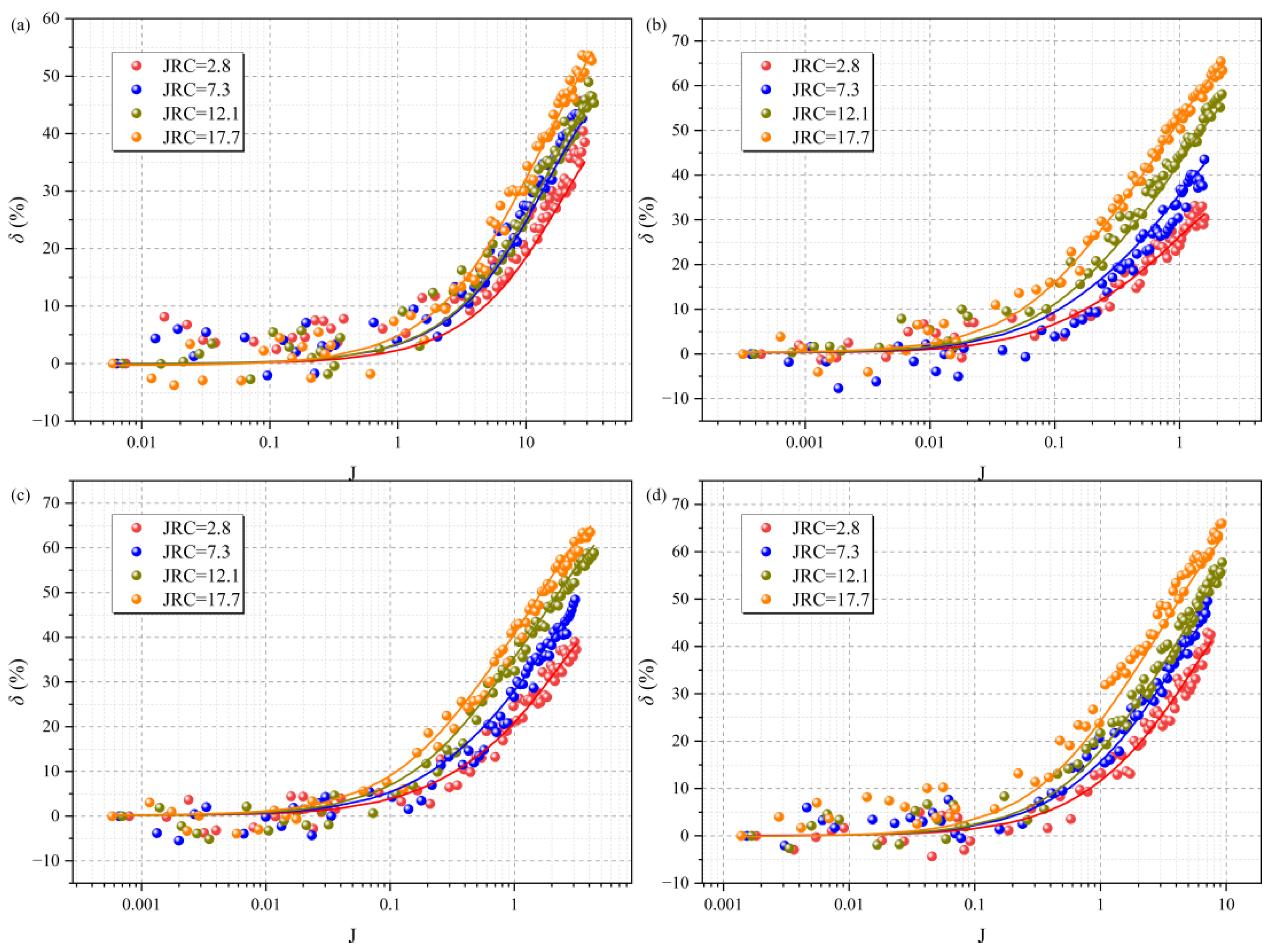
4.2.2. Quantitative Evolution of the Permeability Reduction

To quantify the impact of nonlinear effects in fluid flow on permeability, a parameter for the quantitative characteristic of the deviation of permeability obtained by experiment and cubic law is proposed, which is defined as
δ = k 0 k k 0 × 100 %
where k 0 is the permeability of the rock fracture in laminar flow, and k is the permeability of the rock fracture at an arbitrary hydraulic gradient.
Figure 12 illustrates the evolutionary trend of permeability deviation with increasing hydraulic gradient. The results show that the deviation consistently increases as the hydraulic gradient rises. At low hydraulic gradients (below approximately 0.1), the flow flux and hydraulic gradient exhibit a linear relationship, indicating laminar flow consistent with Darcy’s law, where permeability remains constant. As the hydraulic gradient increases (approximately 0.1 to 0.5), the formation of eddies introduces nonlinear behavior, transitioning the flow into a weakly nonlinear regime. With a further increase in hydraulic gradient, the fluid flow becomes strongly nonlinear, and the permeability deviation rises sharply. Specifically, Figure 12a shows that surface roughness has an insignificant effect on permeability deviation under low hydraulic gradients. However, as the gradient increases, specimens with higher JRC values exhibit larger deviations, indicating that rougher surfaces enhance the nonlinearity of fluid flow. Figure 12a–d also reveals that permeability deviation decreases with increasing confining pressure. A comparison of Figure 12, Figure 13, Figure 14 and Figure 15 indicates that permeability deviation gradually decreases as shear displacement increases. Moreover, increasing shear displacement leads to a reduction in the permeability difference among fracture specimens with varying surface roughness and confining pressure, suggesting that shear displacement contributes to homogenizing the hydraulic response of fractures.

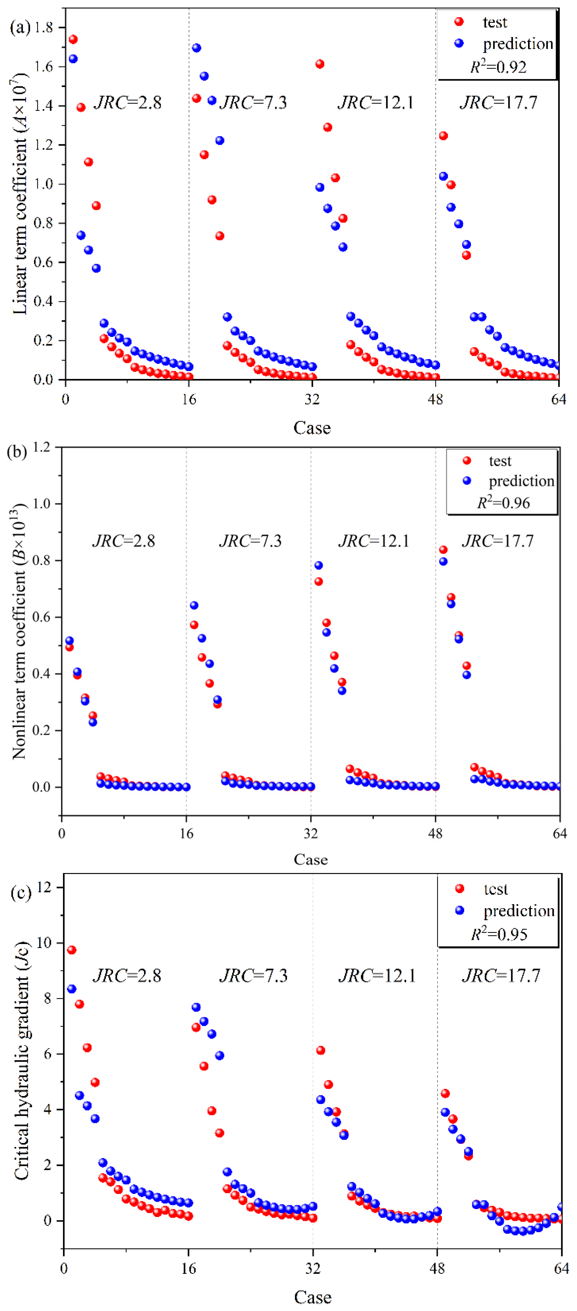
4.3. Prediction Model for Critical Hydraulic Gradient Jc and Forchheimer’s Coefficients A and B

To quantify the impact of nonlinear effects on permeability in fractured rock, a dimensionless parameter is proposed to characterize the deviation between experimentally obtained permeability and the values predicted by the cubic law. The Forchheimer coefficients A and B, derived by fitting the discrete data points on the flow flux–hydraulic gradient curves under different shear displacements, confining pressures, and fracture surface roughness conditions, are listed in Table 1. Since both confining pressure and shear displacement alter the internal void structure of the fracture, they consequently modify the hydraulic aperture. Therefore, the hydraulic aperture under varying external conditions was calculated based on the observed flow rates to represent the combined effects of confining pressure and shear displacement. The resulting hydraulic apertures are also included in Table 1. As shown in Table 1, with increasing hydraulic aperture, both coefficients A and B decrease, which is consistent with the negative exponent of aperture in Equation (11). Although the absolute magnitude of coefficient B is five orders greater than that of A, both parameters exhibit a change in approximately two orders of magnitude as the hydraulic aperture increases from 0.16 mm to 1.47 mm. The variation in coefficient A is mainly influenced by shear displacement and confining pressure, while coefficient BBB is more sensitive to the spatial distribution of fracture surface roughness and other geometrical factors. As a result, the change in B is more significant than that of A. Additionally, the critical hydraulic gradient Jc, determined in the previous section, is also summarized in Table 1. To develop a predictive model for estimating the Forchheimer coefficients A and B, as well as the critical hydraulic gradient Jc, based on hydraulic aperture (em) and Joint Roughness Coefficient (JRC), a multiple regression analysis was conducted. The resulting best-fit equations are presented as follows:
A = 9.44 × 10 5 e m 1.51 + 2.19 × 10 4 e m 1.70 × J R C B = 6.10 × 10 9 e m 3.82 + 4.32 × 10 9 e m 2.01 × J R C J c = 1.04 e m 1.14 + ( 0.27 e m + 0.17 e m 2 + 0.02 ) × J R C
By substituting the mechanical aperture and JRC into Equation (11), the predicted values of the Forchheimer coefficients A, B, and the critical hydraulic gradient Jc were obtained. To improve the accuracy and reproducibility of mechanical aperture quantification, future studies could apply computer vision to automatically extract fracture roughness and aperture evolution from high-resolution 3D scans. Deep learning models such as DeepLab [47] and EfficientNet [48] offer promising solutions. Integrating these models into geomechanical analysis may support generalized, data-driven prediction of aperture characteristics, advancing fracture. The calculated results are summarized in Table 1. Figure 16 presents a comparison between the experimentally determined and predicted values of A, B, and Jc. The coefficients of determination (R2) for all three parameters exceed 0.92, indicating that the proposed predictive equations provide consistent and accurate estimates when compared to the experimental results. The primary source of error between the predicted and measured values is attributed to isolated outliers in the simulation data, which can hinder the fitting accuracy of the regression model [49,50].
Table 1. The simulation (T) and prediction (P) values of A, B, and Jc.
NoShear
(mm)
Pressure
(MPa)
em
(mm)
JRCA(T)B(T)Jc(T)A(P)B(P)Jc(P)
10.090.162.81.74 × 1074.94 × 10129.75 1.64 × 1077.17 × 10128.35
20.590.272.81.39 × 1073.95 × 10127.79 7.39 × 1061.07 × 10124.51
31.090.292.81.11 × 1073.16 × 10126.23 6.62 × 1068.36 × 10114.14
41.590.322.88.90 × 1062.53 × 10124.98 5.70 × 1065.93 × 10113.67
50.070.52.82.11 × 1063.84 × 10111.54 2.89 × 1061.35 × 10112.09
60.570.562.81.68 × 1063.07 × 10111.40 2.43 × 1069.47 × 10101.80
71.070.612.81.35 × 1062.46 × 10111.12 2.13 × 1067.30 × 10101.60
81.570.652.81.08 × 1061.96 × 10110.79 1.94 × 1066.04 × 10101.47
90.050.782.86.41 × 1056.46 × 10100.68 1.47 × 1063.57 × 10101.14
100.550.842.85.12 × 1055.17 × 10100.54 1.31 × 1062.90 × 10101.03
111.050.92.84.09 × 1054.13 × 10100.43 1.18 × 1062.41 × 10100.93
121.550.972.83.27 × 1053.30 × 10100.30 1.05 × 1061.97 × 10100.85
130.031.042.82.90 × 1051.21 × 10100.38 9.47 × 1051.64 × 10100.78
140.531.122.82.32 × 1059.69 × 1090.26 8.46 × 1051.36 × 10100.72
151.031.212.81.86 × 1057.74 × 1090.24 7.52 × 1051.12 × 10100.68
161.531.312.81.48 × 1056.18 × 1090.17 6.67 × 1059.20 × 1090.65
170.090.177.31.44 × 1075.73 × 10126.96 1.70 × 1076.42 × 10127.69
180.590.187.31.15 × 1074.58 × 10125.57 1.55 × 1075.26 × 10127.18
191.090.197.39.20 × 1063.67 × 10123.96 1.43 × 1074.36 × 10126.72
201.590.217.37.35 × 1062.93 × 10123.16 1.22 × 1073.09 × 10125.95
210.070.57.31.75 × 1064.15 × 10111.15 3.21 × 1062.13 × 10111.76
220.570.597.31.40 × 1063.32 × 10110.92 2.49 × 1061.37 × 10111.31
231.070.637.31.12 × 1062.66 × 10110.74 2.25 × 1061.15 × 10111.16
241.570.687.38.92 × 1052.12 × 10110.50 2.00 × 1069.51 × 10100.99
250.050.837.35.22 × 1057.86 × 10100.42 1.47 × 1065.83 × 10100.65
260.550.897.34.17 × 1056.28 × 10100.34 1.32 × 1064.94 × 10100.56
271.050.967.33.33 × 1055.03 × 10100.27 1.18 × 1064.14 × 10100.49
281.551.047.32.66 × 1054.02 × 10100.22 1.04 × 1063.44 × 10100.43
290.031.117.32.35 × 1051.84 × 10100.24 9.40 × 1052.97 × 10100.41
300.531.197.31.88 × 1051.47 × 10100.19 8.45 × 1052.54 × 10100.41
311.031.297.31.50 × 1051.18 × 10100.15 7.46 × 1053.36 × 10100.45
321.531.397.31.20 × 1059.41 × 1090.10 6.65 × 1052.87 × 10100.52
330.090.2612.11.61 × 1077.26 × 10126.13 9.83 × 1061.83 × 10124.36
340.590.2812.11.29 × 1075.81 × 10124.90 8.76 × 1061.46 × 10123.93
351.090.312.11.03 × 1074.64 × 10123.92 7.87 × 1061.19 × 10123.55
361.590.3312.18.25 × 1063.71 × 10123.13 6.78 × 1069.07 × 10113.07
370.070.5312.11.79 × 1066.52 × 10110.89 3.24 × 1062.56 × 10111.23
380.570.5712.11.43 × 1065.22 × 10110.71 2.90 × 1062.14 × 10111.02
391.070.6212.11.15 × 1064.18 × 10110.57 2.54 × 1061.75 × 10110.80
401.570.6712.19.15 × 1053.34 × 10110.45 2.25 × 1061.45 × 10110.62
410.050.8112.15.26 × 1051.45 × 10110.30 1.68 × 1069.35 × 10100.27
420.550.8812.14.20 × 1051.16 × 10110.24 1.47 × 1067.75 × 10100.16
431.050.9412.13.35 × 1059.25 × 10100.19 1.33 × 1066.69 × 10100.10
441.551.0212.12.68 × 1057.40 × 10100.15 1.17 × 1065.59 × 10100.07
450.031.0812.12.32 × 1053.66 × 10100.17 1.07 × 1064.93 × 10100.07
460.531.2112.11.85 × 1052.93 × 10100.13 9.00 × 1053.86 × 10100.14
471.031.2612.11.48 × 1052.34 × 10100.11 8.45 × 1053.54 × 10100.19
481.531.3612.11.18 × 1051.87 × 10100.09 7.50 × 1054.31 × 10100.34
490.090.2717.71.25 × 1078.38 × 10124.58 1.04 × 1071.97 × 10123.91
500.590.317.79.97 × 1066.71 × 10123.66 8.82 × 1061.47 × 10123.29
511.090.3217.77.97 × 1065.36 × 10122.93 7.96 × 1061.23 × 10122.94
521.590.3517.76.36 × 1064.29 × 10122.34 6.92 × 1069.67 × 10112.49
530.070.5717.71.44 × 1067.08 × 10110.59 3.21 × 1062.89 × 10110.58
540.570.5717.71.15 × 1065.66 × 10110.47 3.21 × 1062.89 × 10110.58
551.070.6617.79.16 × 1054.53 × 10110.38 2.55 × 1062.06 × 10110.18
561.570.7217.77.31 × 1053.63 × 10110.30 2.23 × 1061.69 × 1011−0.01
570.050.8717.73.98 × 1051.48 × 10110.18 1.66 × 1061.12 × 1011−0.31
580.550.9317.73.18 × 1051.19 × 10110.15 1.49 × 1069.65 × 1010−0.36
591.051.0117.72.53 × 1059.50 × 10100.12 1.31 × 1068.08 × 1010−0.38
601.551.0917.72.02 × 1057.60 × 10100.09 1.16 × 1066.87 × 1010−0.34
610.031.1717.71.78 × 1054.34 × 10100.10 1.04 × 1065.91 × 1010−0.25
620.531.2617.71.42 × 1053.47 × 10100.08 9.28 × 1055.06 × 1010−0.09
631.031.3517.71.13 × 1052.78 × 10100.06 8.33 × 1054.38 × 10100.12
641.531.4717.79.02 × 1042.23 × 10100.05 7.29 × 1053.66 × 10100.50

5. Conclusions

This study conducted a series of systematic seepage experiments on rock fractures with varying surface roughness, confining pressures, and shear displacements to investigate nonlinear fluid flow behavior and identify the critical threshold for the transition from laminar to nonlinear regimes. Fracture specimens were prepared through drilling, cutting, polishing, and Brazilian splitting. The surface morphology of the fractures was characterized using a 3D surface scanner, and the Joint Roughness Coefficient (JRC) was calculated. Four representative fracture types with JRC values of 2.8, 7.1, 12.1, and 17.7 were selected. A total of 64 seepage tests were performed under four confining pressures (3, 5, 7, and 9 MPa) and four shear displacements (0, 0.5, 1.0, and 1.5 mm).
The results indicate that at low hydraulic gradients, flow behavior adheres to Darcy’s law, with constant permeability and a linear relationship between flow rate and hydraulic gradient. As the gradient increases, weak nonlinearity emerges due to the formation of eddies and additional energy loss, causing a progressive decrease in permeability. The onset of nonlinear flow occurs earlier under higher surface roughness, increased confining pressure, and larger shear displacement, suggesting that these factors jointly lower the nonlinear threshold. The Forchheimer equation proved to be a reliable model for describing fluid flow beyond the linear regime. A critical hydraulic gradient Jc, defined as the point where inertial energy loss accounts for 10% of the total energy loss, was introduced to distinguish between laminar and nonlinear flow. Below Jc, the cubic law provides a simplified and efficient approximation; beyond this threshold, the Forchheimer equation should be applied, with coefficients A and B determined from empirical correlations. This study established predictive models for A, B, and Jc, using hydraulic aperture and JRC as input variables. These models achieved high prediction accuracy (R2 > 0.92), offering practical tools for evaluating nonlinear seepage characteristics in fractured media.
While this study offers a quantitative analysis of nonlinear flow in rock fractures, certain limitations remain. Scale effects, flow anisotropy, and surface contact mechanics were not incorporated. In addition, the roles of shear displacement and confining pressure were examined only indirectly through aperture variation, without addressing the coupled interactions between mechanical loading and fluid transport. In addition, due to experimental constraints, this study only considered fracture apertures ranging from 0.16 mm to 1.47 mm. It remains unclear whether the nonlinear flow coefficients for a wider range of fracture apertures can be accurately predicted using the current model. In future work, we intend to incorporate a broader spectrum of experimental conditions to develop more generalized predictive approaches. Future work will aim to address these limitations by incorporating high-resolution CT reconstruction and coupled PFC-CFD modeling, enabling a more comprehensive understanding of the coupled stress–flow–structure behavior in fractured rock systems.

Author Contributions

H.P., investigation, formal analysis, writing—original draft preparation, data curation, software, validation; Y.C., writing—review and editing, data curation, investigation, supervision; K.X., conceptualization, methodology, software, data curation; S.Z., writing—review and editing, data curation; X.H., writing—review and editing, formal analysis, software, validation; J.X., writing—review and editing, data curation, formal analysis, software, validation. All authors have read and agreed to the published version of the manuscript.

Funding

This study was financially supported by the Xinjiang Uygur Autonomous Region Science and Technology Major Program (Grant No. 2023A01002), National Natural Science Foundation of China (Grant No. 52374147, 42207180), China Postdoctoral Science Foundation (Grant No. 2024M753531), and Jiangsu Funding Program for Excellent Postdoctoral Talent (Grant No. 2024ZB853).

Data Availability Statement

The data that support the findings of this study are available from the corresponding author upon request.

Conflicts of Interest

The authors declare no conflict of interest.

References

  1. Gao, X.; Yeh, T.C.J.; Yan, E.C.; Wang, W.; Cai, J.; Liang, Y.; Ge, J.; Qi, Y.; Hao, Y. Fusion of hydraulic tomography and displacement back analysis for underground cavern stability investigation. Water Resour. Res. 2018, 54, 8632–8652. [Google Scholar] [CrossRef]
  2. Zhu, L.; Yang, Q.; Luo, L.; Cui, S. Pore-water pressure model for carbonate fault materials based on cyclic triaxial tests. Front. Earth Sci. 2022, 10, 842765. [Google Scholar] [CrossRef]
  3. Yang, Y.; Feng, H.; Zhang, Y.; Wang, Y.; Ma, M.; Zhu, P. Mechanical properties and brittleness characterization method of low-rank coal and its char particles under a uniaxial compression test. Energy Fuels 2023, 37, 7696–7706. [Google Scholar] [CrossRef]
  4. Nie, Z.; Chen, J.; Zhang, W.; Tan, C.; Ma, Z.; Wang, F.; Zhang, Y.; Que, J. A new method for three-dimensional fracture network modelling for trace data collected in a large sampling window. Rock Mech. Rock Eng. 2020, 53, 1145–1161. [Google Scholar] [CrossRef]
  5. Huang, N.; Jiang, Y.; Li, B.; Liu, R. A numerical method for simulating fluid flow through 3-D fracture networks. J. Nat. Gas Sci. Eng. 2016, 33, 1271–1281. [Google Scholar] [CrossRef]
  6. Kim, S.Y.; Koo, J.-M.; Kuznetsov, A.V. Effect of anisotropy in permeability and effective thermal conductivity on thermal performance of an aluminum foam heat sink. Numer. Heat Transfer. 2001, 40, 21–36. [Google Scholar] [CrossRef]
  7. Tang, H.; Lin, B.; Wang, D. Granular collapse in fluids: Dynamics and flow regime identification. Particuology 2024, 92, 30–41. [Google Scholar] [CrossRef]
  8. Xiong, F.; Jiang, Q.; Ye, Z.; Zhang, X. Nonlinear flow behavior through rough-walled rock fractures: The effect of contact area. Comput. Geotech. 2018, 102, 179–195. [Google Scholar] [CrossRef]
  9. Wang, M.; Chen, Y.-F.; Ma, G.-W.; Zhou, J.-Q.; Zhou, C.-B. Influence of surface roughness on nonlinear flow behaviors in 3D self-affine rough fractures: Lattice Boltzmann simulations. Adv. Water Resour. 2016, 96, 373–388. [Google Scholar] [CrossRef]
  10. Gong, J.; Rossen, W.R. Modeling flow in naturally fractured reservoirs: Effect of fracture aperture distribution on dominant sub-network for flow. Pet. Sci. 2017, 14, 138–154. [Google Scholar] [CrossRef]
  11. Sudarja; Haq, A.; Deendarlianto; Indarto; Widyaparaga, A. Experimental study on the flow pattern and pressure gradient of air-water two-phase flow in a horizontal circular mini-channel. J. Hydrodyn. 2019, 31, 102–116. [Google Scholar] [CrossRef]
  12. Pu, H.; Xue, K.; Wu, Y.; Zhang, S.; Liu, D.; Xu, J. Estimating the permeability of fractal rough rock fractures with variable apertures under normal and shear stresses. Phys. Fluids 2025, 37, 036635. [Google Scholar] [CrossRef]
  13. Zhao, Z.; Jing, L.; Neretnieks, I.; Moreno, L. Analytical solution of coupled stress-flow-transport processes in a single rock fracture. Comput. Geosci. 2011, 37, 1437–1449. [Google Scholar] [CrossRef]
  14. Wu, X.; Gao, Z.; Meng, H.; Wang, Y.; Cheng, C. Experimental study on the uniform distribution of gas-liquid two-phase flow in a variable-aperture deflector in a parallel flow heat exchanger. Int. J. Heat Mass Transf. 2020, 150, 119353. [Google Scholar] [CrossRef]
  15. Wang, C.; Jiang, Y.; Gao, R.; Wang, X. On the evolution of relative permeability of two-phase flow in rock fractures: The effect of aperture distribution. IOP Conf. Ser. Earth Environ. Sci. 2021, 861, 042112. [Google Scholar] [CrossRef]
  16. Rong, G.; Yang, J.; Cheng, L.; Zhou, C. Laboratory investigation of nonlinear flow characteristics in rough fractures during shear process. J. Hydrol. 2016, 541, 1385–1394. [Google Scholar] [CrossRef]
  17. Zhou, J.-Q.; Wang, M.; Wang, L.; Chen, Y.-F.; Zhou, C.-B. Emergence of nonlinear laminar flow in fractures during shear. Rock Mech. Rock Eng. 2018, 51, 3635–3643. [Google Scholar] [CrossRef]
  18. Yang, J.; Wang, Z.; Qiao, L.; Li, W.; Liu, J. Effects of roughness and aperture on mesoscopic and macroscopic flow characteristics in rock fractures. Environ. Earth Sci. 2023, 82, 594.1–594.16. [Google Scholar] [CrossRef]
  19. Wang, Z.; Xu, C.; Dowd, P. A Modified Cubic Law for single-phase saturated laminar flow in rough rock fractures. Int. J. Rock Mech. Min. Sci. Géoméch. Abstr. 2018, 103, 107–115. [Google Scholar] [CrossRef]
  20. Javadi, M.; Sharifzadeh, M.; Shahriar, K.; Mitani, Y. Critical Reynolds number for nonlinear flow through rough-walled fractures: The role of shear processes. Water Resour. Res. 2014, 50, 1789–1804. [Google Scholar] [CrossRef]
  21. Xue, K.; Pu, H.; Li, M.; Luo, P.; Liu, D.; Yi, Q. Fractal-based analysis of stress-induced dynamic evolution in geometry and permeability of porous media. Phys. Fluids 2025, 37, 036630. [Google Scholar] [CrossRef]
  22. Lee, S.H.; Lee, K.; Yeo, I.W. Assessment of the validity of Stokes and Reynolds equations for fluid flow through a rough-walled fracture with flow imaging. Geophys. Res. Lett. 2014, 41, 4578–4585. [Google Scholar] [CrossRef]
  23. Huang, N.; Jiang, Y.; Liu, R.; Li, B.; Sugimoto, S. A novel three-dimensional discrete fracture network model for investigating the role of aperture heterogeneity on fluid flow through fractured rock masses. Int. J. Rock Mech. Min. Sci. Géoméch. Abstr. 2019, 116, 25–37. [Google Scholar] [CrossRef]
  24. Ishibashi, T.; Watanabe, N.; Hirano, N.; Okamoto, A.; Tsuchiya, N. Beyond-laboratory-scale prediction for channeling flows through subsurface rock fractures with heterogeneous aperture distributions revealed by laboratory evaluation. J. Geophys. Res. Solid Earth 2015, 120, 106–124. [Google Scholar] [CrossRef]
  25. Lee, H.S.; Cho, T.F. Hydraulic characteristics of rough fractures in linear flow under normal and shear load. Rock Mech. Rock Eng. 2002, 35, 299–318. [Google Scholar] [CrossRef]
  26. Zhang, Y.; Chai, J. Effect of surface morphology on fluid flow in rough fractures: A review. J. Nat. Gas Sci. Eng. 2020, 79, 103343. [Google Scholar] [CrossRef]
  27. Zou, L.; Jing, L.; Cvetkovic, V. Roughness decomposition and nonlinear fluid flow in a single rock fracture. Int. J. Rock Mech. Min. Sci. Géoméch. Abstr. 2015, 75, 102–118. [Google Scholar] [CrossRef]
  28. Hansen, C.; Yang, X.I.A.; Abkar, M. Data-driven dynamical system models of roughness-induced secondary flows in thermally stratified turbulent boundary layers. J. Fluids Eng. 2023, 145, 061102. [Google Scholar] [CrossRef]
  29. Vilarrasa, V.; Koyama, T.; Neretnieks, I.; Jing, L. Shear-induced flow channels in a single rock fracture and their effect on solute transport. Transp. Porous Media 2011, 87, 503–523. [Google Scholar] [CrossRef]
  30. Zareidarmiyan, A.; Parisio, F.; Makhnenko, R.Y.; Salarirad, H.; Vilarrasa, V. How equivalent are equivalent porous media? Geophys. Res. Lett. 2011, 38, L24401. [Google Scholar] [CrossRef]
  31. Xiong, F.; Jiang, Q.; Xu, C.; Zhang, X.; Zhang, Q. Influences of connectivity and conductivity on nonlinear flow behaviours through three-dimension discrete fracture networks. Comput. Geotech. 2019, 107, 128–141. [Google Scholar] [CrossRef]
  32. Hu, B.; Wang, J.G.; Sun, R.; Zhao, Z. A permeability model for the fractal tree-like fracture network with self-affine surface roughness in shale gas reservoirs. Géoméch. Geophys. Geo-Energy Geo-Resour. 2024, 10, 24. [Google Scholar] [CrossRef]
  33. Xue, K.; Zhang, Z.; Hao, S.; Luo, P.; Wang, Y. On the onset of nonlinear fluid flow transition in rock fracture network: Theoretical and computational fluid dynamic investigation. Phys. Fluids 2022, 34, 125114. [Google Scholar] [CrossRef]
  34. Wang, Y.; Zhang, Z.; Liu, X.; Xue, K. Relative permeability of two-phase fluid flow through rough fractures: The roles of fracture roughness and confining pressure. Adv. Water Resour. 2023, 175, 104426. [Google Scholar] [CrossRef]
  35. Liu, X.; Xue, K.; Luo, Y.; Long, K.; Liu, Y.; Liang, Z. The Effect of Pore Pressure on the Mechanical Behavior of Coal with Burst Tendency at a Constant Effective Stress. Sustainability 2022, 14, 14568. [Google Scholar] [CrossRef]
  36. de Dreuzy, J.; Méheust, Y.; Pichot, G. Influence of fracture scale heterogeneity on the flow properties of three-dimensional discrete fracture networks (DFN). J. Geophys. Res. Solid Earth 2012, 117. [Google Scholar] [CrossRef]
  37. Luo, Y.; Zhang, Z.; Zhang, L.; Xue, K.; Long, K. Influence of fracture roughness and void space morphology on nonlinear fluid flow through rock fractures Concept Discrete Fracture Network Model Simulator. Eur. Phys. J. Plus. 2022, 137. [Google Scholar] [CrossRef]
  38. Ju, Y.; Dong, J.; Gao, F.; Wang, J. Evaluation of water permeability of rough fractures based on a self-affine fractal model and optimized segmentation algorithm. Adv. Water Resour. 2019, 129, 99–111. [Google Scholar] [CrossRef]
  39. Ji, S.; Lee, H.; Yeo, I.W.; Lee, K. Effect of nonlinear flow on DNAPL migration in a rough-walled fracture. Water Resour. Res. 2008, 44, 636–639. [Google Scholar] [CrossRef]
  40. Zhou, J.-Q.; Hu, S.-H.; Fang, S.; Chen, Y.-F.; Zhou, C.-B. Nonlinear flow behavior at low Reynolds numbers through rough-walled fractures subjected to normal compressive loading. Int. J. Rock Mech. Min. Sci. Géoméch. Abstr. 2015, 80, 202–218. [Google Scholar] [CrossRef]
  41. Javadi, M.; Sharifzadeh, M.; Shahriar, K. A new geometrical model for non-linear fluid flow through rough fractures. J. Hydrol. 2010, 389, 18–30. [Google Scholar] [CrossRef]
  42. Chen, Z.; Qian, J.; Qin, H. Experimental study of the non-Darcy flow and solute transport in a channeled single fracture. J. Hydrodyn. 2011, 23, 745–751. [Google Scholar] [CrossRef]
  43. Qian, J.; Chen, Z.; Zhan, H.; Guan, H. Experimental study of the effect of roughness and Reynolds number on fluid flow in rough-walled single fractures: A check of local cubic law. Hydrol. Process. 2011, 25, 614–622. [Google Scholar] [CrossRef]
  44. Zou, L.; Jing, J.; Cvetkovic, V. Shear-enhanced nonlinear flow in rough-walled rock fractures. Int. J. Rock Mech. Min. Sci. 2017, 97, 33–45. [Google Scholar] [CrossRef]
  45. Barton, N.; Choubey, V. The shear strength of rock joints in theory and practice. Rock Mech. Rock Eng. 1977, 10, 1–54. [Google Scholar] [CrossRef]
  46. Tse, R.; Cruden, D. Estimating joint roughness coefficients. Int. J. Rock Mech. Min. Sci. Géoméch. Abstr. 1979, 16, 303–307. [Google Scholar] [CrossRef]
  47. Kabir, H.; Wu, J.; Dahal, S.; Joo, T.; Garg, N. Automated estimation of cementitious sorptivity via computer vision. Nat. Commun. 2024, 15, 9935. [Google Scholar] [CrossRef]
  48. Song, Z.; Zou, S.; Zhou, W.; Huang, Y.; Shao, L.; Yuan, J.; Gou, X.; Jin, W.; Wang, Z.; Chen, X.; et al. Clinically applicable histopathological diagnosis system for gastric cancer detection using deep learning. Nat. Commun. 2020, 11, 4294. [Google Scholar] [CrossRef]
  49. Aguirre, L.A.; Barbosa, B.H.; Braga, A.P. Prediction and simulation errors in parameter estimation for nonlinear systems. Mech. Syst. Signal Process. 2010, 24, 2855–2867. [Google Scholar] [CrossRef]
  50. Oberkampf, W.L. Simulation Accuracy, Uncertainty, and Predictive Capability: A Physical Sciences Perspective. In Computer Simulation Validation: Fundamental Concepts, Methodological Frameworks, and Philosophical Perspectives; Beisbart, C., Saam, N.J., Eds.; Springer International Publishing: Cham, Switzerland, 2019; pp. 69–97. [Google Scholar]
Figure 1. Preparation process of shale standard specimen: (a) drilling; (b) cutting; (c) polish; (d) specimens.
Processes 13 01991 g001
Figure 2. Schematic diagram of rough fracture morphology and profiles extraction.
Processes 13 01991 g002
Figure 3. Triaxial seepage test system.
Processes 13 01991 g003
Figure 4. Schematic diagram of sandstone fracture specimens loading program.
Processes 13 01991 g004
Figure 5. The relationship between the flow rate and hydraulic gradient at different confining pressure of fracture with JRC = 2.8, shear displacement = 0.5 mm: (a) confining pressure = 3 MPa; (b) confining pressure = 5 MPa; (c) confining pressure = 7 MPa; (d) confining pressure = 9 MPa.
Processes 13 01991 g005
Figure 6. The relationship between the flow rate and hydraulic gradient at different shear displacement of fracture with JRC = 2.8, confining pressure = 3 MPa: (a) shear displacement = 0 mm; (b) shear displacement = 0.5 mm; (c) shear displacement = 1.0 mm; (d) shear displacement = 1.5 mm.
Processes 13 01991 g006
Figure 7. The relationship between the flow rate and hydraulic gradient at different surface roughness of fracture with shear displacement = 0.5 mm, confining pressure = 3 MPa: (a) JRC = 2.8; (b) JRC = 7.3; (c) JRC = 12.1; (d) JRC = 17.7.
Processes 13 01991 g007
Figure 8. The relationship between the permeability and hydraulic gradient at different confining pressures of fractures with shear displacement = 0 mm: (a) confining pressure = 3 MPa; (b) confining pressure = 5 MPa; (c) confining pressure = 7 MPa; (d) confining pressure = 9 MPa.
Processes 13 01991 g008
Figure 9. The relationship between the permeability and hydraulic gradient at different confining pressures of fractures with shear displacement = 0.5 mm: (a) confining pressure = 3 MPa; (b) confining pressure = 5 MPa; (c) confining pressure = 7 MPa; (d) confining pressure = 9 MPa.
Processes 13 01991 g009
Figure 10. The relationship between the permeability and hydraulic gradient at different confining pressures of fractures with shear displacement = 1.0 mm: (a) confining pressure = 3 MPa; (b) confining pressure = 5 MPa; (c) confining pressure = 7 MPa; (d) confining pressure = 9 MPa.
Processes 13 01991 g010
Figure 11. The relationship between the permeability and hydraulic gradient at different confining pressures of fractures with shear displacement = 1.5 mm: (a) confining pressure = 3 MPa; (b) confining pressure = 5 MPa; (c) confining pressure = 7 MPa; (d) confining pressure = 9 MPa.
Processes 13 01991 g011
Figure 12. The relationship between the deviation of the equivalent permeability coefficient and hydraulic gradient under shear displacement = 0 mm: (a) confining pressure = 3 MPa; (b) confining pressure = 5 MPa; (c) confining pressure = 7 MPa; (d) confining pressure = 9 MPa.
Processes 13 01991 g012
Figure 13. The relationship between the deviation of the equivalent permeability coefficient and hydraulic gradient under shear displacement = 0.5 mm: (a) confining pressure = 3 MPa; (b) confining pressure = 5 MPa; (c) confining pressure = 7 MPa; (d) confining pressure = 9 MPa.
Processes 13 01991 g013
Figure 14. The relationship between the deviation of the equivalent permeability coefficient and hydraulic gradient under shear displacement = 1.0 mm: (a) confining pressure = 3 MPa; (b) confining pressure = 5 MPa; (c) confining pressure = 7 MPa; (d) confining pressure = 9 MPa.
Processes 13 01991 g014
Figure 15. The relationship between the deviation of the equivalent permeability coefficient and hydraulic gradient under shear displacement = 1.5 mm: (a) confining pressure = 3 MPa; (b) confining pressure = 5 MPa; (c) confining pressure = 7 MPa; (d) confining pressure = 9 MPa.
Processes 13 01991 g015
Figure 16. Comparison of test results and prediction results: (a) linear term coefficient A, (b) nonlinear term coefficient B, and (c) critical hydraulic gradient Jc.
Processes 13 01991 g016
Disclaimer/Publisher’s Note: The statements, opinions and data contained in all publications are solely those of the individual author(s) and contributor(s) and not of MDPI and/or the editor(s). MDPI and/or the editor(s) disclaim responsibility for any injury to people or property resulting from any ideas, methods, instructions or products referred to in the content.

