Research on Dynamic Calculation Methods for Deflection Tools in Deepwater Shallow Soft Formation Directional Wells

Abstract

The shallow, soft subsea formations, characterized by low strength and poor stability, lead to complex interactions between the screw motor drilling tool and the wellbore wall during directional drilling, complicating the accurate evaluation of the tool’s deflection capability. To address this issue, this paper proposes an integrated mechanical analysis method combining three-dimensional finite element analysis and transient dynamic analysis. By establishing a finite element model using 12-DOF (degree-of-freedom) spatial rigid-frame Euler–Bernoulli beam elements, coupled with well trajectory coordinate transformation and Rayleigh damping matrix, a precise description of drill string dynamic behavior is achieved. Furthermore, the introduction of pipe–soil dynamics and the p-y curve method improves the calculation of contact reaction forces between drilling tools and formation. Case studies demonstrate that increasing the tool face rotation angle intensifies lateral forces at the bit and stabilizer, with the predicted maximum dogleg severity within the first 10 m ahead of the bit progressively increasing. When the tool face rotation angle exceeds 2.5°, the maximum dogleg severity reaches 17.938°/30 m. With a gradual increase in the drilling pressure, the maximum bending stress on the drilling tool, maximum lateral cutting force, and stabilizer lateral forces progressively decrease, while vertical cutting forces and bit lateral forces gradually increase. However, the predicted maximum dogleg severity increases within the first 10 m ahead of the bit remain relatively moderate, suggesting the necessity for the multi-objective optimization of drilling pressure and related parameters prior to actual operations.

1. Introduction

Deepsea shallow subsurface formations host abundant resources, including shallow gas, gas hydrates, and near-seabed mineral deposits. Drilling directional, horizontal, and complex multilateral wells in these zones increases the reservoir contact area, significantly enhancing recovery rates. Such complex well construction requires bottom hole assemblies (BHAs) with trajectory control capabilities, where the mechanical behavior (forces, deformation, motion, and vibrations) of drilling tools and BHAs becomes critical for wellpath design and directional control.

However, the mechanical response of drill strings and BHAs in wellbores is extremely complex, arising from multiple interconnected factors. First, the forces acting on these systems encompass gravity and the buoyancy of pipes and internal fluids, axial tension/compression, wellbore contact reactions, wall friction, bending moments from wellbore curvature, torsional torque, fluid drag forces, and differential pressure. Second, static deformation mechanisms include axial elongation/compression, bidirectional lateral bending, and torsional twist. Third, dynamic behaviors such as translation, rotation, orbital motion, axial/lateral/torsional vibrations, and whirling further contribute to this complexity. Additionally, boundary conditions—notably, stabilizer positioning and complex bit–rock interaction—exacerbate the challenges in BHA analysis. Consequently, the inaccurate static or dynamic modeling of these coupled mechanical phenomena can lead to detrimental outcomes, such as tool wear, vibration-induced fatigue, or trajectory control failure.

Shallow subsea drilling operations face distinctive challenges arising fundamentally from the soft, geomechanically unstable formations endemic to near-seabed strata—predominantly comprising clays, silty mudstones, and weakly cemented sandstones. These geological units are typified by three principal attributes: (a) water saturation coupled with elevated pore pressures; (b) low shear strength (frequently below 10 kPa); and (c) pronounced time-dependent creep behavior. During open-hole drilling through such strata, three critical operational challenges emerge: First, borehole instability manifests as wall collapse and stick-slip-induced differential sticking, which compromise wellbore integrity and operational safety. Second, directional steerability is significantly impaired: diminished reaction forces from formation support blocks introduce 15–20% inaccuracies in directional performance predictions, thereby increasing the risk of catastrophic deviations between the planned and actual well trajectories. Third, nonlinear dynamic phenomena arise: in contrast to rigid casing or competent formations, soft wellbore walls exert stochastic, highly nonlinear lateral forces on BHAs, thereby complicating drill string mechanical analysis with exceptional complexity.

To address the challenges of directional drilling in shallow soft formations during submarine hydrate drilling operations, we developed a screw motor deflection drilling tool specifically designed for subsea shallow soft formations. The main structure of this new drilling tool is shown in Figure 1. To verify the reliability and build-up rate capability of this drilling tool, it is necessary to calculate the stress deformation and dynamic characteristics of the BHA where it functions as a critical component. In this context, predicting the maximum dogleg severity (DLS) is critical for well trajectory design during directional drilling with BHAs. In this case, dogleg severity refers to the angular change in wellbore direction between two discrete survey points along the drilled path. This angle comprehensively captures both the inclination change and azimuth change, and is alternatively termed the total curvature change rate or wellbore curvature (typically expressed in degrees per 30 m/100 feet).

The mechanical analysis of the drill string and BHA is a fundamental research topic in the field of tubing mechanics in petroleum engineering. Many scholars have contributed to this research.

Research into the dynamic model equations for drill strings and BHAs, through mechanical modeling, reveals the motion laws and force characteristics of drilling tool systems. Its development exhibits a progressive deepening from fundamental theoretical models towards coupled models for complex operating conditions. Early studies were largely based on linear beam theory and idealized assumptions. Sampaio et al. (2017) [1], Di et al. (2000) [2], Di et al. (2007) [3], and Abbassian et al. (1998) [4], respectively, established mathematical models for trajectory design, static and dynamic models for BHA, dynamic models for pre-bent drilling tools, and bit dynamics models, achieving quantification in trajectory design. As drilling processes grew more complex, researchers began focusing on the adaptability of specialized tools to complex formations. Models were developed for specific scenarios like depleted formations (Greenwood et al., 2018) [5] and bent-housing positive displacement motors (Epikhin et al., 2020) [6], including corresponding directional control models and mechanical behavior models (Liu et al., 2018) [7], providing support for analyzing drilling tool performance in these contexts. Recent model construction emphasizes multi-factor coupling. By coupling formation anisotropy with whirling effects (Chen et al., 2025) [8], establishing 3-DOF vibration analysis models (Yu et al., 2022) [9], and supplementing longitudinal vibration models (Yang et al., 2020) [10], trajectory prediction accuracy has been enhanced, and dynamic characteristics under complex vibration modes have been revealed (Mohammad et al., 2024) [11]. Furthermore, Guo et al. (2017) [12] proposed the concept of the “dynamic bit–formation contact angle,” combined with real-time wellbore curvature correction of lateral forces, further elucidating dynamic characteristics under complex vibration patterns. Li et al. (2020) [13] conducted experimental research on BHA motion states, validating models with measured data. However, the existing models generally lack an in-depth study of the low stiffness, high porosity, and other characteristics of shallow subsea soft formations, and require further development in coupling multi-physical fields. Research on numerical solution algorithms for drill string and BHA dynamics aims to enhance model accuracy and adaptability to complex conditions, showing a trend from single physical field simulation to multi-technology integration. Some studies employed traditional numerical tools like the finite element method (FEM) to build mechanical models for drill string in a large-size borehole of a deep well (Zhu et al., 2024) [14], and for BHA in horizontal wells, analyzing drilling tool stress states numerically (Akgun, 2004) [15], which significantly improved the simulation accuracy.

However, their linear elastic assumptions struggled to reflect the plastic deformation characteristics of soft formations. With the advancement of intelligent algorithms, data-driven optimization methods have gradually emerged. By introducing hybrid algorithms like Ant Colony-Particle Swarm Optimization (AC-PSO) (Li et al., 2009) [16] and PSO-SVR algorithms (Wang et al., 2024) [17], the rapid prediction of bit lateral force and steering force has been achieved, effectively improving solution efficiency. These methods, however, commonly face limitations such as complex manual parameter tuning or reliance on extensive drilling data. Recently, multi-physics coupling technology has become a research focus. Oueslati et al. (2013) [18] used CFD-FEM coupling to simulate the interaction between drilling fluid flow and drill string vibration, discovering significant influence patterns of the flow velocity on BHA lateral amplitude. Simultaneously, mechanical solution methods based on tubular element combinations enhanced computational reliability under complex wellbore conditions by optimizing contact variable handling (Wang, et al., 2022) [19]. Additionally, the development of digital twin platforms for deepwater drilling (Hai, 2024) [20] and the application of Bayesian optimization algorithms (Yu et al., 2022) [9] in nonlinear vibration analysis have further promoted the deep integration of numerical methods with real-time simulation and parameter optimization.

Research on nonlinear contact–collision models between the drill string and soft wellbores or soft formations has revealed the dynamic interaction mechanisms between drilling tools and weakly cemented formations. The core objective is to characterize the evolution of contact forces, collision energy transfer, and formation damage processes through mechanical modeling. Chen et al. (2019) [21] revealed the microscopic kinetic mechanism of CO₂ hydrate replacement and optimized depressurization strategies, providing a high-precision experimental benchmark for modeling fluid–rock interactions in soft formations, but it overlooked geological complexity. Fang et al. (2023) [22] established a vibration–collision coupling model for the vibration characteristics of dual-stabilizer BHA in soft formations, quantifying the influence patterns of contact force amplitude and collision frequency on well deviation, providing theoretical support for analyzing drilling tool lateral vibration. Gao et al. (2019) [23] proposed a “3D Dynamic Beam-Formation Contact” model. By introducing a formation reaction force matrix, it significantly improved the prediction accuracy of drill string–formation contact behavior in extended-reach wells. However, it did not sufficiently differentiate the contact stiffness differences between soft formations, leading to reaction force calculation deviations in high-porosity unconsolidated formations. Furthermore, Chen et al. (2020) [24] utilized a transient dynamic model to simulate drill string buckling and post-buckling states, considering contact friction nonlinearity under large deformations, making it suitable for weight-on-bit transfer analysis in shallow soft formations. Yet, it failed to modify contact parameters based on the shear strength differences of various soft formations. The following

Table 1. The typical BHA dynamic models and algorithms in the literature.

Authors, Year	Models and Algorithms	Model Advantages	Model Limitations and Constraints
Di, Q.F.; Zhu, W.P.; Yao, J.L.; 2007 [3]	Pre-bent BHA dynamic model	Proposed a “dynamic centralization” mechanism to reduce well deviation by optimizing tool bending, suitable for vertical drilling trajectory control.	Did not consider the impact of high temperature on tool material properties, limiting the model’s applicable temperature range.
Greenwood, J.A.; 2018 [5]	Rotary steerable system (RSS) directional control model	Integrated RSS and underreaming technology to improve trajectory control accuracy and dynamic response in depleted formations.	Relied on specific formation mechanical parameters, prone to trajectory loss in water-sensitive mudstone/shale formations due to wellbore shrinkage.
Chen, R.; Huang, W.J.; Gao, D.L.; 2025 [8]	Multi-source data fusion BUR prediction model	Coupled formation anisotropy with whirling effects, reducing build-up rate prediction error from 15% to within 5%.	Ignored the strong coupling between hydraulic parameters and vibration, leading to accuracy degradation under high pump pressure.
Wang, Z.B.; Yang, H.Y.; Wang, W.C.; 2024 [17]	PSO-SVR algorithm for bit guiding force prediction	Achieved rapid guiding force prediction via machine learning, reducing manual intervention.	Relied on extensive drilling data training, with prediction errors exceeding 10% in new exploration areas.
Oueslati, H;, Jain, R.; Reckmann, H.; 2013 [18]	CFD-FEM coupled fluid-Structure interaction model	Revealed the influence of drilling fluid flow velocity on BHA vibration.	Did not consider the induction mechanism of flow field turbulence on vortex-induced vibration, with critical velocity prediction deviations of ±20%.
Wang, P.; Tang, B.; Ji, J.Y.; 2022 [19]	Mechanical solution method based on tubular element combination	Improved computational reliability in complex wellbores by optimizing contact variable handling.	Did not validate the interference of large slenderness ratio drill string flexible deformation on contact location identification, potentially leading to boundary condition misjudgment.
Fang, P.; Yang, K.; Li, G., 2023 [22]	Vibration–collision coupling model for dual-stabilizer BHA in soft formations	Quantified the influence of contact force amplitude and collision frequency on well deviation, providing theoretical support for lateral vibration analysis.	Did not quantify the impact of drilling fluid density on collision energy transfer.
Gao, D.L.; Wang, Y.B.; 2019 [23]	“3D dynamic beam-formation contact” model	Introduced formation reaction force matrix to improve prediction accuracy of drill string–formation contact behavior in extended-reach wells.	Did not distinguish contact stiffness differences between soft formations, with significant reaction force calculation deviations in high-porosity formations.
Chen, W.; Shen, Y.L.; Chen, R.B.; 2020 [24]	Transient dynamics model for drill string buckling and post-buckling	Considered large deformation contact friction nonlinearity, suitable for weight transfer analysis in shallow soft formations.	Did not modify contact parameters for shear strength differences in various soft formations, lacking model universality.

conducts a comparative analysis of the typical model algorithms in the aforementioned 9 references.

In current mechanical analyses of drill strings and BHAs, most models treat the borehole wall as either a rigid boundary or linear elastic boundary, thereby neglecting critical nonlinearities. These include, firstly, the nonlinear contact law that correlates normal reaction force to indentation depth and contact area following drill string penetration; secondly, the absence of specialized geometric models designed to quantify penetration depth and contact area; thirdly, the insufficient consideration of three-dimensional complex trajectories and eccentric drill string positioning relative to the wellbore centerline; and, finally, limited discussion on high-fidelity solvers for BHA dynamic equations. Such oversimplifications hinder the accuracy of predicting drill string–formation interactions in soft, unstable subsea strata.

This study examines force–deformation relationships and kinematics in shallow soft subsea drilling, with objectives including developing a 6DOF-coupled finite element model to capture drill string nodal vibrations; characterizing complex contact–impact between the drill string and compliant open-hole walls; integrating arbitrary 3D well trajectories via advanced contact algorithms; implementing high-resolution transient dynamics solvers; and analyzing specialized steerable BHAs for shallow subsea applications—assessing tool face orientation effects on build rates, formation property sensitivities, and combined-load deflection mechanics. The ultimate aim is to provide validated methodologies for optimizing the design of the new directional tool and enabling reliable trajectory planning in shallow unconsolidated strata.

2. Three-Dimensional Finite Element Dynamic Calculation of the Hole-Deflecting Drilling Tool with a Screw Motor

2.1. The Finite Element Method Based on the Euler–Bernoulli Beam Element of the Spatial Rigid Frame

The force-induced deformation and motion of the BHA in the wellbore include tensile and compressive deformation, bending deformation, and torsional deformation in the axial and cross-sectional directions, as well as axial and cross-sectional vibrations and torsional vibrations. Therefore, a 12-DOF spatial rigid-frame element and three-dimensional finite elements were used to establish the dynamic control equations of the BHA. As shown in Figure 2, each beam element contains 2 nodes, and each node has 6 degrees of freedom (3 translational displacements $u_x,u_y,u_z$ and 3 rotational displacements ${\theta }_x,{\theta }_y,{\theta }_z$), totaling 12 DOFs. In this paper, the $\mathrm{x}$-axis of the local coordinate system of the drill string was the axial direction of the drill string, with the direction towards the bit being positive, and the $\mathrm{y}$- and $\mathrm{z}$-axes were the two directions of the cross-section. In the global coordinate system, the $\mathrm{X}$-axis is in the horizontal right-hand direction, the $\mathrm{Y}$-axis is vertically inward, and the $\mathrm{Z}$-axis is vertically upward. Both the local coordinate system and the global coordinate system follow the right-hand rule. This study rigorously employed SI units for all mathematical derivations involving every variable presented in Section 2, Section 3 and Section 4. And in the following formulations, the effects of wellbore temperature, heat generation during drill string/BHA vibrations, and associated thermal stresses were neglected.

The finite element equations are:

$$[M]\left\{\ddot{U}\right\}+[C]\left\{\dot{U}\right\}+[K]\left\{U\right\}=\left\{F\right\}$$

(1)

where $[M]$ and $[K]$ are the global mass matrix and global stiffness matrix in the global coordinate system, respectively; $\left\{U\right\}$ is the global displacement vector; and $\left\{F\right\}$ is the global load vector. $[C]$ is the global damping matrix, which is combined in the form of Rayleigh damping matrix, $[C]=\alpha [M]+\beta [K]$.

The global stiffness matrix, mass matrix, and global load column vector are obtained by expanding and assembling the element stiffness matrix $[K^e]$, element mass matrix $\left[M^e\right]$, and element nodal force vector $[F^e]$ of all elements according to the global node numbering.

(1) Element stiffness matrix

Based on the principle of virtual work and Euler–Bernoulli beam theory, the stiffness matrix can be derived from the strain energy. The total stiffness matrix of a spatial beam element is the superposition of axial (in the $\mathrm{x}$-direction), bending (in the $\mathrm{y}$- and $\mathrm{z}$-directions), and torsional stiffnesses:

$$[K^e]=E{\int }_0^L{{\displaystyle \left[B\right]}}^T\left[B\right]\mathrm{d}x=\left[\begin{array}{cccc}{K}_{\mathrm{axial}}& 0& 0& 0\\ 0& K_{\mathrm{bending}\text{-}\mathrm{y}}& 0& 0\\ 0& 0& K_{\mathrm{bending}\text{-}\mathrm{z}}& 0\\ 0& 0& 0& K_{\mathrm{torsion}}\end{array}\right]$$

(2)

where the axial stiffness is

$$K_{\mathrm{axial}}={\displaystyle \frac{EA}{L}}\left[\begin{array}{cc}1& -1\\ -1& 1\end{array}\right]$$

(3)

The bending stiffness is

$$K_{\mathrm{bending}\text{-}\mathrm{y}}={\displaystyle \frac{E{I}_z}{L^3}}\left[\begin{array}{cccc}12& 6L& -12& 6L\\ 6L& 4L^2& -6L& 2L^2\\ -12& -6L& 12& -6L\\ 6L& 2L^2& -6L& 4L^2\end{array}\right]$$

(4)

The torsional stiffness is

$$K_{\mathrm{torsion}}={\displaystyle \frac{GJ}{L}}\left[\begin{array}{cc}1& -1\\ -1& 1\end{array}\right]$$

(5)

In the equations, $\left[B\right]$ is the strain–displacement matrix of the element; $E$ is the modulus of elasticity, Pa; $G$ is the shear modulus, Pa; $A$ is the cross-sectional area of the element, m; $I_{\mathrm{y}}$ and $I_z$ are the area moments of inertia of the cross-section, m⁴; $J$ is the polar moment of inertia, m⁴; and $L$ is the length of the element, m.

(2) Element mass matrix

A consistent mass matrix was adopted, taking into account translational and rotational inertia:

$$\left[M^e\right]=\rho A{\displaystyle {\int }_0^L{\left[N\right]}^T\left[N\right]}dx$$

(6)

where $\rho$ is the density of the pipe material, kg/m³; and $A$ is the cross-sectional area of the pipe, m².

Axial and torsional mass matrices:

$$M_{\mathrm{axial}}={\displaystyle \frac{\rho AL}{6}}\left[\begin{array}{cc}2& 1\\ 1& 2\end{array}\right],M_{\mathrm{torsion}}={\displaystyle \frac{\rho JL}{6}}\left[\begin{array}{cc}2& 1\\ 1& 2\end{array}\right]$$

(7)

Bending mass matrices ($\mathrm{y}$- and $\mathrm{z}$-directions):

$$M_{\mathrm{bending}}={\displaystyle \frac{\rho AL}{420}}\left[\begin{array}{cccc}156& 22L& 54& -13L\\ 22L& 4L^2& 13L& -3L^2\\ 54& 13L& 156& -22L\\ -13L& -3L^2& -22L& 4L^2\end{array}\right]$$

(8)

The total mass matrix is assembled in the order of degrees of freedom, and its form is consistent with that of the stiffness matrix.

(3) Element nodal force column vector

It includes external loads (concentrated forces, distributed forces, moments) and contact forces:

$$\left\{F^e\right\}={\displaystyle {\int }_0^L{\left[N\right]}^{\top }}q(x)dx+\left\{F_{\mathrm{contact}}\right\}$$

(9)

where $\left[N\right]$ is the shape function matrix of the element; $q(x)$ is the distributed load on the element; and $\left\{F_{\mathrm{contact}}\right\}$ is the contact force between the drilling tool element and the wellbore wall.

2.2. Calculation of the Coordinate Transformation Matrix Based on the Borehole Trajectory

In the analysis of drill string dynamics, the mechanical behavior in the local coordinate system (aligned with the tangent direction of the wellbore trajectory) needs to be transformed into the global coordinate system. Let the well depth of a certain node of the wellbore trajectory in the global coordinate system be $s$ (arc-length along the wellbore); the inclination angle be $\alpha$ (the angle between the wellbore axis and the vertical direction); and the azimuth of the well inclination be $\varphi$ (the projection direction of the wellbore on the horizontal plane, measured clockwise from due north), as illustrated in Figure 3 below.

The basis vectors of the local coordinate system are defined as follows:

Tangent vector ($T$, local $x$-axis): Along the tangent direction of the wellbore trajectory:

$$T=\left[\begin{array}{c}\sin \alpha \cos \varphi \\ \sin \alpha \sin \varphi \\ \cos \alpha \end{array}\right]$$

(10)

Normal vector ($N$, local $y$-axis): Perpendicular to the tangent vector, pointing towards the center of curvature of the wellbore:

$$N={\displaystyle \frac{\mathrm{d}T/\mathrm{d}s}{\Vert \mathrm{d}T/\mathrm{d}s\Vert }}=\left[\begin{array}{c}-\cos \alpha \cos \varphi \\ -\cos \alpha \sin \varphi \\ \sin \alpha \end{array}\right]$$

(11)

Binormal vector ($B$, local $z$-axis): Determined by the right-hand rule:

$$B=T\times N=\left[\begin{array}{c}\sin \varphi \\ -\cos \varphi \\ 0\end{array}\right]$$

(12)

The transformation matrix $[T]$ from the local coordinate system to the global coordinate system is composed of three basis vectors:

$$[T]=\left[\begin{array}{ccc}{N}_x& B_x& T_x\\ N_y& B_y& T_y\\ N_z& B_z& T_z\end{array}\right]$$

(13)

where $N={[N_x,N_y,N_z]}^T$, $B={[B_x,B_y,B_z]}^T$, and $T={[T_x,T_y,T_z]}^T$.

According to the transformation relationship between the local coordinate system and the global coordinate system in the finite element method, the following relations are satisfied:

$$\begin{array}{ll}[K_{\mathrm{global}}]={[T]}^T[K_{\mathrm{local}}][T],& [M_{\mathrm{global}}]={[T]}^T[M_{\mathrm{local}}][T]\\ \left\{u_{\mathrm{global}}\right\}=[T]\left\{u_{\mathrm{local}}\right\},& \left\{F_{\mathrm{local}}\right\}={[T]}^T\left\{F_{\mathrm{global}}\right\}\end{array}$$

(14)

2.3. Calculation of the Rayleigh Damping Matrix

In the finite element analysis of string dynamics, the Rayleigh damping model is generally adopted. The dominant terms of low-frequency damping $\alpha$ and high-frequency damping $\beta$ are, respectively:

$$\alpha ={\displaystyle \frac{2\zeta {\omega }_1{\omega }_2}{{\omega }_1+{\omega }_2}},\beta ={\displaystyle \frac{2\zeta }{{\omega }_1+{\omega }_2}}$$

(15)

where ${\omega }_1$ and ${\omega }_2$ are two natural frequencies of the drilling tool, usually the first two-order natural frequencies of the structure, Hz; and $\zeta$ is the damping ratio, dimensionless. For metal structures, it usually takes a value of 0.05; for soft formations, considering the damping effect of the soil mass, $\zeta$ can be appropriately increased to 0.1 to reflect the energy dissipation of the soil mass.

2.4. Transient Boundary Conditions at the Bottom and Top Ends of the Drill String

The transient motion of the bit at the bottom of the well can be mathematically described by the linear superposition of harmonic motion (deterministic vibration) and random motion (noise disturbance). The specific expression is as follows:

$$s(t)=Asin(\omega t+\varphi )+\sigma \cdot \xi (t)$$

(16)

In the formula, $s(t)$ on the left-hand side is the transient value of each displacement DOF of the bit, which is decomposed into axial, cross-sectional lateral, and torsional angles, etc., and is applied as a displacement boundary condition to the bottom node. The first term on the right-hand side is the harmonic motion term, which characterizes the deterministic vibration of the bit caused by rotational imbalance, periodic drilling pressure fluctuations, or regular formation excitation. Among them, $A$ is the amplitude, reflecting the intensity of periodic vibration, $\mathrm{m}$; $\omega =2\pi f$ is the angular frequency, $\mathrm{rad}/\mathrm{s}$; $f$ is the vibration frequency, $\mathrm{Hz}$; and $\phi$ is the initial phase angle, $\mathrm{rad}$. The second term on the right-hand side is the random vibration term of the bit, which characterizes the unpredictable disturbances caused by formation heterogeneity, drilling fluid turbulence, or random collisions of the drill string. Among them, $\sigma$ is the random vibration intensity coefficient, $\mathrm{m}/\sqrt{\mathrm{Hz}}$, usually taking a value of (0.01–0.5 $\mathrm{m}/\sqrt{\mathrm{Hz}}$); and $\xi (t)$ is a normalized Gaussian white-noise process, $\sqrt{\mathrm{Hz}}$. The harmonic term extracts the dominant frequency $f$ and amplitude $A$ through the spectrum analysis of downhole sensors (such as accelerometers and gyroscopes); the random term calibrates $\sigma$ based on the root-mean-square (RMS) value of the vibration signal, or fits the noise characteristics through the power spectral density (PSD).

In the calculation of the BHA, a certain length of the drill string close to the bottom of the well is usually intercepted, containing several drill pipe joints; the transient displacement at the cut-off point can refer to the expression of the bottom end of the drill string, which is composed of harmonic motion and random motion.

3. Calculation of the Reaction Force of the Soft Seabed Formation on the Drilling Tool

3.1. Calculation Method of Contact, Friction, and Collision Between the Drill String and the Borehole Wall

As shown in Figure 4, the contact force between the drill string and the soft wellbore wall mainly consists of axial and tangential frictional forces, normal reaction forces, and collision reaction forces. Before calculating the contact force, it is necessary to determine whether the drill string units and nodes are in contact with the wellbore wall. The calculation of the contact force needs to consider material properties and contact geometry.

(1) Frictional Forces between the Drill String and the Wellbore Wall

The axial static frictional force and axial sliding frictional force are, respectively:

$$F_{static, \mathrm{axial}}={\mu }_s{F}_n, F_{sliding, \mathrm{axial}}={\mu }_k{F}_n$$

(17)

where ${\mu }_s$ is the static friction coefficient, which needs to be calibrated through experiments (${\mu }_s=0.3~0.6$ for soft strata), dimensionless; and ${\mu }_k$ is the dynamic friction coefficient (${\mu }_k<{\mu }_s$, ${\mu }_k=0.2~0.4$ for soft strata), dimensionless.

The tangential frictional force includes the static frictional force at the initial stage of drill string rotation and the rotational rolling frictional force when the drill string rolls. The calculation formulas are, respectively:

$$F_{\mathrm{static}, tangential}={\mu }_s{F}_n\cdot {\displaystyle \frac{v_{critical}}{\left|v_{tangential}\right|}}, F_{rolling}={\mu }_r{F}_n$$

(18)

where $v_{critical}$ is the critical tangential velocity from static friction to sliding friction; and ${\mu }_r$ is the rolling friction coefficient (${\mu }_r=0.01~0.1$, much smaller than the sliding friction).

(2) Normal Reaction Force

The Hertz Contact Theory is used to characterize the elastic contact between the drilling tool and the hard rock wellbore wall:

$$F_n=k_n{\delta }^{3/2}$$

(19)

where $k_n={\displaystyle \frac{4}{3}}{E}^{*}\sqrt{R}$ is the contact stiffness; $E^{*}={\left({\displaystyle \frac{1-{\nu }_1^2}{E_1}}+{\displaystyle \frac{1-{\nu }_2^2}{E_2}}\right)}^{-1}$ is the equivalent elastic modulus, Pa; $E_1,{\nu }_1$ represent the elastic modulus (Pa) and Poisson’s ratio (dimensionless) of the drill string steel, respectively, while $E_2,{\nu }_2$ denote the elastic modulus (Pa) and Poisson’s ratio (dimensionless) of the formation, respectively; $R={\displaystyle \frac{R_{drill string}{R}_{wellbore wall}}{R_{drill string}+R_{wellbore wall}}}$ is the equivalent radius of curvature, m; and $\delta$ is the contact penetration depth, m.

For soft formations, when the drilling tool is in contact with the wellbore wall, plastic deformation will occur. The modified Drucker–Prager model can be used to calculate the normal reaction force:

$$F_n=A_{\mathrm{contact}}\cdot p_{\mathrm{yield}}$$

(20)

where $A_{\mathrm{contact}}$ is the contact area, m²; $p_{\mathrm{yield}}=c+{\sigma }_n\tan \varphi$, Pa ($c$ is the cohesion, $\varphi$ is the internal friction angle; and ${\sigma }_n$ is the normal stress.

(3) Collision Reaction Force and Energy Dissipation

The instantaneous impact force and energy dissipation need to be considered during the collision process between the drill string and the wellbore wall:

$$F_{collision}=k_n\delta +c_n\dot{\delta }$$

(21)

where $k_n$ is the contact stiffness, N/m; $c_n=2\zeta \sqrt{m_{equivalent}{k}_n}$ is the damping coefficient, N·s/m ($\zeta$ is the damping ratio, and $m_{equivalent}={\displaystyle \frac{m_1{m}_2}{m_1+m_2}}$ is the equivalent mass); and $\dot{\delta }$ is the penetration velocity, m/s.

For soft formations, high plastic deformation leads to energy dissipation in the form of plastic work, and an equivalent plastic damping needs to be introduced:

$$c_p=\eta \cdot {\displaystyle \frac{F_n}{\dot{\delta }}}$$

(22)

where $\eta$ is the plastic dissipation factor, $\eta =0.2~0.5$.

Overall, the contact force between the drilling tool and the wellbore wall is the superposition of the axial and tangential frictional forces $F_{\mathrm{friction}}$, the normal reaction force $F_n$, and the transient collision force $F_{\mathrm{contact}}$ in the direction of the DOFs.

(4) Geometric Model of Contact Area

Based on the geometric relationship of drill string penetration into unconsolidated wellbore walls, this paper established a model correlating contact arc length with penetration depth for the drill string–open hole wall interaction.

As illustrated in Figure 5, when the drill string penetrates a soft open-hole formation, the following parameters are defined: wellbore inner radius ($R_w$, m), drill pipe outer radius ($R_p$, m), and penetration depth ($\mathrm{\Delta }{R}_{in}$, m). The contact arc length (red arc in Figure 2, $l_{arc\_contact}$, m) between the drill string and wellbore wall requires solution.

Through geometric analysis, the following equations are derived:

$$\left\{\begin{array}{l}{l}_b=R_p^2-l_a^2=R_w^2-{(R_w-l_c)}^2\\ R_p=l_a+l_c+\mathrm{\Delta }{R}_{in}\end{array}\right.$$

(23)

Solving the algebraic equation system yields $l_c$.

$$l_c={\displaystyle \frac{(R_p-0.5\mathrm{\Delta }{R}_{in})·\mathrm{\Delta }{R}_{in}}{R_w-R_p+\mathrm{\Delta }{R}_{in}}}$$

(24)

This is followed by the calculation of $l_a$ and $l_b$.

$$\left\{\begin{array}{l}{l}_a=R_p-\mathrm{\Delta }{R}_{in}-l_c\\ l_b=R_p^2-l_a^2\end{array}\right.$$

(25)

Ultimately, the contact arc length $l_{arc\_contact}$ is determined by relating it to the drill string circumference.

$$l_{arc\_contact}=2\pi R_p·{\displaystyle \frac{\arcsin (l_b/R_p)}{\pi }}$$

(26)

Furthermore, the contact segment length is determined based on the contact initiation criterion. Subsequently, using the contact arc length derived above, the contact area can be accurately calculated.

3.2. Calculation of the Contact Force Between the Drill String and the Plastic Soil Mass Based on the p-y Curve Method

For the soft saturated water-filled shallow seabed strata, the normal reaction force of the formation wellbore on the drill string needs to consider the plastic deformation of the wellbore soil and the nonlinear interaction between the pipe and the soil. Referring to the ocean pile–soil interaction model in API RP 2A-WSD-2014(2020) [25], the p-y curve method was used to represent the reaction force exerted by the formation wellbore on the contact surface of the drilling tool. The calculation formulas of the p-y curve method included those for soft clay, hard clay, and sand.

To determine the p-y curve, it is necessary to first determine the ultimate lateral foundation reaction force of the foundation. The ultimate foundation reaction force per unit area on the pipe side in sand is calculated by the following formula:

$$\left\{\begin{array}{ll}{p}_{us}=(C_{1}h+C_2{D}_c){{\gamma }^{\prime }}_{s}h,& h<h_r;\\ p_{ud}=C_3{D}_c{{\gamma }^{\prime }}_{s}h,& h\ge h_r;\end{array}\right.h_r=\frac{C_3-C_2}{C_1}{D}_c$$

(27)

where ${{\gamma }^{\prime }}_s$ is the submerged unit weight of sand, N/m³; $h_r$ is the depth of the boundary between shallow sand and deep sand, m; and $C_1$, $C_2$, $C_3$ are coefficients, dimensionless.

The lateral foundation reaction force per unit area on the pipe side in the sand formation can be calculated by the following formula:

$$\begin{array}{l}{p}_{yield}=\kappa p_u\tanh ({\displaystyle \frac{K_{\kappa }h}{\kappa p_u}}\mathrm{\Delta }{R}_{in}),\\ \left\{\begin{array}{ll}\kappa =(3.0-0.8h/D_c),\hfill & \mathrm{For} \mathrm{static} \mathrm{loads}\hfill \\ \kappa =0.9,\hfill & \mathrm{For} \mathrm{periodic} \mathrm{loads}\hfill \end{array}\right.\end{array}$$

(28)

where $p_{yield}$ is the reaction force per unit area in the normal direction, Pa; $\mathrm{\Delta }{R}_{in}$ is the penetration depth of the drill string intruding into the open-hole wellbore wall, m; $\kappa$ is a coefficient considering cyclic or sustained static load, dimensionless; and $K_{\kappa }$ is the initial modulus coefficient for calculating the foundation reaction force, N/m³.

4. Discrete Solution Algorithm for the System of Dynamic Finite Element Equations in the Time Domain

4.1. Optimization of the Transient Dynamics Solution Algorithm

The dynamic equations are discretized in the time domain using the Newmark-β method.

The Newmark-β method is an implicit integration method. When $\beta \ge 0.5, \alpha \ge 0.25(0.5+\beta {)}^2$, this algorithm is unconditionally stable. The specific calculation steps of the Newmark-β method are as follows:

First step, the initial calculation:

(1) Calculate the mass matrix $M$, damping matrix $C$, and stiffness matrix of the structural system $K$;

(2) Calculate the initial acceleration ${\ddot{\delta }}_0=M^{-1}(F_0-C{\dot{\delta }}_0-K{\delta }_0)$ according to the initial displacement ${\delta }_0$ and initial velocity ${\dot{\delta }}_0$;

(3) Select an appropriate time step $\mathrm{\Delta }t$, determine the parameters $\alpha$ and $\beta$, and calculate the intermediate step coefficients:

$$\begin{array}{llll}{a}_1={\displaystyle \frac{1}{\alpha \mathrm{\Delta }{t}^2}},& a_2={\displaystyle \frac{\beta }{\alpha \mathrm{\Delta }t}},& a_3={\displaystyle \frac{1}{\alpha \mathrm{\Delta }t}},& a_4=({\displaystyle \frac{1}{2\alpha }}-1),\\ a_5={\displaystyle \frac{\mathrm{\Delta }t}{2}}({\displaystyle \frac{\beta }{\alpha }}-2),& a_6=({\displaystyle \frac{\beta }{\alpha }}-1),& a_7=(1-\beta )\mathrm{\Delta }t,& a_8=\beta \mathrm{\Delta }t.\end{array}$$

(29)

(4) Calculate the effective stiffness matrix: $\tilde{K}=K+a_{1}M+a_{2}C$ and apply the boundary conditions to the effective stiffness matrix.

Second step, loop recurrence by time step. For each time step:

(1) Calculate the effective equivalent nodal force vector at time $t+\mathrm{\Delta }t$:

$${\tilde{F}}_{t+\mathrm{\Delta }t}=F_{t+\mathrm{\Delta }t}+M(a_1{\delta }_t+a_3{\dot{\delta }}_t+a_4{\ddot{\delta }}_t)+C(a_2{\delta }_t+a_6{\dot{\delta }}_t+a_5{\ddot{\delta }}_t)$$

(30)

(2) Solve the linear equation system $\tilde{K}{\delta }_{t+\mathrm{\Delta }t}={\tilde{F}}_{t+\mathrm{\Delta }t}$ to obtain the displacement ${\delta }_{t+\mathrm{\Delta }t}$ at time $t+\mathrm{\Delta }t$;

(3) Calculate the acceleration and velocity at time $t+\mathrm{\Delta }t$:

$$\begin{array}{l}{\ddot{\delta }}_{t+\mathrm{\Delta }t}=a_1({\delta }_{t+\mathrm{\Delta }t}-{\delta }_t)-a_3{\dot{\delta }}_t-a_4{\ddot{\delta }}_t\\ {\dot{\delta }}_{t+\mathrm{\Delta }t}={\dot{\delta }}_t+a_7{\ddot{\delta }}_t+a_8{\ddot{\delta }}_{t+\mathrm{\Delta }t}\end{array}$$

(31)

Third step, the subsequent calculation and analysis:

According to the displacement ${\delta }_{t+\mathrm{\Delta }t}$ of each degree of freedom at time $t+\mathrm{\Delta }t$, calculate the horizontal displacement $y$, deflection angle $\phi$, bending moment $M$, shear force $Q$, and Von Mises stress of each unit node ${\sigma }_{vm}$.

4.2. Optimization of the Solution Algorithm for Large Sparse Systems of Equations

After the equation system is discretized, a large sparse non-symmetric equation system is formed. To improve the convergence speed and solution accuracy, the generalized minimal residual method (GMRES) was selected to solve the equation system. For large-scale linear equation systems $Ax=b$, the convergence speed of direct iterative solution is usually very slow, which is directly related to the large condition number of the coefficient matrix, making it tend to be ill-conditioned. To improve the convergence speed of iterative solution, the ILU decomposition method was used in this paper, that is, the coefficient matrix $A$ is decomposed into an approximate form of the product of an upper triangular matrix $U$ and a unit lower triangular matrix $L$: $A=LU+R$, where $R$ is the residual matrix that satisfies certain limit conditions.

5. Case Calculation and Variable Parameter Analysis

Based on the computational model and methods mentioned above, a dynamics program for the BHA was developed, which includes functions such as data input, dynamics calculation, post-processing of results, and chart output. The following case data were used for the computational analysis.

5.1. Case Calculation and Verification

(1) Case data

The sea depth is 1300 m, the drilling platform is 28 m away from the sea surface, the top boundary of the hydrate reservoir is 220 m away from the mud surface and the bottom boundary is 300 m away from the mud surface, and the bottom of the well is 252 m away from the mud surface. The schematic diagrams of the wellbore trajectory and wellbore structure of the case are shown in Figure 6 below.

In this research, only the borehole trajectory data of the inclined section are listed (see

Table 2. Data of the wellbore trajectory.

Measured Depth (m)	Well Inclination Angle (°)	Well Inclination Azimuth (°)	True Vertical Depth (m)	Visual Translation (m)
1400	0	0	1400	0
1402.08	0.74	0	1402.08	0.01
1432.56	11.66	0	1432.34	3.3
1463.04	22.57	0	1461.42	12.26
1493.52	33.49	0	1488.29	26.56
1524	44.4	0	1511.95	45.69
1554.48	55.32	0	1531.57	68.96
1584.96	66.23	0	1546.43	95.52
1615.44	77.15	0	1555.99	124.41
1645.92	88.06	0	1559.91	154.59
1651.327	90	0	1560	160

), and the inclined section is inclined from the sounding depth of 1400 m (72 m from the mudline). Since this paper focuses on analyzing the inclined capacity of the screw motor-inclined drilling tool, only the most basic configuration was used in the BHA, and the inclined section was drilled with a 12-1/4in bit, and the data of the bottom drilling tool combination are shown in

Table 3. Data of the BHA example.

No.	Single Name	Quantity	Single Length (m)	Single Wire Weight (kg/m)	Body Outer Diameter (m)	Body Inner Diameter (m)
1	5-1/2″DP	--	9.144	35.37	0.1397	0.1213
2	5-1/2″HWDP	14	9.144	39.18	0.1397	0.1186
3	8″NMDC	1	9.144	227.33	0.2032	0.0714
4	8″MWD	1	9.144	212.55	0.2032	0.08255
5	11-1/2″Armature	1	1.524	212.56	0.28575	0.08255
6	8″Screw Motor Drill Tool	1	9.144	212.56	0.2032	0.08255
7	12-1/4″Drill Bit	1	0.305	397.34	0.31115	eq0.01905

. Soils and rocks that may be present in the shallow subsea strata were taken, and their mechanical property parameters are shown in

Table 4. Data of the shallow seafloor soils and soft rocks.

No.	Soil or Rock Types	Modulus of Elasticity (MPa)	Poisson’s Ratio
1	Saturated Soft Clay	2~5	0.50
2	Hard Clay	7~18	0.35
3	Sandy Clay	30~40	0.20~0.25
4	Loose Sand	10~25	0.20~0.25
5	Compact Sand	50~100	0.15~0.25
6	Pink Sandy Mudstone	(5~15) × 103	0.25~0.35
7	Rocky Sandstone	(10~30) × 103	0.20~0.30
8	Fine Sandstone	(2.79~4.76) × 104	0.15~0.52
9	Coarse Sandstone	(1.66~4.03) × 104	0.10~0.45
10	Shale	(1.25~4.12) × 104	0.09~0.35

, with the middle of the range values taken for the calculations. In the case calculation, the bottom boundary conditions at the drill bit are simplified and equivalent using the bit motion and vibration data from [14].

(2) Calculation results

Assuming that the drill bit is drilled to a measured depth of 1550 m (222 m from the mud surface), and drilled at bottom drilling speed, the lithology is chalky mudstone. And the tool face angles of the screw drilling tool are taken as 2.5° and 3.5°, the profile shapes of the drilling column at the bottom of the wellbore are obtained from the calculation and are shown in (a) and (b) of Figure 7. And the stress distribution of the BHA during inclined drilling is shown in Figure 8. The drill bit and stabilizer are in contact with the wall of the well, and the side of the drill pipe on the upper part of the holder is also close to the inner wall of the wellbore, which is affected by the reaction force of the wall.

5.2. Influence of the Tool Face Rotation Angle of the Hole-Deflecting Drilling Tool

The stratigraphic properties were selected as silty mudstone (modulus of elasticity 1 × 10⁴ MPa, Poisson’s ratio 0.30), and the drill bit position was located at 1550 m of the borehole trajectory. We performed calculations by varying the tool face angle of screw drilling tool. The calculations were conducted with a WOB of 30 kN, pump displacement of 3.6 m³/min, ROP of 50 m/h, and bit torque of 20 kN·m. The results are shown in

Table 5. Calculation results of BHA under differently bent screwdrill tool angles.

Tool Face Angle (°)	1	1.5	2.0	2.5	3.0	3.5
Maximum stress (bending stress) (MPa)	1.64	1.64	1.64	1.64	1.64	1.64
Lateral cutting force at the drill bit (kN)	1.57	1.57	1.57	1.57	1.57	1.57
Vertical cutting force at the drill bit (kN)	3.45	3.45	3.75	3.75	3.75	3.75
Lateral force at the drill bit (kN)	17.576	4.693	12.152	18.788	17.905	18.306
Lateral force at the BHA (kN)	11.522	3.301	7.573	17.128	39.029	34.981
Predicted maximum degree of dogleg (°/30 m)	7.343	10.863	14.749	18.024	19.997	20.863

and Figure 9. The results show that the variation in the tool face angle has no explicit effect on the maximum stress and the maximum cutting force in the vertical and lateral directions of bottom tool assemblies, but the maximum lateral force at the tool face increases significantly as the tool face angle increases, the lateral force at the drill bit and at the armature increases significantly, and the predicted maximum dogleg severity with in the first 10 m ahead of the drill bit increases gradually. When the tool face angle is 2.5°, the maximum dogleg value reaches 18.024°/30 m. Constraints from the wellbore wall limit the stress-induced deformation of the drilling tool, keeping bending stress relatively low. A build-up rate of 18.024°/30 m will not compromise the stability of the drilling tool, ensuring its operational safety. The bending angle experienced by the BHA with a tool face angle does not significantly change with variations in the tool face rotation angle. This is presumably due to the fact that BHAs are typically made of steel with thick walls and strong rigidity, endowing them with high resistance to bending deformation. Changes in lateral force caused by variations in the tool face rotation angle are directly exerted on the soft wellbore wall, altering the wellbore trajectory, rather than causing the obvious bending deformation of the drilling tool itself.

5.3. Influence of the Properties of the Shallow Seabed Soil Mass

Taking the tool face angle of screw drilling tools as 2.5°, the position of the drill bit is located at 1550 m of the borehole trajectory. The calculations were conducted with a WOB of 30 kN, pump displacement of 3.6 m³/min, ROP of 50 m/h, and bit torque of 20 kN·m, only changing the formation property parameters (elastic modulus and Poisson’s ratio of formation soil or rock). The results are shown in

Table 6. Calculation results of BHA under different soil and rock parameters.

Soil Property Parameters	Modulus of Elasticity (MPa)	10	100	1000	5000	10,000	50,000
	Poisson’s Ratio	0.50	0.30	0.30	0.30	0.30	0.30
Maximum stress (bending stress) (MPa)		1.64	1.64	1.64	1.64	1.64	1.64
Lateral maximum cutting force (kN)		2.04	2.04	2.04	2.04	2.04	2.04
Vertical maximum cutting force (kN)		4.17	4.17	4.17	4.17	4.17	4.17
Lateral force at the drill bit (kN)		18.788	18.788	18.788	18.788	18.788	18.788
Lateral force at the stabilizer (kN)		17.128	17.128	17.128	17.128	17.128	17.128
Predicted maximum dogleg (°/30 m)		18.024	18.024	18.024	18.024	18.024	18.024

, which indicate that the geotechnical property parameter has little influence on the deformation force of the bottom drilling tool combination, when parameters such as bottom-hole weight on bit (WOB) remain unchanged. The inferred reason is that the wellbore wall provides lateral support conditions for the BHA. When the driving forces on the BHA (such as WOB, rotation, and torque generated by the positive displacement motor from pump displacement) remain constant, simply altering the support environment does not change the BHA’s stress and deformation states. Only when the external load driving the pipe changes will the varying stiffness of the support conditions amplify or reduce the pipe’s stress and deformation states.

The coupled changes in the force–deformation and motion states of the string with external loads and support conditions require further in-depth study in the future.

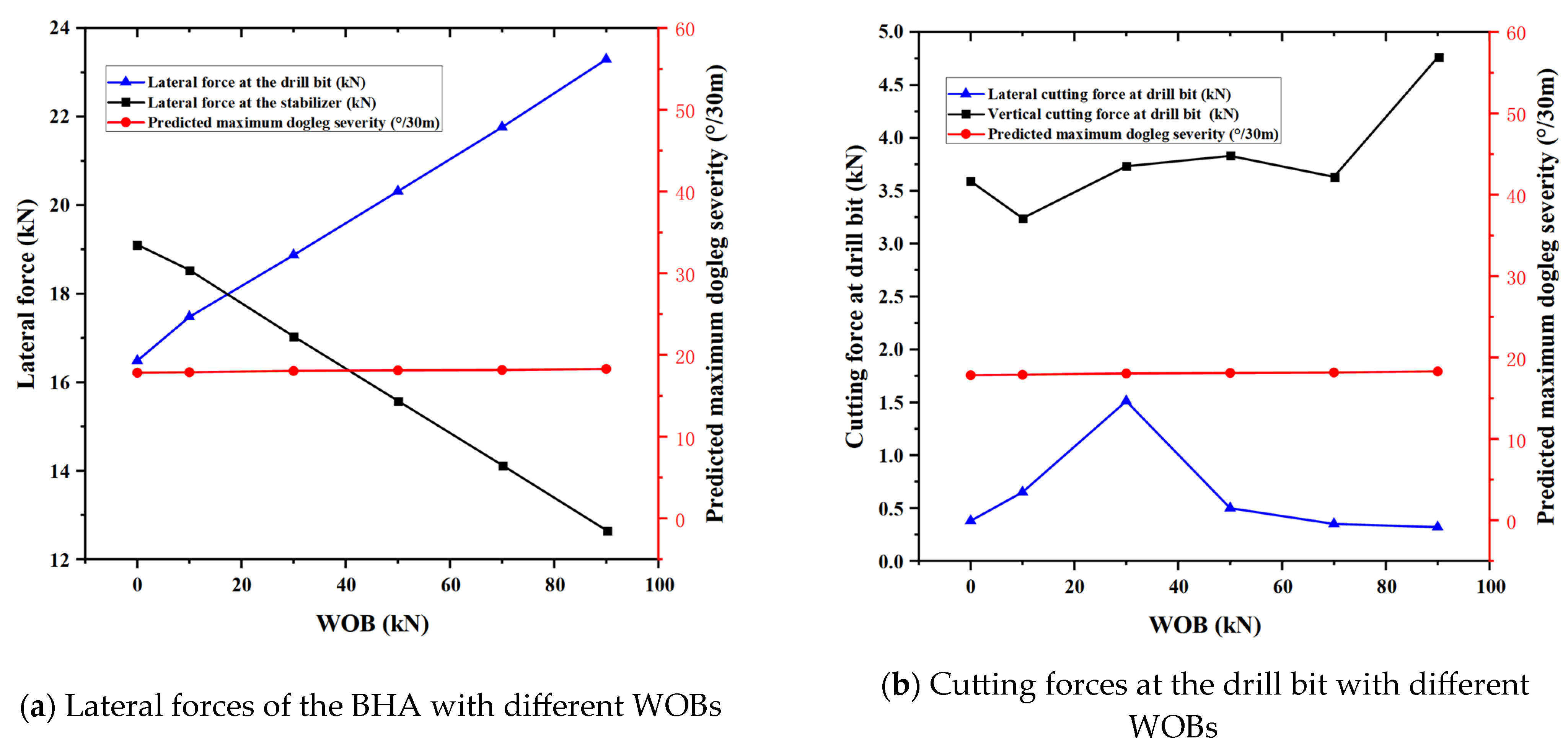
5.4. Analysis of the Effects of WOB and Pump Displacement on the Drilling Tool Assemblies

The tool face turning angle of the screw drilling tool was taken as 2.5°, the stratigraphic nature was selected as siltstone mudstone (modulus of elasticity 1 × 10⁴ MPa, Poisson’s ratio 0.30), and the drill bit position was located at 1550 m of the borehole trajectory; the bit rotational speed was 80 rpm, pump displacement was 3.6 m³/min, and bit torque was 20 kN·m. The WOB of the drilling tools was incremented from 0 kN to 90 kN, and the dynamics of the bottom drilling tool combination were calculated to evaluate the changes in parameters such as lateral force of the drilling tools, as shown in

Table 7. Calculation results of BHA under different WOB values.

WOB (kN)	0	10	30	50	70	90
Maximum stress (bending stress) (MPa)	1.09	2.16	1.76	1.00	2.05	1.44
Lateral cutting force at drill bit (kN)	0.38	0.65	1.51	0.50	0.35	0.32
Vertical cutting force at drill bit (kN)	3.59	3.24	3.73	3.83	3.63	4.76
Lateral force at drill bit (kN)	16.485	17.474	18.869	20.312	21.760	23.291
Lateral force at the stabilizer (kN)	19.108	18.537	17.034	15.578	14.127	12.656
Predicted maximum degree of dogleg (°/30 m)	17.824	17.873	18.035	18.104	18.164	18.292

and Figure 10.

The results show that, when the tool face angle is 2.5°, as the bottom-hole weight on bit (WOB) gradually increases, the lateral force at the bit significantly increases, while the lateral force at the stabilizer gradually decreases. The vertical and lateral cutting forces at the bit change but do not increase or decrease linearly; notably, when the WOB is 30 kN, both the vertical and lateral cutting forces reach a maximum value. The ultimate build-up rate is insensitive to changes in WOB and only increases slightly.

With a tool face angle of 2.5°, a bottom-hole weight on bit (WOB) of 30 kN, and other parameters unchanged, the pump displacement was varied. The calculation results are shown in

Table 8. Calculation results of BHA under different pump displacement values.

Pump Displacement (m3/min)	3.2	3.4	3.6	3.8	4.0	4.2
Maximum stress (bending stress) (MPa)	1.98	2.05	1.64	1.76	1.69	1.47
Lateral cutting force at drill bit (kN)	1.38	1.49	1.57	1.51	1.23	0.86
Vertical cutting force at drill bit (kN)	3.66	3.67	3.75	3.73	3.74	3.76
Lateral force at drill bit (kN)	18.640	18.712	18.788	18.869	18.953	19.052
Lateral force at the stabilizer (kN)	17.302	17.218	17.128	17.034	16.934	16.843
Predicted maximum degree of dogleg (°/30 m)	18.004	18.014	18.024	18.035	18.048	18.077

and Figure 11 below. The calculations indicate that changing the pump displacement has minimal effect on the ultimate build-up rate. However, pump displacement alters the performance of the positive displacement motor (PDM) and influences the forces on the BHA and the bit cutting forces. As the pump displacement increases, the lateral force at the stabilizer decreases, while the lateral force at the bit increases. The vertical and lateral cutting forces at the bottom hole vary with pump displacement but do not exhibit linear increases or decreases; when the pump displacement is 3.6 m³/min, both the vertical and lateral cutting forces reach maximum values.

Further calculations indicate that the bit rotational speed and rate of penetration (ROP) have minimal impact on the lateral force of the BHA as well as on the build-up rate. This is because the bit rotation speed does not significantly alter the forces and deformations of the BHA; similarly, the ROP does not directly change the BHA’s force–deformation state, but only modifies the tool’s position in the wellbore and the constraint conditions imposed by the borehole.

5.5. Analysis of Model Algorithm Advancements and Limitations

Advancements in Methodology:

(1).

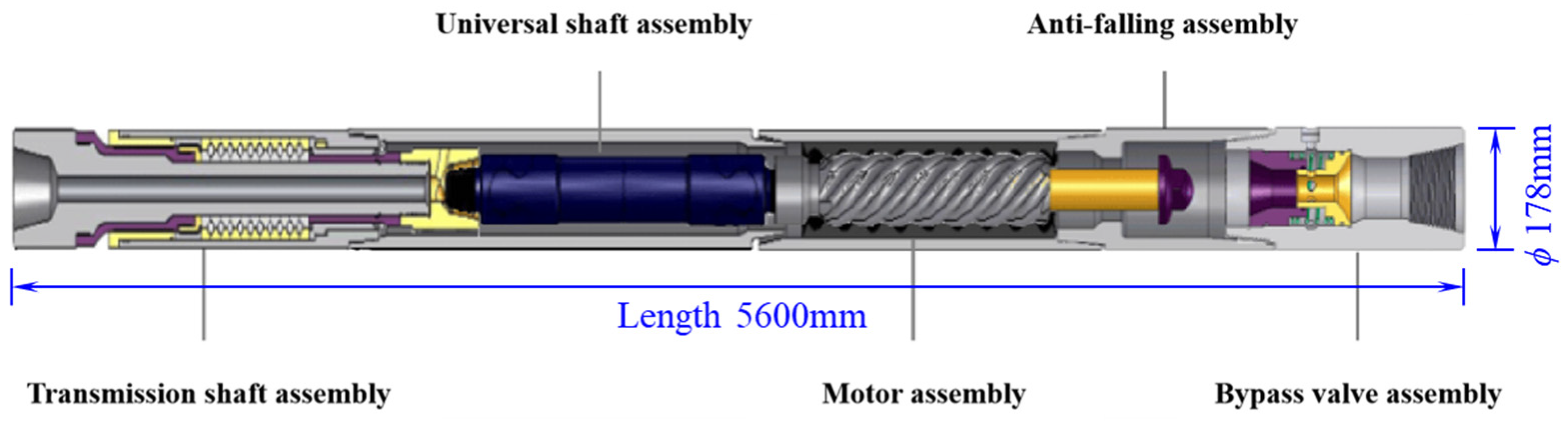
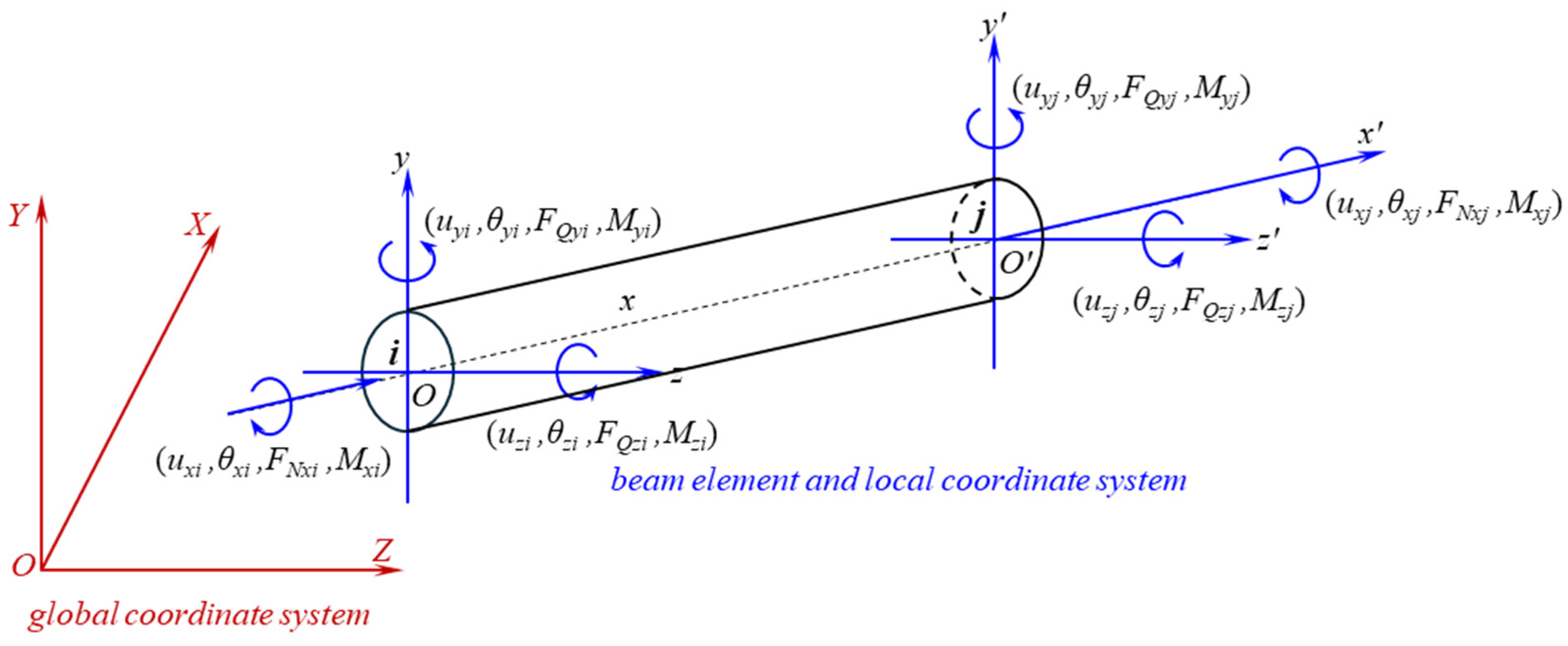
Transient dynamics modeling: This study establishes a transient dynamic computational model for deflection tools driven by positive displacement motors (PDMs). The model employs a spatial frame finite element formulation based on Euler–Bernoulli beam theory, simultaneously characterizing deformation and motion across six degrees of freedom (axial, transverse [x,y], and torsional) at each drill string node.

(2).

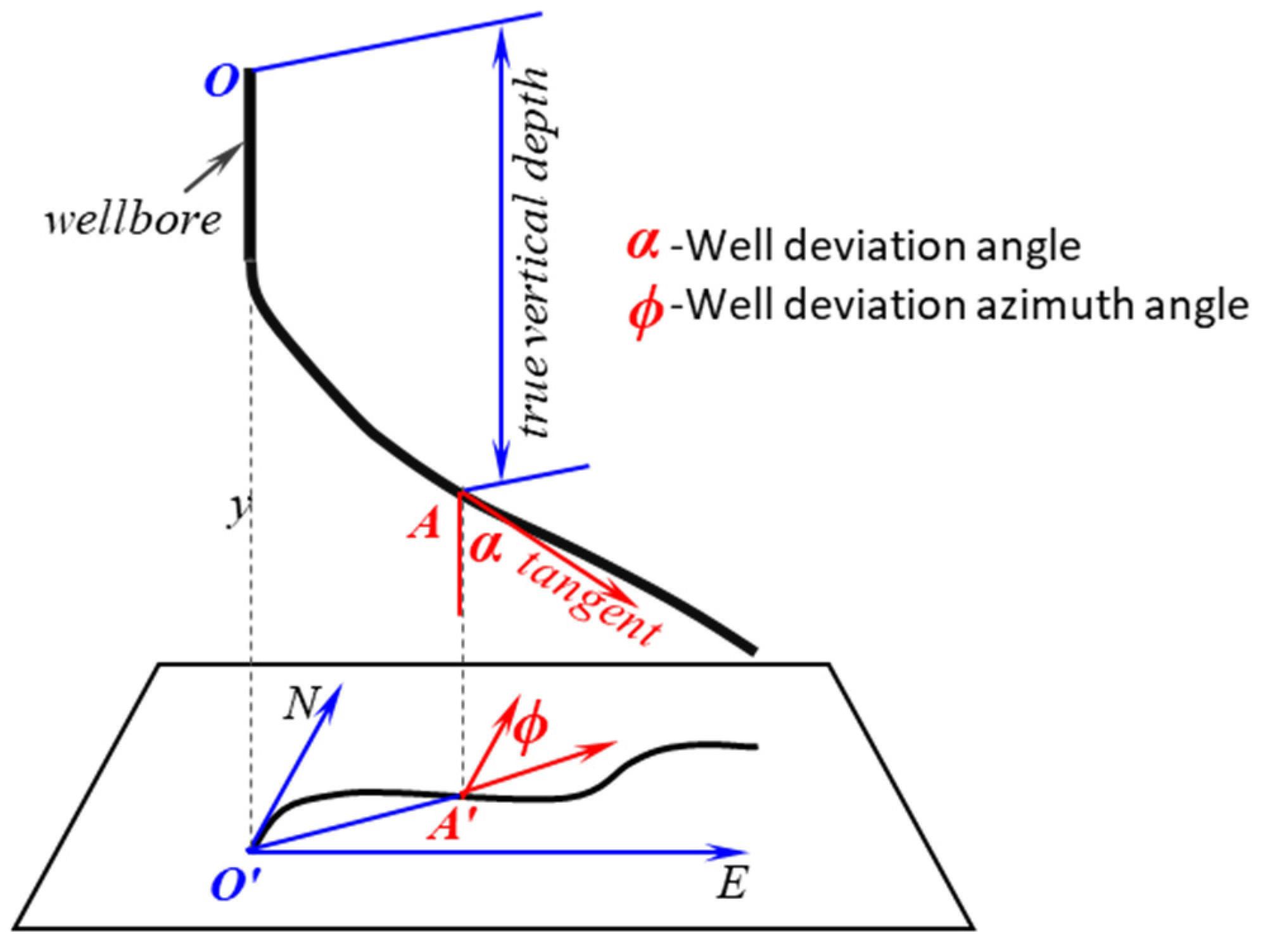
Trajectory-adaptive computation: The methodology meticulously accounts for directional well trajectory effects through three-dimensional coordinate transformations that quantify tool deviation from the wellbore centerline.

(3).

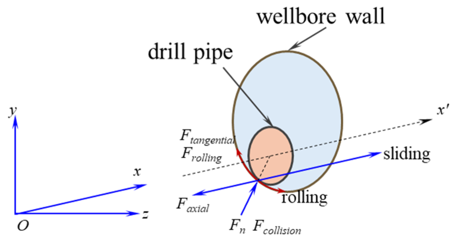
Advanced pipe–soil interactions: Incorporating axial/tangential friction, normal contact forces, and collision reactions between the drill string and unconsolidated formation, the model integrates pipe–soil dynamics with a p-y curve methodology. This establishes a geometric correlation between the penetration depth and contact area, significantly enhancing contact force calculation accuracy in soft formations.

(4).

Computational optimization: The algorithm implements a temporally discrete dynamic scheme, solving large-scale sparse equation systems via the GMRES method with iLU preconditioning, thereby improving computational efficiency compared to conventional solvers.

Due to the inherent complexity of mechanical analysis for drill strings and BHAs in shallow soft subsea formations, several factors were neglected in the present methodology and case studies:

(1).

Bit motion simplification: The transient displacement of the bit in all directions was modeled solely as a combination of harmonic and random components. Future work should couple the bit’s equations of motion with the BHA dynamics to capture interaction effects.

(2).

Formation heterogeneity: Shallow subsea strata typically comprise interbedded sandy and muddy lithologies, exhibiting increasing strength with depth. For improved accuracy, layer-specific p-y curve analyses should be implemented for distinct geological horizons along the burial depth profile.

(3).

Sand liquefaction potential: Continuous vibrations during drilling in water-saturated sandy formations may induce soil liquefaction, significantly reducing lateral support for steerable assemblies. This mechanism warrants dedicated experimental and numerical investigations.

(4).

Wellbore irregularities: The effects of borehole wall collapse (“cavings”), washouts, shale creep-induced narrowing, and cuttings beds in horizontal sections were not considered. Subsequent research should quantify the tool–wall contact area and indentation depth in irregular wellbores and develop advanced models for contact force prediction under realistic geometric constraints.

Additionally, computational methods associated with the numerical algorithms of the model itself should be investigated, including more efficient time-domain discrete iterative algorithms and high-accuracy solvers for large-scale equation systems.

6. Conclusions and Suggestions

(1) A mechanical calculation method for the BHA based on three-dimensional finite element and transient dynamics analysis is proposed. By introducing the pipe–soil dynamics and the p-y curve method, and considering the axial and tangential frictional forces, normal reaction force, and collision reaction force between the drill string and the soft borehole wall, the calculation of the contact reaction force between the drilling tool and the soft formation was improved. The dynamic discrete algorithm in the time domain and the efficient solution algorithm for large systems of equations were optimally selected, achieving the quantitative characterization of the deformation, force-bearing, and vibration drilling of the BHA in the shallow and soft seabed formation.

(2) The case analysis shows that, as the tool face rotation angle increases, the lateral forces at the bit and the stabilizer increase significantly, and the predicted maximum dogleg severity within the first 10 m in front of the bit gradually increases. When the tool face rotation angle exceeds 2.5°, the predicted maximum dogleg severity near the bit reaches 18.024°/30 m. As the WOB value gradually increases, the maximum stress on the drilling tool is the bending stress, and its value gradually decreases; the maximum lateral cutting force gradually decreases, and the maximum vertical cutting force gradually increases; the lateral force at the bit gradually increases, and the lateral force at the stabilizer gradually decreases; the predicted maximum dogleg severity within the first 10 m in front of the bit increases slightly.

(3) It is recommended to conduct multi-objective optimization research on drilling engineering parameters for directional drilling in shallow soft seabed formations. Key optimization objectives should include borehole quality, drilling safety, the rate of penetration (ROP)/drilling efficiency, and drilling cost. Optimizable parameters encompass mechanical parameters (WOB, rotational speed), hydraulic parameters (pump pressure, flow rate), drilling fluid properties (density, viscosity), and directional parameters (tool face angle, build-up rate). Particularly for directional drilling in shallow unconsolidated seabed formations, hydraulic and directional parameters constitute the critical variables directly governing wellbore stability and directional performance. The recommended multi-objective optimization algorithms include Response Surface Methodology (RSM), intelligent optimization algorithms (e.g., NSGA-II), and multi-criteria decision-making methods.

(4) Given that this study primarily focuses on numerical computational models and solution algorithms, less attention was paid to experimental testing and analysis of influencing factors. The following research avenues are recommended for future work: (a) Conduct simulated experiments on BHA deflection drilling in shallow soft seabed formations, measuring dynamic lateral forces at stabilizers, deflection tool support arms, and drill bits to accumulate reliable validation data for theoretical methods. (b) Investigate the impact of irregular wellbores and wellbore collapse in shallow soft formations on deflection drilling performance. (c) Assess vibration-induced risks of soil liquefaction in shallow soft seabed strata during drilling operations and evaluate subsequent effects of liquefied surrounding formations on deflection drilling. (d) Develop a near-bit measurement sub- and integrated data acquisition/transmission/analysis system tailored for directional drilling in shallow soft seabed formations. This enables the real-time monitoring of critical parameters during build-up drilling in unconsolidated strata, including transient lateral forces, bending strains, and triaxial vibration accelerations at key BHA locations. (e) Synergize the predictive algorithms presented in this study with experimental data and near-bit measurements. Employ optimized machine learning methods to enhance the prediction accuracy of directional drilling parameters—inclination, azimuth, and lateral forces—in shallow soft formations. And implement adaptive real-time control through BHA-mounted steering subs based on these predictions.

References

1. Sampaio, J.H., Jr. Designing three-dimensional directional well trajectories using Bézier curves. J. Energy Resour. Technol. 2017, 139, 032901. [Google Scholar] [CrossRef]
2. Di, Q.F.; Peng, G.R. The study of the influence of well trajectory parameters on side force acting on bit. J. Xi’an Pet. Inst. (Nat. Sci. Ed.) 2000, 15, 20–23. [Google Scholar] [CrossRef]
3. Di, Q.F.; Zhu, W.P.; Yao, J.L.; Zou, H. Dynamic model of bottom hole assembly used in pre-bending dynamic vertical and fast drilling technology. Acta Pet. Sin. 2007, 28, 118–121. [Google Scholar] [CrossRef]
4. Abbassian, F.; Dunayevsky, V. Application of stability approach to torsional and lateral bit dynamics. SPE Drill. Complet. 1998, 13, 99–107. [Google Scholar] [CrossRef]
5. Greenwood, J.A. Directional control and rathole elimination while underreaming depleted formations with a rotary-steerable system. SPE Drill. Complet. 2018, 33, 252–258. [Google Scholar] [CrossRef]
6. Epikhin, A.; Zhironkin, V.; Cehlar, M. Prospects for the use of technology of rotary steerable systems for the directional drilling. In Proceedings of the E3S Web of Conferences, Constanta, Romania, 26–27 June 2020; EDP Sciences: Les Ulis, France, 2020; Volume 174, p. 01022. [Google Scholar] [CrossRef]
7. Liu, H.S.; Ma, T.S.; Chen, P.; Wang, X.D.; Wang, X.M. Mechanical behaviors of bottom hole assembly with bent-housing positive displacement motor under rotary drilling. Arab. J. Sci. Eng. 2018, 44, 6029–6043. [Google Scholar] [CrossRef]
8. Chen, R.; Huang, W.J.; Gao, D.L. Prediction model of build-up rate for bottom-hole assembly in rotary drilling. Geoenergy Sci. Eng. 2025, 246, 213610. [Google Scholar] [CrossRef]
9. Yu, T.; Li, X.Y.; Zhang, H.B.; Duan, C.C.; Zeng, H.; Agila, W. Nonlinear analysis of axial-torsional vibration of drill string based on a 3 DOF model. Adv. Mech. Eng. 2022, 14, 1–17. [Google Scholar] [CrossRef]
10. Yang, C.X.; Wang, R.H.; Han, L.J.; Xue, Q.L. Dynamic analysis of the longitudinal vibration on bottom drilling tools. J. Vibroeng. 2020, 22, 252–266. [Google Scholar] [CrossRef]
11. Mohammad, M.J.; Shiri, H.; Martins, C.A. Numerical investigation of the nonlinear drill string dynamics under stick–slip vibration. Vibration 2024, 7, 1086–1110. [Google Scholar] [CrossRef]
12. Guo, Y.C.; Pang, X.Q.; Li, Z.X.; Guo, F.T.; Song, L.C. The critical buoyancy threshold for tight sandstone gas entrapment: Physical simulation, interpretation, and implications to the Upper Paleozoic Ordos Basin. J. Pet. Sci. Eng. 2017, 149, 88–97. [Google Scholar] [CrossRef]
13. Li, W.; Huang, G.L.; Ni, H.J.; Yu, F.; Huang, B.; Jiang, W. Experimental study and mechanism analysis of the motion states of bottom hole assembly during rotary drilling. J. Pet. Sci. Eng. 2020, 195, 107859. [Google Scholar] [CrossRef]
14. Zhu, X.H.; Li, K.; Li, W.Z. Drill string mechanical behaviors of large-size borehole in the upper section of a 10000 m deep well. Nat. Gas Ind. 2024, 44, 49–57. [Google Scholar] [CrossRef]
15. Akgun, F. A finite element model for analyzing horizontal well BHA behavior. J. Pet. Sci. Eng. 2004, 42, 121–132. [Google Scholar] [CrossRef]
16. Li, H.; Zhang, P.; Ma, C.; Zhao, J.; Shi, Y.; Jiang, X.B.; Yu, J.S. Optimization of lateral force balance of PDC bits based on ant colony particle swarm hybrid algorithm. Drill. Prod. Technol. 2009, 32, 58–60. [Google Scholar] [CrossRef]
17. Wang, Z.B.; Yang, H.Y.; Wang, W.C.; Chen, F.; Di, Q.F. Prediction method of combined guiding force of pre-bent BHA bit based on PSO-SVR algorithm. J. Shanghai Univ. (Nat. Sci. Ed.) 2024, 30, 968–979. [Google Scholar] [CrossRef]
18. Oueslati, H.; Jain, R.; Reckmann, H.; Ledgerwood, L.I.; Pessier, R.; Chandrasekaran, S. New insights into drilling dynamics through high-frequency vibration measurement and modeling. In Proceedings of the SPE Annual Technical Conference and Exhibition, New Orleans, LA, USA, 30 September–2 October 2013; SPE: Richardson, TX, USA, 2013; p. D031S042R001. [Google Scholar] [CrossRef]
19. Wang, P.; Tang, B.; Ji, J.Y.; Feng, D. A new method for mechanical calculation of bottom hole assembly in rotary steerable system. Chin. Q. Mech. 2022, 43, 670–680. [Google Scholar] [CrossRef]
20. Hai, W.G.; Xue, Q.L.; Wang, M.C.; He, Y.M. Parameter optimization based on deepwater drilling system simulation: A pre-salt exploration well in Brazil. Geoenergy Sci. Eng. 2024, 241, 213120. [Google Scholar] [CrossRef]
21. Chen, Y.; Gao, Y.H.; Chen, L.T.; Wang, X.R.; Liu, K.; Sun, B.J. Experimental investigation of the behavior of methane gas hydrates during depressurization-assisted CO2 replacement. J. Nat. Gas Sci. Eng. 2019, 61, 284–292. [Google Scholar] [CrossRef]
22. Fang, P.; Yang, K.; Li, G.; Feng, Q.F.; Ding, S.J. Vibration-collision mechanism of dual-stabilizer bottom hole assembly system in vertical wellbore trajectory. J. Vibroeng. 2023, 25, 226–246. [Google Scholar] [CrossRef]
23. Gao, D.L.; Wang, Y.B. Some research progress in deepwater drilling mechanics and control technology. Acta Pet. Sin. 2019, 40, 102. [Google Scholar] [CrossRef]
24. Chen, W.; Shen, Y.L.; Chen, R.B.; Zhang, Z.X.; Rawlins, S. Simulating drill-string post-buckling state and weight transfer with advanced transient dynamics model. In Proceedings of the IADC/SPE International Drilling Conference and Exhibition, Galveston, TX, USA, 3–5 March 2020. SPE-199557-MS. [Google Scholar] [CrossRef]
25. American Petroleum Institute. Planning, Designing, and Constructing Fixed Offshore Platforms-Working Stress Design, 22nd Edition. API. 2020, API RP 2A-WSD-2014(2020). Available online: https://www.intertekinform.com/en-au/standards/api-rp-2a-wsd-2014-r2020--98372_saig_api_api_2925841/?srsltid=AfmBOor1dn_YM_Y41tASmJ837JcNAD22Uz4xOwp3Psa1TT2Xz-G4oejo (accessed on 16 June 2025).
Figure 1. Deflecting tool for directional wells in deepwater shallow layers.
Processes 13 01947 g001
Figure 2. Global and local coordinate systems of the BHA beam element.
Processes 13 01947 g002
Figure 3. Well deviation angle and deviation azimuth angle.
Processes 13 01947 g003
Figure 4. Contact, friction, and collision between drill string and wellbore wall.
Processes 13 01947 g004
Figure 5. Geometric model of the contact area between the drill pipe and wellbore wall.
Processes 13 01947 g005
Figure 6. Overview of the case.
Processes 13 01947 g006
Figure 7. The contact positions of the BHA at the wellbore bottom hole under different tool face rotation angles.
Processes 13 01947 g007
Figure 8. Stress distribution of the BHA during inclined drilling.
Processes 13 01947 g008
Figure 9. Lateral force and predicted maximum dogleg severity of the BHA under different tool face rotation angles.
Processes 13 01947 g009
Figure 10. Lateral force and cutting force of the BHA under different values of WOB.
Processes 13 01947 g010
Figure 11. Lateral force andCutting force of the BHA under different values of pump displacement.
Processes 13 01947 g011