Research on an Automated Cleansing and Function Fitting Method for Well Logging and Drilling Data

Abstract

Oilfield data is characterized by complex types, large volumes, and significant noise interference, so data cleansing has become a key procedure for improving data quality. However, the traditional data cleansing process needs to deal with multiple types of problems, such as outliers, duplicate data, and missing values in turn, and the processing steps are complex and inefficient. Therefore, an integrated data cleansing and function fitting method is established. The fine-mesh data density analysis method is utilized to cleanse outliers and duplicate data, and the automated segmented fitting method is used for missing data imputation. For the real-time data generated during drilling or well logging, data cleansing is realized through grid partitioning and data density analysis, and the cleansing ratio is controlled by data density threshold and grid spacing. After data cleansing, based on similar standards, the cleansed data is segmented, and the fitting function type of each segment is determined to fill in the missing data, and data outputs with any frequency can be obtained. For the analysis of the hook load data measured by sensors at the drilling site and obtained from rig floor monitors or remote centers, the data cleansing percentage reaches 98.88% after two-stage cleansing, which still retains the original trend of the data. After data cleansing, the cleansed data are modeled through the automated segmented fitting method, with Mean Absolute Percentage Errors (MAPEs) less than 3.66% and coefficient of determination (R²) values greater than 0.94. Through the integrated data processing mechanism, the workflow can synchronously eliminate outliers and redundant data and fill in the missing values, thereby dynamically adapting to the data requirements of numerical simulation and intelligent analysis and significantly improving the efficiency of on-site data processing and decision-making reliability in the oilfield.

1. Introduction

There is a huge amount of data in the oilfield, including all types of basic raw data generated during the processes of exploration and development, engineering operations, and business management. These data are generated in real time at the oilfield and form the basis for exploration and development deployment, comprehensive analysis, and management decision-making in the oilfield.

Due to reasons such as sensor faults, transmission constraints, manual input errors, and abnormal events, there is a lot of noise in various types of data generated in the oilfield. The unprocessed data increase the workload of subsequent analysis, which is very likely to cover up the value of the data. During data cleansing processes, information such as anomalies and duplicates can be deleted, and missing values can be supplemented according to data trends. The data quality is effectively improved to provide valuable and logical input data for subsequent simulation calculations and intelligent models, thereby reducing the barriers impeding real-time analysis and decision-making.

Data cleansing is an effective means to improve data quality, and solve problems faced in data cleansing mainly include missing values, similar duplicates, anomalies, logical errors, and inconsistent data [1]. Different cleansing methods need to be selected and applied to solve different data quality problems effectively.

For missing data problems, discarding data is the simplest method. However, when the proportion of missing data is high, this method may lead to the deviation of data distribution, which affects the derivation of the accurate conclusion of the research problem. It is usually necessary to choose an appropriate method to fill in the missing data [2,3,4]. Wu et al. (2012) proposed a missing data filling method based on incomplete data clustering analysis that calculates the overall dissimilarity degree of incomplete data by defining dataset variance with constrained tolerance and applies incomplete data clustering results to fill in the missing data [2]. de A. Silva and Hruschka (2009) proposed an evolutionary algorithm for filling in missing data, discussed the impact of data filling on classification results, and demonstrated that classification results obtained after applying the method to fill in the data were less biased through the application of bioinformatics datasets [3]. Antariksa et al. (2023) presented a novel well logging data imputation method based on the comparison of several time-series deep learning models. They compared long short-term memory (LSTM), gated recurrent unit (GRU), and bidirectional LSTM (Bi-LSTM) models using the well dataset for the West Natuna Basin in Indonesia, concluding that the LSTM performed best with the highest R² values and the lowest Root Mean Squared Errors (RMSEs) [4].

In order to solve the problem of data redundancy with duplicate or highly similar records in the data storage system, the Sorted Neighborhood Method (SNM) is a common method for identifying similar duplicate records [5,6]. When using the SNM algorithm, all data records in the dataset need to be compared, and the time complexity is high. Zhang et al. (2010) analyzed the defects of the SNM algorithm and pointed out that window size selection and keyword sorting are key processes that impact matching efficiency and accuracy. They proposed an optimized algorithm based on SNM, which processed more than 2000 literature records by using methods of keyword sorting through preprocessing, the multiple proximity sorting of different keywords, and window scalability. They compared traditional and optimized algorithms, showing that the optimized algorithm has obvious advantages in recall rate and execution time [5]. Li et al. (2021) proposed an optimized algorithm based on the random forest and adaptive window methods. Different from the traditional SNM algorithm, the algorithm uses the random forest method to form a subset containing representative features and reduces the comparison time between data records through dynamic adaptive windows. They conducted experiments to demonstrate that the proposed method performs better than the traditional method [6].

For abnormal data that highly deviate from expectations and do not conform to statistical laws due to environmental or human factors, the discrimination methods include the physical discrimination method, the statistical discrimination method [7], and the machine learning method [8,9,10]. The physical discrimination method refers to the identification of outliers based on objective understanding and timely elimination. For the statistical discrimination method, Hou (2024) analyzed three discrimination criteria, including the Raida criterion, the Grubbs criterion, and the Dixon criterion, and compared the applicable conditions of the three criteria through example calculations. It was pointed out that when the outlier discrimination requirements are rigorous, multiple criteria can be used for determination at the same time [7]. Gao et al. (2011) analyzed the shortcomings of the Local Outlier Factor method. Based on the framework of the LOF method, the shortcomings of the traditional method were remedied through variable kernel density estimation and weighted neighborhood density estimation, thereby improving the robustness of the parameter selection, which determines the local scope. The method was verified through multiple synthetic and real datasets, demonstrating that the method not only improves the outlier detection performance but is also easily applied to large datasets [8]. Banas et al. (2021) reviewed different methods for identifying and repairing bad well log data and proposed an iterative and automated routine based on the Multiple Linear Regression (MLR) method to identify outliers and repair well log curves. The proposed workflow illustrated the data processing efficiency without compromising accuracy [9]. Gerges et al. (2022) built an interactive data quality control and preprocessing lab. They provided local outlier factor (LOF), one-class support vector machine (SVM), and isolation forest (IF) algorithms for users to detect and remove outliers in well log and core datasets. Through testing, they observed that more than 80% of the processed data could be directly used in the subsequent petrophysical workflows without further human editing [10].

For data with logical errors, Fellegi and Holt (1976) proposed a strict formalized mathematical model, the Fellegi–Holt model, which defines constraint rules according to the domain knowledge, applies mathematical methods to obtain closed sets with rules, and, for each record, automatically determines whether the rule has been violated [11]. Chen et al. (2005) analyzed the important role of professional knowledge in error data cleansing and proposed a cleansing method based on knowledge rules, which determines whether the data is wrong by defining knowledge rules in the rulebase. The proposed method is accurate and simple to use if users are familiar with the specific field and the knowledge rules of the data source are easy to obtain [12].

Common solutions to data inconsistencies across multiple data sources include sorting and fusion [13,14]. Motro et al. (2004) analyzed the shortcomings of sorting and fusion methods and proposed a solution by estimating the performance of data sources. By combining different features used to characterize performance of data sources and calculating a comprehensive evaluation value, the correct value is determined based on comprehensive evaluation [13]. Zhang et al. (2024) analyzed the traditional data repair method for inconsistencies based on the principle of minimal costs and pointed out that the repair scheme with minimal costs is usually incorrect, resulting in the low accuracy of the traditional method. They proposed a cleansing method for inconsistent data based on statistical reasoning, which uses the Bayesian network to infer the correctness probability of each repair scheme and selects the repair scheme with the highest probability as the optimal scheme, thereby improving the repair accuracy. They verified the method using synthetic and real datasets, demonstrating that the accuracy of the method is better than that of traditional repair methods [14].

In the process of modeling and analyzing time/depth series data, the trend term is often fitted with a single form of function [15,16]. Wu and Wang (2008) proposed a method to perform function fitting, assuming that the trending data is represented by a polynomial function. They optimized the order of the polynomial function based on statistical methods for error analysis. They processed the real-time projection data of composite materials to extract defect information effectively [15]. Al Gharbi et al. (2018) presented metaheuristics models to generate functional approximation equations that identify data trends. They proposed a functional approximator combining a sine function, a cosine function, and a polynomial with six parameters to be determined. Several metaheuristics approaches, including the greedy algorithm, the random algorithm, the hill climbing algorithm, and the simulated annealing algorithm, were utilized and compared. They obtained satisfactory fitting results using the simulated annealing algorithm, with a Mean Absolute Error (MAE) of 10.50 for drilling data [16].

In view of the data cleansing problem in the oilfield, the conventional data cleansing workflow is complicated, including procedures of statistical analysis, computerized methods, and manual steps. Common issues of outliers, missing values, and duplicates involve a variety of processing methods. According to data characteristics, data analysts need to select processing methods for each type of issue in sequence to achieve the complete data cleansing workflow. The data cleansing quality depends on the experience of data analysts and the understanding of data characteristics. In the data cleansing workflow, the lack of overall analysis of the oilfield data needs to be optimized. For the function fitting process after data cleansing, it is difficult to improve the fitting accuracy when assuming a single form of function to model data composed of segments that may follow different trends. Well logging and drilling data usually present significantly different trending characteristics depending on formation and drilling conditions. Therefore, it is more reasonable to perform segmented function fitting instead of adding complicated function terms in a global fitting function. The combined fitting function with more function types and more coefficients may cause solving complexity and overfitting problems. Al Gharbi et al. (2015) proposed a real-time automated data cleansing method based on statistical analysis that processes duplicate and abnormal information while retaining data trends [17]. On the basis, in this paper, the primary cleansing process is improved by optimizing the data density threshold. Based on similar criteria, the cleansed data are automatically divided into subsequences, and the fitting function of each subsequence is determined to achieve piecewise fitting. The automated cleansing and function fitting method of well logging and drilling data proposed in this paper can deal with outliers, duplicates, and missing values in an integrated manner, thereby significantly eliminating duplicate and abnormal information on the premise of retaining original data trends, automatically controlling the data frequency while guaranteeing data quality, and flexibly adapting to the input data requirements of subsequent simulation calculation and intelligent analysis.

2. Automated Data Cleansing and Function Fitting Method

In the petroleum field, a large amount of real-time data is generated in core processes such as geophysical exploration, drilling, logging, and production. A significant proportion of data are sequential data labeled by time or depth. The drilling process is a core procedure of petroleum engineering that refers to the systematic engineering of drilling wellbore holes underground using machinery or specialized technology to explore or exploit oil and natural gas. During the drilling process, a variety of critical data are measured in real time or in stages to monitor the drilling status, optimize operations, guarantee safety, and evaluate formation characteristics. Among all the data measured, well logging and drilling engineering data are two important types of data that help avoid drilling risks. Drilling engineering data, such as hook load, torque, and pump pressure, directly reflect downhole conditions, and well logging data help to identify formation changes, such as high-pressure layers and weak formations.

The method developed in this paper is applicable to well logging and drilling data. Well logging and drilling data are obtained through surface or downhole sensors and transmitted to rig floor monitors or remote centers during drilling or production at the oilfield site. Well logging data is obtained through sensors deployed into a well via cables or while-drilling tools. The data is transmitted back to the surface system for processing and interpretation and utilized to measure the physical properties of the formation and its fluids. Drilling engineering data is obtained through real-time monitoring, sensor measurements, logging techniques, and post-analysis. The data is mainly used to optimize drilling operations, guarantee safety, and evaluate formation characteristics.

The traditional data cleansing workflow is time consuming since outliers, duplicates, and missing values need to be processed using different methods separately, especially for large-scale datasets. The data cleansing quality and processing efficiency highly depend on the experience of data analysts and is hard to guarantee. Conventional function fitting approaches usually use a unique function globally and improve the fitting accuracy by increasing the function complexity. The complex fitting function with combined function types and a relatively large number of coefficients is not applicable for well logging or drilling data, which usually present significantly different trending characteristics in different segments. The integrated data processing workflow proposed in this paper can process outliers, duplicates, and missing values simultaneously and efficiently. The integrated workflow can be divided into two stages of data cleansing and function fitting. The data cleansing process deals with abnormal and duplicate data, while the function fitting process fills in missing data. The data cleansing method can efficiently cleanse the original data to achieve a very high cleansing percentage without losing trend descriptiveness through primary and secondary cleansing. The segmented function fitting method can determine the number of segments and the fitting function type of each segment based on data characteristics in an automated manner. Overall, the integrated workflow is automated and efficient, with minimal requirements regarding personnel experience and manual steps. Additionally, different stages of the workflow can be utilized independently based on different objectives of data application.

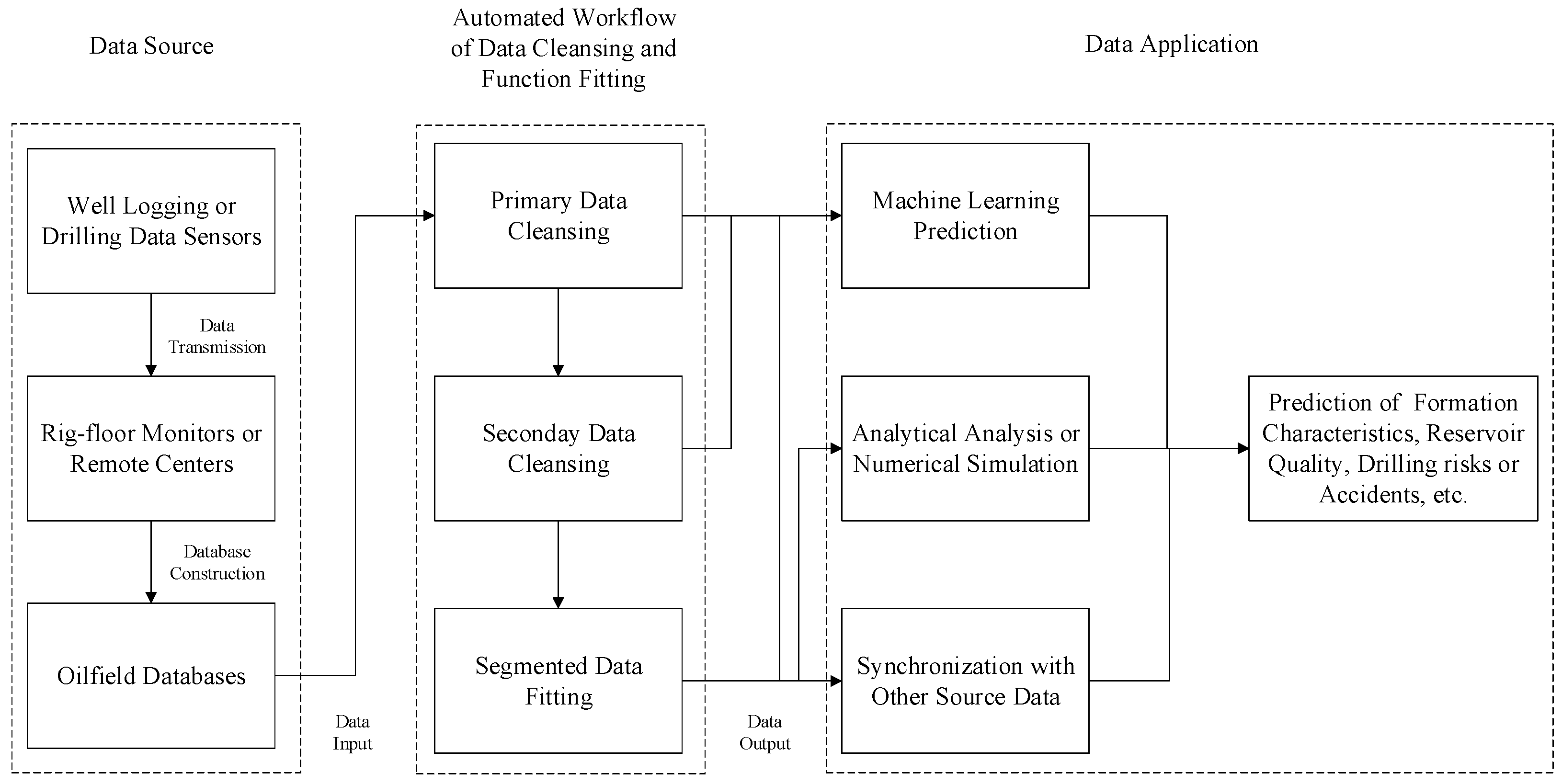
In the two-stage data cleansing workflow, the purpose of the primary cleansing process is to eliminate outliers and duplicate data, and the secondary cleansing process mainly aids in the function fitting process to obtain more accurate data trends and fill in the missing data. Therefore, only the primary cleansing process or the two-stage cleansing workflow can be selected for use depending on different objectives of data application. When the volume of the original data is very high and seriously exceeds the computational power of the subsequent analysis, or when the ultimate goal is to obtain data with a fixed frequency to be used as input for numerical simulation or to synchronize with data from other sources, the complete two-stage data cleansing workflow is necessary. However, when the original data volume is not very high and a certain percentage of slightly deviated data is acceptable, the primary cleansing process alone is satisfactory. The automated workflow for data cleansing and function fitting, along with the data source and application, is illustrated in Figure 1.

For the oilfield data that change with time or depth, the two-dimensional space composed of time/depth and the parameter is divided into subdomains based on horizontal and vertical division boundaries, and the data density distribution among subdomains is calculated. The primary cleansing of the data is implemented by optimizing the data density threshold and eliminating data in subdomains with data densities below the optimized threshold. On the basis of primary data cleansing, the time/depth dimension is partitioned, the median of the dataset is obtained at each time/depth interval, and other data in the interval are eliminated to achieve secondary cleansing. The cleansed data is fitted in segments to obtain parameter values at a specific time/depth, outputting parameters with a fixed frequency. The workflow of primary cleansing, secondary cleansing, and segmented function fitting is used to process multi-source parameter data in the oilfield to achieve data synchronization.

2.1. Primary Data Cleansing

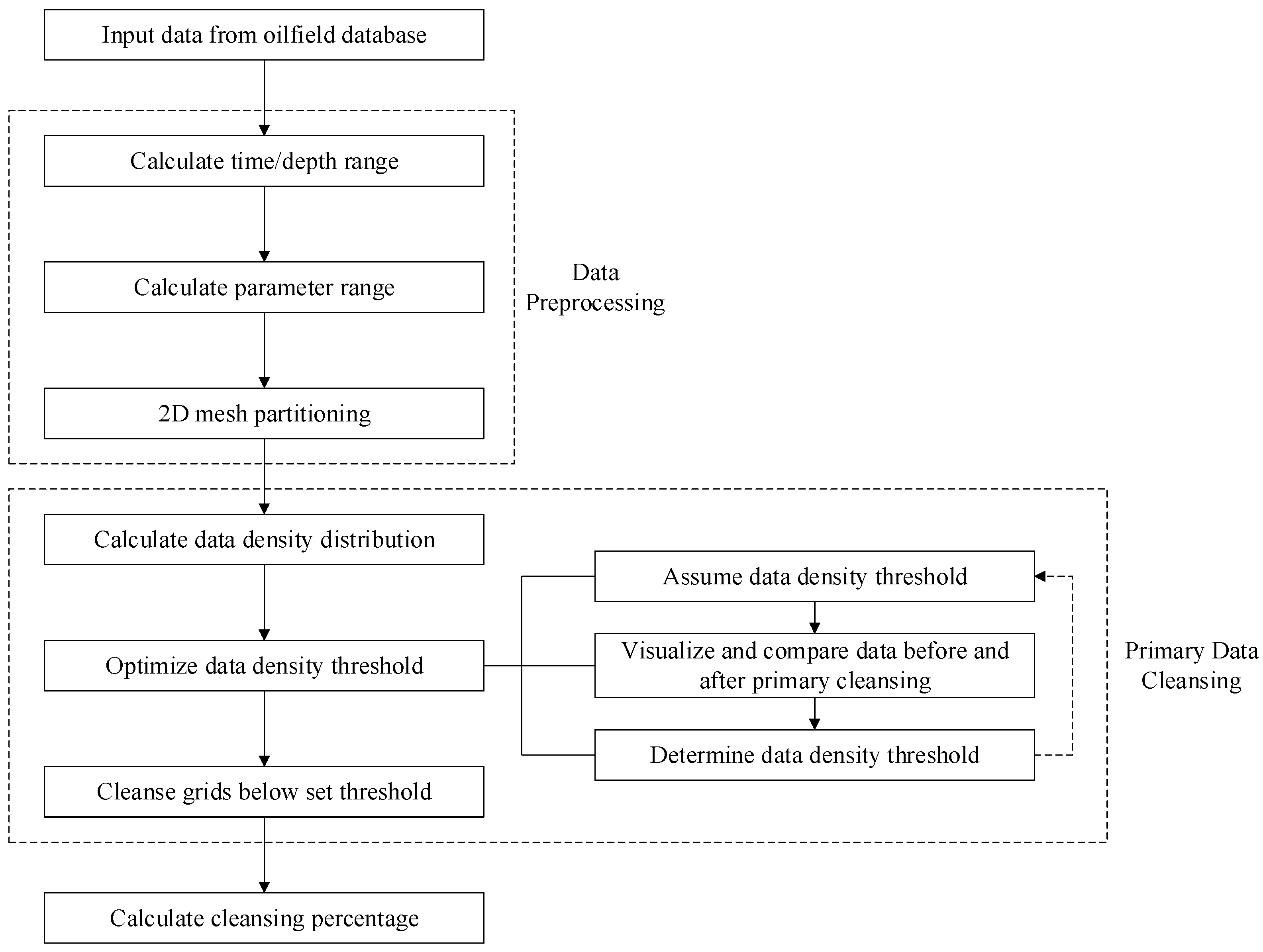
The purpose of the primary cleansing process is to eliminate outliers and duplicate data based on statistical data density analysis. The process of the primary data cleansing is illustrated in Figure 2.

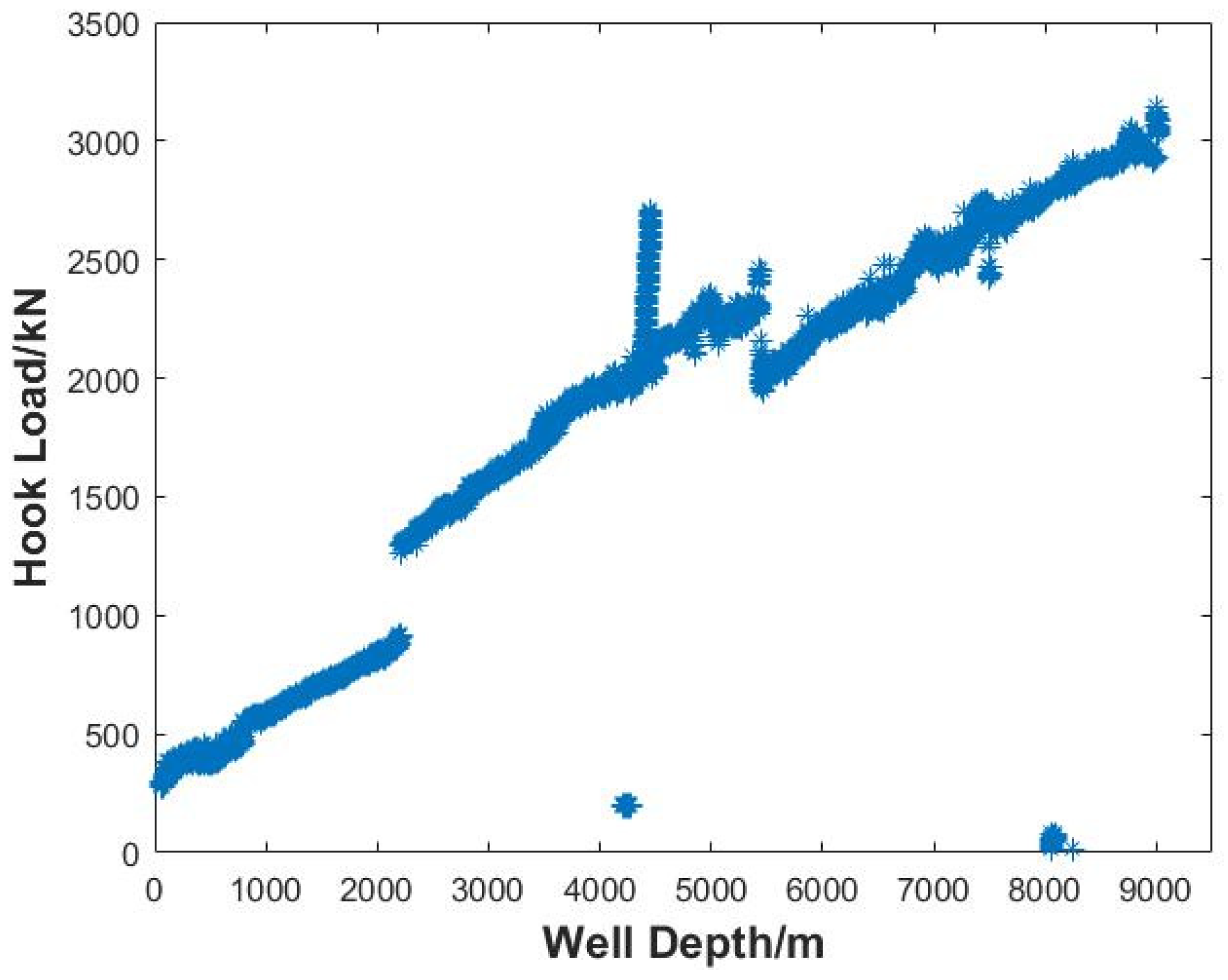
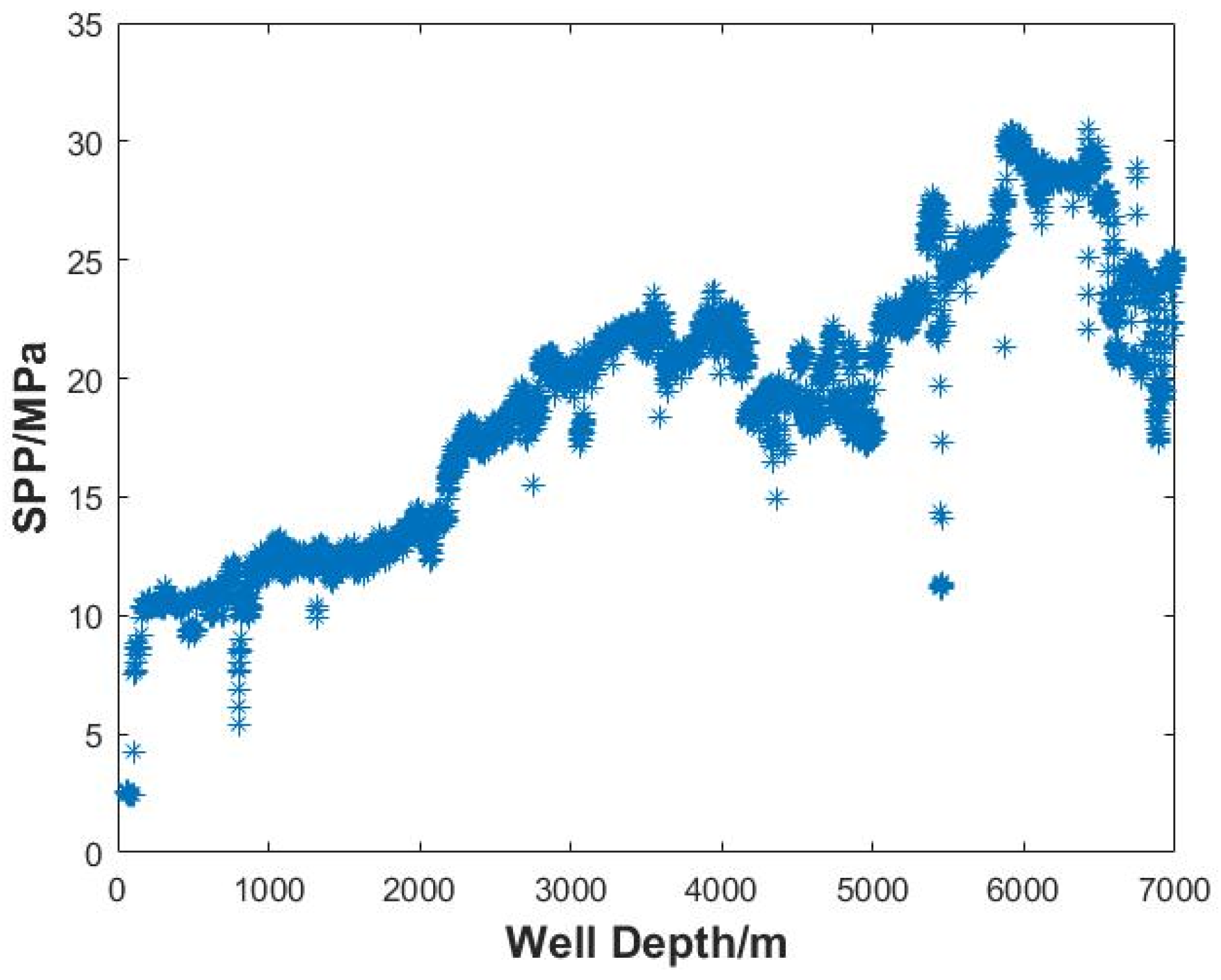
Firstly, data recorded at a specific time or depth interval from the oilfield site, such as well logging data, drilling engineering parameter data, etc., are collected. Based on any kind of parameter data collected, with time/depth on the horizontal axis and parameter on the vertical axis, a two-dimensional scatter plot is drawn, and the total amount of data before data cleansing is counted.

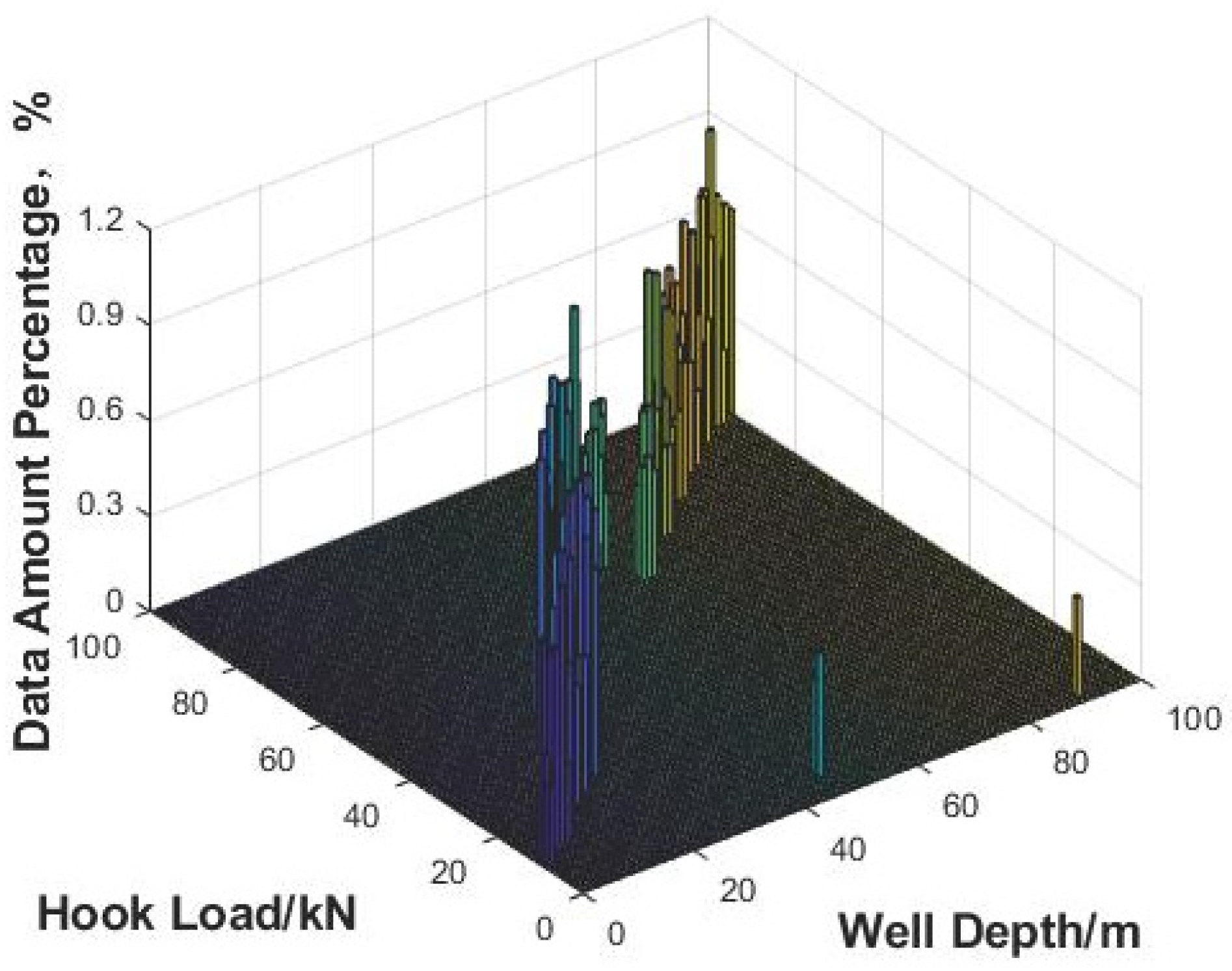
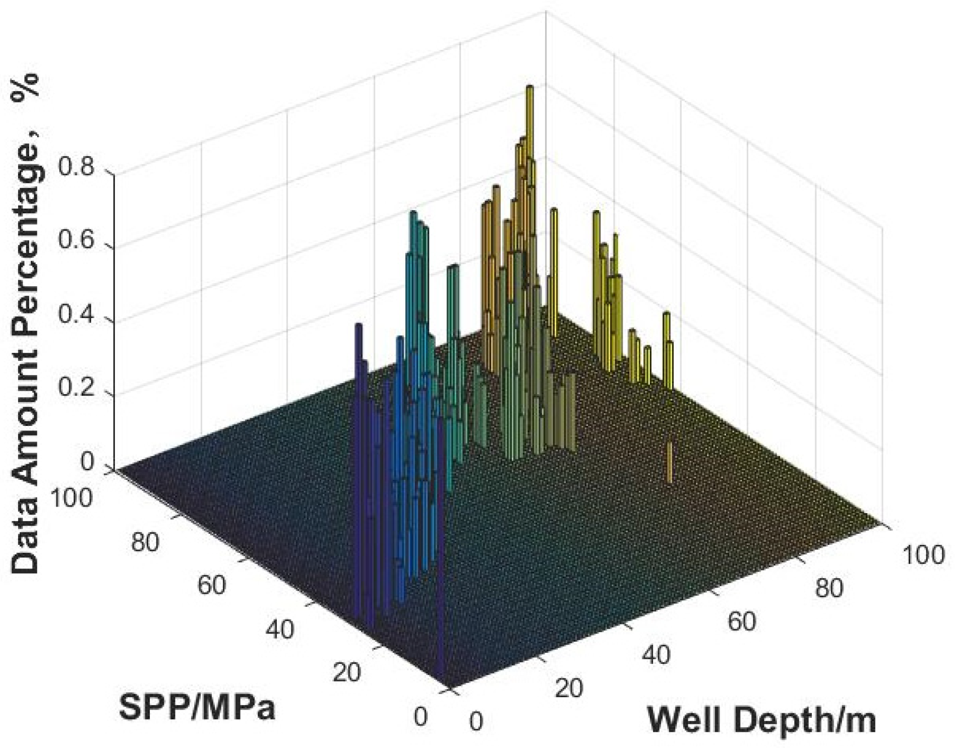
Secondly, based on the data before data cleansing, maximum and minimum values of the time/depth (abscissa) and that of the parameter (ordinate) are calculated to determine the value range of the data before cleansing. Taking the maximum and minimum values of the horizontal and vertical coordinates as the boundary, the partition interval or the number of partitions is set, and then the time/depth (abscissa) and the parameter (ordinate) are partitioned at equal intervals. The horizontal and vertical partition boundary lines are superimposed on the scatter map of the data before cleansing to form two-dimensional partition grids.

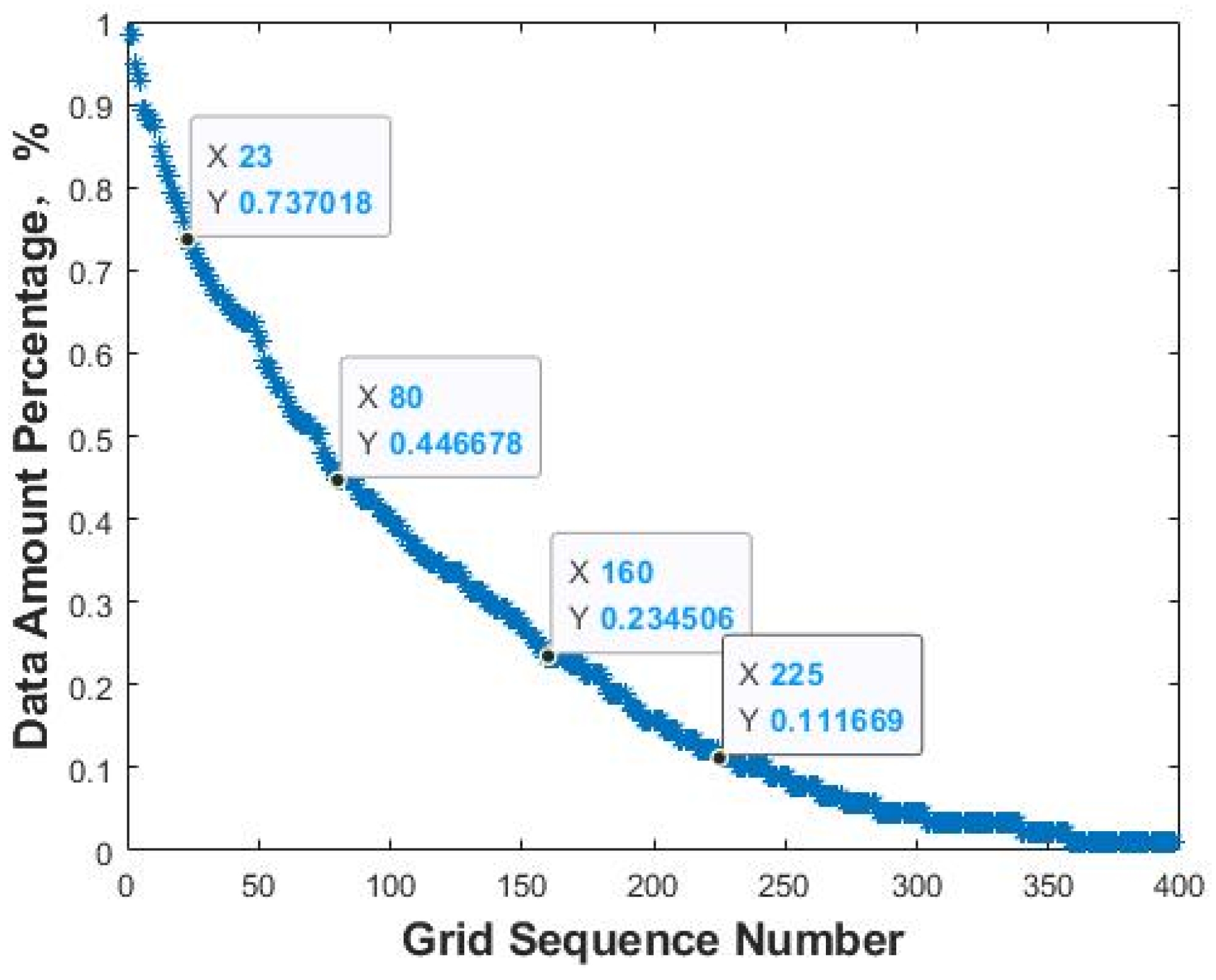
Thirdly, based on the two-dimensional grids on the plot, the amount of data in each grid is counted, and the percentage of data volume in each grid (data density) is calculated based on the total amount of data before data cleansing. The grids with data densities above 0 are sorted according to the value of the data density from large to small, and the grid sequence number is labeled. The data density curve is plotted with the grid sequence number as the abscissa and the data density as the ordinate. All inflection points are marked on the data density curve, and the data density values of the inflection points are assumed as the data density threshold.

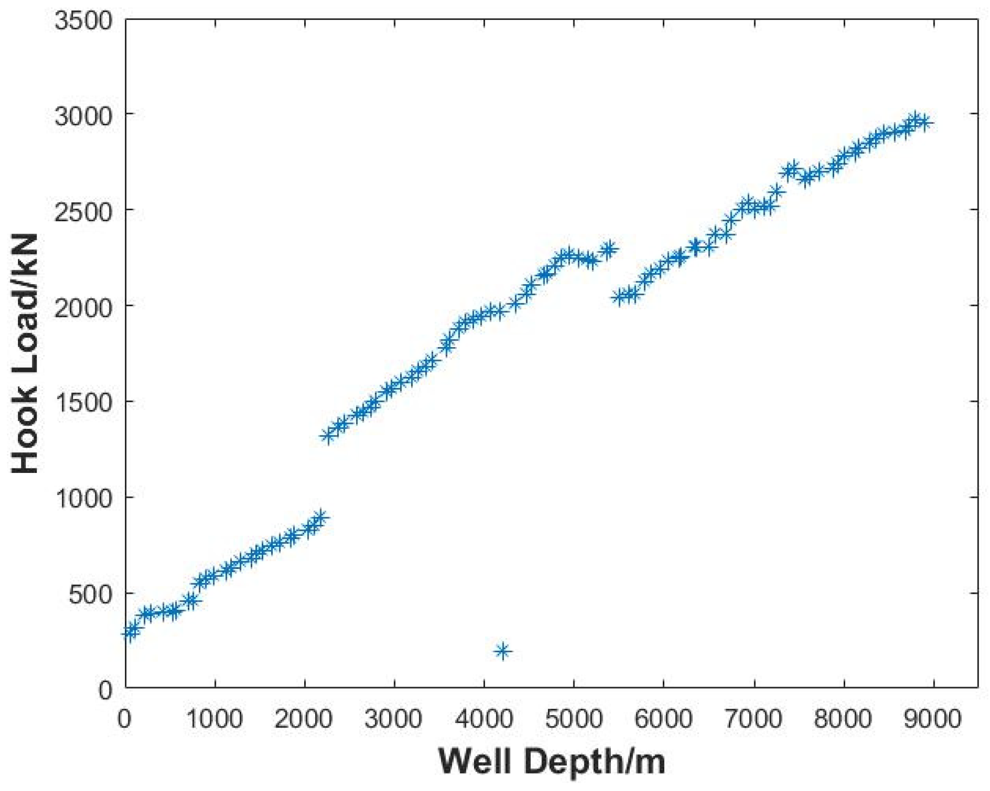
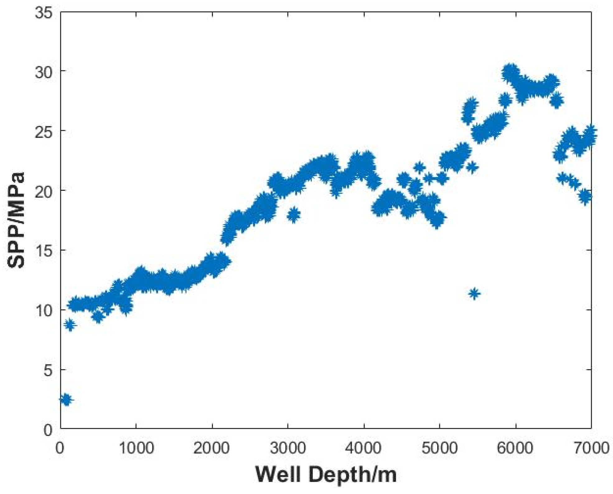
Fourthly, primary data cleansing is carried out based on the assumption of each data density threshold. The data density of each grid is compared with the assumed data density threshold, and the data in the grid below the data density threshold is cleared. The remaining data after the primary cleansing is obtained, and the two-dimensional scatter plot is drawn. The amount of cleared data is counted at the same time, and the total data volume before data cleansing is used as the benchmark to calculate the data cleansing percentage.

Finally, for each hypothetical data density threshold, the two-dimensional scatter plots before and after primary cleansing are compared. The largest possible data density threshold is selected as the optimal data density threshold on the premise of ensuring that the trend of the original data is retained and the data near the trend line is not obviously missing. The data cleansing percentage calculated based on the optimal data density threshold is recorded as the data cleansing percentage of the primary cleansing, and the remaining data after primary cleansing that correspond to the optimal data density threshold are saved for further processing.

2.2. Secondary Data Cleansing

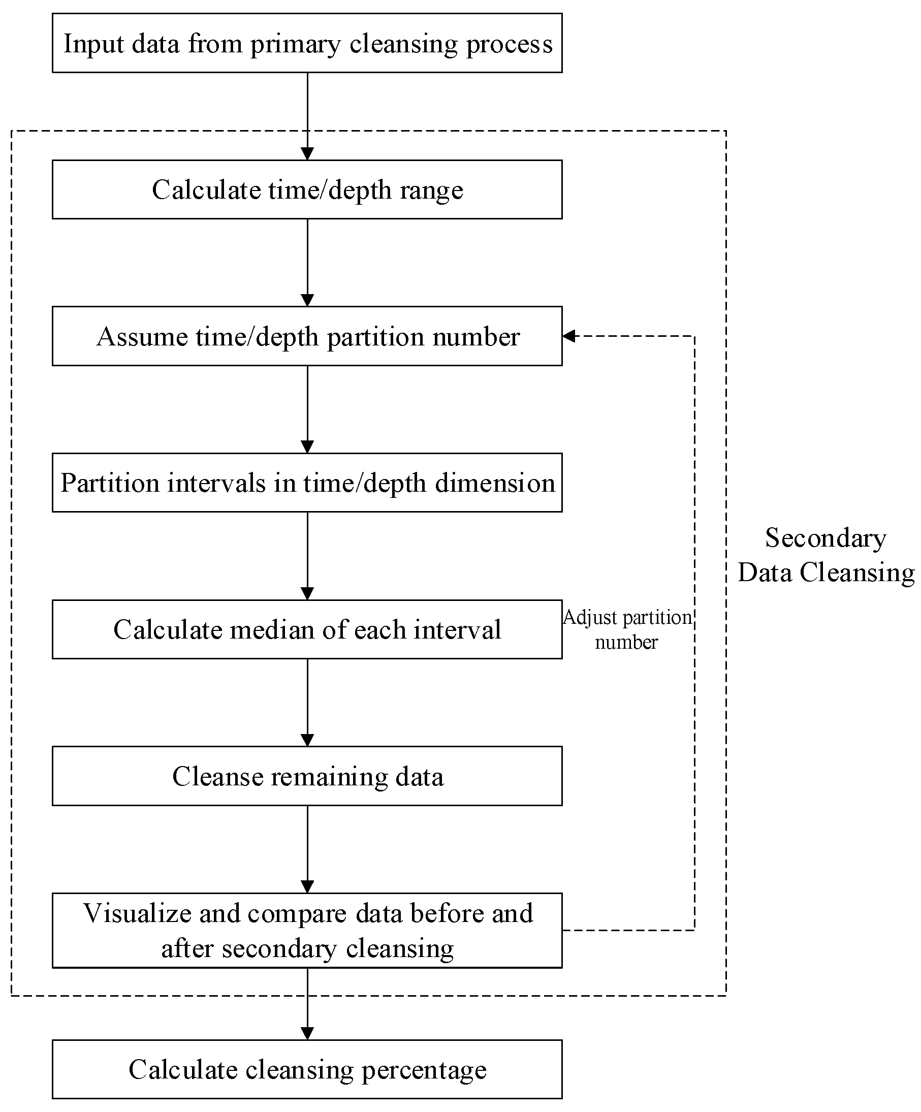
The secondary data cleansing is performed to accomplish further cleansing based on primary data cleansing on the premise of ensuring that there is no obvious loss of data near the trend line. The process of the secondary data cleansing is illustrated in Figure 3.

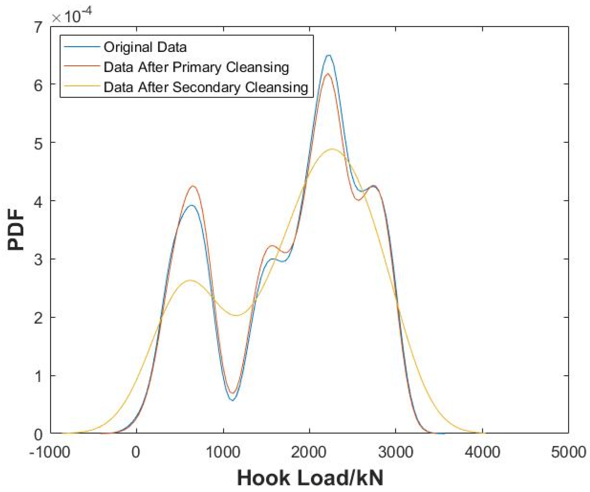
Firstly, after primary cleansing, the data is partitioned in one dimension using two methods: The first method is based on the previous two-dimensional partition grids, merging the data of the same time/depth intervals; that is, only the longitudinal partition boundary line is retained to form a series of time/depth intervals. The second method is performed to reset the partition interval or the partition number only for the time/depth (abscissa). Then, the median of the data subset at each time/depth interval is statistically calculated and retained, and the other data in the interval are cleared. The amount of cleared data is counted, and the total data volume before primary data cleansing is used as the benchmark to calculate the data cleansing percentage of the secondary cleansing. The data after the secondary cleansing are obtained, and the two-dimensional scatter plot is plotted. Finally, two-dimensional scatter plots of the data before cleansing, the data after primary cleansing, and the data after secondary cleansing are compared to ensure that the original trend of the data is retained globally.

2.3. Segmented Data Fitting

Well logging and drilling data present significantly different trending characteristics depending on downhole dynamic conditions and measuring equipment states. For well logging data, the function fitting method is usually selected based on the physical characteristics and the formation response relationship of the specific parameter. For parameters that have a linear or a simple non-linear relationship with depth, such as the acoustic transit time, the polynomial fitting method is appropriate. For parameters that are seriously affected by pore fluids or formation pressure, such as resistivity, the exponential fitting method is applicable. For parameters that involve more complicated non-linear relationships, machine learning methods need to be considered to obtain more accurate predictions. In addition, the key factor in choosing fitting functions is to consider formation or lithology changes, as well as subsurface fluid interfaces. The solution in the paper is to perform automated segmented function fitting based on similar criteria comparison among adjacent data so that data that follow different trends can be fitted separately. For drilling parameters, the function fitting method is selected based on drilling conditions. For normal drilling conditions, the lower-order polynomial fitting method is applicable to fit the slow trends of parameters such as weight on the bit (WOB) and torque. During tripping operations, the key point is to precisely identify different phases and abrupt changing points and then perform function fitting in segments. For circulation conditions, the constant fitting method is appropriate for most parameters that remain steady during the process, and the exponential fitting method is needed to fit gradually changing parameters such as temperature. During operations that involve making connections, polynomial fitting for different short-term windows is needed to perform transient data modeling. Overall, polynomial fitting and exponential fitting, combined with the data automated segmentation method, can satisfy the fitting requirements of most well logging and drilling data under different formation and drilling conditions.

After the automated cleansing process of the data, the outliers and duplicate values are greatly reduced. On this basis, the data after the secondary cleansing can be segmented and fitted. Then parameter values of any time/depth can be calculated, and the parameter data with a fixed time/depth interval can be output to realize multi-source data synchronization and can be used as input data for subsequent simulation calculation and intelligent analysis.

According to the characteristics of the data after the secondary data cleansing, the fitting function is assumed to be a polynomial or an exponential expression, and then the regression solution is carried out. Polynomial fitting is a method of approximating data points using a polynomial function, thereby determining the maximum order of the polynomial according to the complexity of the data. The expression of the polynomial function is as follows:

$$y={{\displaystyle \sum }}_{i=0}^n{a}_i{x}^i$$

(1)

where $a_i$ is the ith order term coefficient of the fitting polynomial; and $n$ is the maximum order of the fitting polynomial.

The expression of the exponential function is as follows:

$$y=k{b}^x\left(k>0,b>0,b\ne 1\right)$$

(2)

where $k$ is the coefficient of the fitting exponential function; and $b$ is the base of the fitting exponential function.

In order to fit the time/depth data after data cleansing in segments, it is necessary to traverse and compare all the data points. Through comparison, the adjacent data that meet the similar criteria are classified into the same subseries, and the fitting function type of the corresponding subseries is determined accordingly. Finally, mathematical statistical methods are used to solve the optimal value of the fitting coefficient vector to obtain the optimal fitting function of each subsequence. To solve the coefficients of fitting functions, different mathematical methods may be used, as long as the fitting results meet the specified accuracy requirements, such as least squares regression, ridge/lasso regression, and numerical approaches. Among different methods, the least squares method is applicable for small- to medium-scale datasets and is computationally efficient. In this paper, after data cleansing, the fitting function is assumed to be a polynomial or an exponential expression, and then the regression solution is carried out. The least squares regression can be selected because it is characterized by fast calculation and easy implementation for solving coefficients of lower-order polynomial functions. For exponential fitting, the expression can be converted to a linear equation, and then the least squares method can also be used to solve the fitting coefficient vector. To overcome the overfitting problem that may occur in the higher-order polynomial functions, the regularized least squares method can be used to solve the coefficients alternatively.

The mth derivative of the polynomial function in Equation (1) is shown as follows:

$${\displaystyle \frac{d{\left(a_0+a_{1}x+\cdots a_n{x}^n\right)}^{\left(m\right)}}{dx}}=m!a_m+\left(m+1\right)!a_{m+1}x+\cdots {\displaystyle \frac{n!}{\left(n-m\right)!}}{a}_n{x}^{n-m}$$

(3)

From the general form of the mth derivative of the polynomial function above, it can be deduced that the nth-order (highest) derivative of the polynomial function is as follows:

$${\displaystyle \frac{d{\left(a_0+a_{1}x+\cdots a_n{x}^n\right)}^{\left(n\right)}}{dx}}=n!a_n$$

(4)

According to Equation (4), the highest-order derivative of the polynomial function is a constant.

The first derivative of the exponential function in Equation (2) can be obtained as follows:

$${\displaystyle \frac{d\left(k{b}^x\right)}{dx}}=k{b}^x\ln b$$

(5)

Comparing Equations (2) and (5), the ratio of the first derivative of the exponential function to the function itself is a constant.

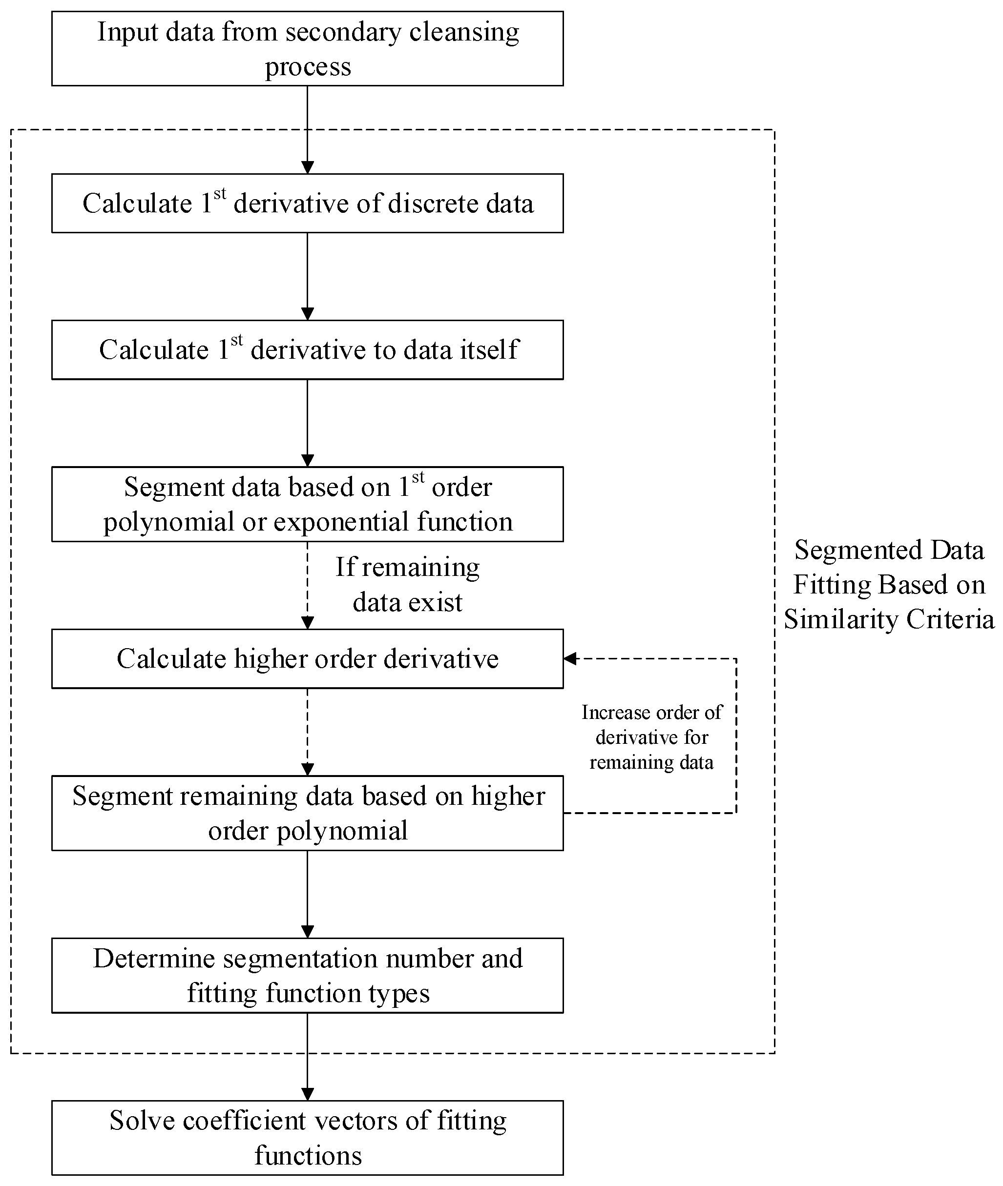
According to the characteristics of the polynomial function and the exponential function, the similarity criterion of each function can be determined. The number of segments and the function type of each segment is determined based on the similarity criteria of fitting functions. For the time/depth data after data cleansing, the first derivative is calculated using the differential equation of discrete data, and then the ratio of the first derivative to the data itself is calculated. Based on the hypothetical similarity, the first derivative and the ratio of the first derivative to the data itself are traversed and compared among all the cleansed data. The adjacent data that meet the same similarity criterion are classified into the same subsequence, and the fitting function type of the subsequence is determined accordingly. The adjacent data with a constant value of the first derivative are classified into a separate subset, and the fitting function of the subset is a first-order polynomial, which is a linear equation. The adjacent data with a constant ratio of the first derivative to the data itself are classified into a separate subset, and the fitting function of the subset is an exponential equation. For the remaining data that do not satisfy the two similar criteria mentioned above, the higher-order derivative is calculated, and the adjacent data are traversed and compared until the similarity criteria are met to divide all the data into subsets and determine the order of the fitting polynomial of each segment. The segmented data fitting process based on similarity criteria is illustrated in Figure 4.

The derivative of discrete data can be obtained using either the forward or backward differential as follows:

$$y_i^{\left(k+1\right)}={\displaystyle \frac{y_{i+1}^{\left(k\right)}-y_i^{\left(k\right)}}{x_{i+1}-x_i}}$$

(6)

$$y_i^{\left(k+1\right)}={\displaystyle \frac{y_i^{\left(k\right)}-y_{i-1}^{\left(k\right)}}{x_i-x_{i-1}}}$$

(7)

where $x_i$ is the time/depth value of the ith discrete data point; and $y_i^{\left(k\right)}$ is the kth order derivative of the ith discrete data point.

3. Case Study

The automated data cleansing method can be used to process the oilfield data recorded at a specific time/depth interval. The data need to be processed through primary cleansing and secondary cleansing procedures, and then missing values are supplemented through segmented fitting. Throughout the whole process, parameter data with any fixed frequency can be output. The data processing workflow is illustrated through example cases of hook load and stand pipe pressure data.

3.1. Hook Load Data Processing

The hook load parameter is a key parameter in drilling engineering that refers to the total vertical load on the hook during drilling, usually measured in real time by a hook load sensor at the top of the derrick. It directly reflects the weight of the drill string, downhole friction, drilling fluid buoyancy, and other dynamic loads and is an important basis for safety assessment and drilling operation optimization. The hook load data used in the case study are obtained from self-built databases composed of real-time drilling data, log data, Measurements While Drilling (MWD)/Logging While Drilling (LWD) data, etc. The reason for selecting the hook load parameter in the case study is that any abnormal increase in the parameter value can be interpreted as an early sign of drilling risks. Due to the dynamics of the hook load and its sensitivity to several factors, there is a high probability that there will be a lot of noise in the data. The large number of unreliable hook load data points and the requirements for the timeliness of data processing make it very important to perform data cleansing and function fitting in an automated workflow.

The scatter plot of the parameter hook load changing with depth for an example well is shown in Figure 5. According to the statistics, the total data volume before data cleansing is 8955. The depth range of the data is 61.00~9017.00 m, and the range of the hook load is 9.70~3140.50 kN.

In order to evaluate the data density of each area on the above-mentioned two-dimensional plot, the two-dimensional plot is divided into grids. The two-dimensional partition grids are equally spaced in terms of the two dimensions of well depth and hook load. The data density in each grid, which is the percentage of the data volume, is statistically calculated, and the three-dimensional statistical chart of data density distribution before data cleansing is shown in Figure 6.

The idea behind data cleansing is to keep the grids with higher data densities and eliminate the grids with lower data densities without destroying the overall trend. Therefore, the data densities of all the grids are statistically analyzed, and the data densities are sorted from large to small. The data density curve, with the grid sequence number as the abscissa and the grid data density as the ordinate, is drawn in Figure 7. In order to find the optimal data density threshold, the data density curve in Figure 7 is analyzed, and the coordinates of inflection points are labeled.

According to inflection points on the data density curve, it is assumed that the data density thresholds are 0.74, 0.45, 0.23, and 0.11. Using different data density thresholds, the primary cleansing is carried out. The data before cleansing and after primary cleansing based on different data density thresholds are compared in order to ensure that the original trend of the data is retained and the data near the trend line is not obviously missing. Based on this principle, the optimal data density threshold is determined to be 0.23, and the data cleansing percentage of primary cleansing is 17.43%. The data density distribution after primary cleansing is shown in Figure 8. The two-dimensional scatter plot of the hook load after primary cleansing is shown in Figure 9. By comparing the scatter plots between the hook load data before and after primary cleansing, it can be observed that the outliers are obviously cleared, and the overall trend of the data is not broken.

In order to further reduce the data amount, on the basis of primary cleansing, all the intervals of the hook load dimension are merged. According to the required amount of data cleansing, the well depth dimension can also be re-partitioned at larger or smaller intervals. The data at each well depth interval is statistically analyzed, and the median of the interval is retained. The data cleansing percentage of the secondary cleansing is 81.45%, which greatly reduces the total amount of data. The data after the secondary cleansing is shown in Figure 10. Comparing the hook load data before cleansing, after primary cleansing, and after secondary cleansing, it can be observed that after two-stage cleansing, outliers and duplicate values have been greatly eliminated, and the overall trend of the data is retained, with an overall cleansing percentage of 98.88%.

To validate the data cleansing processes, statistical distributions of original data, data after primary cleansing, and data after secondary cleansing are compared in Figure 11. To further guarantee the preservation of data distribution characteristics and determine if data cleansing percentages are appropriate, key statistical indicators are calculated and compared. The mean values of original data, data after primary cleansing, and data after secondary cleansing are 1802.60, 1776.60, and 1792.20, respectively. The changes in the mean values are less than 1.44%. The standard deviation values of original data, data after primary cleansing, and data after secondary cleansing are 825.02, 821.48, and 828.70, respectively. The changes in the standard deviation values are less than 0.45%.

After the automated cleansing process of the data, the curve trend of the hook load data with the depth of the well is obvious. The segmentation method and the fitting function type of each subsequence are determined according to the similar criteria, and the following fitting equations can be obtained through the segmented fitting:

$$y=-1.3355\times {10}^{-5}{x}^2+0.3053x+276.6025 \left(61\le x\le 2221\right)$$

(8)

$$y=-1.1464\times {10}^{-5}{x}^2+0.2917x+595.7348 \left(2221<x\le 4211\right)$$

(9)

$$y=-2.9231\times {10}^{-4}{x}^2+3.0933x-5910.2 \left(4211<x\le 5451\right)$$

(10)

$$y=-2.5217\times {10}^{-5}{x}^2+0.6444x-763.3276 \left(5451<x\le 9017\right)$$

(11)

To validate the function fitting process, some of the evaluation indicators are calculated. Among different segments, the MAE values are less than 18.82, the MAPE values are less than 3.66%, and the R² values are greater than 0.94.

The fitting curves are shown in Figure 12, and by applying the fitting formula described above, the hook load of any well depth can be calculated to output data of any specified frequency.

3.2. Stand Pipe Pressure Data Processing

In drilling engineering, stand pipe pressure (SPP) refers to the fluid pressure measured at the stand pipe as the drilling fluid flows downward through the inside of the drill string. It is one of the key real-time monitoring parameters during the drilling process that directly affects safety and efficiency. The scatter plot of the parameter SPP changing with depth for an example well is shown in Figure 13. The variation patterns of the SPP data are more complex than that of the hook load data. The reason is that SPP comprehensively reflects the dynamic interaction among hydraulic, mechanical, and geological factors in the drilling system and is highly sensitive to instantaneous disturbances.

Through grid partitioning and data density analysis based on the two-dimensional plot of the SPP data, the optimized data density threshold is 0.09, which is used to determine in which grids the data is to be cleansed. The three-dimensional statistical charts of data density distribution before and after primary data cleansing are shown in Figure 14 and Figure 15.

Through primary data cleansing, the cleansing percentage is 14.02%. The two-dimensional scatter plot of the SPP data after primary cleansing is shown in Figure 16. On the basis of primary cleansing, the secondary cleansing process is carried out through interval partitioning in the depth dimension and statistical calculation. The data after the secondary cleansing is shown in Figure 17. The data cleansing percentage of the secondary cleansing is 84.54%, with a two-stage cleansing percentage of 98.56%.

To validate the rationality of the data cleansing proportion and the preservation of the data distribution characteristics, the statistical distributions of the original data, data after primary cleansing, and data after secondary cleansing are compared in Figure 18. The mean values of the original data, data after primary cleansing, and data after secondary cleansing are 18.92, 18.82, and 18.75, respectively. The changes in mean values are less than 0.87%. The standard deviation values of the original data, data after primary cleansing, and data after secondary cleansing are 5.82, 5.83, and 6.02, respectively. The changes in standard deviation values are less than 3.44%.

After data cleansing, the segmented function fitting method is applied to determine the number of segments and fitting function types. The segmented fitting curves are shown in Figure 19. The SPP data variation patterns are complex, with the characteristics of multi-stage, non-linear, and abrupt changes, making the segmented function fitting process inevitable. The segmentation method is not only a technical necessity but also a guarantee of engineering safety. With accurate segmentation modeling, anomalies can be identified earlier, and drilling parameters can be optimized. To evaluate the function fitting performance, some of the evaluation indicators are calculated. Among different segments, the MAE values are less than 0.66, the MAPE values are less than 2.94%, and the R² values are greater than 0.80.

4. Conclusions and Suggestions

In this paper, an automated data cleansing and function fitting method for well logging and drilling data is established. Through this method, the data can be cleansed at primary and secondary levels. Combined with the segmented fitting of the cleansed data, the data output of any frequency can be obtained, which can be flexibly adapted to the synchronization requirements of subsequent simulation calculation and intelligent analysis.

The automated data cleansing method proposed in this paper deals with outliers, duplicate values, and missing values in an integrated manner. The case analysis shows that the method can significantly cleanse the data. The data cleansing percentage reaches 98.88% for the hook load data and 98.56% for the SPP data after two-stage cleansing, which still retains the original trend of the data and improves the efficiency and reliability of subsequent field calculations, analysis, and decision-making.

Future directions for extending the work in this paper include data characteristic analysis in the segmented function fitting process, and automation improvement of the data cleansing process. Firstly, for more accurate data modeling, data types and characteristics can be taken into consideration. For well logging data, machine learning methods can be utilized to predict the formation lithology and subsurface fluid type. For drilling data, machine learning methods can also be used to identify drilling conditions. Then, data of different types can be segmented and fitted accordingly. Secondly, the process of determining the data density threshold during primary cleansing can be automated by calculating the derivative of discrete data using differential methods. The derivatives can be traversed and compared among adjacent data to determine inflection points with sudden changes in the slope. For locally fluctuating data, to avoid threshold optimization difficulties and guarantee computational efficiency, visualization and manual adjustments can still be used as a complementary means. In addition, the segmented data fitting method proposed in this paper assumes that the fitting function type is polynomial or exponential, and the similarity criterion of each function is analyzed based on their characteristics. In order to improve the automation and reliability of the whole process, including data cleansing, data fitting, and data synchronization, types of fitting functions need to be expanded, and solution methods for determining fitting parameters need to be optimized.