Robust Optimization of Hydraulic Fracturing Design for Oil and Gas Scientists to Develop Shale Oil Resources

Abstract

Shale plays with pre-existing natural fractures can yield significant production when operating horizontal wells with multi-stage hydraulic fracturing (HWMHF). This work proposes a general, robust, and integrated framework for estimating optimal HWMHF design parameters in an unconventional naturally fractured oil reservoir. This work considers uncertainty in both the distribution of the natural fractures and uncertainty in three geo-mechanical parameters: the internal friction factor, the cohesion coefficient, and the tensile strength. Because a maximum of five design variables is considered, it is appropriate to apply derivative-free algorithms. This work considers versions of the genetic algorithm (GA), particle swarm optimization (PSO), and general pattern search (GPS) algorithms. The forward model consists of two linked software programs: a geo-mechanical simulator and an unconventional shale oil simulator. The two simulators run sequentially during the optimization process without human intervention. The in-house geo-mechanical simulator model provides sufficient computational efficiency so that it is feasible to solve the robust optimization problem. An embedded discrete fracture model (EDFM) is implemented to model large-scale fractures. Two cases strongly verified the feasibility of the framework for the optimization of HWMHF, and the average comprehensive NPV increases by 35% and 102.4%, respectively. By comparison, the pattern search algorithm is more suitable for HWMHF optimization. In this way, oil and gas scientists are contributing to the energy industry more accurately and resolutely.

1. Introduction

Horizontal well multi-stage hydraulic fracturing (HWMHF) has emerged as a cornerstone technology for the development of unconventional reservoirs, particularly shale oil and gas. In naturally fractured reservoirs, the interaction between hydraulic and natural fractures often results in the formation of a complex fracture network (CFN) rather than simple bi-wing planar fractures [1,2,3,4,5]. While HWMHF significantly enhances well productivity, the optimization process must account for uncertainties in natural fracture distribution and geo-mechanical parameters. The success of HWMHF optimization hinges on the precision and efficiency of fracture propagation models and reservoir simulation techniques.

Numerous analytical and numerical approaches have been developed to simulate fracture propagation. Mack et al. [6] introduced a pseudo-3D (P3D) model to estimate fracture height growth, but it is limited to bi-wing vertical planar fractures and cannot account for mechanical interactions between hydraulic and natural fractures. Xu et al. [7] proposed a wire-mesh model to simulate fracture activation patterns, considering mechanical interactions between fractures of the same orientation but neglecting orthogonal fracture interactions. Dahi-Taleghani and Olson [8] developed a model for nonplanar, pseudo-3D fracture propagation in naturally fractured reservoirs. However, it only considers simple fracture interactions due to the computational cost of the extended finite element method (XFEM). Wu and Olson [9] introduced a simplified model using the displacement discontinuity method (DDM) to simulate fracture propagation and fluid flow, incorporating stress-shadow effects and hydraulic-natural fracture interactions. However, their model cannot simulate bifurcation geometry when activating natural fractures, leading to discrepancies from real fracture geometries.

Reservoir simulation models have also evolved to simulate multiphase flow in naturally fractured reservoirs. The dual-porosity (DP) model, introduced by Warren and Root [10], was the first numerical dual-continuum approach. Pruess and Narasimhan [11] developed a dual porosity and dual permeability (DPDK) model to simulate heat and fluid flow in fracture systems. However, Moinfar et al. [12] found that the DP-DK model struggles in highly heterogeneous fracture systems. Wu and Pruess [13] introduced the multi-porosity model, MINC (multi-interactive continua), to replicate dynamic interactions between fractures and the matrix. However, continuum models, including MINC, are inadequate for modeling complex networks of natural and hydraulic fractures. Discrete-fracture models (DFMs) offer advantages, such as explicit representation of fracture geometry and flexibility in adapting to evolving fracture distributions. Li and Lee [14] and Moinfar et al. [15] described a distinctly different model (EDFM) for simulating flow in fractures. In the EDFM, a conventional orthogonal grid is employed for matrix representation, and additional fracture control volumes are introduced by calculating the intersection between fracture objects and the matrix cells. This work implements EDFM to simulate the multiphase flow in fractures created or activated by HWMHF. The EDFM can represent fractures having any orientation without regenerating the underlying Cartesian grids. Moreover, EDFM is very flexible for handling any fracture-fracture intersection and fracture-well connection. Therefore, EDFM can guarantee accuracy and efficiency when performing reservoir simulation in naturally fractured reservoirs.

The optimization problem in reservoir development typically involves maximizing a predefined objective function, such as cumulative oil/gas production or net present value (NPV) over the production cycle [16,17,18,19,20,21,22,23]. The general problem can include many different types of design variables, e.g., well paths, well controls (well pressure or rate at specified or adaptively selected time intervals (control steps), number of wells, type (injector or producer), and drilling order. To account for uncertainty in the reservoir characterization, one generally applies robust optimization, where instead of optimizing design variables for a fixed reservoir model, which is referred to as deterministic optimization, one maximizes the average cost function over a set of realizations that characterize the uncertainty in reservoir description. Maximizing the average NPV (often referred to loosely as the expected value) is commonly referred to as robust optimization. However, there exists a situation where it may be important to consider bi- or tri-objection optimization where the three objectives may maximize average life-cycle NPV and average short-term NPV [24,25,26]. Wilson and Durlofsky [27] proposed a framework to maximize NPV in Barnett shale development by optimizing well locations, lengths, and fracture stages. Ma et al. [28] compared gradient-based and gradient-free methods for optimizing well locations and fracture spacing in shale gas reservoirs, though natural fracture activation was not considered. Li et al.’s [29] design variables consist of both discrete and continuous variables, while no geo-mechanical effect and natural-hydraulic fracture interactions are considered in their work. To solve the associated mixed-integer optimization problem, a dynamic simplex interpolation-based alternate subspace (DSIAS) search method was applied. Wang and Chen [30] proposed a comprehensive optimization framework based on the generalized differential evolution (GDE) algorithm to maximize the life-cycle net present value (NPV) by optimizing key parameters, including well lengths, well spacing, fracture spacing, and fracture half-length. Their study focused on tight reservoirs with multi-well pad configurations, specifically addressing planar vertical fractures. Building on this work, Wang et al. [31] introduced a hybrid surrogate model combined with a transfer learning-based approach (SATS-WSF) to optimize well spacing and stage spacing in horizontal wells. This innovative methodology effectively leverages the synergy among multiple surrogate models, significantly improving the accuracy and reliability of the optimization process while reducing computational burden and decision-making challenges. Yao et al. [32] further advanced the field by optimizing fracturing parameters in shale gas reservoirs using a modified variable-length particle swarm optimization algorithm (MVPSO). Their findings revealed that optimized fractures exhibit complex propagation patterns, with a linear relationship between conductivity and fracture half-length. Li et al. [33] developed a hybrid ML-PSO model by integrating machine learning (ML) and particle swarm optimization (PSO) algorithms to overcome the limitations of current production forecasting techniques. By constructing a machine learning model and performing a sensitivity analysis, the most influential parameters affecting production and net present value (NPV) were identified. The optimization of fracturing parameters successfully increased the NPV, demonstrating the effectiveness of machine learning in optimizing the horizontal well design. In a related study, Lu et al. [34] integrated deep neural networks (DNN) with particle swarm optimization (PSO) to enhance production forecasting and fracturing parameter optimization in shale oil reservoirs. Their work established a comprehensive DNN model database, demonstrating the superior performance of DNN models in production forecasting. Additionally, the PSO-based optimization significantly improved oil production and NPV. Zhang and Sheng [35] employed an improved neural network algorithm (M-NNA) combined with the displacement discontinuity method (DDM) and embedded discrete fracture model (EDFM) to investigate fracture propagation and productivity in shale gas reservoirs with natural fractures. By optimizing reservoir parameters with NPV as the objective function, their study achieved higher economic returns. Despite these advancements, a critical limitation persists in the existing literature: none of the aforementioned studies incorporates geo-mechanical effects. Consequently, they neglect the important interactions between hydraulic fractures and pre-existing natural fractures during the HWMHF process. This oversight limits the applicability of these methods in naturally fractured reservoirs, where geo-mechanical interactions play a pivotal role in fracture propagation and reservoir performance [36,37,38,39].

In this work, the geo-mechanical simulator and unconventional reservoir simulator are integrated to produce the complete forward model used in the optimization algorithms. The HWMHF design is optimized by incorporating the geo-mechanical effects to generate the complex fracture network (CFN). The DDM is the numerical method used to simulate the evolving geomechanics, i.e., changing stress field, during the fracturing process. Unlike the DDM developed by Wu and Olson [40], the bifurcation of activated fractures is considered in the model. To account for the uncertainty in the distribution of natural fractures and the uncertainty in geo-mechanical parameters, robust optimization is applied. Three different derivative-free algorithms, namely the genetic algorithm (GA), particle swarm optimization (PSO), and general pattern search, are employed to optimize the life-cycle average NPV of production from wells with fractures in a naturally fractured shale oil reservoir. This work considered the most important design (optimization) variables: fracture spacing, stage spacing, treatment pressure, and treatment volume. The cost function that is minimized includes the average net present value of production over a specified period adjusted by drilling and fracturing treatment costs. When well spacing is included as a design variable, the cost of leasing acreage may also be included in the cost function. The general organization of the paper is as follows: In the first section, the DDM, which is implemented to simulate the fracturing process in the naturally fractured reservoir, is introduced. Then, the optimization problem considered in this work is defined, which requires a definition of the cost function, the design (optimization variables), and a discussion of how uncertainties are incorporated. The results section consists of two examples, which are designed to illustrate the robustness of the optimal design framework.

2. Methodology

2.1. Displacement Discontinuity Method (DDM)

In the field of fracture mechanics, particularly in the accurate modeling of fracture displacement patterns and propagation trajectories, hydraulic fracturing technology plays a critical role. This study integrates the advanced theoretical framework of the two-dimensional displacement discontinuity method (DDM) [41,42] with a three-dimensional correction factor proposed by Olson [43] to systematically quantify normal ($D_n$) and shear ($D_s$) displacements, while comprehensively accounting for the complex effects of mechanical interactions. The two-dimensional DDM is based on the plane strain assumption, which idealizes the vertical dimension of the fracture as infinitely extending out-of-plane. However, this assumption becomes a limitation in real-world, high-pressure water-driven multiple hydraulic fracturing (HWMHF) scenarios, where the actual fracture height is often significantly smaller than its horizontal extent. To address this limitation, a three-dimensional correction factor is introduced in this study, refining the two-dimensional model to more accurately capture the displacement discontinuity induced by finite-height fractures. The mathematical formulation of this correction factor is derived from the research findings of Olson [43]:

$$H^{ij}=1-{\displaystyle \frac{{\mathrm{d}}_{\mathrm{i}\mathrm{j}}^{2.3}}{[{\mathrm{d}}_{\mathrm{i}\mathrm{j}}^2+{\mathrm{h}}^2{]}^{\frac{2.3}{2}}}}.$$

(1)

where $d_{ij}$ represents the distance between the center of elements $i$ and $j$, and $h$ is the fracture height in the z-direction. For each Double-Dipole Matrix (DDM) element, ℎ remains constant.

Assuming a system with N elements, the normal stress ${\sigma }_n^i$ and shear stress ${\sigma }_s^i$ on the i th element can be used to solve the following equations to calculate the shear displacement discontinuity $D_s^j$ and the normal displacement discontinuity $D_n^j$ for any j th element.

$${\mathsf{\sigma }}_{\mathrm{n}}^{\mathrm{i}}=\sum _{\mathrm{j}=1}^{\mathrm{N}}{H}^{ij}{C}_{ns}^{ij}{D}_s^j+\sum _{\mathrm{j}=1}^{\mathrm{N}}{H}^{ij}{C}_{nn}^{ij}{D}_n^j$$

(2)

$${\mathsf{\sigma }}_{\mathrm{s}}^{\mathrm{i}}=\sum _{\mathrm{j}=1}^{\mathrm{N}}{H}^{ij}{C}_{ss}^{ij}{D}_s^j+\sum _{\mathrm{j}=1}^{\mathrm{N}}{H}^{ij}{C}_{sn}^{ij}{D}_n^j,$$

(3)

The matrix $C_{ns}^{ij}$ quantifies the elastic influence in a plane-strain scenario, illustrating how a shear displacement discontinuity at element j induces normal stress at element i. Similarly, $C_{nn}^{ij}$ represents the normal stress at element i resulting from an opening displacement discontinuity at element j. This concept extends analogously to $C_{nn}^{ij}$ and $C_{ns}^{ij}$, which describes the influence of shear and normal displacement discontinuities on shear and normal stresses, respectively.

2.2. Fracture Propagation and Hydraulic Natural Fracture Interaction

Accurately determining the extension length and direction of fractures is crucial in the dynamic process of fracture propagation. In the context of high-pressure water-driven multiple hydraulic fracturing (HWMHF), the predominant failure mechanisms include Mode I (tensile opening) and Mode II (shear sliding) loading modes, which often coexist in mixed forms in real-world scenarios. To address this complexity, the present study adopts the mixed-mode fracture propagation criteria proposed by Sih (1963) [37] to scientifically and rigorously predict the fracture propagation length and direction.

According to Olson, the direction of fracture propagation is determined as

$$\tan {\displaystyle \frac{\mathsf{\theta }}{2}}={\displaystyle \frac{1}{4}}{\displaystyle \frac{K_{\mathrm{I}}}{K_{\mathrm{I}\mathrm{I}}}}\pm \sqrt{({\displaystyle \frac{K_{\mathrm{I}}}{K_{\mathrm{I}\mathrm{I}}}}{)}^2+8}.$$

(4)

The values of the stress intensity factors ($K_{\mathrm{I}}$ and $K_{\mathrm{I}\mathrm{I}}$) must be known to compute the propagation direction from Equation (4). The stress intensity factors can be computed as

$$K_{\mathrm{I}}={\displaystyle \frac{0.806\mathrm{E}\sqrt{\mathsf{\pi }}}{4\left(1-{\mathrm{v}}^2\right)\sqrt{2\mathrm{a}}}}{\mathrm{D}}_{\mathrm{n}},$$

(5)

$$\begin{array}{r}\\ K_{\mathrm{I}\mathrm{I}}={\displaystyle \frac{0.806\mathrm{E}\sqrt{\mathsf{\pi }}}{4\left(1-{\mathrm{v}}^2\right)\sqrt{2\mathrm{a}}}}{\mathrm{D}}_{\mathrm{s}}.\end{array}$$

(6)

where $E$ is Young’s modulus in the unit of MPa; $v$ is Poisson’s ratio; $D_n$ and $D_s$ are the normal and shear displacement discontinuity at the tip element, both in the unit of m; and $a$ is the half length of the tip element in units of m. $K_{I,c}$ and $K_{II,c}$ represent the values the critical stress intensity factors, corresponding to $K_I$ and $K_{II}$, respectively. Then a fracture will propagate whenever its $K_I>K_{I,c}$ or $K_{II}>K_{II,c}$.

Two scenarios may occur at the instant a propagating fracture meets a pre-existing natural fracture. The first possibility is that the propagating fracture crosses the natural fracture and continues its direction of propagation without activating the natural fracture. The second possible scenario is that the stress field induced by the hydraulic fracture triggers slippage along the natural fracture interface, resulting in the hydraulic fracture being captured and redirected by the natural fracture. The critical factor determining these outcomes is the hydraulic reactivity of the natural fracture, defined by whether interfacial slippage occurs. For frictional surfaces, slippage initiates when the shear stress exceeds the shear strength of the fracture interface, governed by the Coulomb failure criterion:

$$\left|{\tau }_{\beta }\right|>S_0+\mu {\sigma }_{n,\beta },$$

(7)

where ${\tau }_{\beta }$ and ${\sigma }_{n,\beta }$ represent the shear and normal stresses on the existing fracture interface; $\beta$ denotes the angle between the propagating fracture and the pre-existing fracture; $\mu$ is the internal frictional factor (dimensionless) of the fracture surface; and $S_0$ (MPa) is the cohesion coefficient of the fracture surface. Note that if the fracture is cemented, then the value of $S_0$ will be greater than $0$. The values of ${\tau }_{\beta }$and ${\sigma }_{n,\beta }$ can be determined by projecting the stresses onto the fracture surface using the following two equations:

$$\begin{array}{rr}& \\ & \end{array}{\mathsf{\tau }}_{\mathsf{\beta }}=-{\displaystyle \frac{{\mathsf{\sigma }}_{\mathrm{x}\mathrm{x}}-{\mathsf{\sigma }}_{\mathrm{y}\mathrm{y}}}{2}}\sin 2\mathsf{\beta }+\sin 2\mathsf{\beta }{\mathsf{\sigma }}_{\mathrm{x}\mathrm{y}},$$

(8)

$${\mathsf{\sigma }}_{\mathrm{n},\mathsf{\beta }}={\displaystyle \frac{{\mathsf{\sigma }}_{\mathrm{x}\mathrm{x}}+{\mathsf{\sigma }}_{\mathrm{y}\mathrm{y}}}{2}}-{\displaystyle \frac{{\mathsf{\sigma }}_{\mathrm{x}\mathrm{x}}-{\mathsf{\sigma }}_{\mathrm{y}\mathrm{y}}}{2}}\cos 2\mathsf{\beta }-\sin 2\mathsf{\beta }{\mathsf{\sigma }}_{\mathrm{x}\mathrm{y}}.$$

(9)

Recall that ${\sigma }_{xx}$, ${\sigma }_{yy}$, and ${\sigma }_{xy}$ are states of stress in the global coordinate system at the fracture tip.

2.3. Optimization of Fracture Design

The optimization problem under investigation focuses on determining the optimal design parameters for multi-stage hydraulic fracturing of horizontal wells. In this study, the optimization problem is formulated by maximizing the expected NPV, which is a standard approach in reservoir development. However, alternative formulations such as bi-objective optimization balancing life-cycle NPV and short-term cash flow, or minimizing risk measures like NPV variance, are also viable. Key design variables include stage spacing, fracture spacing, treatment pressure, and treatment volume. For scenarios involving simultaneous optimization of two wells, well spacing is added as a fifth parameter. The objective is to maximize the net present value (NPV) of the project by minimizing the negative NPV, which accounts for drilling costs, fracturing costs, and production revenue over the reservoir’s lifetime. The vector m denotes the uncertain reservoir/fracture model parameters, which include the probability distributions of the natural fracture parameters (fracture spatial distribution, fracture length, and fracture orientation). Given the fracture intensity (number of fractures per unit area), it assumes that the fracture’s spatial distribution follows a uniform distribution, and for each fracture distribution, the corresponding values of natural fracture length and orientation are drawn from Gaussian distributions. The vector m also includes uncertain geo-mechanical parameters, namely, the natural fracture cohesion coefficient, frictional factor, and tensile strength. The values of these parameters are generated for each fracture in the naturally fractured reservoir. It assumes that the random geo-mechanical variables (fracture cohesion coefficient, frictional factor, and tensile strength) have prescribed Gaussian distributions. Note that a realization of m is required to determine the complex network of fractures (hydraulic plus activated natural fractures) created by a fracking operation.

The vector u represents the combination of hydraulic fracturing design parameters. In the case of single-well fracturing optimization, u consists of four key variables: stage spacing, fracture spacing, treatment pressure, and treatment volume. For scenarios involving simultaneous optimization of two wells, well spacing is incorporated as a fifth optimization parameter. The primary objective is to determine the optimal values of these parameters to minimize the negative net present value (NPV) associated with drilling, fracturing, and production activities over the well’s lifetime. It is important to note that minimizing the negative NPV is equivalent to maximizing the NPV. The objective function is formally defined as follows:

$$J\left(\mathit{u},\mathit{m}\right)=-NP{V}_{\mathrm{project}}=-\left(NP{V}_{\mathrm{prd}}-C_{\mathrm{drill}}-C_{\mathrm{frac}}\right),$$

(10)

In this context, the net present value (NPV) associated with the well development project, denoted as $NP{V}_{\mathrm{project}}$, is composed of several key financial components. These include the NPV over the entire life cycle of the project, referred to as $NP{V}_{\mathrm{prd}}$, alongside the costs associated with drilling, represented by $C_{\mathrm{drill}}$, and the expenses incurred during the fracturing process, denoted as $C_{\mathrm{frac}}$.

The economic NPV of production from a multi-stage hydraulically fractured well is defined as:

$$NP{V}_{\mathrm{prd}}=\sum _{n=1}^{N_{\mathrm{t}}}{\displaystyle \frac{\Delta t_n}{{\left(1+b\right)}^{\frac{t_n}{365}}}}\left[\left(r_{\mathrm{o}}\cdot {\overline{q}}_{\mathrm{o}}^n\left(u,m\right)+r_{\mathrm{g}}\cdot {\overline{q}}_{\mathrm{g}}^n\left(u,m\right)-r_{\mathrm{w}}\cdot {\overline{q}}_{\mathrm{w}}^n\left(u,m\right)\right)\right],$$

(11)

where $t_n$ represents the time at the end of the n_th simulation time step, $\Delta t_n$ represents the duration of the n_th time step, and $N_{\mathrm{t}}$ represents the total number of time steps. For each n_th time step, the average production rates of oil, water, and gas are indicated by ${\bar{q}}_{\mathrm{o}}^n$ (measured in stock tank barrels per day, STB/D), ${\bar{q}}_{\mathrm{w}}^n$ (measured in stock tank barrels per day, STB/D), and ${\bar{q}}_{\mathrm{g}}^n$ (measured in thousand cubic feet per day, Mcf/D), respectively. The oil, gas, and water production rates used in Equation (11) are obtained from the unconventional reservoir simulator, which is based on the Embedded Discrete Fracture Model (EDFM). This simulator takes as input the fracture geometry and apertures generated by the DDM-based geo-mechanical simulator and solves multiphase flow equations to simulate production dynamics throughout the reservoir’s lifetime. The revenue associated with oil production is represented by the oil price $r_{\mathrm{o}}$ (USD/STB), while the revenue from gas production is represented by the gas price $r_{\mathrm{g}}$(USD/Mcf). Additionally, the cost associated with the disposal of produced water is denoted by $r_{\mathrm{w}}$ (USD/STB). The discount rate is denoted by b.

The estimation of drilling costs for horizontal wells poses significant complexities and challenges, stemming from dual difficulties in data collection and utilization, as well as inherent constraints within the modeling process. The research conducted by Kaiser [44] has contributed a series of statistical models aimed at achieving precise predictions of drilling costs. Following Kaiser’s [44] work, the comprehensive drilling cost is defined here.

$${\mathrm{C}}_{\mathrm{d}\mathrm{r}\mathrm{i}\mathrm{l}\mathrm{l}}=({\mathsf{\beta }}_0+{\mathsf{\beta }}_1\mathrm{L}+{\mathsf{\beta }}_2{\mathrm{L}}^2{)}^2$$

(12)

where ${\beta }_0$, ${\beta }_{1 }$, and ${\beta }_2$ are cost coefficients acquired from regression, and L is the lateral length of the horizontal well. The user can of course implement any model for drilling cost. It is important to note that the lateral length of the well is a dependent variable that is implicitly dependent on the number of fracture stages ($N_s$), number of hydraulic fractures ($N_f$) within one stage, fracture spacing ($L_f$), and stage spacing ($L_s$). Once those parameters are specified, the well length can be computed as

$$\mathrm{L}={\mathrm{N}}_{\mathrm{s}}\times \left({\mathrm{L}}_{\mathrm{f}}\times \left({\mathrm{N}}_{\mathrm{f}}-1\right)+2\times {\mathrm{L}}_{\mathrm{s}}\right).$$

(13)

In this work, each well has five stages with four fractures per cluster so $N_s=5$ and $N_f=4$. The fracturing cost is defined as

$$C_{\mathrm{frac}}=c_{\mathrm{fluid}}{V}_{\mathrm{fluid}}+c_{\mathrm{prop}}{V}_{\mathrm{prop}}+c_{\mathrm{pump}}{P}_{\mathrm{treat}},$$

(14)

where $c_{\mathrm{fluid}}$, $c_{\mathrm{prop}},$ and $c_{\mathrm{pump}}$ denote the unit cost of fracturing fluid, proppant, and pumping, respectively. $V_{\mathrm{fluid}}$ and $V_{\mathrm{prop}}$ respectively, denote the volume of fracturing fluid and the volume of proppant used during the treatment. $c_{\mathrm{pump}}$ denotes the cost of the pump. Since more pumping equipment is required to provide higher treatment pressure, it assumes that the total pump cost is proportional to the treatment pressure. This work multiplies the pump cost with the treatment pressure to obtain the total cost of the pumping equipment. $V_{\mathrm{fluid}}$, the volume of fracturing fluid used during the fracturing operation, is equal to the volume of fractures ($V_{\mathrm{frac}}$) plus the volume of leak-off ($V_{\mathrm{leak}}$). $V_{\mathrm{frac}}$ is calculated with the DDM geo-mechanical simulator. $V_{\mathrm{leak}}$ is computed by

$${\mathrm{V}}_{\mathrm{leak}}=\sum _{\mathrm{i}=1}^{{\mathrm{N}}_{\mathrm{ele}}}({\mathrm{q}}_{\mathrm{l},\mathrm{i}}({\mathrm{t}}_{\mathrm{i}})\times {\mathrm{t}}_{\mathrm{i}})$$

(15)

where $N_{\mathrm{ele}}$ denotes the number of DDM elements. The variable $t_i$ indicates the total duration of leak-off for the $i$th element, defined as the time interval from when element $i$ first began to experience leak-off up to the current time; $q_{l,i}\left(t\right)$ (${\mathrm{m}}^3/\mathrm{s}$) is the leak-off volume rate of the element $i$ at time $t_i$ calculated by the Carter model [36], which is given by

$${\mathrm{q}}_{\mathrm{l},\mathrm{i}}\left(\mathrm{t}\right)={\displaystyle \frac{2\mathrm{h}{\mathrm{L}}_{\mathrm{i}}{\mathrm{C}}_{\mathrm{L}}}{\sqrt{{\mathrm{t}}_{\mathrm{i}}}}}$$

(16)

where $C_L$ ($\mathrm{m}/\sqrt{\mathrm{s}}$) represents the fluid leak-off coefficient; $h$ represents the fracture height and $L_i$ (m) represents the length of $i$th element, respectively. Carter’s model assumes constant pressure within the fracture. Under the assumed framework, the treatment pressure during fracture propagation is considered constant, and no attenuation of pressure within the hydraulic fracture as it extends is taken into account.

In the development of unconventional reservoirs, the optimization of well spacing, a critical parameter parallel to the fracture design of single multi-stage fractured wells, is of paramount importance. Excessively narrow spacing can lead to overlapping production zones, triggering dynamic fluid interactions between wells, thereby constraining individual and overall, well productivity. Conversely, overly large spacing implies underutilization of reservoir resources, impacting economic development efficiency, particularly the failure to maximize returns from land leases. Thus, the rational determination of well spacing is crucial for balancing efficient reservoir exploitation with economic benefits. To include the well spacing as a parameter in the optimization problem, this work lets $C_{\mathrm{lease}}$ denote the cost of the land lease ($C_{\mathrm{lease}}$ as 6$\times {10}^6$ USD/km² in the example) and add this cost as an extra term in the objective function, i.e., redefine the objective function for the well spacing optimization problem by

$$J\left(u,m\right)=-NP{V}_{\mathrm{project}}=-\left(NP{V}_{\mathrm{prd}}-C_{\mathrm{drill}}-C_{\mathrm{frac}}-C_{\mathrm{lease}}\right),$$

(17)

where $C_{\mathrm{lease}}$ can be calculated as

$$C_{\mathrm{lease}}={\mathrm{L}}_{\mathrm{lateral}}\times {\mathrm{L}}_{\mathrm{spacing}}\times c_{\mathrm{lease}}.$$

(18)

In Equation (18), ${\mathrm{L}}_{\mathrm{lateral}}$ (m) represents the lateral length controlled by a fractured well, which is correlated to the well length by the equation ${\mathrm{L}}_{\mathrm{lateral}}=\mathrm{L}+2\times {\mathrm{L}}_{\mathrm{pad}}$; see Figure 1. ${\mathrm{L}}_{\mathrm{spacing}}$ (m) is the well spacing between two horizontal wells and $c_{\mathrm{lease}}$ is the cost of lease per area in the unit of $\mathrm{U}\mathrm{S}\mathrm{D}/{\mathrm{m}}^2$.

To address geological uncertainty, this study employs robust optimization by minimizing the average negative net present value (NPV) across an ensemble of realizations of the reservoir model m. Specifically, the expected value of the comprehensive NPV is approximated by the mean NPV computed over all realizations. Accordingly, the objective function for robust optimization is formulated as follows:

$$\overline{\mathrm{J}}\left(\mathrm{u}\right)\equiv {\displaystyle \frac{1}{{\mathrm{N}}_{\mathrm{e}}}}\sum _{\mathrm{k}=1}^{{\mathrm{N}}_{\mathrm{e}}}\mathrm{J}\left(\mathbf{u},{\mathbf{m}}_{\mathbf{k}}\right)\approx \mathrm{E}\left[\mathrm{J}\left(\mathrm{u},\mathrm{m}\right)\right],$$

(19)

Here, the expected value is denoted by $E$. The variable $N_{\mathrm{e}}$ represents the number of reservoir models used to account for geological uncertainty, with different models defined by ${\mathit{m}}_{\mathit{j}}$,where $j=1.2,\cdots N_{\mathrm{e}}$. It is important to note that evaluating of $\overline{J}\left(\mathit{u}\right)$ requires $N_{\mathrm{e}}$ forward simulation runs, resulting in high computational costs for each iteration of the objective function in robust optimization when N_e is substantial. Evaluating $\overline{J}\left(\mathit{u}\right)$requires $N_{\mathrm{e}}$ forward simulations, resulting in significant computational costs in robust optimization when $N_{\mathrm{e}}$ is large. Despite the existence of methods to improve computational efficiency by selecting a subset of $N_{\mathrm{e}}$ models, these approaches are not considered here.

Upon the establishment of the objective function, the optimization problem is clearly defined.

$$\underset{\mathit{u}\in R^{N_u}}{\mathit{min}}\overline{J}\left(\mathit{u}\right)$$

(20)

$$\mathrm{s}\mathrm{u}\mathrm{b}\mathrm{j}\mathrm{e}\mathrm{c}\mathrm{t} \mathrm{t}\mathrm{o} {\mathrm{u}}_{\mathrm{i}}^{\mathrm{l}\mathrm{o}\mathrm{w}}\le {\mathrm{u}}_{\mathrm{i}}\le {\mathrm{u}}_{\mathrm{i}}^{\mathrm{u}\mathrm{p}},\mathrm{i}=\mathrm{1,2},\dots ,{\mathrm{N}}_{\mathrm{u}},$$

(21)

where u denotes the design vector (vector of optimization variables), which includes the fracture spacing, stage spacing, treatment volume, and treatment pressure, if more than one well is present, well spacing will also be considered. The number of stages and the number of fractures per stage are predefined. Throughout, $u_i^{\mathrm{up}}$ and $u_i^{\mathrm{low}}$ denote the upper bound and lower bound of the $i\mathrm{t}\mathrm{h}$ controllable. Given that the optimization problem involves only four or five parameters (depending on whether well spacing is considered) involved in the optimization problem, the derivative-free optimization algorithms are viable. Three different such algorithms, GA, PSO, and PS, are tested on this problem. Additionally, gradient-based algorithms with finite difference gradients and StoSAG were implemented and tested on this workflow. However, both derivative-based algorithms resulted in lower values of the optimal average NPV than those obtained with the derivative-free algorithms. The observed inferior performance is likely attributed to the ruggedness of the objective function’s surface, compounded by the discretization errors introduced by EDFM. Consequently, the results from the gradient-based algorithms are not further analyzed in this study.

Figure 2 illustrates the operational workflow of the HWMHF design framework in detail. To ensure robust optimization, $N_e$ samples of m are drawn from predefined probability density functions. This results in a set of distributions representing the natural fracture system, along with corresponding samples of three geo-mechanical parameters. Each realization of m, along with the corresponding design parameter realizations, is fed into the in-house DDM-based geo-mechanical simulator. The geo-mechanical simulator used in this work is based on the two-dimensional Displacement Discontinuity Method (DDM), with a three-dimensional correction factor to account for finite-height fractures. It captures mechanical interactions and fracture reactivation under varying stress conditions.

The reservoir simulator incorporates an Embedded Discrete Fracture Model (EDFM), which allows for the efficient modeling of multiphase flow in complex fracture networks without regenerating the grid. The two simulators are coupled sequentially in the optimization workflow, enabling the dynamic transfer of fracture geometries and apertures.

The geo-mechanical simulator produces the simulated fracture pattern and corresponding fracture apertures, which are subsequently fed into the unconventional reservoir simulator. The fracture treatment cost is computed based on the geo-mechanical simulator’s input and output. The production revenue is derived from the reservoir simulator output. Finally, the average NPV, as defined in Equation (19), is computed. The optimization algorithm iterates to update design vectors, repeating the loop until termination. While the present study adopts a synthetic case approach, future work will focus on validating the model predictions with field production and microseismic data to enhance the reliability of the economic analysis [45,46].

Based on the integrated simulation-optimization workflow, the following hypotheses are proposed:

(1)

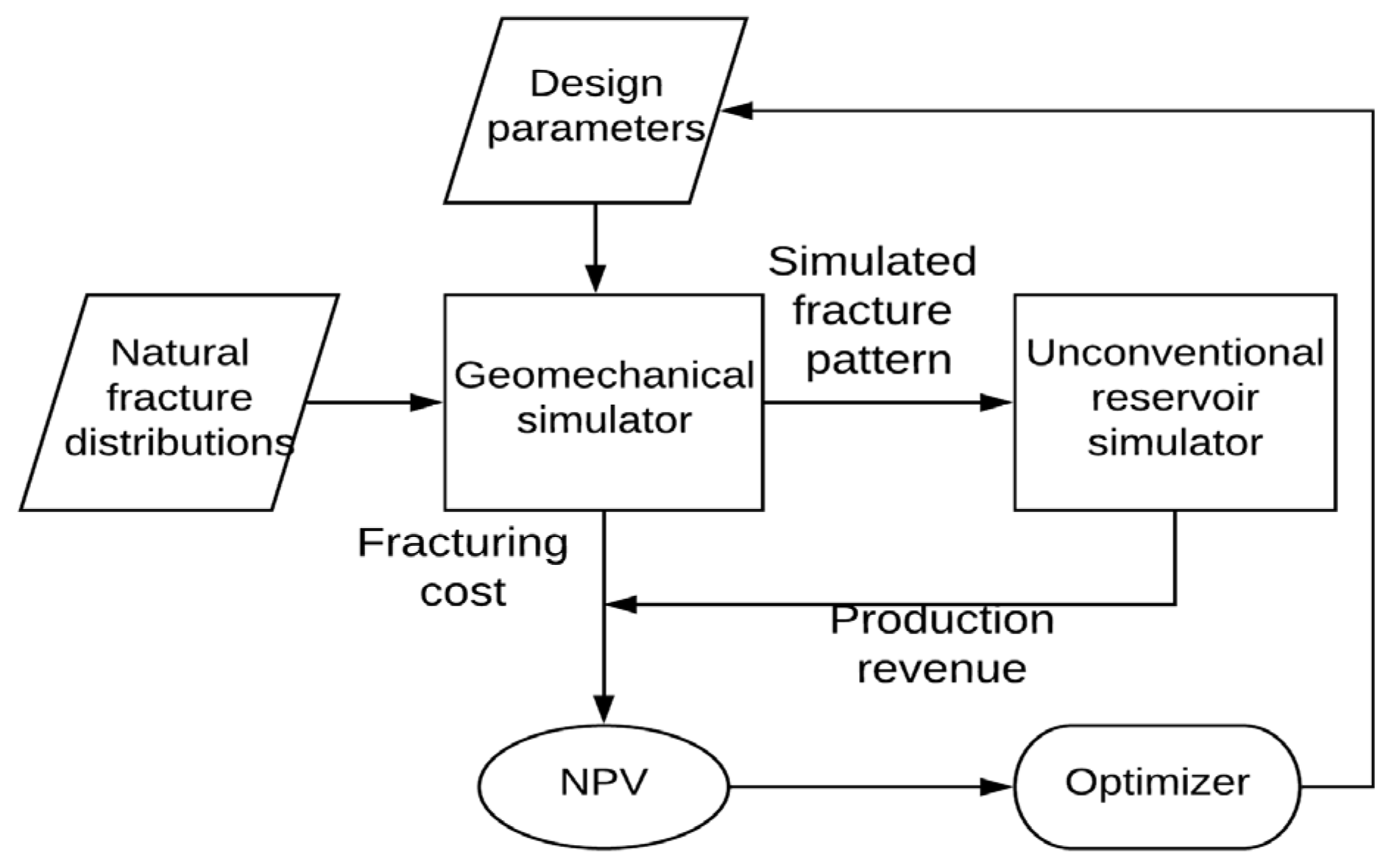
The sequential coupling of DDM-based geo-mechanical simulation and EDFM-based reservoir simulation can effectively represent fracture propagation and flow in naturally fractured reservoirs;

(2)

Incorporating geological and geo-mechanical uncertainties improves the robustness of NPV-based design decisions;

(3)

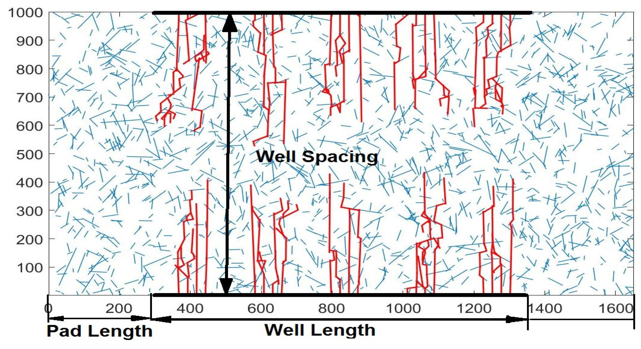
The inclusion of well spacing as a design variable significantly influences drainage efficiency and economic performance in multi-well development scenarios.

3. Computational Results

This section presents two case studies demonstrating the HWMHF design process for optimizing multi-stage hydraulic fracturing parameters in naturally fractured reservoirs. The first case meticulously focuses on the refinement of fracturing design parameters for a single well. The second case extends beyond single-well optimization, simultaneously optimizing well spacing and fracturing design parameters while integrating land leasing costs into the objective function. Additionally, the study explores the uncertainties in geo-mechanical parameters, such as the internal friction angle and cohesion coefficient, assuming that horizontal wells are drilled precisely along the maximum stress direction in the x-y plane.

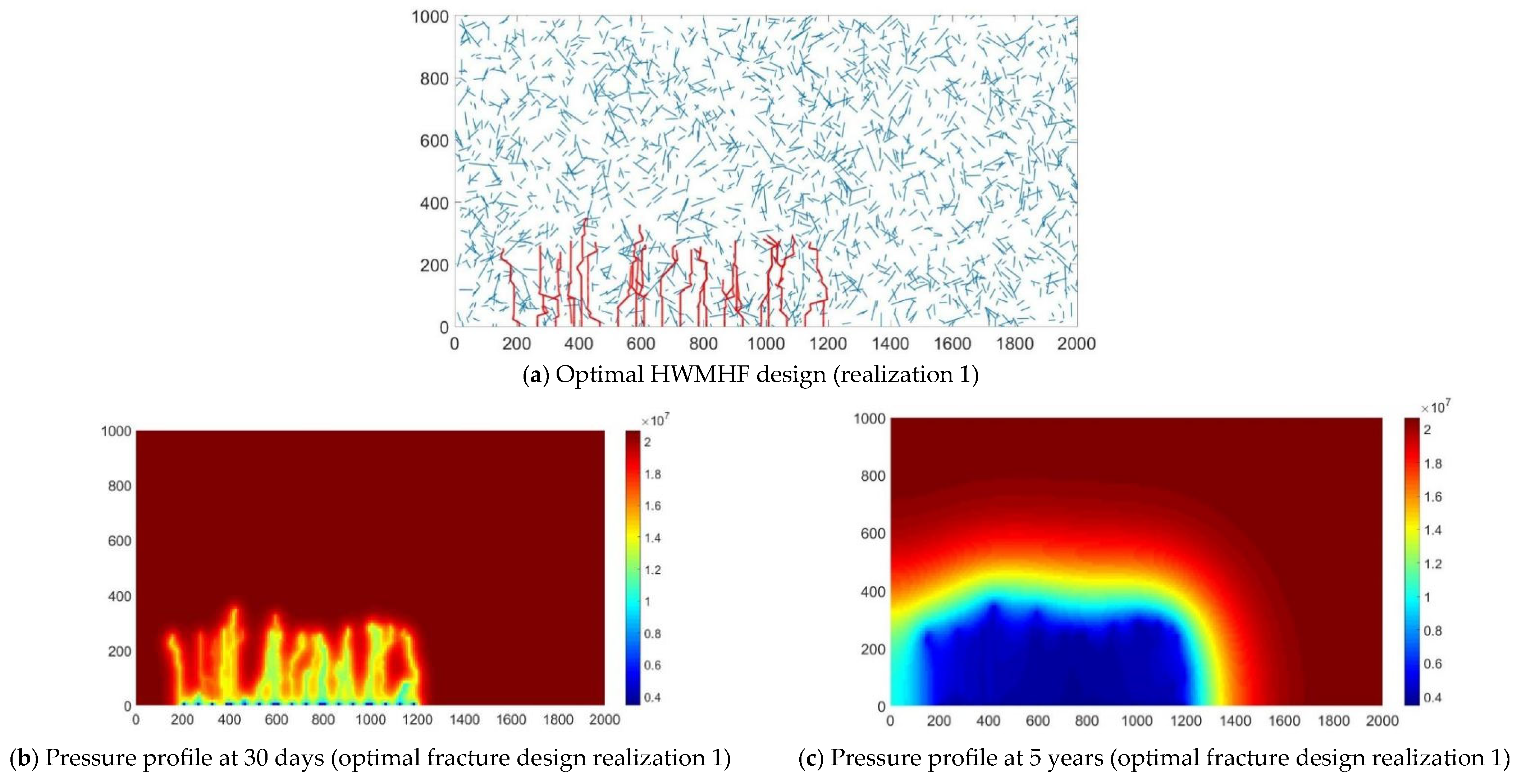
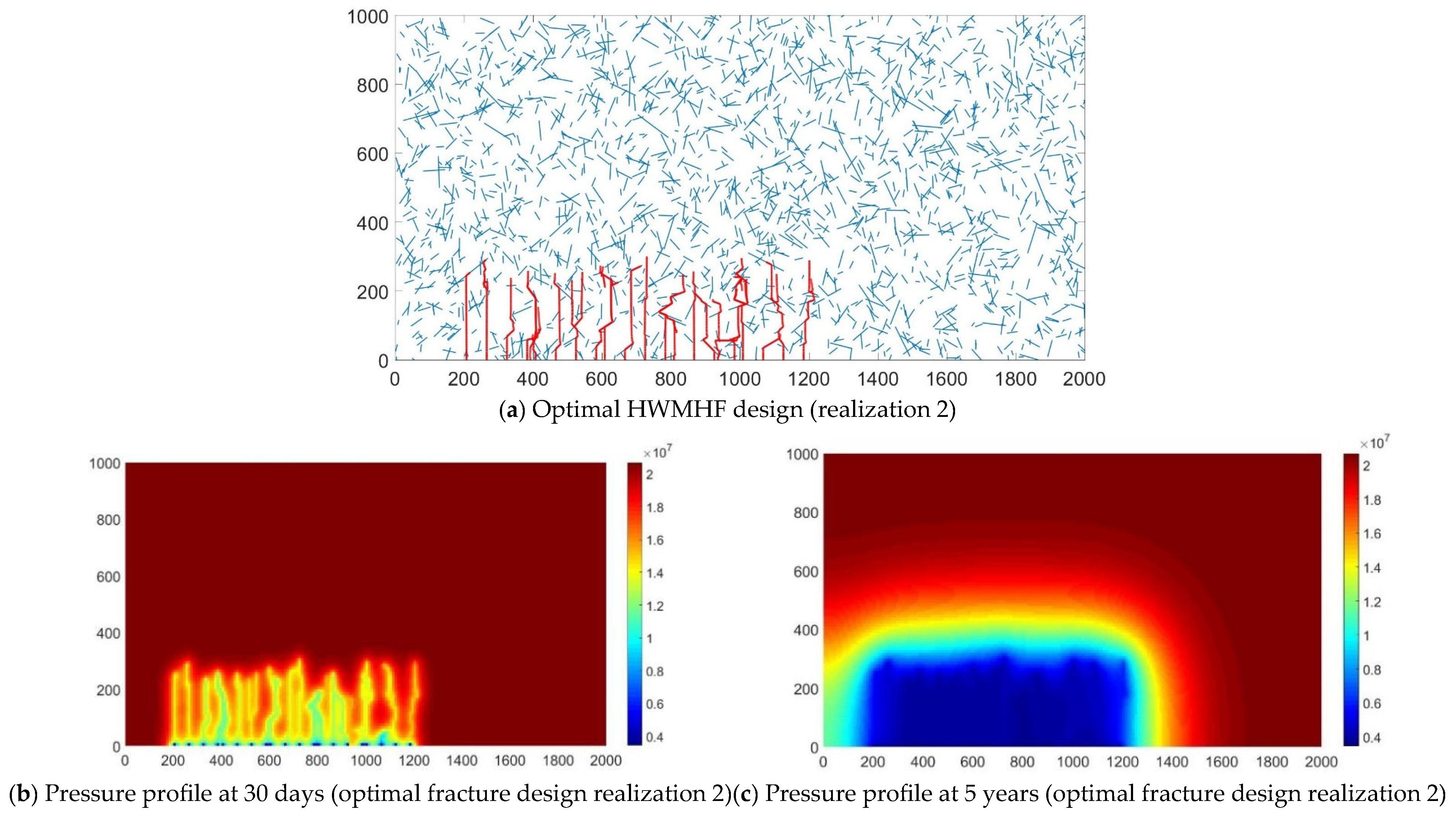
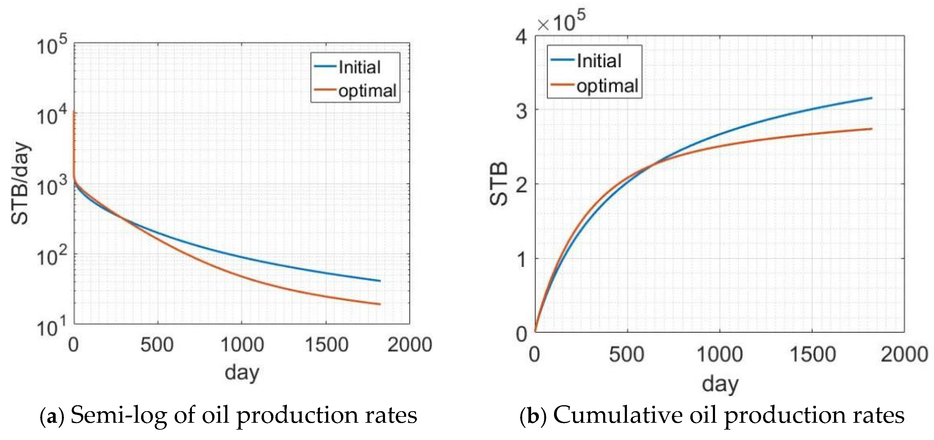
3.1. Fracture Design Optimization

In this case, it assumes the maximum principal stress is the vertical stress ${\sigma }_v$. Therefore, all fractures propagate as vertical planes. Young’s modulus $E$ is set to 5000 MPa (sandstone) with a Poisson’s ratio ($\nu$) of 0.25. The horizontal stresses range from ${\sigma }_h=20$ MPa (minimum) to ${\sigma }_H=25$ MPa (maximum). The size of the reservoir is 2000 m $\times$ 1000 m $\times$ 20 m, with a simulation grid of $200\times 100\times 1$ (totaling 20,000 blocks). The natural fracture intensity is 1000/$\mathrm{k}{\mathrm{m}}^2,$ and the center point of the natural fracture is distributed uniformly over the reservoir. Natural fracture lengths follow a log-normal distribution: $\ln \left(L_S\right)\sim N\left(\ln \left(30\right),{0.5}^2\right)$. Given that natural fractures typically exhibit conjugate orientations, this work models their orientation using a Gaussian mixture distribution: ${\theta }_S\sim {\displaystyle \frac{1}{2}}N\left({45}^{\circ },{{15}^{\circ }}^2\right)+{\displaystyle \frac{1}{2}}N\left(-{60}^{\circ },{{15}^{\circ }}^2\right)$, where 0° corresponds to the maximum horizontal stress direction in the x-y plane. The cohesion coefficient ($S_0$) follows a normal distribution $N\left(\mathrm{0.5,0.1}\right)$ MPa; the internal friction factor is sampled from the truncated Gaussian $N\left(\mathrm{0.3,0.05}\right)$ constrained between 0.05 (lower bound) and 0.15 (upper bound). Tensile strength is drawn from $N\left(1, 0.1\right)$ MPa. To account for uncertainties in natural fracture distribution, ten distinct realizations are generated from these distributions. Figure 3 illustrates two representative realizations of the natural fracture distribution generated through this methodology. The rock matrix is assumed to be homogeneous, with porosity and permeability values of 0.2 and 0.01 mD, respectively. Fracture permeability and porosity are defined as 100 D and 0.8, respectively. In all reservoir simulator runs, the well BHP is 3.45 MPa (500 psi), and the starting reservoir pressure is set at 20.68 MPa (3000 psi). The reservoir’s initial water saturation, which is equivalent to irreducible water saturation, is 0.2. The oil price is USD 60/STB and the cost of disposing of the water is USD 2/STB in order to calculate the NPV; the discount rate is 0.05; the cost of fracturing fluid $c_{\mathrm{fluid}}$ is $\mathrm{U}\mathrm{S}\mathrm{D} 30/\mathrm{S}\mathrm{T}\mathrm{B}$; the cost of proppant $c_{\mathrm{prop}}$ is $\mathrm{U}\mathrm{S}\mathrm{D} 40/\mathrm{S}\mathrm{T}\mathrm{B}$ and the cost of pumping is $c_{\mathrm{pump}}$ $\mathrm{U}\mathrm{S}\mathrm{D}5/\mathrm{M}\mathrm{p}\mathrm{a}$; and ${\beta }_1$, ${\beta }_2,$ and ${\beta }_3$ in Equation (12) are equal to 0.001, 0.005, and 1, respectively.

Figure 4 presents a detailed visualization of the complex fracture network generated through multi-stage hydraulic fracturing in a horizontal well within a naturally fractured reservoir, as simulated using the geo-mechanical model. In this representation, purple lines delineate the horizontal well trajectory, constituting the central component of the fracture network. The blue lines indicate inactive natural fractures that remain non-conductive during the hydraulic fracturing process. The red lines denote hydraulically activated fractures, whose propagation and interconnectivity significantly influence fluid flow within the reservoir. Black lines represent hydraulically reactive yet unopened natural fractures with zero aperture, a critical aspect for reservoir simulation. This characteristic is crucial for reservoir simulation, as according to EDFM principles, zero-aperture fractures lose fluid conductivity, resulting in zero fracture-to-fracture transmissibility. These findings advance our understanding of hydraulic fracturing mechanisms in naturally fractured reservoirs and provide essential theoretical foundations for reservoir simulation and productivity forecasting. In the EDFM, the zero aperture elements act as impermeable faults in the reservoir, which is unrealistic. In reality, those fractures can also serve as permeable conduct in the development of the unconventional reservoir. Therefore, this work assumes that if a fracture is reactive but does not open in the geo-mechanical simulation stage, then the fracture aperture is assigned a very small value (${10}^{-6}$ m) to prevent unrealistic impermeable fractures in the reservoir simulation stage. To save computational resources, only half of a multi-stage fractured well system is simulated (Figure 4), and it assumes that the NPV of the whole well is two times the NPV of the half system. The demonstration case employs a simplified five-stage fracturing design, each containing four perforation clusters. This configuration demonstrates the framework’s versatility without limiting its broader applicability. The framework’s flexibility enables it to overcome constraints related to the number of fracturing stages or fractures per stage. The initial length of each perforation is standardized at 5 m, which translates into the length parameter value of the first fracture element in the DDM.

Table 1. An academic overview of the initial bounds of design variables.

Design Variables	Initial	Lower	Upper
Fracture spacing $L_f$ (m)	20	20	100
Stage spacing $L_s$ (m)	70	20	100
Treatment volume $V_t$ (${\mathrm{m}}^3$)	800	200	1200
Treatment pressure $p_t$ ($\mathrm{M}\mathrm{p}\mathrm{a}$)	23.5	21.5	24.5

details the parameter ranges for all initial design variables, establishing a robust basis for subsequent analysis and optimization.

Figure 5 and Figure 6 illustrate the active fracture pattern generated from the geo-mechanical simulator and also show the pressure profiles at 30 days and 5 years generated by the unconventional reservoir simulator using two different realizations of m, and the initial value of the design parameters. A comparative analysis reveals significant variations in active fracture patterns between the two cases, despite identical initial design parameters. These variations stem from inherent uncertainties in natural fracture network distribution and geo-mechanical property variability. A comparative analysis of Figure 5a,c identifies a specific region (blue circle) where activated fractures demonstrate incomplete drainage efficiency. This phenomenon results from hydraulic multi-stage fracturing (HWMHF) processes where some natural fractures slip without significant dilation. These slipping but non-dilating fractures reduce fluid efficiency and may cause unintended fluid loss during operations. During production, these fractures’ minimal apertures limit their contribution to fracture network connectivity and overall productivity, reducing hydrocarbon recovery efficiency. The limited apertures constrain fracture-to-fracture flow within the active system, resulting in incomplete downstream drainage.

In this research, we employed three distinct derivative-free optimization strategies—GA, PSO, and PS—to achieve robust optimization of fracture designs. For GA, the population size was optimized at five to balance genetic diversity and computational efficiency. The generation limit was set to 30 to optimize computational resource utilization. Similarly, the swarm size of PSO was also set to five, with a maximum iteration count of 30, aiming to explore the optimal solution space through collective intelligence. For PS, the initial mesh refinement level was designated as one-tenth of the search spacing, and the maximum iteration limit was set to 30, allowing for precise adjustments in the search direction. Furthermore, a stagnation detection mechanism was integrated into GA, whereby the algorithm terminates if there is no notable improvement in NPV for five consecutive generations, indicating a potential local optimum.

Table 2. The summary of gradient-free optimization algorithms.

Optimization Algorithm	Average NPV ($\mathbf{U}\mathbf{S}\mathbf{D}\times {10}^7$)	Num. of Simulation
GA	1.41	15,000
PSO	1.33	15,000
PS	1.46	250

presents a comprehensive performance comparison of these optimization algorithms for fracture design tasks. Results indicate that the pattern search demonstrates superior computational efficiency and achieves the highest average NPV ($\mathrm{U}\mathrm{S}\mathrm{D}$1.46$\times {10}^7$) among the algorithms. Initial design parameters yield an average NPV of $\mathrm{U}\mathrm{S}\mathrm{D}$1.07$\times {10}^7$, indicating a potential 35% NPV increase through multi-stage fracture optimization. Table 2 shows that PS significantly outperforms the other two derivative-free algorithms. The optimal design parameters obtained with pattern search are $L_f$ = 58.5 m; $L_S$ = 20.25 m; $V_t$ = 836 ${\mathrm{m}}^3$; and $p_t$ = 23.5 MPa, respectively. Figure 7 presents a comparative analysis of the cumulative distribution function (CDF) of robust NPV under initial and optimal design parameters.

Figure 8 and Figure 9 present the geo-mechanical and reservoir simulation results for realizations 1 and 2 using optimal design parameters. Compared to the initial designs, optimal parameters yield more uniformly spaced fractures with more consistent lengths. Optimal designs significantly reduce slipping and non-opening fractures, improving fracturing fluid efficiency and stimulated region drainage compared to initial parameters.

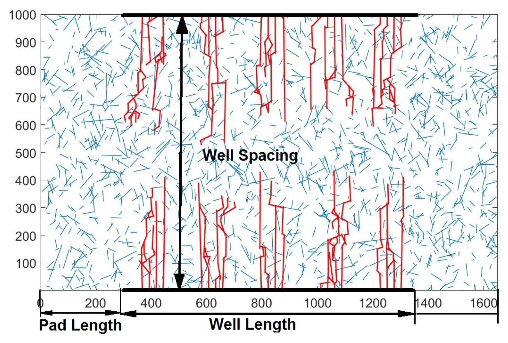
3.2. Well Spacing Optimization

The second case study incorporates well spacing as an additional optimization parameter in robust optimization. Model configurations and cost parameters remain consistent with the previous case, with Equation (17) replacing Equation (10) for the NPV calculation. The land lease cost is set at $c_{\mathrm{lease}}=6\times {10}^6$ $\mathrm{U}\mathrm{S}\mathrm{D}/\mathrm{k}{\mathrm{m}}^2$ for a five-year period. The initial well spacing is set as 1000 m; the initial fracture spacing is set as 20 m; the initial stage spacing is set as 70 m; and the initial treatment volume and pressure are set as 800 m³ and 23.5 MPa, respectively. For simplicity, identical fracture design variables are assumed for both wells. Figure 10 shows the active fracture network from hydraulic fracturing in two horizontal wells using initial design parameters for a specific realization of the random variable m. Subsequently, Figure 11 delves deeper by presenting the pressure profiles at two pivotal time points within the production cycle: after 30 days of production and after the entire production period (spanning 5 years), respectively, thereby revealing the temporal evolution of pressure field dynamics. As shown in Figure 11b, it can be observed that the pressure between the two wells is still relatively high. To be specific, the pressure at the interwell area ($x=900$ m, $y=500$ m) is 850 psi at the end of the production period, corresponding to the producing pressure of 500 psi at the wellbore, which means that the interwell area is not completely drained.

The pattern search algorithm is applied as the optimization algorithm because of its superior performance in the previous example. Figure 12 displays the active fracture network configuration under optimal design parameters, including fracture geometry and well spacing. Compared to initial designs (Figure 10), the optimized parameters increase fracture spacing by 28.5% (680 m vs. 1000 m) while reducing fracture lengths. Figure 13 presents the temporal pressure evolution under optimal designs at 30 days and 5 years. Compared to Figure 11b, the optimal design parameters result in more uniform drainage of the reservoir. The pressure at the inter-well area ($x=900$ m, $y=300$ m) is 595 psi at the end of the production period as opposed to $850$ psi for the corresponding results obtained with the initial values of the design parameters. The optimized parameters are: $L_{\mathrm{spacing}}$ = 685 m; $L_f$ = 60.5 m; $L_S$ = 21.5 m; $V_t$ = 650 m³; and $p_t$ = 22 MPa.

Figure 14 compares production performance between initial and optimized designs using semi-log plots of production rate and cumulative oil production. The initial HWMHF designs showed 24.3% higher cumulative production than optimized configurations, primarily due to larger drainage areas. With this optimal well spacing, the operator can save the cost of leasing land, and fracture tips propagated from each well are not too close, so there is not too much interference between these two wells. This observation is reasonable since the initial fracturing design has a larger drainage area than that obtained for the optimal design case because of the high leasing cost. The expected NPV of the initial multi-stage fracturing design is $\mathrm{U}\mathrm{S}\mathrm{D}$1.38$\times {10}^6,$ whereas the optimal design gives an average NPV equal to $\mathrm{U}\mathrm{S}\mathrm{D}$2.81$\times {10}^6$. Thus, by using the optimal design fracturing parameters to conduct the HWMHF, the operator can achieve a 102.4% increase in terms of the expected NPV (average NPV) of robust optimization. Figure 15 demonstrates the enhanced economic reliability through CDF comparison of robust NPV between initial and optimized designs.

4. Conclusions

This work proposes a novel workflow to maximize the HWMHF design and well spacing in an unconventional naturally fractured oil reservoir with geological and geo-mechanical uncertainties. Two numerical cases are designed to validate the viability of this workflow. It can be concluded as follows:

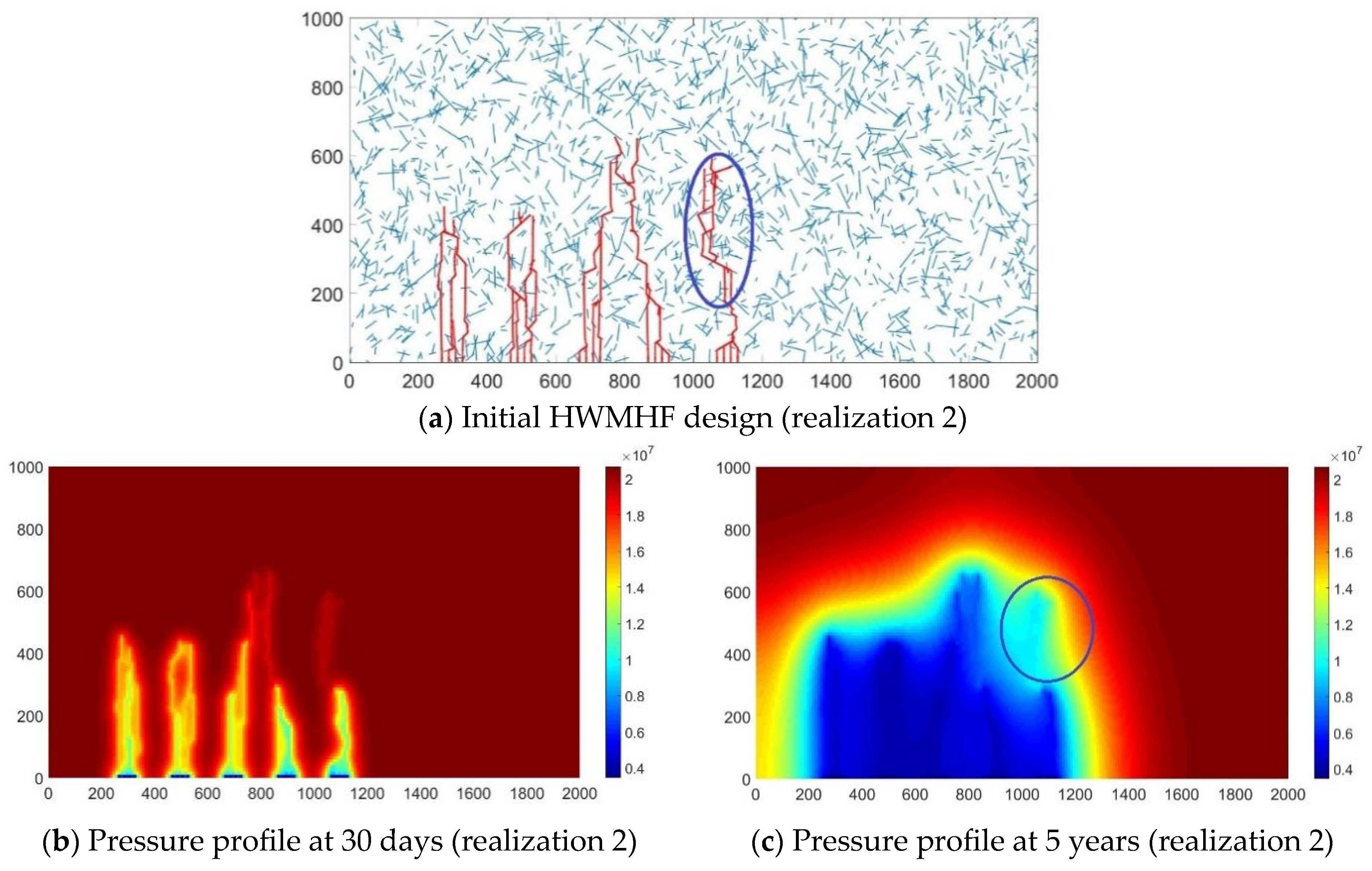
• Basic geo-mechanical principles and HF-NF interactions can be considered in the fracture propagation process, thus creating complex fracture patterns when using DDM. EDFM can be used to explicitly model multi-phase flow in the complex fracture network. HWMHF design and well spacing can be optimized effectively in naturally fractured oil reservoirs by combining the DDM and EDFM.
• Based on the work, oil and gas scientists can find the optimal strategy to develop unconventional resources. This will encourage them to make greater contributions to the oil and gas industry.
• Considering the uncertainties in the natural fracture location, length, and orientation, robust optimization is necessary, and the natural fracture patterns can be sampled from Gaussian distributions. When optimizing HWMHF design and well spacing, the objective function can be defined as the expected comprehensive NPV, which includes the drilling cost, fracturing cost, production revenue, and leasing cost.
• As for the first case in optimizing fracture spacing, stage spacing, treatment pressure, and treatment volume, compared to PSO and GA, the pattern search algorithm yields the best performance in terms of the maximum expected NPV and the computational cost. Compared to the initial guess, the pattern search algorithms improve the average comprehensive NPV by 35$\%,$ with only $250$ forward simulation runs.
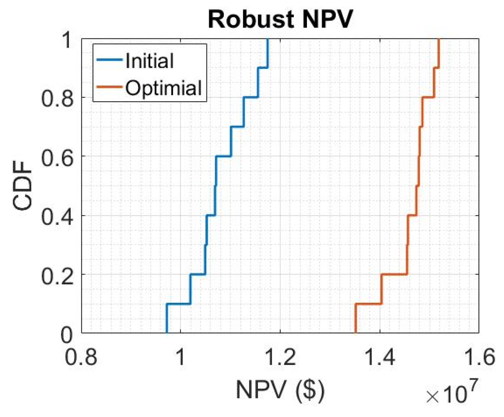
• As for the second case with well spacing added, the estimated optimal design parameters obtained from robust optimization give an average comprehensive NPV equal to $\mathrm{U}\mathrm{S}\mathrm{D}$2.81$\times {10}^6$, which is 102.4$\%$ higher than the average comprehensive NPV ($\mathrm{U}\mathrm{S}\mathrm{D}$1.38$\times {10}^6$) obtained with the initial design parameters.
• The future work will incorporate real field production and microseismic data to validate and calibrate the simulation models. Additionally, extending the optimization framework to multi-well pads with interference modeling will be applied in the field-scale applications.

References

1. Zoback, M.D. Reservoir Geomechanics; Cambridge University Press: Cambridge, UK, 2010. [Google Scholar]
2. Zoback, M.D.; Kohli, A.H. Unconventional Reservoir Geomechanics; Cambridge University Press: Cambridge, UK, 2019. [Google Scholar]
3. Zou, J.; Chen, W.; Yang, D.; Yu, H.; Yuan, L. Complex hydraulic-fracture-network propagation in a naturally fractured reservoir. Comput. Geotech. 2021, 135, 104165. [Google Scholar] [CrossRef]
4. Hekmatnejad, A.; Crespin, B.; Pan, P.Z.; Emery, X.; Mancilla, F.; Morales, M.; Seyedrahimi-Niaraq, M.; Schachter, P.; Gonzalez, R. A hybrid approach to predict hang-up frequency in real scale block cave mining at El Teniente mine, Chile. Tunn. Undergr. Space Technol. 2021, 118, 104160. [Google Scholar] [CrossRef]
5. Fossen, H. Structural Geology; Cambridge University Press: Cambridge, UK, 2016. [Google Scholar]
6. Mack, M.G.; Elbel, J.L.; Piggott, A.R. Numerical representation of multilayer hydraulic fracturing. In Proceedings of the 33th US Symposium on Rock Mechanics (USRMS), Santa Fe, NM, USA, 3 June 1992. ARMA-92-0657. [Google Scholar]
7. Xu, W.; Le Calvez, J.H.; Thiercelin, M.J. Characterization of hydraulically-induced fracture network using treatment and microseismic data in a tight-gas sand formation: A geomechanical approach. In Proceedings of the SPE Tight Gas Completions Conference, San Antonio, TX, USA, 15 June 2009. SPE 119881. [Google Scholar]
8. Dahi-Taleghani, A.; Olson, J.E. Numerical modeling of multistranded-hydraulic-fracture propagation: Accounting for the interaction between induced and natural fractures. SPE J. 2011, 16, 575–581. [Google Scholar] [CrossRef]
9. Wu, K.; Olson, J.E. Simultaneous multifracture treatments: Fully coupled fluid flow and fracture mechanics for horizontal wells. SPE J. 2015, 20, 337–346. [Google Scholar] [CrossRef]
10. Warren, J.; Root, P.J. The behavior of naturally fractured reservoirs. SPE J. 1963, 3, 245–255. [Google Scholar] [CrossRef]
11. Pruess, K.; Narasimhan, T. A practical method for modeling fluid and heat flow in fractured porous media. SPE J. 1982, 22, 14–26. [Google Scholar] [CrossRef]
12. Moinfar, A.; Narr, W.; Hui, M.-H.; Mallison, B.T.; Lee, S.H. Comparison of discrete fracture and dual-permeability models for multiphase flow in naturally fractured reservoirs. In Proceedings of the SPE Reservoir Simulation Symposium, The Woodlands, TX, USA, 21 February 2011. SPE 142295. [Google Scholar]
13. Wu, Y.-S.; Pruess, K. A multiple-porosity method for simulation of naturally fractured petroleum reservoirs. SPE J. 1986, 26, 327–336. [Google Scholar] [CrossRef]
14. Li, L.; Lee, S.H. Efficient field-scale simulation for black oil in a naturally fractured reservoir via discrete fracture networks and homogenized media. SPE J. 2008, 13, 295–303. [Google Scholar] [CrossRef]
15. Moinfar, A.; Varavei, A.; Sepehrnoori, K.; Johns, R.T. Development of a novel and computationally-efficient discrete-fracture model to study IOR processes in naturally fractured reservoirs. In Proceedings of the SPE Improved Oil Recovery Symposium, Tulsa, OK, USA, 14 April 2012. SPE 154263. [Google Scholar]
16. Brouwer, D.R.; Nævdal, G.; Jansen, J.D.; Vefring, E.H.; van Kruijsdijk, C.P.J.W. Improved reservoir management through optimal control and continuous model updating. In Proceedings of the SPE Annual Technical Conference and Exhibition, Houston, TX, USA, 26–29 September 2004. SPE 90149. [Google Scholar]
17. Jansen, J.; Brouwer, D.; Naevdal, G.; van Kruijsdijk, C. Closed-loop reservoir management. First Break 2005, 23, 43–48. [Google Scholar] [CrossRef]
18. Chen, C.; Li, G.; Reynolds, A. Robust constrained optimization of short-and long-term net present value for closed-loop reservoir management. SPE J. 2012, 17, 849–864. [Google Scholar] [CrossRef]
19. Jansen, J.D. Adjoint-based optimization of multi-phase flow through porous media. Comput. Fluids 2011, 46, 40–51. [Google Scholar] [CrossRef]
20. Chen, Y.; Oliver, D.S.; Zhang, D. Efficient ensemble-based closed-loop production optimization. SPE J. 2009, 14, 634–645. [Google Scholar] [CrossRef]
21. Chen, B.; Reynolds, A.C. Ensemble-based optimization of the water-alternating-gas-injection process. SPE J. 2016, 21, 786–798. [Google Scholar] [CrossRef]
22. Shirangi, M.G.; Durlofsky, L.J. Closed-loop field development under uncertainty by use of optimization with sample validation. SPE J. 2015, 20, 908–922. [Google Scholar] [CrossRef]
23. Liu, Z.; Forouzanfar, F. Ensemble clustering for efficient robust optimization of naturally fractured reservoirs. Comput. Geosci. 2018, 22, 283–296. [Google Scholar] [CrossRef]
24. Liu, Z.; Reynolds, A.C. An SQP-Filter algorithm with an improved stochastic gradient for robust life-cycle optimization problems with nonlinear constraints. In Proceedings of the SPE Reservoir Simulation Conference, Galveston, TX, USA, 29 March 2019. SPE 193898. [Google Scholar]
25. Fonseca, R.; Stordal, A.; Leeuwenburgh, O.; Van den Hof, P.; Jansen, J. Robust ensemble-based multi-objective optimization. In Proceedings of the ECMOR XIV-14th European Conference on the Mathematics of Oil Recovery, Catania, Italy, 8–11 September 2014; European Association of Geoscientists & Engineers: Bunnik, The Netherlands, 2014; Volume 2014, pp. 1–14. [Google Scholar]
26. Liu, X.; Reynolds, A.C. Multiobjective optimization for maximizing expectation and minimizing uncertainty or risk with application to optimal well control. In Proceedings of the SPE Reservoir Simulation Symposium, Houston, TX, USA, 23 February 2015. SPE 173249. [Google Scholar]
27. Wilson, K.C.; Durlofsky, L.J. Optimization of shale gas field development using direct search techniques and reduced-physics models. J. Pet. Sci. Eng. 2013, 108, 304–315. [Google Scholar] [CrossRef]
28. Ma, X.; Gildin, E.; Plaksina, T. Efficient optimization framework for integrated placement of horizontal wells and hydraulic fracture stages in unconventional gas reservoirs. J. Unconv. Oil Gas Resour. 2015, 9, 1–17. [Google Scholar] [CrossRef]
29. Li, J.; Gong, B.; Wang, H. Mixed integer simulation optimization for optimal hydraulic fracturing and production of shale gas fields. Eng. Optim. 2016, 48, 1378–1400. [Google Scholar] [CrossRef]
30. Wang, S.; Chen, S. Integrated well placement and fracture design optimization for multi-well pad development in tight oil reservoirs. Comput. Geosci. 2019, 23, 471–493. [Google Scholar] [CrossRef]
31. Wang, L.; Yao, Y.; Zhao, G.; Adenutsi, C.D.; Wang, W.; Lai, F. A hybrid surrogate-assisted integrated optimization of horizontal well spacing and hydraulic fracture stage placement in naturally fractured shale gas reservoir. J. Pet. Sci. Eng. 2022, 216, 110842. [Google Scholar] [CrossRef]
32. Yao, J.; Li, Z.; Liu, L.; Fan, W.; Zhang, M.; Zhang, K. Optimization of fracturing parameters by modified variable-length particle-swarm optimization in shale-gas reservoir. SPE J. 2021, 26, 1032–1049. [Google Scholar] [CrossRef]
33. Li, W.; Zhang, T.; Liu, X.; Dong, Z.; Dong, G.; Qian, S.; Zhang, T. Machine learning-based fracturing parameter optimization for horizontal wells in Panke field shale oil. Sci. Rep. 2024, 14, 6046. [Google Scholar] [CrossRef]
34. Lu, C.; Jiang, H.; Yang, J.; Wang, Z.; Zhang, M.; Li, J. Shale oil production prediction and fracturing optimization based on machine learning. J. Pet. Sci. Eng. 2022, 217, 110900. [Google Scholar] [CrossRef]
35. Zhang, H.; Sheng, J.J. Complex fracture network simulation and optimization in naturally fractured shale reservoir based on modified neural network algorithm. J. Nat. Gas Sci. Eng. 2021, 95, 104232. [Google Scholar] [CrossRef]
36. Gidley, J.L. Recent Advances in Hydraulic Fracturing; SPE Monograph Series; Society of Petroleum Engineers: Richardson, TX, USA, 1989; Volume 12. [Google Scholar]
37. Sih, G.C. On the crack extension in plates under plane loading and transverse shear. J. Fluids Eng. 1963, 85, 462–468. [Google Scholar]
38. Lu, R.; Forouzanfar, F.; Reynolds, A.C. An efficient adaptive algorithm for robust control optimization using StoSAG. J. Pet. Sci. Eng. 2017, 159, 314–330. [Google Scholar] [CrossRef]
39. Liu, Z.; Forouzanfar, F.; Zhao, Y. Comparison of SQP and AL algorithms for deterministic constrained production optimization of hydrocarbon reservoirs. J. Pet. Sci. Eng. 2018, 171, 542–557. [Google Scholar] [CrossRef]
40. Wu, K.; Olson, J.E. Numerical investigation of complex hydraulic-fracture development in naturally fractured reservoirs. SPE Prod. Oper. 2016, 31, 300–309. [Google Scholar] [CrossRef]
41. Crouch, S.L. Solution of plane elasticity problems by the displacement discontinuity method. I. infinite body solution. Int. J. Numer. Methods Eng. 1976, 10, 301–343. [Google Scholar] [CrossRef]
42. Crouch, A.M.; Starfield, R.F.J. Boundary Element Methods in Solid Mechanics; McGraw-Hill: London, UK, 1983; Volume 17. [Google Scholar]
43. Olson, J.E. Predicting fracture swarms—The influence of subcritical crack growth and the crack-tip process zone on joint spacing in rock. Geol. Soc. Lond. Spec. Publ. 2004, 231, 73–88. [Google Scholar] [CrossRef]
44. Kaiser, M.J. A survey of drilling cost and complexity estimation models. Int. J. Pet. Sci. Technol. 2007, 1, 1–22. [Google Scholar]
45. Mayerhofer, M.J.; Lolon, E.; Warpinski, N.R.; Cipolla, C.L.; Walser, D.W.; Rightmire, C.M. What is stimulated reservoir volume? SPE Prod. Oper. 2010, 25, 89–98. [Google Scholar] [CrossRef]
46. Mettam, G.R.; Adams, L.B. How to Prepare an Electronic Version of Your Article; Jones, B.S., Smith, R.Z., Eds.; Introduction to the Electronic Age; E-Publishing Inc.: New York, NY, USA, 2023; pp. 281–304. [Google Scholar]
Figure 1. Illustration of well spacing and well lateral length.
Processes 13 01920 g001
Figure 2. Workflow for the robust HWMHF design optimization.
Processes 13 01920 g002
Figure 3. Two realizations of natural fracture distribution.
Processes 13 01920 g003
Figure 4. The sketch of the hydraulic fractured well in the naturally fractured reservoir (Blue lines: natural fractures; Red lines: hydraulic fractures).
Processes 13 01920 g004
Figure 5. Geo-mechanical and reservoir simulation results for realization 1 with the initial design parameters.
Processes 13 01920 g005
Figure 6. Geo-mechanical and reservoir simulation results for realization 2 with the initial (blue circle: activated fractures demonstrate incomplete drainage efficiency).
Processes 13 01920 g006
Figure 7. CDF of robust NPV with Fracture optimization initial and optimal design.
Processes 13 01920 g007
Figure 8. Geo-mechanical and reservoir simulation results for realization 1 with the optimal design parameters.
Processes 13 01920 g008
Figure 9. Geo-mechanical and reservoir simulation results for realization 2 with the optimal design parameters.
Processes 13 01920 g009
Figure 10. Fracture pattern for the case with the initial design variables.
Processes 13 01920 g010
Figure 11. Pressure profile for the case with the initial design variables.
Processes 13 01920 g011
Figure 12. Fracture pattern for the case with the optimal design variables.
Processes 13 01920 g012
Figure 13. Pressure profile for the case with the optimal design variables.
Processes 13 01920 g013
Figure 14. Comparison of oil production and cumulative production rates with initial (blue) and optimal (orange) fracture designs.
Processes 13 01920 g014
Figure 15. CDF of robust NPV with well optimization initial and optimal designs.
Processes 13 01920 g015