Statistical Analysis of Temperature Sensors Applied to a Biological Material Transport System: Challenges, Discrepancies, and a Proposed Monitoring Methodology

Abstract

Conventional methods for transporting biological materials typically use dry ice or ice for preservation but often overlook important aspects of temperature monitoring and metrological control. These methods generally do not include temperature sensors to track the thermal conditions of the materials during transport, nor do they apply essential metrological practices such as regular sensor calibration and stability checks. This lack of precise monitoring poses significant risks to the integrity of temperature-sensitive biological materials. This study presents a statistical analysis of DS18B20 digital temperature sensors used in an experimental refrigeration system based on thermoelectric modules. The aim was to verify sensor consistency and investigate sources of measurement error. The research was motivated by a prior phase of study, which revealed significant discrepancies of approximately 3 °C between experimental temperature data and numerical simulations. To investigate a potential cause, we conducted a case study analyzing measurements from three identical temperature sensors (same model, brand, and manufacturer). Statistical analyses included ANOVA (analysis of variance) and Tukey’s test with a 95% confidence interval. Since the data did not follow a normal distribution (p-value < 0.05), non-parametric methods such as the Kruskal–Wallis and Levene’s procedures were also applied. The results showed that all sensors recorded statistically significant different temperature values (p-value < 0.05). Although experimental conditions were kept consistent, temperature differences of up to 0.37 °C were observed between sensors. This finding demonstrates an inherent inter-sensor variability that, while within manufacturer specifications, represents a source of systematic error that can contribute to larger discrepancies in complex systems, highlighting the need for individual calibration.

1. Introduction

The transportation of biological materials such as organs, blood, and temperature-sensitive medications requires effective cooling systems to maintain their integrity and therapeutic value. It is essential to keep the temperature within specific ranges to prevent biochemical degradation, slow down cellular metabolism, and preserve the material’s viability until it is used [1]. However, challenges remain, including maintaining stable temperatures over long periods, improving energy efficiency, and ensuring the reliability of thermal monitoring sensors, which limit the performance of conventional systems.

Developing new portable refrigeration technologies has become an important area of research, with direct benefits for the safety and efficiency of transporting biological materials [2]. Additionally, controlling ice formation by using antifreeze protein solutions and sodium chloride has significantly slowed ice growth in refrigeration systems, helping to maintain the thermal stability needed to preserve the viability of biological materials [3].

Recent studies have demonstrated that the DS18B20 temperature sensor is effective for precise thermal monitoring in various applications. Elyyounsi and Kalashnikov [4] found it comparable to Pt100 sensors in controlled environments, showing minimal bias (0.05 °C) and variation (±0.08 °C). This supports its use as a low-cost alternative in low-airflow conditions. Koritsoglou et al. [5] showed its suitability for freezer automation by applying linear regression calibration, achieving results aligned with EN12830 standards [6] and ensuring compliance for food and pharmaceutical storage. In biomedical settings, Siswoyo [7] identified the DS18B20 as the most accurate sensor among DHT22 and LM35 in incubator simulations, with a deviation of ±0.3 °C and a response time of 2–3 s, recommending it for critical applications. Nie, Cheng, and Dai [8] validated its use in energy systems, demonstrating reliable conductor temperature measurements in high-voltage transmission lines, which supports dynamic capacity management. Overall, the DS18B20 proves to be a versatile, reliable, and cost-effective sensor for thermal monitoring across diverse technical fields.

Refrigerated devices used for transporting biological materials typically rely on dry ice or phase change material (PCM) packs or canisters as cooling methods. The transport of biological materials, especially organs, is usually carried out in thermal containers made of expanded polyethylene combined with these refrigeration techniques [9]. The main objective is to maintain the material in a hypothermic state to ensure proper preservation. The operating temperature of the system—from the donor’s departure to the recipient’s arrival—depends entirely on the type of biological material being transported. To reduce organ metabolism in the absence of blood flow, the preservation temperature in the hypothermic state must be kept between 0 and 4 °C, preventing functional damage during transplantation [10].

In the pharmaceutical industry, products such as insulin and vaccines are classified as thermolabile materials, meaning they are highly sensitive to temperature changes. These products are generally required to be stored within a temperature range of 2 to 8 °C, although in exceptional cases, temperatures below 0 °C may be specified (Crf-SP, 2019). Exposure outside these ranges can cause degradation and eventual disposal of the materials. As demonstrated by Hien and Thanh [11], effective cold chain management is critical to maintaining the quality and safety of medications like vaccines. Selecting suppliers who comply with strict temperature requirements is also essential for transporting other biological materials.

Recent research has focused on developing portable cooling systems based on thermoelectric devices for transporting biological materials and general refrigeration. Lin et al. [12] highlight several advantages of these devices compared to traditional compressor-based refrigeration systems: they are compact, operate silently, consume less electricity, and are environmentally friendly. Their study explored ways to improve thermoelectric module performance by optimizing the heat exchangers attached to the cold and hot sides. The results showed that thermal performance improves when the modules are paired with finned aluminum heat exchangers and operated at 8V, starting from an ambient temperature of 25 °C.

Daou et al. [13] developed a portable device for monitoring and controlling the temperature of insulin pens. The device features two internal chambers for storing new and used pens, along with temperature and presence sensors that transmit data to a web server. After 36 h of testing in various environments, the authors concluded that the device effectively monitored and controlled temperature and detected the presence of insulin pens in both chambers. Their prototype also includes an app that notifies users about electric current parameters, battery charge levels, and whether reservoir temperatures remain within established standards.

During the COVID-19 pandemic, Ivanov et al. [14] proposed a solution for low-temperature vaccine storage. Their prototype is a cylindrical, thermally insulated container designed to store pharmaceuticals, equipped with temperature and humidity sensors that collect data and transmit it to a datalogger. Similarly, Novais et al. [15] developed an analogous system to facilitate medicine distribution in remote areas. Their system is powered by solar energy via photovoltaic panels, with part of the energy stored in lead–acid batteries. During validation tests, the device consumed approximately 3.5 W from the photovoltaic panel, maintaining a temperature range of 2 to 8 °C with a coefficient of performance (COP) of 0.004.

Expanding the application of this technology to various medical fields, Taspinar and Isik [16] studied refrigerated organ transport, validating their results using an animal kidney at ambient temperatures of 25 °C, 30 °C, 35 °C, and 40 °C. They observed that at 25 °C, the internal temperature of the reservoir reached −5 °C in approximately 120 s. For higher ambient temperatures, it took between 180 and 600 s. The authors emphasized that the system can be adjusted to maintain different internal temperatures and includes visual and audible alerts for excessive cooling or heating.

Umchid et al. [17] proposed a refrigerated blood transport system using PID control to regulate temperature. After completing experiments, they found that the average temperature readings from five Type K sensors inside the container differed slightly from those recorded by the datalogger. Variations ranged from 0 to 0.15 °C, with an error of ±10.984%, a standard deviation of 0.496 °C, and a measurement uncertainty of 0.109 °C. The authors attributed these discrepancies to the placement of the sensors.

In Abderezzak et al. [18], a new configuration for refrigeration was introduced using thermoelectric modules coupled with heat exchangers. Their experiments revealed temperature fluctuations from 0.5 to 3.8 °C on the cold side. These variations were attributed to forced convection caused by airflow generated by an internal fan, resulting in inaccurate temperature sensor readings. However, it was not confirmed whether the issue was due to the sensors themselves or caused by forced convection, as no variance analysis was conducted. Experimental validation through comparative analysis has long been a crucial tool for assessing the feasibility of numerical models in various engineering fields. This includes refrigeration systems [19,20], heat and mass transfer studies [21,22], and computational fluid dynamics (CFD) analyses [23,24], among others.

To date, few studies have addressed a metrological or statistical analysis of the temperature sensors used during the experimental phase of refrigeration systems with thermoelectric devices. Additionally, there has been little evaluation of the reliability of the collected data, the need for sensor calibration, or methods to monitor sensor stability. In previous works, the data are generally assumed to follow a normal distribution, and the sensors are considered to provide consistent readings without variation. This study offers an original contribution by employing a robust and easy-to-apply statistical methodology to evaluate the reliability of DS18B20 temperature sensors. This investigation was directly motivated by a previously observed variation of approximately 3 °C in temperature readings during the validation of a numerical simulation of a thermoelectric cooling system. Unlike most of the works that assume uniformity in sensor readings, the results obtained here show statistically significant discrepancies between identical sensors, even under controlled conditions. The main contributions of this work include:

✓

The application of parametric (ANOVA, Tukey test) and non-parametric (Kruskal–Wallis, Levene’s, and Shapiro–Wilk statistical methods to assess data normality, identify differences between sensors, and demonstrate the need for individual calibration.

✓

Statistical verification of significant variations between sensors of the same model and specification.

✓

Experimental identification of the influence of systematic errors (bias) in critical applications.

✓

Proposal of a standardized, practical, and replicable methodology for validating temperature sensors, based on periodic calibration, statistical verification, and use of redundant sensors, applicable in laboratory and field environments.

2. Experimental Analysis

This section outlines experimental data collected from temperature sensors installed in a cooling prototype based on a thermoelectric module. The study was motivated by the hypothesis that the temperature sensors used (model DS18B20) might not provide the required metrological reliability. This concern arose due to an observed variation of approximately 3 °C in the temperature readings on the cold side of the thermoelectric module during the validation of a previously reported numerical simulation. The details of this simulation model (including geometry, boundary conditions, and its key results, such as the predicted temperature distribution) were reported in a previous study [9]. That earlier work highlighted the observed discrepancy, motivating the present investigation focused on the metrological reliability of the sensors as a potential contributing factor to such differences.

To address this issue, a statistical analysis was conducted using ANOVA and Tukey tests [25,26], involving three DS18B20 sensors of the same brand and manufacturer, with a confidence level of 95%.

The DS18B20 is a fully digital temperature sensor that converts temperature directly into digital data through its integrated analog-to-digital converter. It transmits temperature readings via a 1-Wire digital communication protocol. Unlike analog sensors, which require an external analog-to-digital converter, the DS18B20 performs this conversion internally and offers programmable resolution from 9-bit to 12-bit precision.

In this study, the DS18B20 sensors operated within a temperature range of −55 °C to +125 °C, with a manufacturer-specified accuracy of ±0.5 °C between −10 °C and +85 °C, and ±2 °C outside this range. The sensors provide programmable resolution from 9 bit (0.5 °C) to 12 bit (0.0625 °C). The maximum 12-bit resolution (0.0625 °C) was employed in the experiments. It is important to note that resolution and accuracy represent distinct specifications: resolution determines the smallest detectable temperature change for a single sensor, while accuracy reflects the maximum expected deviation between different sensor units due to manufacturing variations in electronic components such as regulators and op-amps. Using the 1-Wire interface, multiple sensors can communicate over a single data line. The typical thermal response time of the sensors in still air is 750 ms.

Power was supplied externally by the Arduino UNO’s 5V output, with the sensors operating within a voltage range of 3.0 V to 5.5 V. These specifications are significant given the observed temperature discrepancies of up to 3 °C between identical sensors under controlled conditions. This indicates that actual performance may deviate from manufacturer specifications if proper calibration is not conducted.

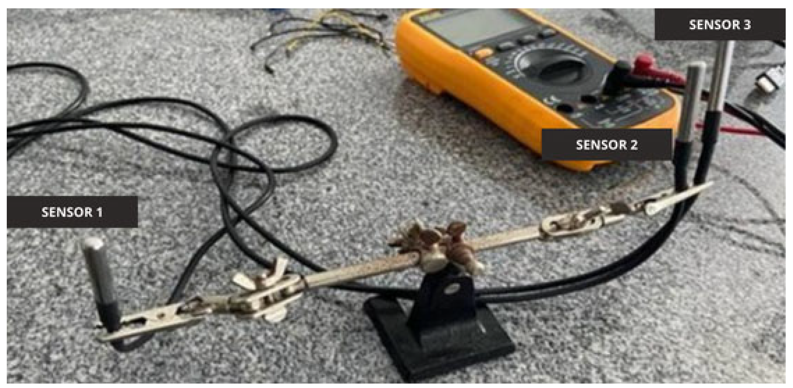
2.1. Description of the Experimental Setup

The experiment was conducted in a carefully controlled environment to minimize external interference in the measurements and validate the hypothesis. Three identical, uncalibrated sensors of the same model and manufacturer were chosen. These sensors were positioned close together (Figure 1) to assess whether their readings showed significant differences.

The experiment took place in a laboratory with controlled ambient temperature (20 ± 1 °C) and minimal air circulation to ensure uniform conditions for all sensors. Although no separate calibrated reference instrument was used as control, the primary objective of this experiment was to assess the intrinsic variability and statistical consistency among identical, uncalibrated sensors. Therefore, a direct comparison methodology was chosen, following established practices for temperature sensor evaluation reported in the literature [5,7,27] in order to isolate this specific source of potential error.

The sensors were connected directly to an Arduino UNO prototyping platform, which handled data acquisition, storage, and display. Temperature data were collected using the Arduino UNO microcontroller interfaced with DS18B20 digital temperature sensors. The Arduino was programmed via the Arduino IDE, utilizing the One Wire library for communication and the Dallas Temperature library for sensor-specific functions. Each DS18B20 sensor was connected to the Arduino with a 4.7 kΩ pull-up resistor between the data line and VCC (5 V), as recommended by the manufacturer. The sensors were identified by their unique 64-bit ROM codes, allowing simultaneous readings from multiple sensors on the same digital pin. Data were transmitted in real time via serial communication (baud rate: 9600) to a connected computer, where they were logged using Microsoft Excel. Time stamps were recorded with each temperature reading to enable temporal analysis of thermal behavior. Initial data processing was performed in Excel, and further statistical analysis was conducted using the R software platform, version 4.3.1. [28].

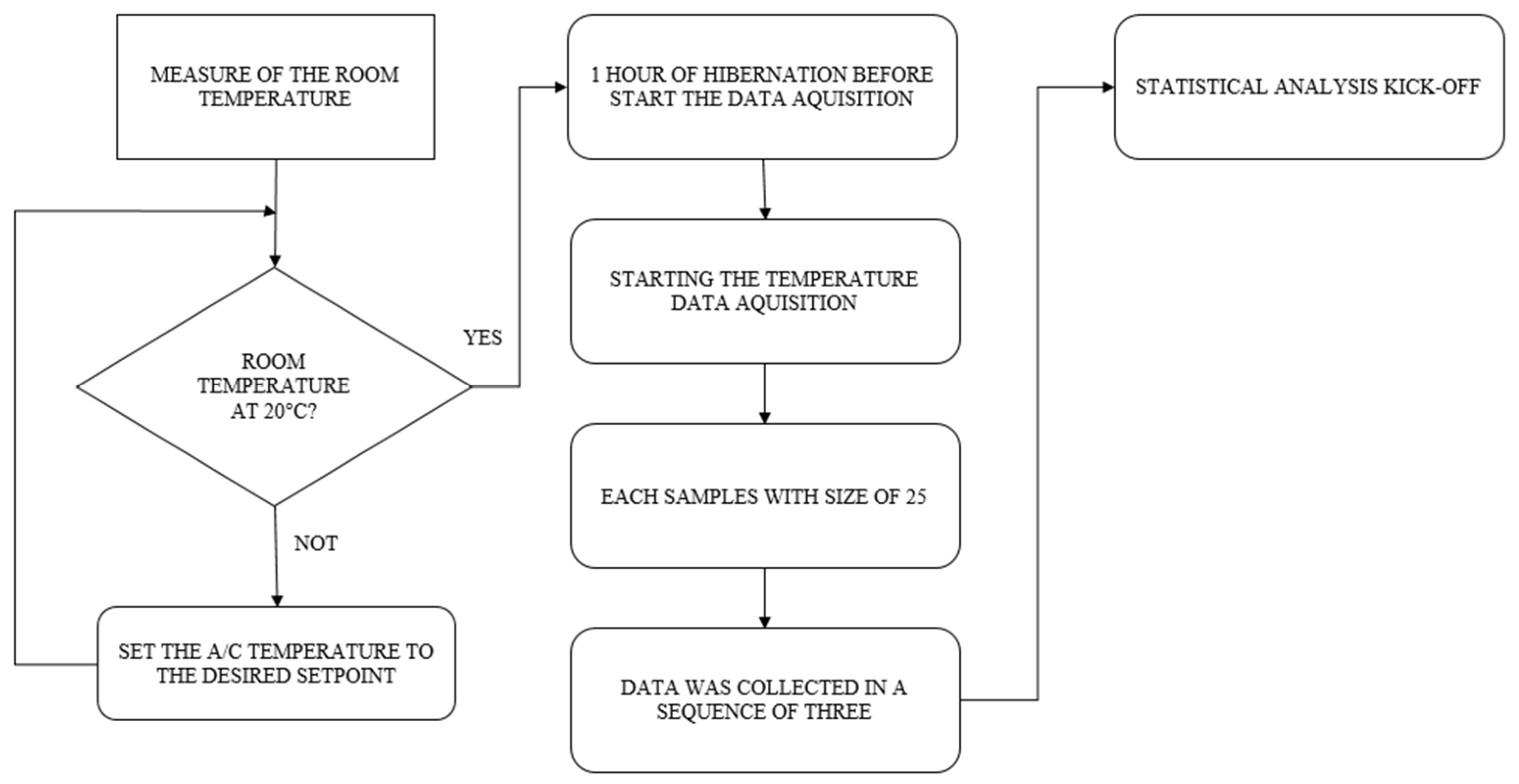
2.2. Experimental Procedure

The first step was to measure the laboratory’s ambient temperature, which was maintained at approximately 20 °C. An additional stabilization period of one hour was allowed before beginning data collection for the different samples. The flowchart in Figure 2 illustrates the data collection procedure used in this study.

After the stabilization period, data acquisition began. Three samples were collected on three different days from the three temperature sensors. Data were collected simultaneously on separate days to allow enough time for the ambient temperature to return to its original equilibrium, thereby preventing compromise in the sample values.

3. Statistical Analysis

This section presents the statistical methodology employed to analyze the collected data, utilizing both parametric and non-parametric tests, as summarized in the flowchart shown in Figure 3. The first step involved assessing the normality of each randomly selected sample, followed by identifying any potential outliers, and then applying a one-way ANOVA test. If significant differences between population means were detected, the Tukey test was subsequently conducted.

An important consideration is how to handle samples that do not originate from a normally distributed population. In such cases, a non-parametric test is used to evaluate differences between populations, which in this study correspond to the equality of temperatures among the three sensors. The equations for the statistical tests are presented in

Table 1. Statistical test equations.

Equation Name	Equation	Variables	Number
ANOVA (Analysis of Variance)	$F={\displaystyle \frac{M{S}_{between}}{M{S}_{within}}}$	$M{S}_{between}={\displaystyle \frac{S{S}_{between}}{d{f}_{between}}}={\displaystyle \frac{{\sum }_{i=1}^k{n}_i{\left({\overline{x}}_i-\overline{x}\right)}^2}{k-1}}$ $M{S}_{within}={\displaystyle \frac{S{S}_{within}}{d{f}_{within}}}={\displaystyle \frac{{\sum }_{i=1}^k{\sum }_{j=1}^{n_i}{\left(x_{ij}-{\overline{x}}_i\right)}^2}{N-k}}$	(1)
Turkey’s Test	$q={\displaystyle \frac{{\overline{x}}_A-\overline{x}B}{\sqrt{\frac{MSwithin}{n}}}}$		(2)
Critical value for comparison	$HSD=q_{\alpha ,k,df}\cdot \sqrt{{\displaystyle \frac{M{S}_{within}}{n}}}$	$q_{\alpha ,k,df}:$ the studentized range statistic	(3)
Kruskal–Wallis test statistic	$H={\displaystyle \frac{12}{N\left(N+1\right)}}{\displaystyle \sum _{i=1}^k}{\displaystyle \frac{R_i^2}{n_i}}-3\left(N+1\right)$	$N:$ total number of observations $n_i$: number of observations $R_{ij}$: rank of observation $j$ from group $i$ $R_i:$ sum of ranks in group $i$ ${\overline{R}}_i$: the mean rank of group $i$ $\overline{R}$: mean of all ranks	(4)
Levene’s Test	$W={\displaystyle \frac{\left(N-k\right)}{\left(k-1\right)}}{\displaystyle \frac{{\sum }_{i=1}^k{n}_i{\left(Z_{i.}-Z_{..}\right)}^2}{{\sum }_{i=1}^k{\sum }_{j=1}^{n_i}{\left(Z_{ij}-Z_{i.}\right)}^2}}$	$Z_{ij}=\left|X_{ij}-{\overline{X}}_{i.}\right|$ is the absolute deviation from group mean, $Z_{i.}$ is the mean of $Z_{ij}$ for group $i$ and $Z_{..}$ is the overall mean of $Z_{ij}$	(5)

.

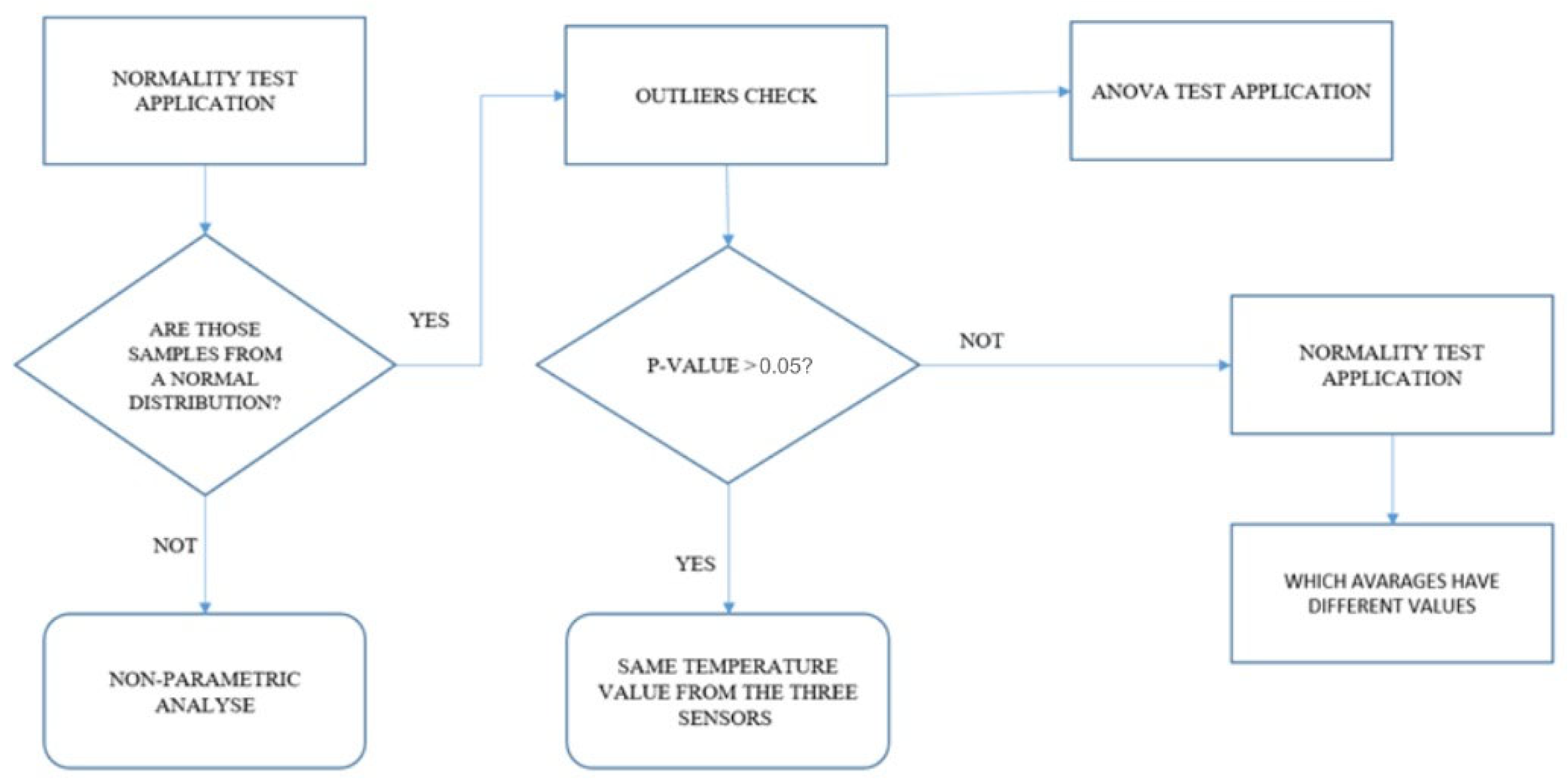
3.1. Parametric Analysis Procedure

A hypothesis test is conducted to verify the normality of the collected samples, which were initially considered as residual distribution patterns rather than raw data. In this analysis, the residuals are assumed not to follow a normal distribution. The error α represents the probability of incorrectly rejecting the null hypothesis of residual normality when the data actually follow or approximate a normal distribution [29]. If the test yields a p-value greater than 0.05, the residuals are considered normally distributed, supporting the non-rejection of the null hypothesis, although Type II errors may still occur. Conversely, rejecting the null hypothesis confirms non-normality [29]. The hypotheses are defined as follows:

H₀: 

The temperatures measured by the three sensors are equal.

H₁: 

At least one sensor records a different temperature.

The Shapiro–Wilk test is used [30] to assess the normality of the samples collected from the three sensors. This test calculates a statistic based on the deviations of the data from the mean and variance. The null hypothesis assumes that the data come from a normally distributed population. If the p-value is less than the significance level (0.05), the null hypothesis is rejected, indicating that the data are not normally distributed [31]. The one-way ANOVA test is a statistical method used to compare the means of two or more populations [26]. It evaluates whether a specific factor (independent variable) has a statistically significant effect on a variable of interest (dependent variable). At this stage, it is essential to clearly define the hypotheses: the null hypothesis (H₀) represents no effect, while the alternative hypothesis (H₁) is accepted only if H₀ is rejected.

Regardless of the test outcome, data analysis may involve:

• Rejecting a true null hypothesis (Type I error).
• Accepting a false null hypothesis (Type II error).

The F-distribution test is applied to statistically assess the equality of variances, ensuring the validity of the analysis when means tend to differ. This test calculates the ratio between two variances; a higher F-value indicates greater data dispersion [26]. If ANOVA detects significant differences, it does not specify which means differ. Therefore, Tukey’s test is used [25,26], which provides high accuracy when group sample sizes are equal. This test compares all pairs of means using Equation (6):

$$HSD=q_{k,g,l,\propto }\sqrt{\left({\displaystyle \frac{QMR}{n}}\right)}$$

(6)

where q (k, g, l, ∝) is the studentized range value (from the q-table) based on the number of treatments and degrees of freedom, n is the number of repetitions per group, and QMR is the mean square error from the ANOVA.

3.2. Non-Parametric Analysis Procedure

The non-parametric Kruskal–Wallis test was applied to determine whether the samples come from normally distributed populations and whether three or more independent groups originate from the same population [19,32]. This test ranks all data in ascending order and computes test statistics based on these ranks. The null hypothesis states that all group medians are equal. If the p-value is less than the chosen significance level (0.05), the null hypothesis is rejected, indicating that at least one group median is different [33].

H₀: 

Temperatures from all three sensors are equal.

H₁: 

At least one sensor records a temperature different from the others.

Levene’s test was applied to verify whether the variances among the three sensors are equal based on the samples [34,35] using the R platform. The hypotheses were:

H₀: 

Sensor variances are equal.

H₁: 

At least one sensor has a different variance.

This test assesses the equality of variances by calculating the group variances and testing the null hypothesis using the absolute or squared differences between observations and their group medians.

4. Analysis and Discussion of Results

This section presents the case study developed using the proposed statistical methodology and highlights the most significant findings.

4.1. Case Study Description

The case study was chosen by comparing the numerical and experimental results of a thermoelectric module-based cooling system prototype designed for preserving biological material, as developed by Roque et al. [9]. Bench tests in that study showed a temperature difference of approximately 3 °C on the cold side of the thermoelectric module. Due to this discrepancy, a statistical analysis of the temperature sensors was performed using ambient temperature data collected in the laboratory where the tests took place. The goal was to confirm or reject the hypothesis stated in Section 3.1.

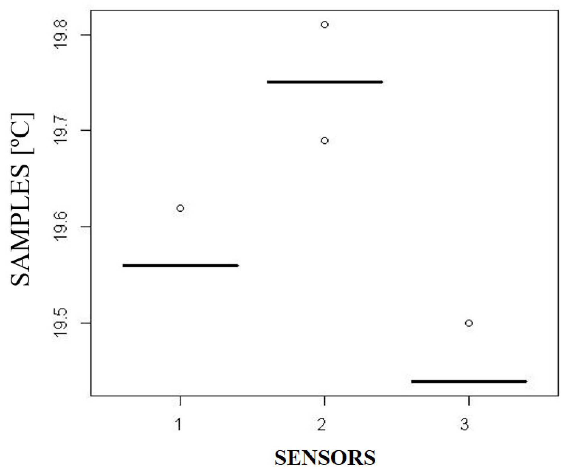
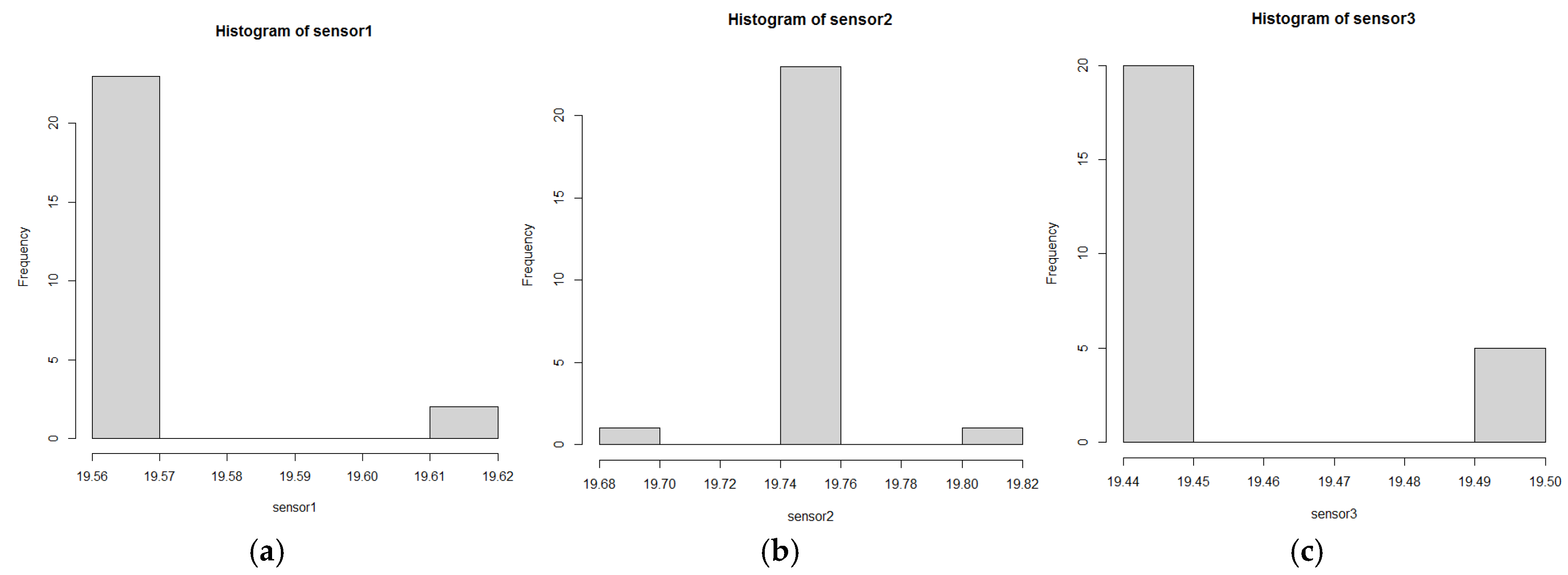
4.2. Measurement Results from the Three Temperature Sensors

Table 2. Ambient temperature data collected from the three sensors in the laboratory.

N° of Samples	S1	S2	S3	N° of Samples	S1	S2	S3
1	19.56	19.75	19.44	14	19.56	19.75	19.44
2	19.62	19.75	19.44	15	19.56	19.75	19.5
3	19.56	19.75	19.44	16	19.56	19.75	19.44
4	19.56	19.75	19.44	17	19.56	19.81	19.5
5	19.56	19.75	19.44	18	19.56	19.75	19.44
6	19.56	19.75	19.44	19	19.56	19.75	19.44
7	19.56	19.75	19.44	20	19.56	19.75	19.44
8	19.56	19.75	19.44	21	19.56	19.75	19.5
9	19.62	19.75	19.44	22	19.56	19.69	19.5
10	19.56	19.75	19.44	23	19.56	19.75	19.44
11	19.56	19.75	19.44	24	19.56	19.75	19.44
12	19.56	19.75	19.44	25	19.56	19.75	19.5
13	19.56	19.75	19.44

displays the experimental data collected from the three temperature sensors (S1, S2 and S3). For each sensor, three separate samples were taken, each sample consisting of 25 measurements.

A boxplot was created to compare the central tendency and variability of each sample, as shown in Figure 4.

Figure 5 illustrates the histograms of temperature readings for Sensors 1, 2, and 3, respectively, allowing for a visual analysis of the frequency distribution of the collected data for each sensor. These histograms reveal distinct characteristics in the temperature distributions of each sensor. An asymmetry in data distribution is observed for Sensors 1 (Figure 5a) and 3 (Figure 5c), with a notable concentration of measurements at specific values, as evidenced by the coincidence of Q1, median, and Q3 values for these sensors.

The concentration in a few temperature steps is directly related to the resolution of the DS18B20 sensor, which operated at 12 bits, resulting in increments of 0.0625 °C. Under stable ambient temperature conditions, such as those present in the laboratory, readings tend to cluster around the discrete values that the sensor is capable of registering. In contrast, Figure 5b, corresponding to Sensor 2, displays a distribution that is closer to symmetry, with most values concentrated between 19.74 °C and 19.76 °C. Although also influenced by the sensor’s resolution, the distribution of Sensor 2 exhibits a slight dispersion around its central value, differing from the more pronounced concentration observed in Sensors 1 and 3.

Further confirming the observations, the non-normal nature of these distributions was later validated by the Shapiro–Wilk test (Section 4.3), attributing some variations to the discretization inherent in the sensor’s analog-to-digital conversion. The visual differences in the histogram shapes and their central peaks hint at sensor variability, which becomes evident given that each sensor shows slightly different distribution patterns despite being of the same model and operating under identical conditions. This variability foreshadows the statistically significant differences in their median readings, quantified in Section 4.3.

Subsequently, the detailed assessment of potential measurement artifacts points out that while the DS18B20 digital sensor converts temperature readings into digital steps, its accuracy range of ±0.5 °C aligns with the observed sensor differences. Therefore, our findings underscore the expectation of performance variation and the necessity for individual sensor calibration in precision-required applications like monitoring temperature-sensitive biological materials.

Lastly, reinforcing the non-normal distribution results, the Shapiro–Wilk test yielded p-values of 3.637 × 10⁻⁹ for Sensor 2, 7.518 × 10⁻¹⁰ for Sensor 1, and 3.217 × 10⁻⁸ for Sensor 3, indicating non-normality at a 95% confidence level. Future work should involve comparing these results with higher-precision temperature measurement systems to verify the non-normal characteristics observed in these digital sensors.

4.3. Parametric and Non-Parametric Statistical Study

Although the boxplots allowed for the visual identification of potential outliers (Figure 4), it was decided not to formally remove them before the subsequent non-parametric analyses. This decision aims to preserve the original integrity of the collected data, especially since non-parametric tests, such as the Kruskal–Wallis test, are more robust to the influence of outliers compared to parametric methods.

In Figure 4, a concentration of values within a narrow range is observed, resulting in the coincidence of the first quartile, the median, and the third quartile. This pattern is also reflected in the histograms presented in Figure 5. Consequently, the Shapiro–Wilk test was performed, and the p-values for each sensor are listed in

Table 3. Results of the Shapiro–Wilk normality test for the samples.

Sensor	p-Value
1	7.518 × 10−10
2	3.637 × 10−9
3	3.21 × 108

.

These p-values clearly indicate that none of the samples come from normally distributed populations, as they are below the 5% significance level. Therefore, it is necessary to use non-parametric statistical methods to determine whether the three sensors provide equivalent temperature measurements.

In non-parametric analysis, where the data do not follow specific probability distribution, the median is the most appropriate measure of central tendency. Similarly, the interquartile range (IQR) is used to describe variability instead of standard deviation [36].

Table 4. Statistical summary of the collected temperature sensor data.

	Sensor 1	Sensor 2	Sensor 3
Minimum Value (°C)	19.56	19.69	19.44
Q1 (°C)	19.56	19.75	19.44
Median (°C)	19.56	19.75	19.44
Q3 (°C)	19.56	19.75	19.44
Maximum Value (°C)	19.62	19.81	19.50

presents the statistical summary for each sample, generated using R [37].

The non-parametric Kruskal–Wallis test was applied [36] to assess the accuracy of the three sensors under the same conditions, as shown in

Table 5. Kruskal–Wallis test result.

Chi-Squared	Degree of Freedom	p-Value
71.262	2	3.354 × 10−16

. The hypotheses tested were:

H₀: 

The temperature readings from the three sensors are equal.

H₁: 

At least one sensor records a different temperature.

Since the p-value is less than 0.05, the null hypothesis was rejected, indicating that at least one sensor provides a significantly different temperature reading. A post hoc test was conducted using the R platform to determine which sensor pairs differ, as shown in

Table 6. p-values for temperature equality between sensors.

	Sensor 1	Sensor 2
Sensor 2	1.5 × 10−11	-
Sensor 3	3.8 × 10−11	3.8 × 10−11

.

While the statistical analysis revealed significant differences between temperature readings from the three DS18B20 sensors (Table 4 and Table 5), it is important to interpret these results in the context of the manufacturer’s specifications. The observed median variations between sensors (peak-to-peak variation of 0.37 °C) fall within the manufacturer’s specified accuracy range of ±0.5 °C for the DS18B20 sensor. This distinction highlights the difference between statistical significance and practical relevance in measurement science.

It is important to distinguish between sensor resolution and accuracy when interpreting these results. Resolution (0.0625 °C at 12-bit in our study) refers to the smallest temperature change a single sensor can detect, while accuracy (±0.5 °C for the DS18B20) represents the maximum deviation from the true temperature value across different sensor units. The observed variations between sensors (peak-to-peak difference of 0.37 °C) exceed the resolution limit but remain within the manufacturer’s specified accuracy range. This indicates that while the differences between sensors are statistically significant and not due to quantization effects, they are consistent with expected manufacturing variations in electronic components such as regulators and op-amps that create built-in offsets unique to each physical sensor.

From a statistical viewpoint, the tests show that the sensors consistently produce different readings compared to each other, with high confidence (p < 0.05). However, from a practical engineering perspective, all sensors operate within their intended design specifications. This finding does not indicate sensor malfunction but rather demonstrates that even properly functioning sensors operating within their accuracy limits can yield consistently different readings when compared directly.

This observation has important implications for applications requiring precise temperature control. In non-critical uses, these differences may be negligible. However, understanding these systematic differences is essential for accurate system calibration, especially in the transport of biological materials and other sensitive processes, particularly when multiple sensors are used within a system or when sensors are replaced over time.

For applications demanding precision beyond the manufacturer’s stated ±0.5 °C accuracy, individual sensor calibration against a traceable reference standard is necessary, regardless of the statistical differences observed between sensors.

All p-values are below 0.05, confirming that each of the three sensors differs statistically, even though the median values vary only in the first decimal place. Despite maintaining consistent experimental conditions, these discrepancies may be due to the lack of calibration of the three sensors. Since systematic errors were unknown, no point-specific correction could be applied. This also helps explain the differences observed between simulated and measured values.

Levene’s Test was conducted using R software, version 4.3.1 to assess the equality of variances among the three sensors,

Table 7. Levene’s test result (center = median).

Degrees of Freedom	F-Value	Pr (>F)
2	1.125	0.3303

:

The null hypothesis was not rejected because the p-value (0.3303) exceeded the significance level of 0.05. Therefore, the population variances of the three sensors are considered statistically equal under the test conditions. This result, together with the significant differences in medians identified by the Kruskal–Wallis test, indicates that the sensors exhibit systematic measurement differences (bias) rather than differences in measurement precision (variance). In other words, each sensor consistently measures at a distinct level, but the variability of measurements around each sensor’s median remains similar.

The validation of an actual variation of up to 0.37 °C between the sensors is, therefore, a central finding. It confirms the hypothesis that motivated this study: that sensor inconsistency is a real and non-negligible source of error in the experimental system. Thus, for future comparisons between experimental data and numerical simulations to be more accurate, the individual calibration of sensors to mitigate this 0.37 °C variation is demonstrated here as an essential methodological procedure.

4.4. Critical Considerations, Limitations and Challenges

The sample size of 25 measurements per sensor was selected based on previous exploratory studies [17,18], which employed sample sizes between 20 and 30 to assess thermal fluctuations in refrigeration systems, balancing detection capability with practical feasibility. The absence of prior calibration in this study was intentional, aiming to analyze the intrinsic variability of identical sensors-a strategy also employed in the literature [19,32] during early-stage non-parametric analyses.

Although the Kruskal–Wallis test is statistically robust and widely accepted for similar applications, it has certain limitations:

• Difficulty in distinguishing systematic errors (e.g., manufacturing defects) from random errors (e.g., thermal noise).
• Limited generalizability, as only three sensors of a single model (DS18B20) were tested.
• Lack of metrological validation of the data acquisition system (Arduino UNO), which may affect measurement resolution.

Compared to studies such as Mobaraki et al. [38], which relied solely on parametric methods (e.g., standard deviation, normal distribution) to reduce uncertainties through averaging across sensors, the present work advances the analysis by identifying non-normality (via Shapiro–Wilk test) and applying non-parametric tests (Kruskal–Wallis and Levene’s). It also includes ANOVA and Tukey’s post hoc tests to compare identical sensors, revealing statistically significant differences even under controlled conditions.

Furthermore, this study explicitly correlates observed discrepancies (up to 3 °C) with the necessity for continuous calibration, a point not addressed by Mobaraki et al. [38], who focused exclusively on static reference-based calibration. Temperature control is essential for maintaining the integrity of biological materials during storage and transport. In the context of cell and tissue preservation, stable temperature is crucial to ensure the quality of laboratory test results involving specimens such as blood and plasma. This was demonstrated by Tanvir et al. [39], who emphasized that proper storage at 4 °C is vital for accurate trace element detection, with temperature fluctuations posing significant risks to sample integrity.

Temperature variations also directly affect enzyme activity and protein stability. Peterson et al. [40] observed that Km values for enzymes tend to increase with temperature, sometimes dramatically, indicating that even moderate temperature rises can substantially alter substrate affinity and enzymatic reaction rates. Therefore, a deviation as small as 3 °C can lead to significant changes in the biochemical behavior of biological samples.

Moreover, thermal variation strongly influences microbial growth in biological specimens. Qiu et al. [41] reported that bacterial growth increased 50–60-fold at 34 °C compared to 26 °C, demonstrating how modest temperature increases accelerate microbial proliferation. Similarly, Cruz-Paredes et al. [42] confirmed that microbial growth rates decrease with lower moisture and increase with higher temperatures until optimal conditions are reached.

For diagnostic or research samples, a 3 °C increase could shift storage conditions from inhibitory to permissive for microbial growth, compromising both sample integrity and experimental outcomes. Maintaining the recommended temperature range is equally critical for pharmaceutical biologics and vaccines. Lloyd et al. [43], identified one of the main weaknesses in biological material transport as the inability to maintain recommended temperature ranges of +2 °C to +8 °C, along with the risk of vaccine freezing. More specifically, Clénet [44] established that the recommended vaccine storage temperature is 5 °C ± 3 °C, confirming that a 3 °C deviation represents the maximum acceptable threshold. Thus, the 3 °C sensor discrepancy observed in this study could push vaccines beyond their ideal storage range, potentially rendering them ineffective.

These biological implications underscore the critical importance of the findings regarding temperature sensor discrepancies. When transporting valuable or irreplaceable biological materials, relying on uncalibrated sensors can result in undetected temperature excursions with serious consequences for sample integrity. Therefore, rigorous sensor calibration protocols and statistical validation procedures are strongly recommended for biological transport systems. Additionally, these findings highlight the need for redundant temperature monitoring systems in critical applications, where multiple calibrated sensors can continuously verify storage conditions and trigger alerts when discrepancies arise.

Additionally, although the scope of this study focused on the relative variability among identical uncalibrated sensors, it is recognized that direct comparison with a calibrated reference thermometer and the application of analyses such as the Bland–Altman plot would be valuable steps in future investigations aimed at absolute sensor calibration and precise quantification of measurement error relative to a traceable standard.

5. Conclusions

This study conducted a detailed statistical analysis of DS18B20 temperature sensors used in a thermoelectric module-based cooling system designed for the transport and store biological material. The objective was to evaluate sensor accuracy and metrological reliability. The main findings are summarized as follows:

✓

Statistical tests (ANOVA, Tukey, Kruskal–Wallis, and Levene’s) showed that, being identical models from the same manufacturer, the three sensors showed statistically significant differences in readings (p-value < 0.05). This highlights the need for individual calibration and continuous monitoring to ensure data reliability.

✓

The Shapiro–Wilk test indicated non-normal data distribution (p-value < 0.05), supporting the use of non-parametric methods such as Kruskal–Wallis for analyzing asymmetric data.

✓

Levene’s test showed homogeneity of variances among sensors (p-value = 0.3303); however, differences in medians suggest systematic errors, likely due to the absence of prior calibration.

✓

A discrepancy of up to 0.37 °C was observed and statistically validated among the tested sensors. While this value is lower than system-level errors sometimes reported, it confirms a baseline of systematic error that, if uncalibrated, can contribute to larger, critical temperature deviations that could compromise the preservation of sensitive biological materials such as organs and vaccines.

The study recommends expanding the analysis to larger sensor samples, incorporating thermal performance over time, and developing data correction algorithms based on dynamic calibration. Applying this methodology to portable cooling systems with different technologies could further improve cold chain management of biological materials.

References

1. Lima, O.F., Jr.; Novaes, A.G.; Santos, J.B., Jr.; Arias, J.A. Pharmaceutical cold chain and novel technological tools: A systematic review. Transportes 2021, 29, 67–85. [Google Scholar] [CrossRef]
2. Maiorino, A.; Petruzziello, F.; Aprea, C. Refrigerated transport: State of the art, technical issues, innovations and challenges for sustainability. Energies 2021, 14, 7237. [Google Scholar] [CrossRef]
3. Taira, K.; Waku, T.; Hagiwara, Y. Ice growth suppression in the solution flows of antifreeze protein and sodium chloride in a mini-channel. Processes 2021, 9, 306. [Google Scholar] [CrossRef]
4. Elyounsi, A.; Kalashnikov, A.N. Evaluating Suitability of a DS18B20 Temperature Sensor for Use in an Accurate Air Temperature Distribution Measurement Network. Eng. Proc. 2021, 10, 56. [Google Scholar] [CrossRef]
5. Koritsoglou, K.; Christou, V.; Ntritsos, G.; Tsoumanis, G.; Tsipouras, M.G.; Giannakeas, N.; Tzallas, A.T. Improving the accuracy of low-cost sensor measurements for freezer automation. Sensors 2020, 20, 6389. [Google Scholar] [CrossRef]
6. EN 12830:2018; Temperature Recorders for the Transport, Storage and Distribution of Temperature-Sensitive Goods—Tests, Performance, Suitability. European Committee For Standardization (CEN): Brussels, Belgium, 2018.
7. Siswoyo, A. Optimization of Temperature Sensor Selection for Incubators: Real—Time Accuracy Analysis of DHT22, LM35, and DS18B20 in Controlled Environment Simulations. Internet Things 2025, 5. [Google Scholar] [CrossRef]
8. Nie, S.; Cheng, Y.; Dai, Y. Characteristic Analysis of DS18B20 Temperature Sensor in the High-voltage Transmission Lines’ Dynamic Capacity Increase. Energy Power Eng. 2013, 05, 557–560. [Google Scholar] [CrossRef]
9. Roque, F.A.N.; Cleydson, A.; Tomás, A.; Peixoto da Costa, J.Â.; Ochoa, A. Development of a Numerical Heat Transfer Model via FEM for Transport and Storage of Biological Material and Vaccines Based on Peltier Effect. In Proceedings of the 27th Brazilian Congress of Thermal Sciences and Engineering, Florianópolis, Brazil, 4–8 December 2023; ABCM—UFSC: Florianópolis-SC, Brazil, 2023; pp. 1–10. [Google Scholar]
10. Lima, A.C.; Alves, J.C.R.; Borga, A.L.; Ocampos, H.B.d.L.; Deboni, L.M.; Guterres, J.C.P.; Garcia, C.E. Análise da Temperatura Durante o Armazenamento e o Período de Isquemia Morna do Enxerto em Transplantes Renais. Braz. J. Transplant. 2023, 26, e0423. [Google Scholar] [CrossRef]
11. Hien, D.N.; Thanh, N. Van Optimization of Cold Chain Logistics with Fuzzy MCDM Model. Processes 2022, 10, 947. [Google Scholar] [CrossRef]
12. Lin, Y.T.; Permana, I.; Wang, F.; Chang, R.J. Improvement of heating and cooling performance for thermoelectric devices in medical storage application. Case Stud. Therm. Eng. 2023, 54, 104017. [Google Scholar] [CrossRef]
13. Daou, R.A.Z.; Boutros, E.; Youssef, T.; Hayek, A.; Boercsoek, J.; Olmedo, J.J.S. Design and Implementation of a Safe Medical Box to Maintain Insulin Pens in Good Conditions. In Proceedings of the 2021 18th International Multi-Conference on Systems, Signals & Devices (SSD), Monastir, Tunisia, 22–25 March 2021; pp. 416–420. [Google Scholar] [CrossRef]
14. Ivanov, K.; Belovski, I.; Aleksandrov, A. Design, building and study of a small-size portable thermoelectric refrigerator for vaccines. In Proceedings of the 2021 17th Conference on Electrical Machines, Drives and Power Systems (ELMA), Sofia, Bulgaria, 1–4 July 2021. [Google Scholar] [CrossRef]
15. Novais, J.W.Z.; Hillesheim, A.C.; Fank, N.C.; Siqueira Varella Oliveira, L.; Soares dos Santos Brito, N.; Dos Santos Oliveira Zangeski, D.; Pereira de Oliveira, B.B. Técnica de Calibração de Sensores Meteorológicos de Temperatura e Umidade Relativa do ar Utilizando um Sensor de Referência. Uniciências 2021, 24, 30–33. [Google Scholar] [CrossRef]
16. Taspinar, Y.S.; Işik, P.D.H. Organ Transportation Thermoelectric Cooling System Design and Application. Int. J. Appl. Math. Electron. Comput. 2021, 9, 110–115. [Google Scholar] [CrossRef]
17. Umchid, S.; Samae, P.; Sangkarak, S.; Wangkram, T. Design and Development of a Temperature Controlled Blood Bank Transport Cooler. In Proceedings of the 2019 12th Biomedical Engineering International Conference (BMEiCON), Ubon Ratchathani, Thailand, 19–22 November 2019; pp. 1–4. [Google Scholar] [CrossRef]
18. Abderezzak, B.; Dreepaul, R.K.; Busawon, K.; Chabane, D. Experimental characterization of a novel configuration of thermoelectric refrigerator with integrated finned heat pipes. Int. J. Refrig. 2021, 131, 157–167. [Google Scholar] [CrossRef]
19. Ahmed, I.; Jena, A.K. Using non-parametric Kruskal-Wallis H test for assessing mean differences in the opinion of environmental sustainability. Int. J. Geogr. Geol. Environ. 2023, 5, 74–80. [Google Scholar] [CrossRef]
20. Wang, Y.Z.; Fan, Y.W.; Li, X.L.; Yang, J.G.; Zhang, X.R. Experimental Validation of a Novel CO2 Refrigeration System for Cold Storage: Achieving Energy Efficiency and Carbon Emission Reductions. Energies 2025, 18, 1129. [Google Scholar] [CrossRef]
21. Ko, J.W.; Bae, K.J.; Kwon, O.K. Correlation development on heat and mass transfer of absorber tube for absorption chiller. Appl. Therm. Eng. 2025, 265, 125467. [Google Scholar] [CrossRef]
22. Lu, X.; Wang, L.; Wang, L.; Hu, Y. Heat Transfer Enhancement of Diamond Rib Mounted in Periodic Merging Chambers of Micro Channel Heat Sink. Micromachines 2025, 16, 533. [Google Scholar] [CrossRef]
23. Ammar, S.M.; Ramadan, Z.; Park, C.W. Performance evaluation of novel plate-type condenser for an absorption/adsorption refrigeration system: Experimental and CFD study. Case Stud. Therm. Eng. 2024, 56, 104260. [Google Scholar] [CrossRef]
24. Liu, Y.; Guo, L.; Hu, X.; Zhou, M. A Symmetry-Based Hybrid Model of Computational Fluid Dynamics and Machine Learning for Cold Storage Temperature Management. Symmetry 2025, 17, 539. [Google Scholar] [CrossRef]
25. Nanda, A.; Mohapatra, D.B.B.; Mahapatra, A.P.K.; Mahapatra, A.P.K.; Mahapatra, A.P.K. Multiple comparison test by Tukey’s honestly significant difference (HSD): Do the confident level control type I error. Int. J. Stat. Appl. Math. 2021, 6, 59–65. [Google Scholar] [CrossRef]
26. da Silva, J.P.; dos Santos, Y.R.P.; Bello, M.I.M.d.C. Aplicação da ANOVA e dos testes de Fisher e Tukey em dados de recalque de edifícios de múltiplos pavimentos. Rev. Principia—Divulg. Científica Tecnológica IFPB 2022, 59, 829. [Google Scholar] [CrossRef]
27. Yulizar, D.; Soekirno, S.; Ananda, N.; Prabowo, M.A.; Perdana, I.F.P.; Aofany, D. Performance Analysis Comparison of DHT11, DHT22 and DS18B20 as Temperature Measurement; Atlantis Press International BV: Amsterdam, The Netherlands, 2023; Volume 1. [Google Scholar]
28. R Core Team. R: A Language and Environment for Statistical Computing; R Foundation for Statistical Computing: Vienna, Austria; Available online: https://www.R-project.org (accessed on 2 May 2024).
29. De Carvalho, A.M.X.; Éder, M.; da Silva Maia, M. Evaluation of normality, validity of mean tests and non-parametric options: Contributions to a necessary debate. Ciência E Natura 2023, 45, e9. [Google Scholar] [CrossRef]
30. Shapiro, S.S.; Wilk, M.B. An Analysis of Variance Test for Normality (Complete Samples). Biometrika 1965, 52, 591. [Google Scholar] [CrossRef]
31. Rani Das, K. A Brief Review of Tests for Normality. Am. J. Theor. Appl. Stat. 2016, 5, 5. [Google Scholar] [CrossRef]
32. Wani, G.A.; Nagaraj, V. Effect of Sustainable Infrastructure and Service Delivery on Sustainable Tourism: Application of Kruskal Wallis Test (Non-parametric). Int. J. Sustain. Transp. Technol. 2022, 5, 38–50. [Google Scholar] [CrossRef]
33. Kruskal, W.H.; Wallis, W.A. Use of Ranks in One-Criterion Variance Analysis. J. Am. Stat. Assoc. 2014, 47, 583–621. [Google Scholar] [CrossRef]
34. de Almeida, A.; Elian, S.; Nobre, J. Modificações e alternativas aos testes de Levene e de Brown e Forsythe para igualdade de variâncias e médias. Rev. Colomb. Estad. 2008, 31, 241–260. [Google Scholar]
35. Trindade, D.d.B.; Teixeira, N.d.S.; Couto, L.A.; Coqueiro, J.S. Ferramenta estatística para análise de dados: Comandos do software R. Brazilian J. Sci. 2022, 1, 70–84. [Google Scholar] [CrossRef]
36. Oliveira, J.E.F. Praticando a Estatística Não Paramétrica na Linguagem R, 1st ed.; de Autores, C., Ed.; Clube de Autores: São Paulo, Brazil, 2024; ISBN 9786500972924. [Google Scholar]
37. Oliveira, J.E.F.; Oliveira, L.F. Praticando a Linguagem R. Um Caderninho de Bolso com Comandos Básicos Para Análise Estatística, 1st ed.; de Autores, C., Ed.; Clube de Autores: São Paulo, Brazil, 2023; Volume 1, ISBN 9786500893038. [Google Scholar]
38. Mobaraki, B.; Seyedmilad, K.; Pascual, F.J.C.; Lozano-Galant, J.A. Application of Low-Cost Sensors for Accurate Ambient Temperature Monitoring. Buildings 2022, 12, 133–139. [Google Scholar] [CrossRef]
39. Tanvir, E.M.; Komarova, T.; Comino, E.; Sumner, R.; Whitfield, K.M.; Shaw, P.N. Effects of storage conditions on the stability and distribution of clinical trace elements in whole blood and plasma: Application of ICP-MS. J. Trace Elem. Med. Biol. 2021, 68, 126804. [Google Scholar] [CrossRef]
40. Peterson, M.E.; Daniel, R.M.; Danson, M.J.; Eisenthal, R. The dependence of enzyme activity on temperature: Determination and validation of parameters. Biochem. J. 2007, 402, 331–337. [Google Scholar] [CrossRef] [PubMed]
41. Qiu, Y.; Zhou, Y.; Chang, Y.; Liang, X.; Zhang, H.; Lin, X.; Qing, K.; Zhou, X.; Luo, Z. The Effects of Ventilation, Humidity, and Temperature on Bacterial Growth and Bacterial Genera Distribution. Int. J. Environ. Res. Public Health 2022, 19, 5345. [Google Scholar] [CrossRef] [PubMed]
42. Cruz-Paredes, C.; Tájmel, D.; Rousk, J. Can moisture affect temperature dependences of microbial growth and respiration? Soil Biol. Biochem. 2021, 156, 108223. [Google Scholar] [CrossRef]
43. Lloyd, J.; Lydon, P.; Ouhichi, R.; Zaffran, M. Reducing the loss of vaccines from accidental freezing in the cold chain: The experience of continuous temperature monitoring in Tunisia. Vaccine 2015, 33, 902–907. [Google Scholar] [CrossRef]
44. Clénet, D. Accurate prediction of vaccine stability under real storage conditions and during temperature excursions. Eur. J. Pharm. Biopharm. 2018, 125, 76–84. [Google Scholar] [CrossRef]
Figure 1. Hardware used for the data collection experiment.
Processes 13 01904 g001
Figure 2. Flowchart of the data collection process from the three temperature sensors.
Processes 13 01904 g002
Figure 3. Statistical methodology applied to the analysis of the three temperature sensors.
Processes 13 01904 g003
Figure 4. Boxplot of sample data from the three temperature sensors.
Processes 13 01904 g004
Figure 5. Histograms of temperature distribution from (a) Sensor 1; (b) Sensor 2; (c) Sensor 3.
Processes 13 01904 g005