Application of Mixed Precision Training in Human Pose Estimation Model Training

Abstract

Human pose estimation is an important research direction in the field of computer vision, aiming to detect and locate key points of the human body from images or videos and infer human posture. It plays a significant role in many applications, such as action recognition, motion analysis, virtual reality, and human–computer interaction. As a popular research topic, it is often studied by beginners in deep learning. However, the task of human pose estimation is rather complex, and the mainstream datasets are huge. Even on high-end single-GPU devices, training models requires a considerable amount of time. To help beginners learn efficiently on devices with limited performance, this paper introduces the method of mixed-precision training into the model and combines it with early stopping to reduce the training time. The experimental results show that after introducing mixed-precision training, the training speed of the model was significantly improved and there was no significant decrease in model accuracy.

1. Introduction

To address the challenges of training human pose estimation models on resource-constrained devices, this paper proposes a joint optimization method that combines mixed-precision training with the early stopping method, aiming to reduce training time while maintaining model accuracy.

Human pose estimation is one of the core tasks in computer vision. The core challenges of this task lie in accurately localizing joint coordinates (such as shoulders, elbows, hips, etc.) in 2D image planes or 3D space, and inferring the overall human pose and motion state based on the spatial topological relationships of the joints [1]. The most mature HPE (human pose estimation) task is currently the single-image estimation task, which predicts 2D/3D coordinates of human key points through a single 2D RGB image [2]. For human pose estimation in a video sequence, however, it is necessary to consider the temporal flow information [3].

As a popular research direction, human pose estimation has enormous application potential in real life. For example, AlphaPose, proposed by Fang et al. [4], is a system that can simultaneously perform accurate full-body pose estimation and tracking in real time, which can be used in intelligent security scenarios to identify abnormal behaviors in personnel in monitored areas, such as running, falling, and physical conflicts. H. M. Clever et al. [5] designed a human pose estimation method specifically for bedridden individuals, which can detect the physical condition of patients in hospital beds. Zheng et al. [6] proposed PoseFormer for 3D human pose estimation in videos, while Mehraban et al. [7] developed the Attention-GCNformer module, which demonstrates strong capabilities in learning 3D structures. These technologies can be used to quantify patients’ movement trajectories and assist doctors in evaluating neurorehabilitation progress or orthopedic postoperative recovery. In sports training, human pose estimation helps coaches analyze athletes’ movement postures to develop optimal training strategies and improve athletic performance. For instance, Pinheiro et al. [8] proposed a method combining body pose estimation with symbolic analysis to analyze football movements.

Due to increasing real-world demands, the accuracy requirements for human pose estimation continue to rise, leading to exponential growth in model complexity and parameter count [9]. Large-scale pose estimation models based on Transformer architectures (e.g., HRFormer) can contain hundreds of millions of parameters [10], posing significant challenges to hardware computational resources. When trained using single-precision (FP32) floating-point arithmetic, the memory consumption and computational latency far exceed the capacity of conventional GPUs [11]. Prolonged training incurs not only high time costs but also significant energy expenses. As Xu et al. [12] pointed out, the computational requirements of state-of-the-art (SOTA) models have increased exponentially—training a ResNet-50 model generates carbon emissions equivalent to a car driving 200 km. These issues cannot be ignored in practical applications. Edge devices such as smart cameras and wearable devices often cannot meet the resource requirements for training large-scale models, limiting the widespread application of human pose estimation technology. For beginners, the lack of high-performance devices can also lead to excessive learning time costs and low efficiency. In recent years, many researchers have focused on reducing model training costs. For example, Liu et al. [13] lightweighted HRNet through channel pruning and depthwise separable convolutions, making it suitable for edge scenarios like wearable devices. The Apple team [14] proposed a novel pruning method for large language models to reduce the models’ size while preserving their instruction-following capabilities. This paper employs mixed-precision training, which combines the advantages of FP16 and FP32 to significantly reduce memory usage and accelerate computations without altering the original model structure, while maintaining model accuracy through loss scaling techniques [15].

2. Background Knowledge

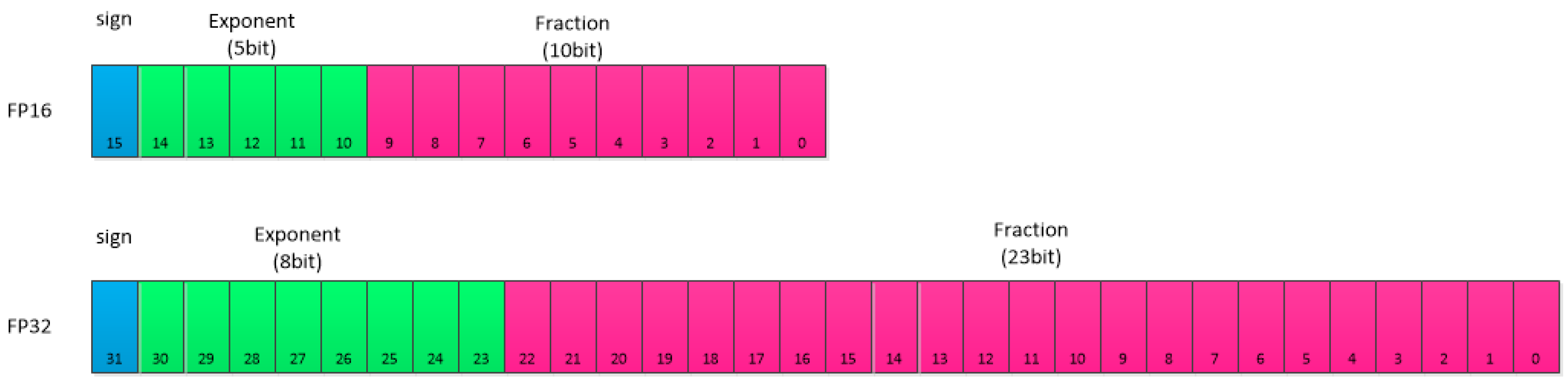
2.1. Floating-Point Data Type Parsing

In model training for deep learning, floating-point data types serve as the foundation of data representation and computation. Different floating-point data types vary in terms of storage formats and precision. According to the IEEE 754 standard [16], the value of a floating-point number is determined by the sign bit, exponent bit, and fractional bit together, Figure 1 shows the differences between FP16 and FP32, and these differences have a significant impact on the performance and results of model training. The research by Micikevicius et al. [15] shows that the storage density of FP16 is twice that of FP32, which can reduce video memory usage by 50%. However, the numerical range compression caused by low bitwidth may lead to gradient underflow. John et al. [17] systematically compared the precision loss of FP32 and FP16 for different models. Although FP16 computation is fast, FP32 has higher training accuracy.

Single-precision (FP32) floating-point numbers are encoded in 32-bit binary, where the sign bit occupies 1 bit, the exponent bit occupies 8 bits, and the fractional bit occupies 23 bits. FP32 can represent a wider range of values with higher precision and can provide more accurate results in a variety of computational tasks. In most conventional computing scenarios, such as general scientific computing, data processing, and many deep learning tasks, FP32 can fulfill the tasks well and provide an accurate numerical basis for model training and inference. However, due to its large storage bitwidth, it will take up more memory space and computational resources during model storage and computation. In some memory- and computation-sensitive scenarios, the use of FP32 faces the problem of insufficient resources, which will lead to low computational efficiency and even fail to satisfy the system’s performance requirements.

Half-precision (FP16) floating-point numbers are encoded in 16-bit binary, with 1 bit for the sign, 5 bits for the exponent, and 10 bits for the fraction. The sign bit occupies 1 bit, the exponent bit occupies 5 bits, and the fraction bit occupies 10 bits. The memory footprint of FP16 is only half the size of that of FP32, which gives FP16 an obvious advantage in storage and computation and can significantly reduce the memory footprint while lowering the computational effort. In some scenarios with limitations on computing resources, such as running deep learning models on some mobile devices or servers with limited resources, FP16 can effectively help the normal operation of the model; however, due to the small number of bits in the exponent and fractional bits, the range of values that can be represented by FP16 is narrower than that of FP32, and the accuracy is lower, which may lead to a loss of accuracy and affect the accuracy of the computation of more complex computational tasks. In more complex computational tasks, the use of FP16 may lead to a loss of accuracy and affect the performance of the model.

The differences in storage size and accuracy of different floating-point data types provide a basis for mixed-precision training. Mixed-precision training combines the advantages of different floating-point data types, so that the model can improve the training efficiency and reduce the consumption of resources under the premise of guaranteeing the accuracy, which provides more convenience in the training and application of deep learning models.

2.2. Effective Range of FP16 and FP32

For an IEEE 754-compliant floating-point number, the value V is given by

$$V={(-1)}^s\times (1+f)\times 2^{e-\mathrm{Bias}}$$

(1)

where s denotes the sign bit, occupying 1 bit, and when s = 0, it means that the floating-point number is positive; when s = 1, it means that the floating-point number is negative. e is the unsigned integer in the exponent bit, bias is the offset, which is used to express the exponent as an unsigned integer and the formula of bias (n is the number of exponential digits), and $e-Bias$ obtains the exponential value. f is the fractional part of the fractional digit representation; f is greater than or equal to 0 and less than 1. According to Equation (1), it can be calculated that the value of FP16 is in the range of −65,504 to 65,504 and is set to 0 if exceeded. FP32 has a wider range.

It can be found that the range of FP16 is much narrower than that of FP32, so the direct use of FP16 to replace FP32 will lead to the problem of top and bottom overflow in training, resulting in the loss of a large amount of data, so that the model cannot be used normally.

3. Hybrid Accuracy Training Working Mechanisms

3.1. Forward Propagation

In the forward propagation stage, the input data are usually in the FP32 format, which has high accuracy, can effectively prevent the input data from undergoing significant accuracy loss in the initial stage of the model, and can provide accurate data support for the subsequent calculation process. In operations such as convolutional computation, the data will automatically use FP16 for part of the computation according to the performance of the hardware device and the structural design of the model; on GPUs that support half-precision computation, such as NVIDIA’s Volta, Turing, and Ampere architectures, the relevant computation can be accelerated by using FP16, which can significantly increase the speed of computation. Mixed precision combines the advantages of FP32 and FP16, utilizing the high precision of FP32 to ensure the accuracy of the input data and at the same time improve the efficiency of forward propagation by taking advantage of the fast computation of FP16.

3.2. Back Propagation

Back propagation is the key process of calculating the gradient and is closely related to forward propagation. At the end of forward propagation, the model will calculate the difference between the predicted value and the true value based on the loss function. Subsequently, with the help of back propagation, the error signal is back propagated from the output layer back to the input layer, so as to calculate the gradient of each parameter. In this process, FP32 and FP16 precision are used in combination. In order to effectively reduce the amount of computation and memory consumption, the results of the intermediate calculations are generally stored and calculated using FP16.

3.3. Loss Scaling

Due to the relatively limited data representation range of FP16, underflow easily occurs when encountering very small gradient values. Once underflow occurs, the gradient information will be set to 0, thus losing the relevant data, which will seriously affect the training of the model; in order to solve this problem, we need to use gradient scaling.

Gradient scaling is one of the important processes in mixed precision training. By dynamically adjusting the scaling factor, the gradient scaling technique effectively prevents the gradient underflow problem, thus ensuring the stability of training [15]. The study shows that a reasonable choice of scaling factor can improve the training speed without the loss of accuracy. The specific work of loss scaling is to multiply the gradient values by a scaling factor in the back propagation process, so that the gradient values can be represented more accurately in the range of FP16. In the actual training, the size of the scaling factor should be adjusted according to the specific conditions of the model and the changes during the training process. If the scaling factor is too small, it may not be able to solve the problem of gradient underflow well, but if the scaling factor is too large, it may cause gradient overflow. By reasonably adjusting the scaling factor, we can ensure the accuracy of the gradient computation under FP16 precision and thus ensure normal back propagation.

3.4. Parameter Update

At the stage of updating model parameters, in order to ensure the stability of the model and the accuracy of the prediction, FP32 is used to store the parameters of the model, and the high accuracy of FP32 can effectively prevent the model performance from degradation due to the lack of accuracy in the parameter updating. After gradient scaling and back propagation, the gradient values are converted to FP32 precision, and then the parameters are updated according to the optimization algorithms used in the model, such as stochastic gradient descent, Adam, and so on.

4. Early Stopping

4.1. Fundamentals

In the reproduced paper Learning Delicate Local Representations for Multi-Person Pose Estimation [18], using the model RSN, it was found that there was an overfitting problem in the late stage of model training, so the early stopping method was introduced to optimize the model.

Early stopping has been shown to represent an effective regularization method by monitoring the validation set performance and terminating training before overfitting occurs [19]. The systematic study of the early stopping method has shown that it can significantly improve the generalization ability of the model. The core idea of early stopping is to monitor the performance of the model on the validation set during the training process. As the training progresses, the loss of the model on the training set usually decreases, and the accuracy and other indexes increase. However, after a certain point, the model’s performance on the validation set may no longer improve or even begin to decline, which means that the model may have begun to overfit; i.e., the model performs well on the training set but is less able to generalize to new and unseen data. The early stopping method means stopping training early when this trend of no improvement in the validation set performance is observed, so as to avoid overfitting the model by continuing training, and to improve the generalization ability of the model, as well as to save computational resources.

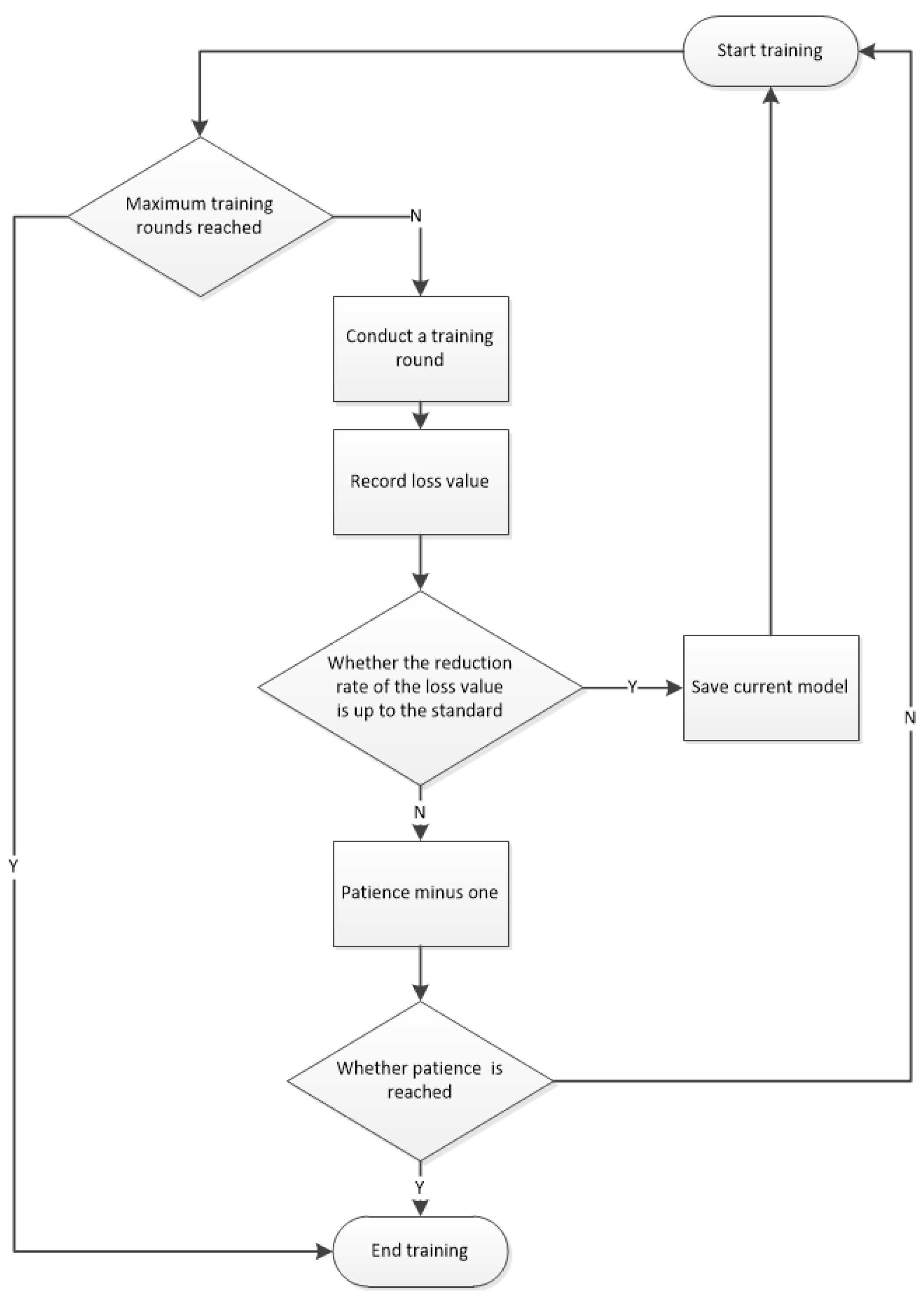
4.2. Implementation

The implementation of the early stopping method requires the selection of appropriate monitoring indicators, usually selecting the loss function value on the validation set, accuracy, etc., as the monitoring indicators, such as an image classification task to select the validation set for classification accuracy, a regression task to select the loss function value of the mean squared error, etc. We then set the stop conditions, a common way to set a fixed value for patience, such as a patience value of 10—i.e., 10 consecutive cycles of the validation set of monitoring indicators are not better than the optimal value—or we set the monitoring indicator change threshold to stop when the change is lower than the threshold; in the training process, we need to record the model when the monitoring indicators on the validation set reach the optimal value. The most common ways are to set a fixed value for patience, such as a patience value of 10—that is, 10 consecutive training cycles of the validation set monitoring indicators are not better than the previous optimal value—stop training, or set the monitoring indicator change threshold to stop when the change is lower than the threshold; in the training process, we need to record the validation set on the monitoring indicators to reach the optimal model parameters. When the stopping condition is met, the saved optimal model parameters are used as the final model parameters.The specific process is shown in Figure 2.

5. Experimentation and Analysis

5.1. Models and Datasets

The model used in this experiment is from Github [18], library name RSN. The dataset used is COCO [20]; the COCO dataset is a large and rich object detection, segmentation, and captioning dataset. This dataset is aimed at scene understanding and is mainly intercepted from complex everyday scenes, where targets in the images are localized by precise segmentation. COCO contains 80 categories and over 330,000 images, of which 200,000 are labeled, with the number of individual instances in the entire dataset exceeding 1.5 million. The COCO dataset is also labeled with 17 key points of the human body, including the head, shoulder, elbow, wrist, knee, and ankle. The labeling has high accuracy and consistency, which provides reliable supervision information for model training.

The experimental environment for this experiment was as follows. For hardware, we used the NVIDIA RTX TITAN graphics card with 24 GB high-speed video memory and with powerful parallel computing capabilities, which can efficiently deal with large-scale matrix operations in the training process of the deep learning model; CPU used the AMD R7-5700X3D processor, with 8 cores and 16 threads, a main frequency of 3 GHz, and an RWI frequency of 4.1 GHz, which can quickly respond to the computational needs of the GPU for the collaborative processing of complex computing tasks. The CPU can quickly respond to the computational needs of the GPU, and they can work together to handle complex computational tasks. There is 64 GB of DDR4 3600 MHz high-speed memory, which ensures the efficiency of data reading and writing and avoids the performance of the model being affected by insufficient memory or slow reading and writing speeds. In terms of running software, PyCharm2021 was used, compiled with python3.6, Anaconda3, pytorch1.8.1, and CUDA version 11.1.

5.2. Co-Optimization of Hybrid Accuracy and Hardware Acceleration

NVIDIA has included FP16 hardware acceleration in its architecture since the beginning of the 20-series GPUs, such as Volta, Turing, and Ampere architecture GPUs. RTX TITAN, for example, is based on the Turing architecture, and its Tensor Core supports FP16 matrix operations and FP32 accumulation (FP16-FP32), and in order to verify the hardware acceleration effect, this experiment was conducted on RTX TITAN (24 GB GDDR6 memory) with different precision statistics (FMA). In order to verify the hardware acceleration effect, this experiment was performed on the RTX TITAN (24 GB GDDR6 memory) statistics at different computational performance accuracies (see

Table 1. Computational performance at different accuracies.

Computational Operations	FP32 Calculation Time (ms)	FP16 Calculation Time (ms)	Acceleration Ratio	Tensor Core Utilization
Convolutional layer forward computation	18.6	6.2	$3.0\times$	92%
Batch normalization	2.8	1.1	$2.55\times$	35%
Gradient updates	10.3	4.5	$2.29\times$	78%

).

Table 1 shows that the Turing architecture of Tensor Core shows significant advantages in convolutional computation, and the FP16 acceleration ratio reaches 3 times, which is close to the theoretical peak. Moreover, the FP16 computation unit of RTX TITAN adopts an independent pipeline design, which can process FP32 in parallel while executing FP16 operations, thus reducing pipeline idling [21].

5.3. Dynamic Adjustment Mechanisms for Loss Scaling

In the dynamic adjustment mechanism for loss scaling, the initial scaling factor can be adjusted according to the initial distribution of the model parameters; a common setting is to set the scaling factor S to the 8th power of 2, i.e., 256, a value that can cover most of the common range of gradient values. In this paper, we adjusted S to the 7th power of 2 according to the model. After the pre-set training batch, it is necessary to check whether there is overflow; if there is overflow, then the parameter will show an NaN or Inf value. If there is no overflow, then the scaling factor is increased and S is updated to S multiplied by 2. If overflow is detected, then the scaling factor is halved and the parameter update for the current batch is skipped. Through this dynamic adjustment, the scaling factor will be stabilized between the 12th and 14th power of 2 to achieve adaptive equilibrium, thus avoiding the impact of overflow on training.

5.4. Timing of the Intervention of the Early Stopping Method

During model training, understanding the accuracy trend in the validation set is crucial in applying the early stopping method. Figure 3 shows the change in the validation set’s accuracy with the number of training epochs during the testing process, where the x-axis represents the number of training epochs and the y-axis represents the loss value.

Analyzing Figure 3, we can see that with the increase in the number of training rounds, the loss value continues to decline, showing that, in the model for the continuous learning of features in the training data, the degree of fit to the training data is growing better and better. But in the iteration of 660,000 times or so, the loss value began to stop declining significantly; there are large ups and downs, and it even has a tendency to rise repeatedly. This is the model in the training-to-late stage of the overfitting situation; we can start to intervene with the early stopping method, to avoid the model continuing to learn from the noise and details of the training data, in order to improve the model’s generalization ability. By using the early stopping method, the model’s performance can be guaranteed while avoiding wasting training time.

5.5. Comparative Experiments

The main experimental variables were the training methods, mixed-precision training, early stopping method, and early stopping method with mixed-precision training for the experimental group, and single-precision training for the control group. In order to ensure the consistency of the initial parameters of the model, the same random seed was used in all experiments when the model was initialized. The data augmentation strategies during training (random horizontal flipping, the rotation of $\pm 30$°, and scaling between 0.75 and 1.25) were independently applied across different experiments, with the data loading order in each training epoch controlled by distinct random seeds. The training set consists of 82,000 images, while the testing set contains 40,000 images. The comparison focuses on model accuracy under different IoU thresholds and training time consumption. The standard deviations reported in the table were calculated based on 4 independent experimental trials, highlighting the impact of data augmentation stochasticity and batch loading randomness on model performance.

As can be seen from

Table 2. Comparison of accuracy and time spent results for different methods.

Training Methods	AP	AP.5	AP.75	AP(M)	AP(L)	AR	Time Taken
Single precision	$0.740\pm 0.002$	$0.898\pm 0.001$	$0.810\pm 0.003$	$0.711\pm 0.004$	$0.803\pm 0.002$	$0.799\pm 0.003$	$173\mathrm{h}\pm 1\mathrm{h}$
Mixed precision	$0.738\pm 0.003$	$0.900\pm 0.002$	$0.808\pm 0.004$	$0.709\pm 0.005$	$0.801\pm 0.003$	$0.797\pm 0.004$	$132\mathrm{h}\pm 2\mathrm{h}$
Early stopping	$0.740\pm 0.002$	$0.898\pm 0.001$	$0.810\pm 0.003$	$0.711\pm 0.004$	$0.803\pm 0.001$	$0.799\pm 0.003$	$145\mathrm{h}\pm 1\mathrm{h}$
Mixed precision and early stopping	$0.738\pm 0.004$	$0.900\pm 0.003$	$0.808\pm 0.005$	$0.708\pm 0.005$	$0.801\pm 0.004$	$0.797\pm 0.005$	$113\mathrm{h}\pm 2\mathrm{h}$

, the single-precision training takes the longest time; the mixed-precision training time decreases by about 40 h with an almost negligible loss of accuracy, and even the average accuracy under the specific IoU threshold AP.5 is slightly higher than that of the single-precision training. After using the early stopping method, the training time decreases by about 28 h without any loss of accuracy; finally, the combination of mixed-precision training and the early stopping method results in a decrease of about 60 h, with a negligible loss of accuracy compared with that of the single-precision training. Finally, by combining the mixed accuracy training with the early stopping method, the training time was decreased by about 60 h compared with the single accuracy training, and the loss of accuracy was also negligible.

In summary, using the hybrid accuracy method with early stopping can significantly reduce the model training time while maintaining the accuracy and is suitable for use on resource-constrained devices.

6. Conclusions

Human pose estimation has a broad range of application prospects in the field of computer vision, but the training of the model requires a large amount of computational resources and the training time is also long. In this paper, we mainly discuss the optimization ability of the mixed-precision training and early stopping method in the training process of a human pose estimation model, analyze the floating-point data type in depth, introduce forward propagation, back propagation, loss scaling and parameter updating in detail, explain the working mechanism of mixed-precision training from various angles, and introduce the principle and implementation of the early stopping method at the same time. The experimental results show that the introduction of mixed-precision training into the human posture estimation model can significantly improve the training speed, and there is almost no loss of accuracy, and the average accuracy of mixed-precision training is even slightly higher than that of single-precision training when the IoU threshold is AP.5; the use of early stopping method not only prevents the model from overfitting but also significantly reduces the training time. The best result is achieved by the combination of the mixed-precision training and the early stopping method, compared with the single-precision training, which is the most effective. The combination of mixed-precision training and the early stopping method has the best effect, and, compared with single-precision training, the training time is reduced by about 60 h, while the accuracy remains stable.

This study contributes greatly to the development of human pose estimation, especially providing a new solution for model training in resource-constrained environments; using mixed-accuracy training, researchers can train and study human pose estimation models more quickly and efficiently, which strongly promotes the practical application of human pose estimation techniques in more scenarios. However, the acceleration effect of mixed-precision training highly depends on the hardware’s native support for FP16. For example, NVIDIA GPUs based on the Volta, Turing, and Ampere architectures can accelerate FP16 matrix operations, but non-NVIDIA GPUs or older hardware lacking dedicated FP16 computing units will have limited acceleration effects. Meanwhile, in scenarios involving ultra-large-scale models, high complexity in distributed training, or extreme sensitivity to precision, it is necessary to verify through experiments whether the precision loss is acceptable and integrate other technical optimizations.

References

- Cao, Z.; Simon, T.; Wei, S.E.; Sheikh, Y. Realtime Multi-Person 2D Pose Estimation using Part Affinity Fields. In Proceedings of the IEEE Conference on Computer Vision and Pattern Recognition, Honolulu, HI, USA, 21–26 July 2017; pp. 7291–7300. [Google Scholar]
- Toshev, A.; Szegedy, C. DeepPose: Human Pose Estimation via Deep Neural Networks. In Proceedings of the IEEE Conference on Computer Vision and Pattern Recognition (CVPR), Columbus, OH, USA, 24–27 June 2014; pp. 1653–1660. [Google Scholar]
- Pavllo, D.; Feichtenhofer, C.; Grangier, D.; Auli, M. 3D Human Pose Estimation in Video with Temporal Convolutions and Semi-Supervised Training. In Proceedings of the IEEE/CVF Conference on Computer Vision and Pattern Recognition (CVPR), Long Beach, CA, USA, 15–20 June 2019; pp. 7334–7343. [Google Scholar]
- Fang, H.S.; Li, J.F.; Tang, H.Y.; Xu, C.; Zhu, H.; Xiu, Y.; Li, Y.L.; Lu, C. AlphaPose: Whole-Body Regional Multi-Person Pose Estimation and Tracking in Real-Time. IEEE Trans. Pattern Anal. Mach. Intell. (TPAMI) 2022, 45, 7157–7173. [Google Scholar] [CrossRef] [PubMed]
- Clever, H.M.; Erickson, Z.; Kapusta, A.; Turk, G.; Liu, C.K.; Kemp, C.C. Bodies at Rest: 3D Human Pose and Shape Estimation from a Pressure Image using Synthetic Data. In Proceedings of the IEEE/CVF Conference on Computer Vision and Pattern Recognition (CVPR), Seattle, WA, USA, 14–19 June 2020; pp. 6215–6224. [Google Scholar]
- Zheng, C.; Zhu, S.; Mendieta, M.; Yang, T.; Chen, C.; Ding, Z. 3D Human Pose Estimation with Spatial and Temporal Transformers. In Proceedings of the IEEE/CVF International Conference on Computer Vision, Montreal, QC, Canada, 11–17 October 2021; pp. 11656–11665. [Google Scholar]
- Mehraban, S.; Taatit, B.; Adeli, V. MotionAgformer: Enhancing 3D Human Pose Estimation with a Transformer-GCN Formernetwork. In Proceedings of the IEEE/CVF Winter Conference on Applications of Computer Vision, Waikoloa, HI, USA, 3–8 January 2024. [Google Scholar]
- Pinheiro, G.S.; Jin, X.; Da Costa, V.T.; Lames, M. Body pose estimation integrated with notational analysis: A new approach to analyze penalty kicks strategy in elite football. Front. Sports Act. Living 2022, 4, 818556. [Google Scholar] [CrossRef] [PubMed]
- Tan, M.X.; Le, Q.V. EfficientNet: Rethinking Model Scaling for Convolutional Neural Networks. In Proceedings of the International Conference on Machine Learning (ICML), Long Beach, CA, USA, 9–15 June 2019. [Google Scholar]
- Yuan, Y.H.; Fu, R.; Huang, L.; Lin, W.; Zhang, C.; Chen, X.; Wang, J. HRFormer: High-Resolution Transformer for Dense Prediction. In Proceedings of the Conference on Neural Information Processing Systems (NeurIPS), Online, 6–14 December 2021. [Google Scholar]
- Rajbhandari, S.; Rasley, J.; Ruwase, O.; He, Y. ZeRO: Memory Optimizations Toward Training Trillion Parameter Models. In Proceedings of the International Conference for High Performance Computing, Networking, Storage and Analysis (SC20), Online, 9–19 November 2020; pp. 379–388. [Google Scholar]
- Xu, J.; Zhou, W.; Fu, Z.; Zhou, H.; Li, L. A Survey on Green Deep Learning. arXiv 2021, arXiv:2111.05193. [Google Scholar]
- Liu, Y.; Hua, J. L-HRNet: A Lightweight High-Resolution Network for Human Pose Estimation. In Proceedings of the 2023 8th International Conference on Intelligent Informatics and Biomedical Sciences (ICIIBMS), Okinawa, Japan, 23–25 November 2023. [Google Scholar]
- Hou, B.; Chen, Q.; Wang, J.; Yin, G.; Wang, C.; Du, N.; Pang, R.; Chang, S.; Lei, T. Instruction-Following Pruning for Large Language Models. arXiv 2025, arXiv:2501.02086. [Google Scholar]
- Micikevicius, P.; Narang, S.; Alben, J.; Diamos, G.; Elsen, E.; Garcia, D.; Ginsburg, B.; Houston, M.; Kuchaiev, O.; Venkatesh, G.; et al. Mixed Precision Training. arXiv 2017, arXiv:1710.03740. [Google Scholar]
- IEEE 754-2008; IEEE Standard for Floating-Point Arithmetic. IEEE: Piscataway, NJ, USA, 2008.
- Ríos, J.O.; Armejach, A.; Petit, E.; Henry, G.; Casas, M. Dynamically Adapting Floating-Point Precision to Accelerate Deep Neural Network Training. In Proceedings of the 2021 IEEE International Conference on Machine Learning and Applications (ICMLA), Virtual, 13–16 December 2021. [Google Scholar]
- Cai, Y.; Wang, Z.; Luo, Z.X.; Yin, B.; Du, A.; Wang, H.; Zhang, X.; Zhou, X.; Zhou, E.; Sun, J. Learning Delicate Local Representations for Multi-Person Pose Estimation. In Proceedings of the European Conference on Computer Vision (ECCV), Glasgow, UK, 23–28 August 2020. [Google Scholar]
- Prechelt, L. Early Stopping—But When? Springer: Berlin/Heidelberg, Germany, 1998; pp. 55–69. [Google Scholar]
- Lin, T.Y.; Maire, M.; Belongie, S.; Hays, J.; Perona, P.; Ramanan, D.; Dollár, P.; Zitnick, C.L. Microsoft COCO: Common Objects in Context. In Proceedings of the European Conference on Computer Vision (ECCV); Springer: Berlin/Heidelberg, Germany, 2014; pp. 740–755. [Google Scholar]
- NVIDIA Corporation. Turing Architecture Whitepaper(R). 2018. Available online: https://www.nvidia.cn/geforce/news/geforce-rtx-20-series-turing-architecture-whitepaper (accessed on 11 June 2025).