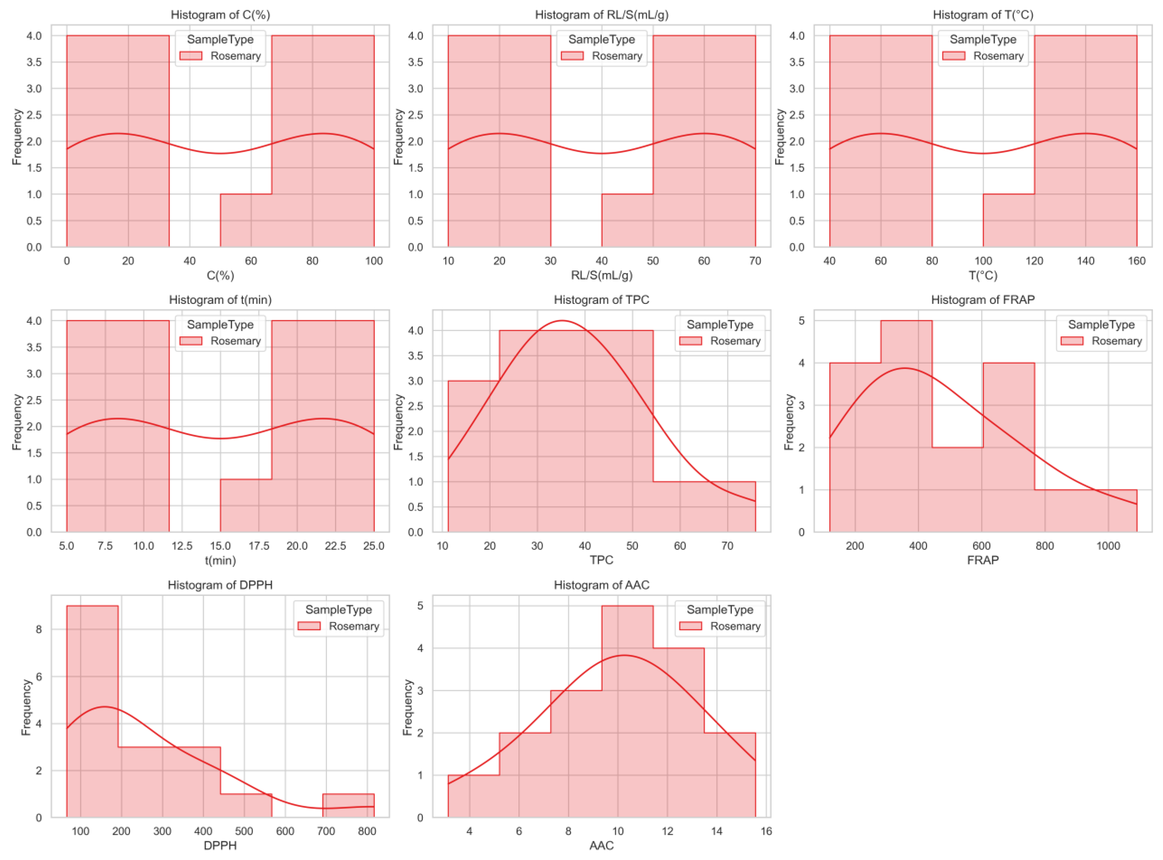
Figure 1.
Histograms with kernel density estimates showing the distribution of extraction parameters and antioxidant response variables for rosemary samples. While extraction settings are uniformly distributed due to the design structure, antioxidant responses such as FRAP and DPPH exhibit skewed distributions, indicating variability in sample performance.
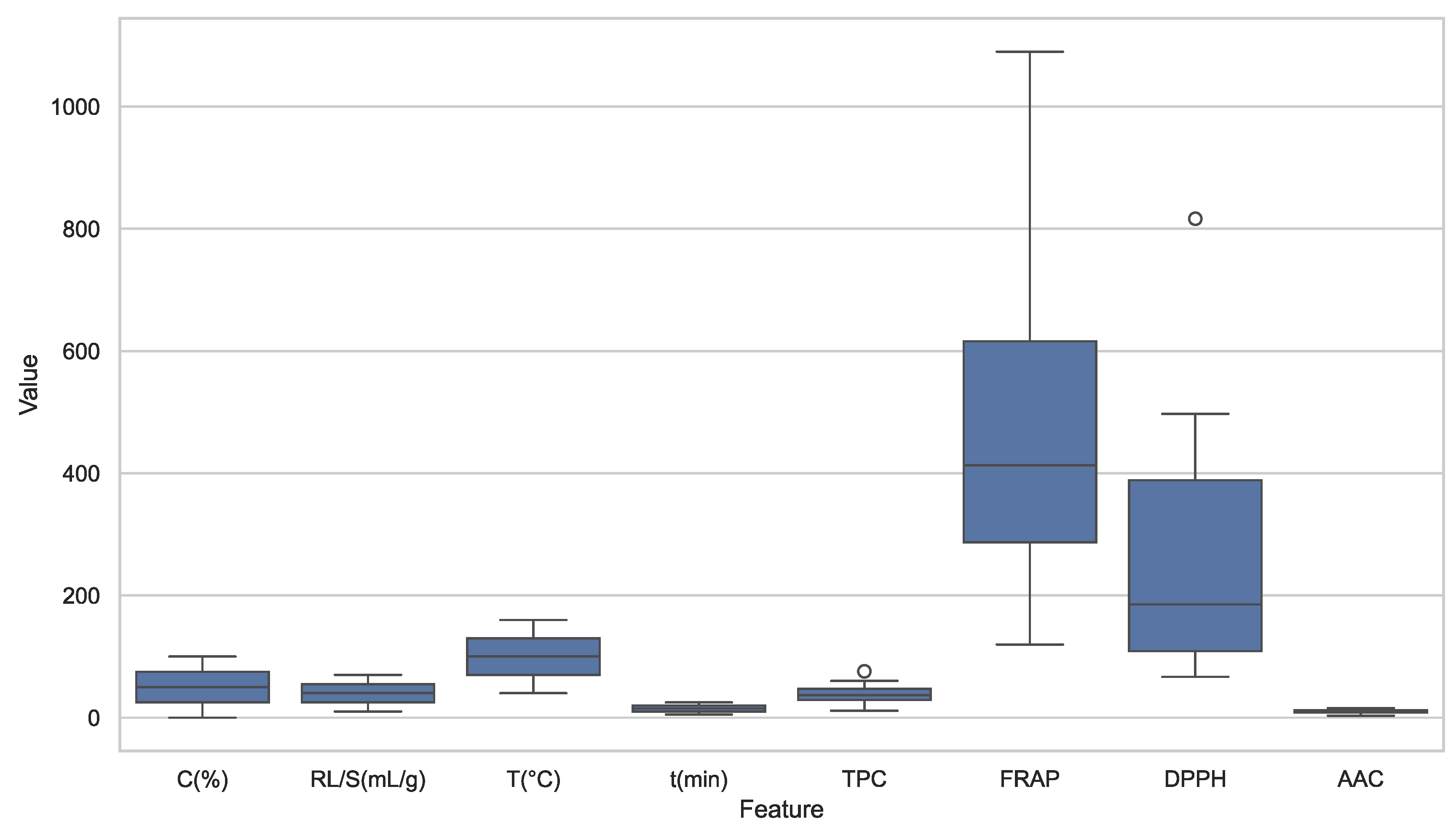
Figure 2.
Combined boxplot of all extraction parameters and antioxidant response variables. Antioxidant metrics (FRAP and DPPH) exhibit larger spread and more outliers than extraction parameters, indicating greater variability and sensitivity to experimental conditions.
Figure 2.
Combined boxplot of all extraction parameters and antioxidant response variables. Antioxidant metrics (FRAP and DPPH) exhibit larger spread and more outliers than extraction parameters, indicating greater variability and sensitivity to experimental conditions.
Figure 3.
Plot (A) is a heatmap of raw data values for extraction parameters and antioxidant responses across 17 experimental conditions. Brighter colors indicate higher absolute values. The most intense FRAP activity was observed in sample #13. Plot (B) is a z-score normalized heatmap of the same dataset. Standardization enables direct comparison across all features. Red shades represent values above the mean, while blue shades indicate values below the mean. Strong positive deviations in FRAP and TPC are evident in sample #13.
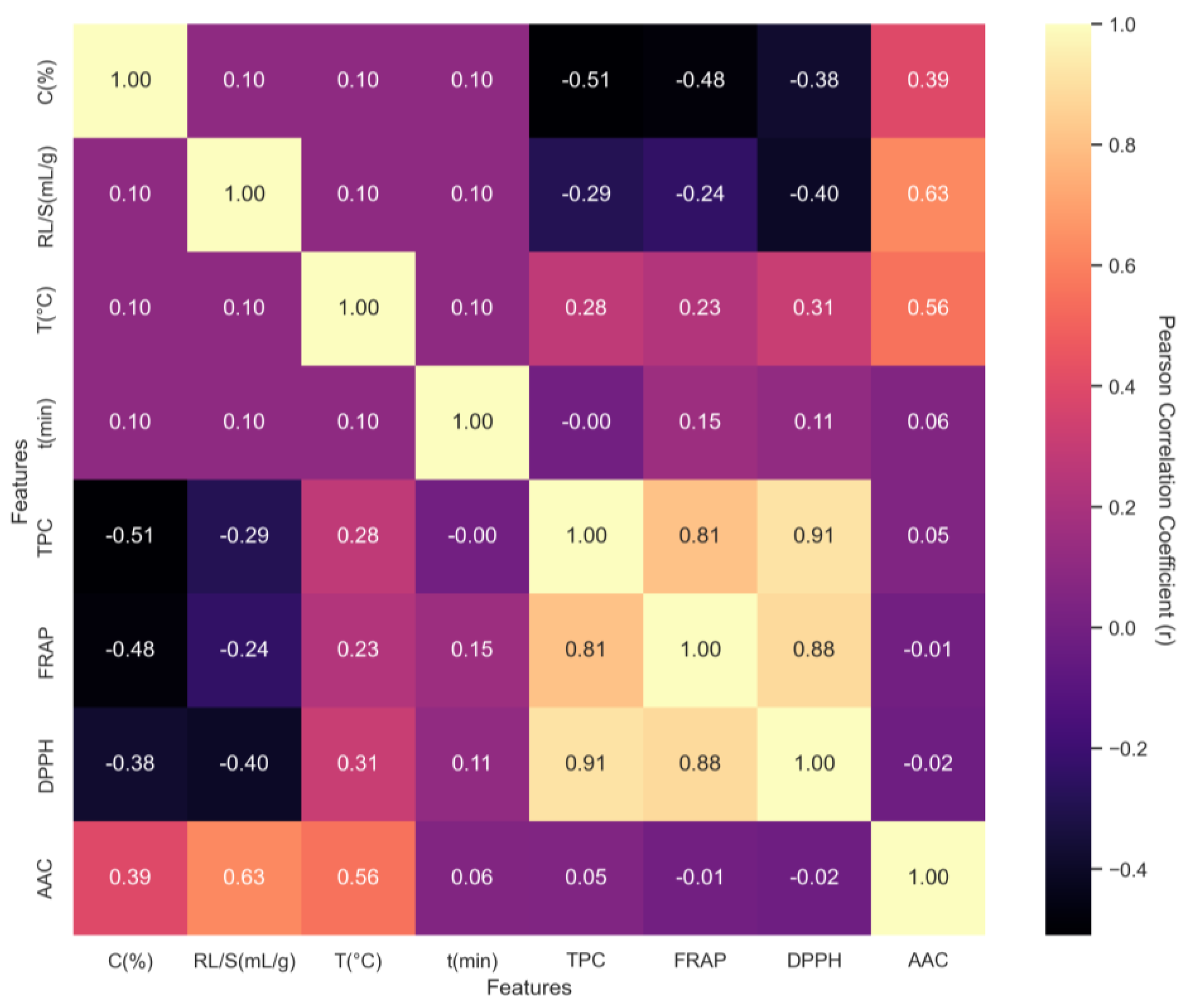
Figure 4.
Pearson correlation matrix among extraction parameters and antioxidant response variables. Values range from −1 (perfect negative correlation) to +1 (perfect positive correlation). Strong internal consistency was observed among antioxidant metrics (TPC, FRAP, and DPPH), while concentration (C, %) negatively correlates with TPC and FRAP.
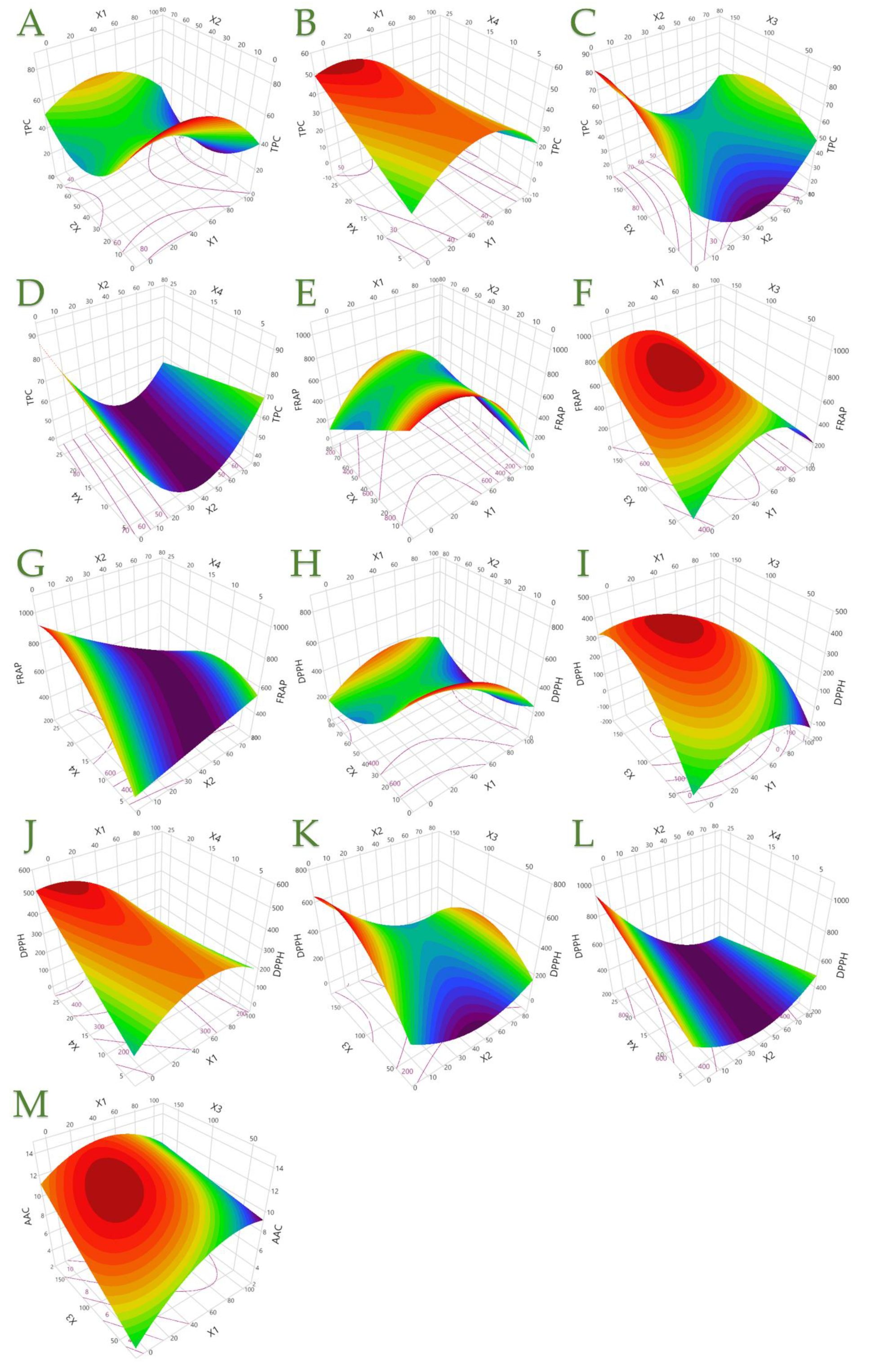
Figure 5.
TPC, showing the (A) covariation of X1 (ethanol concentration, C, % v/v) and X2 (liquid-to-solid ratio, R, mL/g); (B) covariation of X1 and X4 (extraction time, t, min); (C) covariation of X2 and X3 (extraction temperature, T, °C); and (D) covariation of X2 and X4. FRAP, showing the (E) covariation of X1 and X2; (F) covariation of X1 and X3; and (G) covariation of X2 and X4. DPPH, showing the (H) covariation of X1 and X2; (I) covariation of X1 and X3; (J) covariation of X1 and X4; (K) covariation of X2 and X3; and (L) covariation of X2 and X4. AAC, showing the (M) covariation of X1 and X3.
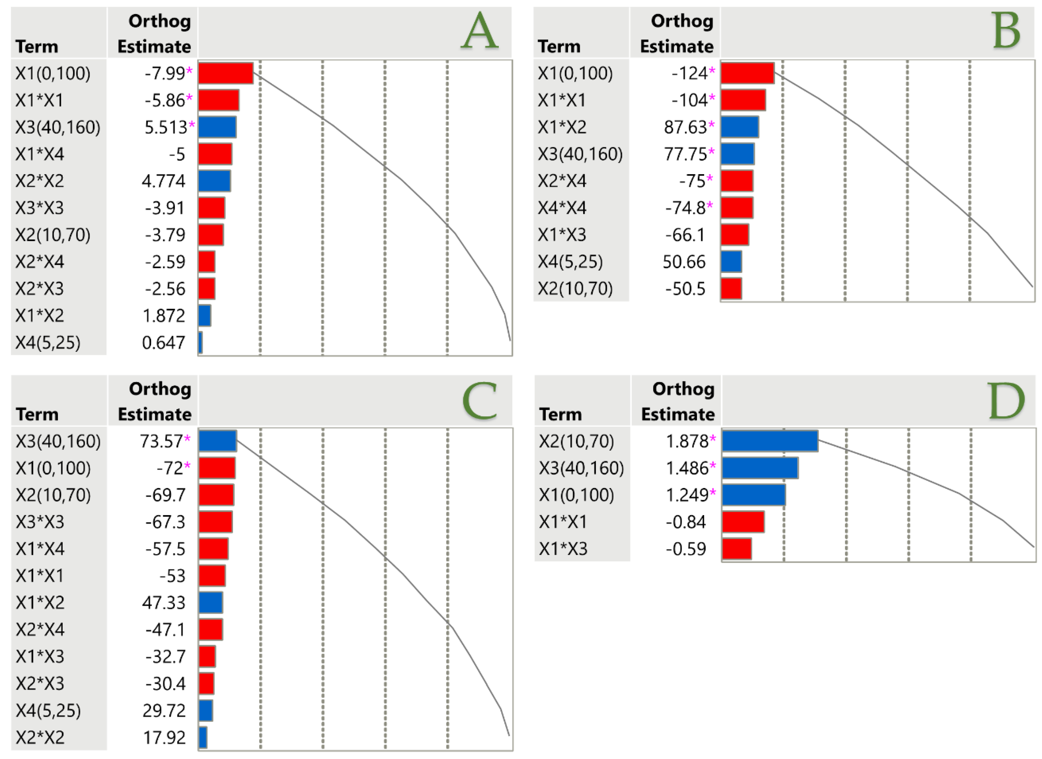
Figure 6.
Pareto plots illustrating the significance of parameter estimates for the PLE technique across TPC (A), FRAP (B), DPPH (C), and AAC (D), with a pink asterisk marking significant values (p < 0.05). Positive estimates are shown in blue, while negative ones are represented in red.
Figure 6.
Pareto plots illustrating the significance of parameter estimates for the PLE technique across TPC (A), FRAP (B), DPPH (C), and AAC (D), with a pink asterisk marking significant values (p < 0.05). Positive estimates are shown in blue, while negative ones are represented in red.
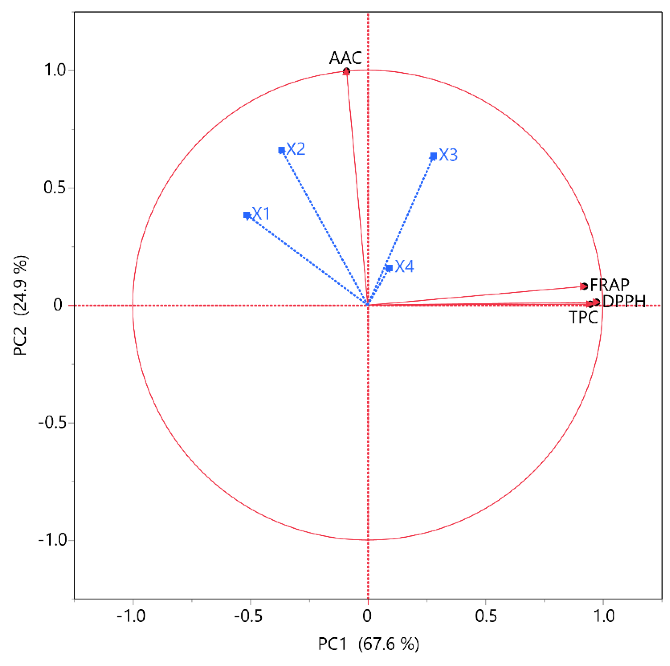
Figure 7.
PCA for the measured variables. Each X variable is presented with a blue color.
Figure 7.
PCA for the measured variables. Each X variable is presented with a blue color.
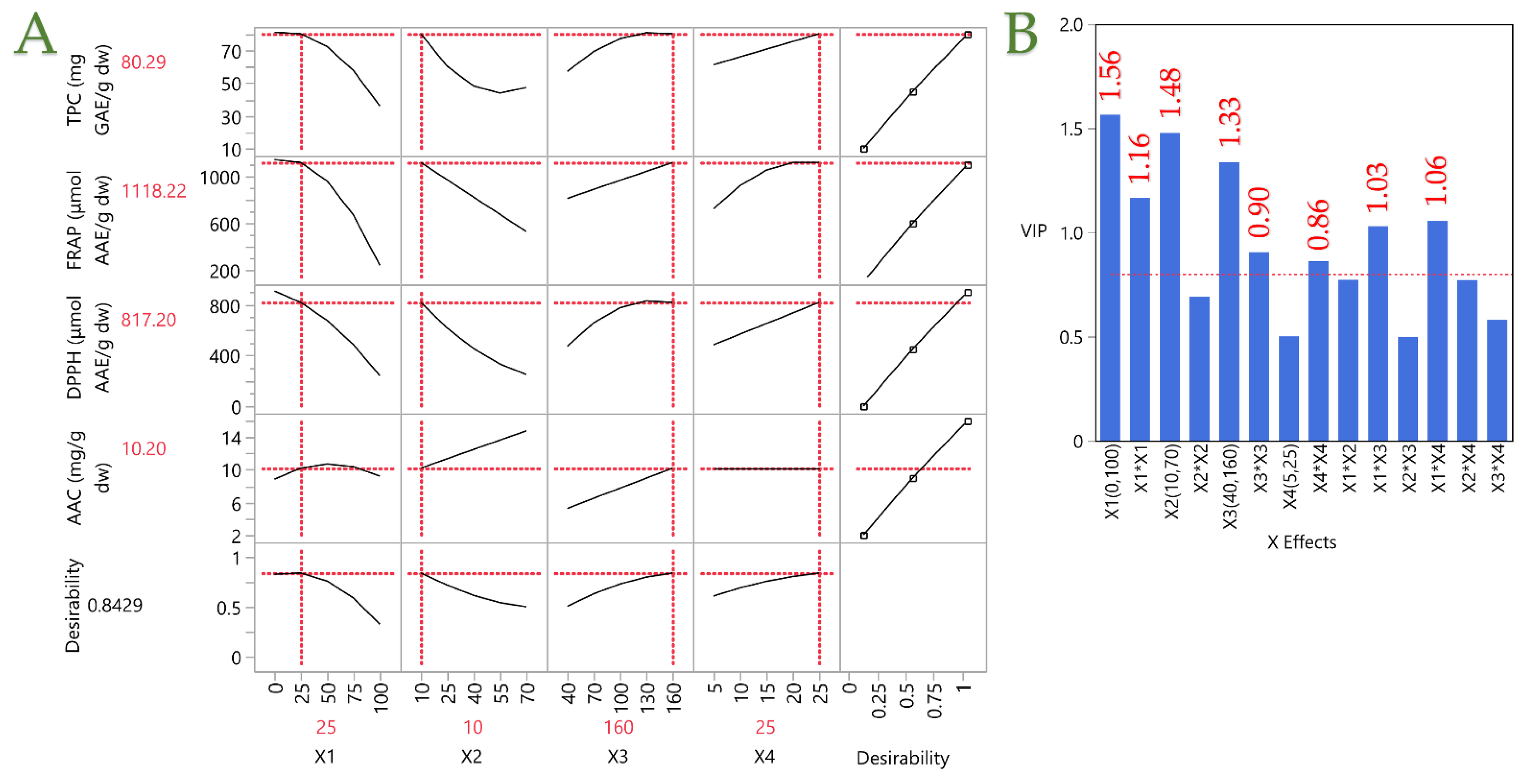
Figure 8.
Plot (A) shows the optimization of the PLE technique for rosemary extracts through the partial least squares (PLS) prediction profiler and a desirability function with extrapolation control. Plot (B) shows the Variable Importance Plot (VIP) graph, showing the VIP values for each predictor variable in the PLE technique, with a red dashed line marking the 0.8 significance level.
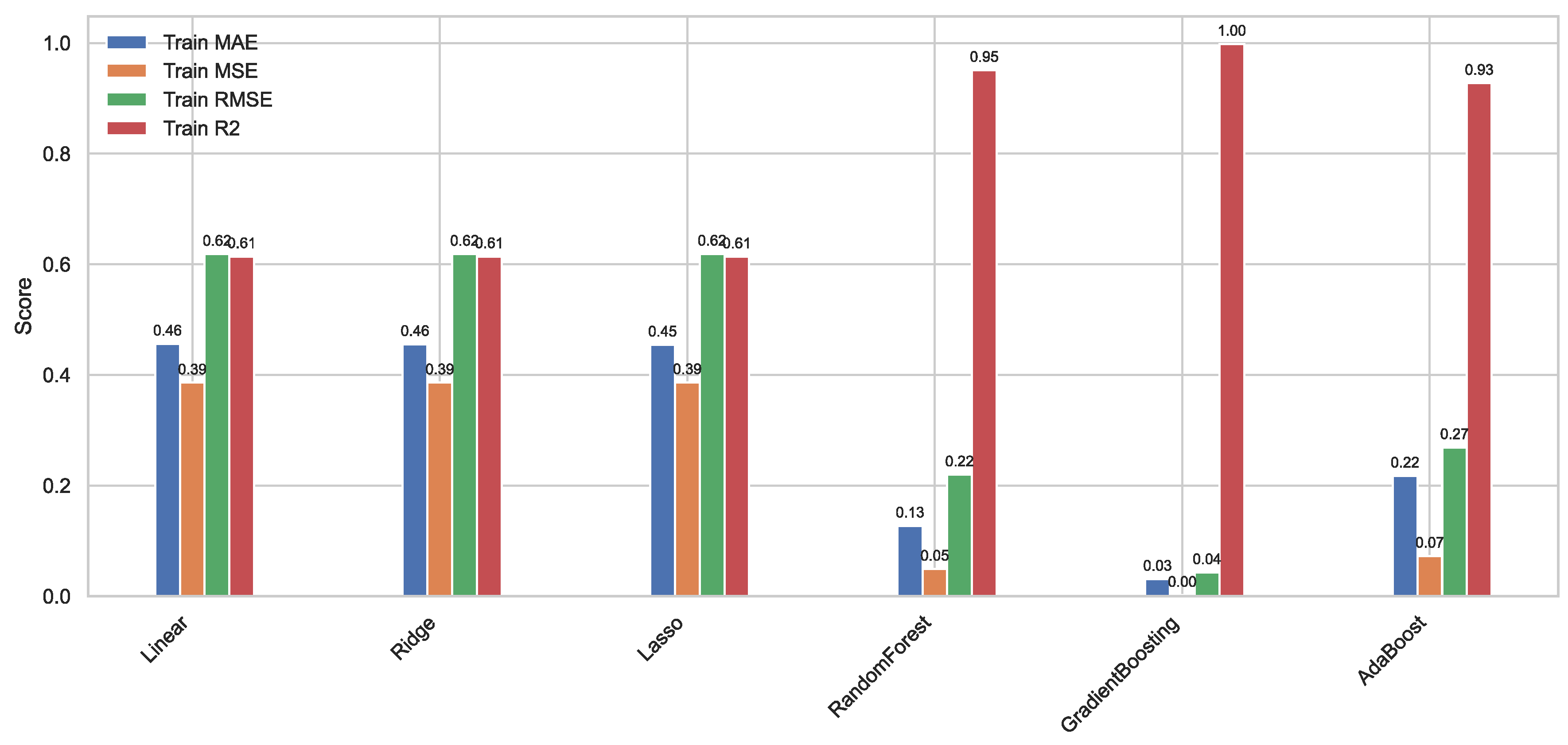
Figure 9.
Histograms of the performance of our six ML models on our original training set.
Figure 9.
Histograms of the performance of our six ML models on our original training set.
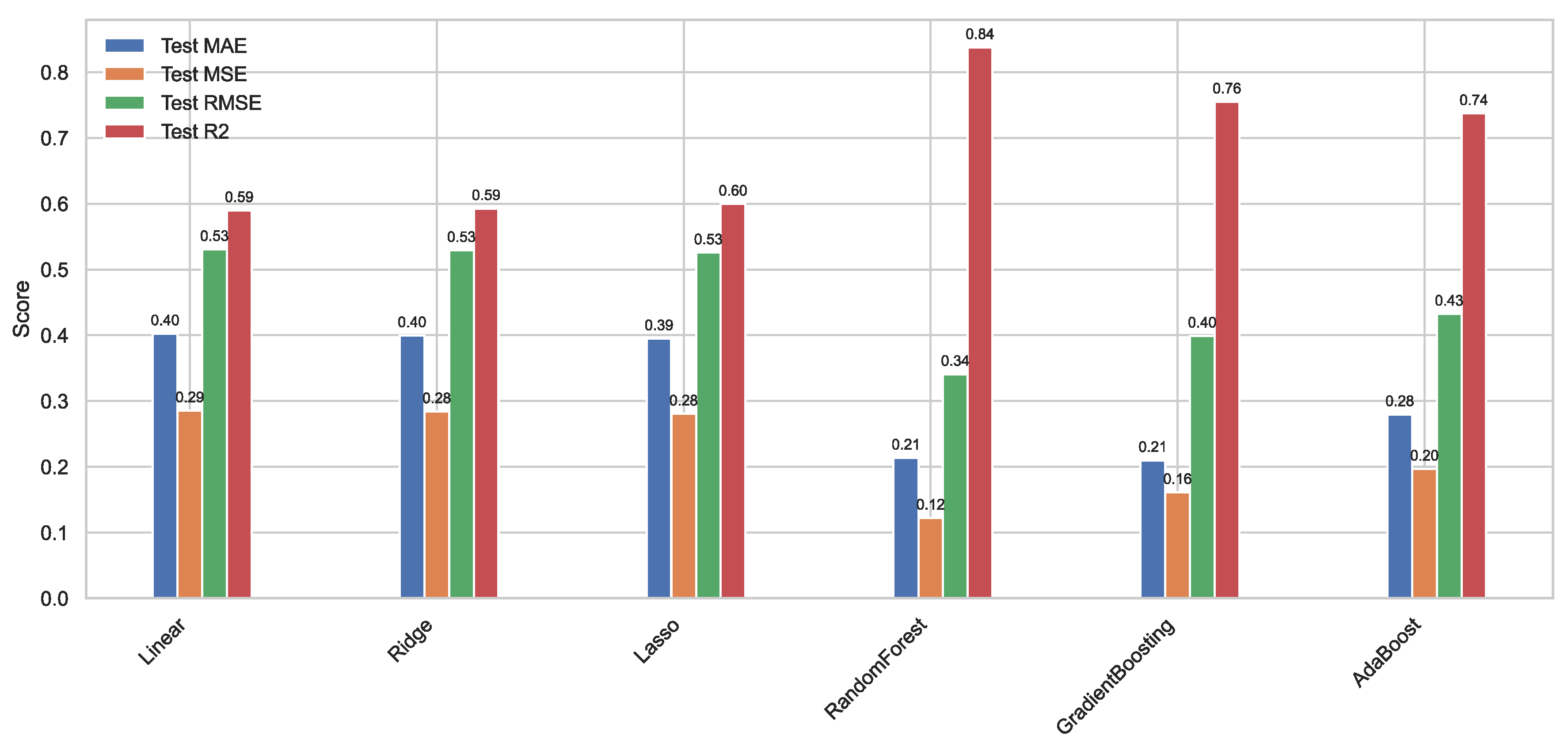
Figure 10.
Histograms of the performance of our six ML models on our original test set.
Figure 10.
Histograms of the performance of our six ML models on our original test set.
Figure 11.
Histograms of the performance of our six ML models on our synthetic training set.
Figure 11.
Histograms of the performance of our six ML models on our synthetic training set.
Figure 12.
Histograms of the performance of our six ML models on our synthetic test set.
Figure 12.
Histograms of the performance of our six ML models on our synthetic test set.
Figure 13.
Histograms of the performance of our six ML models on our mixed training set.
Figure 13.
Histograms of the performance of our six ML models on our mixed training set.
Figure 14.
Histograms of the performance of our six ML models on our mixed test set.
Figure 14.
Histograms of the performance of our six ML models on our mixed test set.
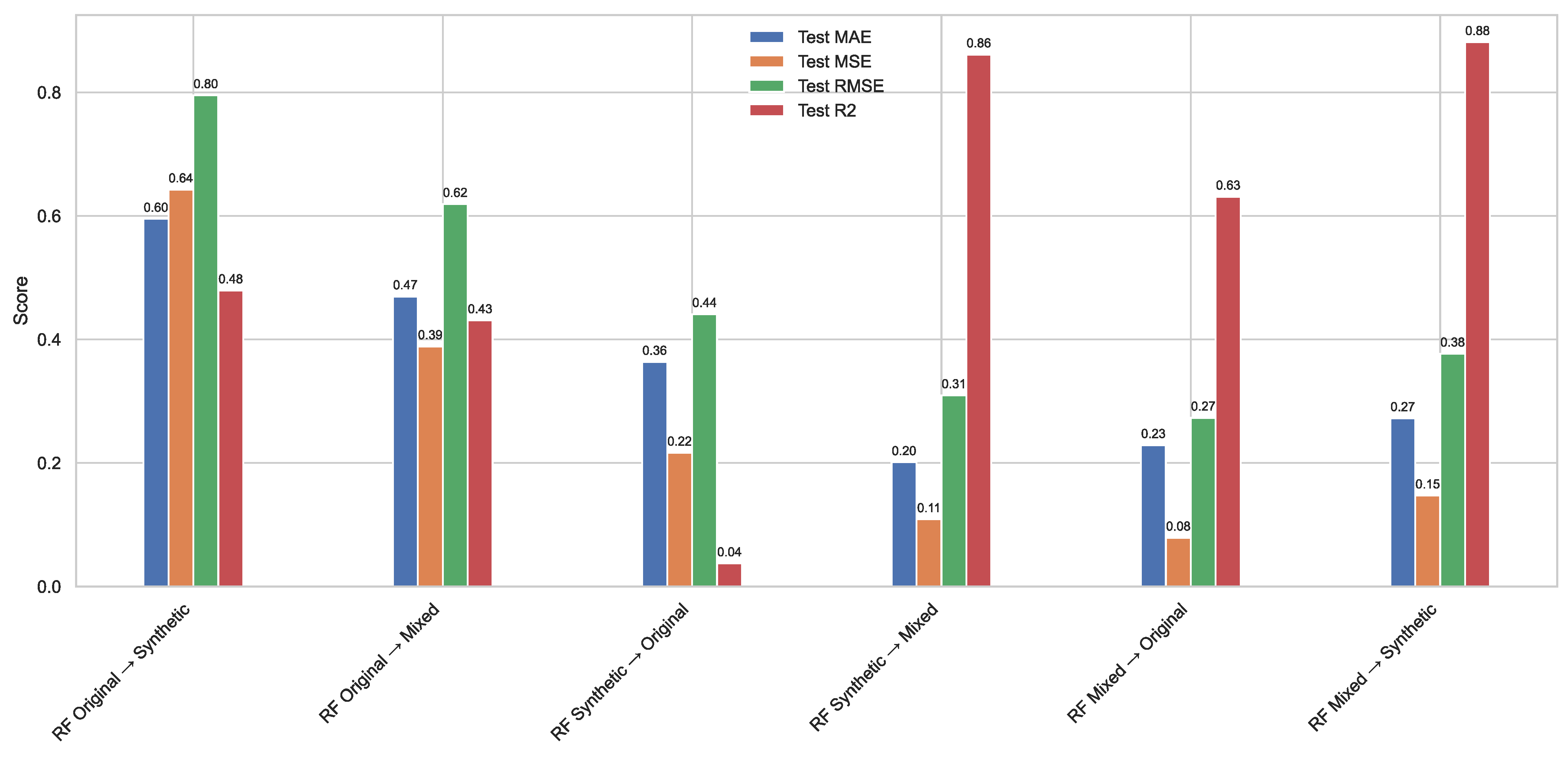
Figure 15.
Cross-dataset evaluation of the RF regression model trained on the original, synthetic, and mixed datasets. Each group of bars represents the performance metrics MAE, MSE, RMSE, and R2 obtained when the model trained on one dataset was tested on another. Results highlight the generalization ability of each training regime across data domains. Models trained on the mixed dataset showed superior cross-domain performance, particularly when evaluated on both the original and synthetic test sets.
Figure 16.
Feature importance scores from RF models trained on the (left) original, (middle) synthetic, and (right) mixed datasets. Importance scores reflect each feature’s contribution to predicting antioxidant targets (TPC, FRAP, DPPH, and AAC). Feature influence varies significantly depending on the dataset used for training.
Figure 17.
Predicted vs. actual standardized values for antioxidant targets using RF-based models trained on the original (top row), synthetic (middle row), and mixed (bottom row) datasets. Diagonal red dashed lines represent the ideal 1:1 relationship. R2 values quantify model fit for each case.
Figure 17.
Predicted vs. actual standardized values for antioxidant targets using RF-based models trained on the original (top row), synthetic (middle row), and mixed (bottom row) datasets. Diagonal red dashed lines represent the ideal 1:1 relationship. R2 values quantify model fit for each case.
Figure 18.
Partial dependence plots showing the marginal effect of each feature on antioxidant predictions from the RF original model.
Figure 18.
Partial dependence plots showing the marginal effect of each feature on antioxidant predictions from the RF original model.
Figure 19.
Partial dependence plots showing the marginal effect of each feature on antioxidant predictions from the RF synthetic model.
Figure 19.
Partial dependence plots showing the marginal effect of each feature on antioxidant predictions from the RF synthetic model.
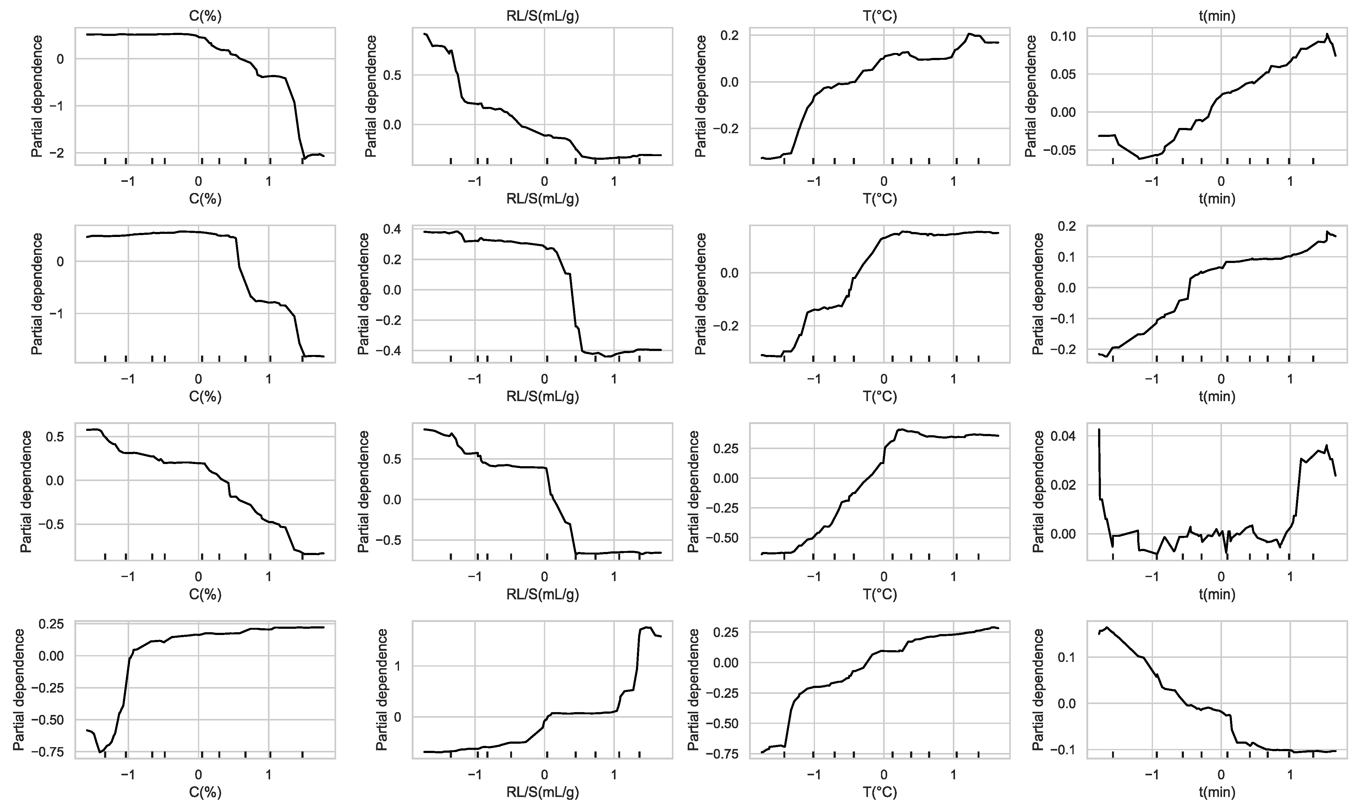
Figure 20.
Partial dependence plots showing the marginal effect of each feature on antioxidant predictions from the RF mixed model.
Figure 20.
Partial dependence plots showing the marginal effect of each feature on antioxidant predictions from the RF mixed model.
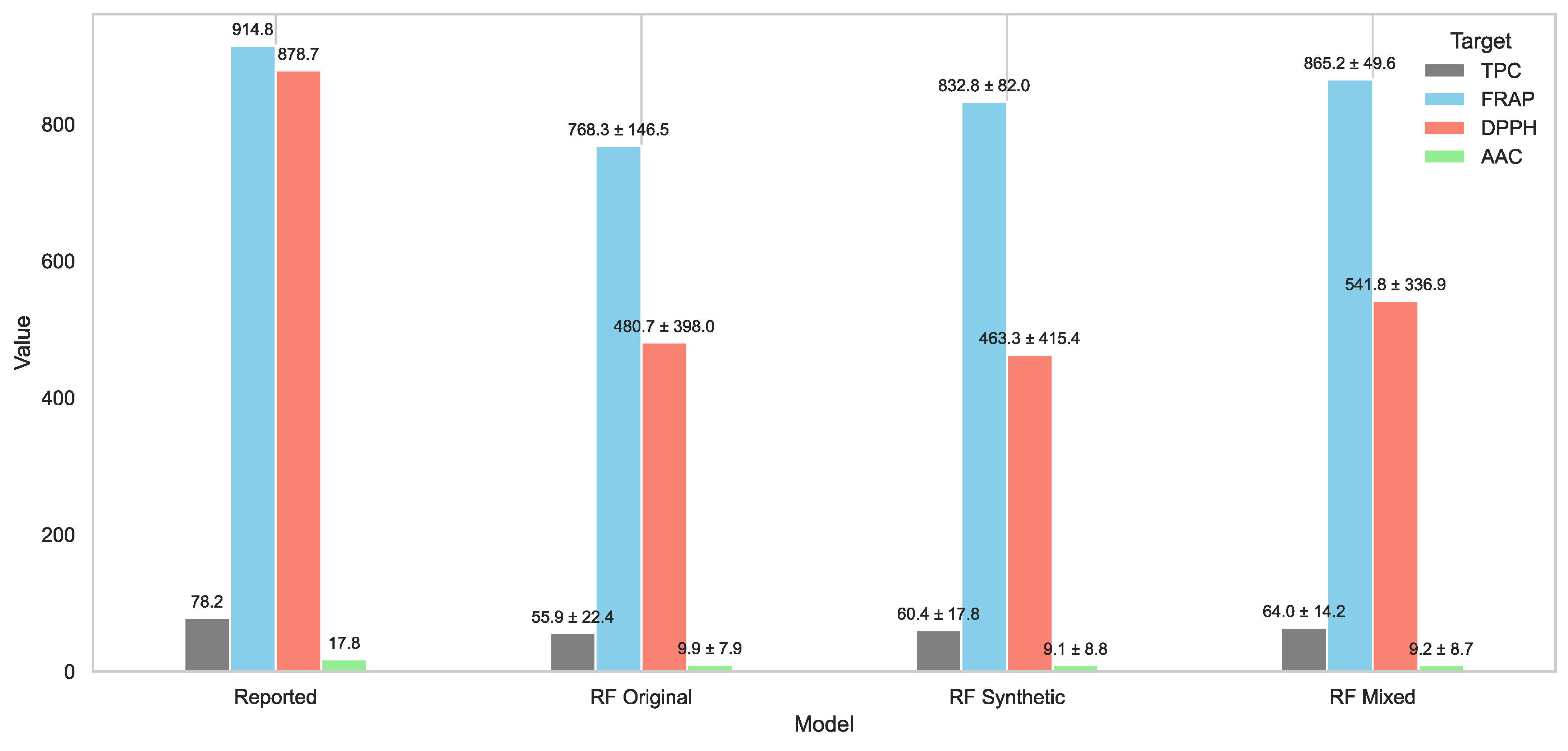
Figure 21.
Comparison of predicted versus reported antioxidant values under optimal extraction conditions using RF-based models trained on the original, synthetic, and mixed datasets. Bars represent predicted values for TPC, FRAP, DPPH, and AAC, with numeric labels showing predicted value ± absolute error relative to the experimentally reported values. The mixed model produced the most accurate predictions overall, with reduced errors across most targets.
Table 1.
Summary of machine learning regression models and the corresponding hyperparameters tuned during grid search. Default parameters were used for Linear Regression, while regularization strengths (α) and core structural parameters (number of estimators, max depth, min samples split, tree depth, and learning rate) were varied for the other models.
| Model | Tuned Parameters | Values Tested |
|---|
| Linear Regression | None | - |
| Ridge | α | [0.1, 1.0, 10.0] |
| Lasso | α | [0.001, 0.01, 0.1, 1.0] |
| RF | n_estimators, max_depth, min_samples_split | [100, 200], [None, 10], [2, 5] |
| GB | n_estimators, learning_rate, max_depth | [100, 200], [0.05, 0.1], [3, 5] |
| AdaBoost | n_estimators, learning_rate | [50, 100], [0.5, 1.0] |
Table 2.
Experimental results for the four examined independent variables and the dependent variables’ responses to the PLE technique.
Table 2.
Experimental results for the four examined independent variables and the dependent variables’ responses to the PLE technique.
| Design Point | Independent Variables | Actual PLE Responses * |
|---|
| C (%) (X1) | RL/S (mL/g) (X2) | T (°C) (X3) | t (min) (X4) | TPC | FRAP | DPPH | AAC |
|---|
| 1 | 75 | 10 | 40 | 20 | 37.20 | 612.74 | 243.81 | 7.47 |
| 2 | 75 | 55 | 130 | 20 | 26.84 | 366.39 | 152.88 | 9.46 |
| 3 | 25 | 25 | 160 | 10 | 44.43 | 740.02 | 389.29 | 9.95 |
| 4 | 0 | 55 | 130 | 5 | 37.03 | 451.66 | 230.22 | 12.02 |
| 5 | 0 | 10 | 40 | 5 | 28.84 | 331.68 | 67.14 | 3.14 |
| 6 | 100 | 25 | 160 | 25 | 18.96 | 214.42 | 108.73 | 9.90 |
| 7 | 100 | 70 | 160 | 10 | 34.14 | 413.30 | 174.82 | 14.65 |
| 8 | 100 | 25 | 70 | 10 | 11.26 | 119.68 | 66.67 | 8.35 |
| 9 | 25 | 70 | 70 | 10 | 41.10 | 467.27 | 185.26 | 11.05 |
| 10 | 25 | 70 | 160 | 25 | 47.41 | 615.91 | 251.75 | 15.56 |
| 11 | 75 | 10 | 130 | 5 | 60.26 | 286.87 | 388.69 | 11.89 |
| 12 | 0 | 55 | 40 | 20 | 31.88 | 233.39 | 100.86 | 5.45 |
| 13 | 0 | 10 | 130 | 20 | 75.85 | 1089.81 | 816.36 | 6.38 |
| 14 | 75 | 55 | 40 | 5 | 30.09 | 393.47 | 150.16 | 10.24 |
| 15 | 100 | 70 | 70 | 25 | 19.17 | 169.93 | 85.11 | 13.34 |
| 16 | 25 | 25 | 70 | 25 | 49.64 | 696.79 | 427.46 | 8.44 |
| 17 | 50 | 40 | 100 | 15 | 52.69 | 893.17 | 497.11 | 12.45 |
Table 3.
Analysis of variance (ANOVA) is performed for the response surface quadratic polynomial model in the context of the PLE technique.
Table 3.
Analysis of variance (ANOVA) is performed for the response surface quadratic polynomial model in the context of the PLE technique.
| Factor | TPC | FRAP | DPPH | AAC |
|---|
| Stepwise regression coefficients | | | | |
| Intercept | 42.88 * | 715.8 * | 356.2 * | 11.04 * |
| X1—ethanol concentration | −10.7 * | −170 * | −96.8 * | 1.204 * |
| X2—liquid-to-solid ratio | −5.69 | −81.1 | −103 * | 2.283 * |
| X3—temperature | 7.183 | 96.73 * | 93.54 * | 1.956 * |
| X4—extraction time | 0.854 | 66.9 | 39.24 | - |
| X1X2 | 3.746 | 166.6 * | 92.01 | - |
| X1X3 | - | −114 | −54.1 | −1.02 |
| X1X4 | −8.19 | - | −91 | - |
| X2X3 | −4.4 | - | −52.1 | - |
| X2X4 | −4.51 | −131 * | −82.1 | - |
| X3X4 | - | - | - | - |
| X12 | −13.8 | −268 * | −103 | −1.69 |
| X22 | 15.5 | - | 79.73 | - |
| X32 | −8.56 | - | −130 | - |
| X42 | - | −131 | - | - |
| ANOVA | | | | |
| F-value | 4.507 | 7.716 | 4.362 | 10.65 |
| p-Value | 0.0545 ns | 0.0067 * | 0.0833 ns | 0.0006 * |
| R2 | 0.908 | 0.908 | 0.929 | 0.829 |
| Adjusted R2 | 0.707 | 0.791 | 0.716 | 0.751 |
| RMSE | 8.747 | 121.9 | 104.7 | 1.633 |
| PRESS | 3913 | 363,375 | 580,653 | 57.61 |
| CV | 42.46 | 55.93 | 77.03 | 32.76 |
| DF (total) | 16 | 16 | 16 | 16 |
Table 4.
Maximum predicted responses and optimum extraction conditions for the dependent variables.
Table 4.
Maximum predicted responses and optimum extraction conditions for the dependent variables.
| Parameters | Independent Variables | Desirability | Stepwise Regression |
|---|
| C (%) (X1) | RL/S (mL/g) (X2) | T (°C) (X3) | t (min) (X4) |
|---|
| TPC (mg GAE/g dw) | 25 | 10 | 130 | 20 | 0.9292 | 76.19 ± 17.92 |
| FRAP (μmol AAE/g dw) | 25 | 10 | 160 | 20 | 0.9907 | 1117.68 ± 212.88 |
| DPPH (μmol AAE/g dw) | 0 | 10 | 130 | 20 | 0.8728 | 799.03 ± 271.68 |
| AAC (mg/g dw) | 50 | 70 | 160 | - | 0.9318 | 15.28 ± 2.23 |
Table 5.
Multivariate correlation analysis of measured variables.
Table 5.
Multivariate correlation analysis of measured variables.
| Responses | TPC | FRAP | DPPH | AAC |
|---|
| TPC | – | 0.7796 | 0.9129 | −0.0738 |
| FRAP | | – | 0.8549 | −0.0139 |
| DPPH | | | – | −0.0722 |
| AAC | | | | – |
Table 6.
The partial least squares (PLS) prediction profiler determined the maximum desirability for all variables under optimal extraction condition for PLE technique.
Table 6.
The partial least squares (PLS) prediction profiler determined the maximum desirability for all variables under optimal extraction condition for PLE technique.
| Parameters | Independent Variables | Desirability | Partial Least Squares (PLS) Regression | Experimental Values |
|---|
| C (%) (X1) | RL/S (mL/g) (X2) | T (°C) (X3) | t (min) (X4) |
|---|
| TPC (mg GAE/g dw) | 25 | 10 | 160 | 25 | 0.8429 | 80.29 | 78.23 ± 0.63 |
| FRAP (μmol AAE/g dw) | 1118.22 | 914.82 ± 1.53 |
| DPPH (μmol AAE/g dw) | 817.20 | 878.7 ± 6.34 |
| AAC (mg/g dw) | 10.20 | 17.83 ± 0.25 |
Table 7.
Optimal extraction conditions for polyphenolic compounds using the PLE technique of rosemary extraction.
Table 7.
Optimal extraction conditions for polyphenolic compounds using the PLE technique of rosemary extraction.
| Polyphenolic Compound | Concentration (μg/g dw) |
|---|
| Catechin | 239 ± 11 |
| Quercetin 3-D-galactoside | 1114 ± 45 |
| Luteolin-7-glucoside | 236 ± 13 |
| Kaempferol-3-glucoside | 442 ± 19 |
| Hesperidin | 3711 ± 96 |
| Rosmarinic acid | 1570 ± 58 |
| Apigenin | 245 ± 7 |
| Kaempferol | 72 ± 2 |
| Rosmanol | 731 ± 27 |
| Carnosic acid | 889 ± 32 |
| Total identified | 9250 ± 311 |
Table 8.
Equation of calibration curves for each compound identified through HPLC-DAD.
Table 8.
Equation of calibration curves for each compound identified through HPLC-DAD.
| Polyphenolic Compounds (Standards) | Equation (Linear) | R2 | Retention Time (min) | UVmax (nm) |
|---|
| Catechin | y = 11,920.78x − 128.19 | 0.997 | 20.933 | 278 |
| Quercetin 3-D-galactoside | y = 41,489.69x − 35,577.55 | 0.993 | 34.598 | 257 |
| Luteolin-7-glucoside | y = 34,875.94x − 16,827.36 | 0.999 | 35.949 | 347 |
| Kaempferol-3-glucoside | y = 50,916.85x − 42,398.83 | 0.996 | 38.724 | 265 |
| Hesperidin | y = −30,502.75x − 30,502.75 | 0.995 | 40.249 | 283 |
| Rosmarinic acid | y = 50,281.27x − 113,633.31 | 0.995 | 41.644 | 329 |
| Apigenin | y = 95,483.52x − 5214.26 | 0.998 | 55.860 | 227 |
| Kaempferol | y = 93,385.02x − 18,613.03 | 0.999 | 56.883 | 265 |
| Rosmanol | y = 5509.45x − 10,899.23 | 0.994 | 65.924 | 288 |
| Carnosic acid | y = 8883.45x + 101,483.30 | 0.992 | 77.870 | 284 |


 ,
, 


