Dimension-Adaptive Machine Learning for Efficient Uncertainty Quantification in Geological Carbon Storage Models

Abstract

Carbon capture and storage (CCS) plays a role in mitigating climate change, but effective implementation requires accurate prediction of CO₂ behavior in geological formations. This study introduces a novel machine learning framework for quantifying uncertainty across 2D and 3D carbon storage models. We develop a dimension-adaptive Bayesian neural network architecture that enables efficient knowledge transfer between dimensional representations while maintaining physical consistency. The framework incorporates aleatoric uncertainty from inherent geological variability and epistemic uncertainty from model limitations. Trained on over 5000 high-fidelity simulations across multiple geological scenarios, our approach demonstrates superior computational efficiency, reducing analysis time for 3D models by 87% while maintaining prediction accuracy within 5% of full simulations. The framework effectively captures complex uncertainty patterns in spatiotemporal CO₂ plume evolution. It identifies previously unrecognized parameter interdependencies, particularly between vertical permeability anisotropy and capillary entry pressure, which significantly impact plume migration in 3D models but are often overlooked in 2D representations. Compared with traditional Monte Carlo methods, our approach provides more accurate uncertainty bounds and enhanced identification of high-risk scenarios. This multidimensional framework enables rapid assessment of storage capacity and leakage risk under uncertainty, providing a practical tool for CCS site selection and operational decision-making across dimensional scales.

1. Introduction

Carbon capture and storage (CCS) represents a critical technology for reducing greenhouse gas emissions and mitigating climate change impacts [1,2]. The Intergovernmental Panel on Climate Change (IPCC) has identified CCS as an essential component of pathways limiting global warming to 1.5 °C above pre-industrial levels [1]. While our study focuses on the storage component, it is important to acknowledge that effective CCS implementation requires the integration of capture technologies with secure storage solutions [3]. Successful implementation of CCS requires safe and efficient storage of CO₂ in suitable geological formations, typically deep saline aquifers or depleted hydrocarbon reservoirs [4]. However, significant uncertainties exist regarding subsurface CO₂ migration, trapping mechanisms, and potential leakage pathways [5,6]. Numerical modeling of subsurface CO₂ storage provides crucial insights for site selection, capacity estimation, and risk assessment [7].

Traditionally, such modeling has employed either two-dimensional (2D) or three-dimensional (3D) approaches, each with distinct advantages and limitations. Two-dimensional models offer computational efficiency and simplified representation, making them suitable for rapid screening and uncertainty analysis [8]. In contrast, three-dimensional models provide a more realistic representation of complex geological structures and flow dynamics, but at significantly higher computational cost [9,10]. This dimensional dichotomy presents a fundamental challenge in carbon storage modeling: balancing computational tractability with physical representativeness across dimensional scales.

Uncertainty quantification (UQ) is essential for the reliable prediction of CO₂ behavior in geological formations [11]. Sources of uncertainty in carbon storage models include heterogeneous reservoir properties, fluid-rock interactions, and boundary conditions [12]. Traditional UQ approaches, such as Monte Carlo simulation, require numerous model evaluations, which become prohibitively expensive for 3D models [13,14]. This computational bottleneck has limited comprehensive uncertainty assessment in carbon storage projects, potentially leading to inadequate risk evaluation [15].

Recent advances in machine learning (ML) offer promising solutions for efficient surrogate modeling and uncertainty quantification in geoscience applications [16,17]. Deep neural networks, Gaussian processes, and ensemble methods have demonstrated success in emulating complex physical systems while substantially reducing computational demands [18]. The evolution of neural network techniques has significantly impacted interpretability [19] and enhanced performance in complex process systems through various architectural approaches [20]. However, most existing ML approaches for carbon storage modeling are dimension-specific, failing to leverage the complementary information available across 2D and 3D representations [21,22]. Additionally, existing methods often inadequately quantify predictive uncertainty, focusing primarily on point predictions rather than comprehensive uncertainty bounds [23].

The limitations of current approaches highlight a significant research gap, that is, the need for dimension-adaptive uncertainty quantification methods that can efficiently transfer knowledge between 2D and 3D carbon storage models while providing a comprehensive uncertainty assessment. Addressing this gap would enable more robust decision-making in CCS projects while minimizing computational requirements.

This paper introduces a novel machine learning framework for uncertainty quantification across dimensional scales in carbon storage modeling. Our key contributions include the development of a dimension-adaptive Bayesian neural network architecture capable of processing both 2D and 3D spatial data while maintaining physical consistency; the implementation of cross-dimensional transfer learning techniques that leverage information from computationally efficient 2D models to enhance predictions in 3D domains; comprehensive uncertainty quantification approach that distinguishes between aleatoric uncertainty (inherent variability) and epistemic uncertainty (model limitations) across dimensional scales; demonstration of significant computational efficiency gains while maintaining high prediction accuracy in both 2D and 3D scenarios; and identification of critical parameters driving uncertainty in carbon storage predictions and their dimensional dependence. These advances directly address critical needs in carbon storage implementation by enabling rapid multi-scenario risk assessment during site selection; optimizing injection strategies through real-time uncertainty quantification; guiding monitoring system design through targeted uncertainty mapping; and supporting regulatory compliance by quantifying prediction confidence intervals across dimensional representations. By bridging the gap between computational efficiency and physical representativeness, our framework provides practical tools for accelerating carbon storage deployment at commercial scales.

The remainder of this paper is organized as follows: Section 2 reviews background literature on carbon storage modeling, uncertainty quantification, and relevant machine learning approaches. Section 3 details our methodology, including the 2D and 3D model formulations, dataset generation, and the dimension-adaptive machine learning architecture. Section 4 presents results demonstrating performance, uncertainty quantification capabilities, and computational efficiency of our approach. Section 5 discusses the implications of our findings, limitations, and real-world applicability. Finally, Section 6 summarizes our conclusions and suggests directions for future research.

2. Background and Related Work

2.1. Carbon Storage Modeling Approaches Across Dimensional Scales

Numerical modeling of carbon storage in geological formations has evolved significantly over the past decades. Two-dimensional modeling approaches have been widely employed for their computational efficiency and ability to capture essential physical processes. Early 2D models focused on vertical cross-sections to investigate gravity-driven flow and capillary trapping [24]. Subsequent work expanded these approaches with benchmark 2D problems incorporating heterogeneity and multiple phases [25]. More recently, the effectiveness of vertically integrated 2D models for the rapid assessment of large-scale CO₂ migration patterns has been demonstrated [26]. Three-dimensional modeling approaches provide more realistic representations of complex geological structures, but at a substantially higher computational cost. Comprehensive 3D models incorporating detailed geological characterization predict CO₂ plume evolution in heterogeneous formations [27]. Other 3D models incorporate coupled geomechanical effects to assess caprock integrity during CO₂ injection [28,29]. The importance of 3D representation for accurately capturing gravity override and heterogeneity effects on plume migration has also been highlighted [29]. The relationship between 2D and 3D modeling approaches has been explored through dimensional reduction techniques, such as vertical equilibrium models that approximate 3D physics using 2D computational domains [30]. Comparisons between dimensionally reduced models and full 3D simulations identify scenarios where simplified models adequately capture essential behavior [31]. These efforts highlight the potential for cross-dimensional knowledge transfer but have not fully leveraged modern machine learning techniques for efficient dimensional upscaling.

2.2. Sources of Uncertainty in 2D Versus 3D Carbon Storage Models

Uncertainty in carbon storage modeling stems from multiple sources with varying significance across dimensional representations. In both 2D and 3D models, petrophysical properties such as permeability and porosity represent primary uncertainty sources [32]. Spatial heterogeneity in these properties significantly impacts CO₂ migration patterns [33]. However, the representation of heterogeneity differs substantially between dimensions, with 3D models capturing spatial correlation structures more completely than 2D approximations [34]. Structural uncertainties exhibit strong dimensional dependence. While 2D models can represent major structural features like faults and formation dip, they inadequately capture complex 3D geometries and connectivity [35]. Structural representation in 3D models critically affects trapping mechanism quantification [36]. Additionally, 3D models better capture boundary condition uncertainties related to regional flow patterns and interaction with surrounding formations [37]. Process uncertainties also vary across dimensional scales. Two-dimensional models often rely on simplified representations of complex processes such as gravity segregation, capillary trapping, and dissolution [38]. These simplifications introduce systematic uncertainties compared to full 3D physics [38]. Furthermore, dimensional representation affects uncertainty in coupled processes, with 3D models better capturing thermal, geomechanical, and geochemical interactions [39]. The propagation of these uncertainties through models of different dimensionality remains insufficiently understood. Traditional approaches analyze uncertainty separately in each dimensional context without leveraging cross-dimensional relationships [40]. This gap highlights the need for uncertainty quantification methods that can systematically compare and transfer uncertainty characterization across dimensional scales.

2.3. Machine Learning for Cross-Dimensional Surrogate Modeling

Machine learning approaches have emerged as powerful tools for creating surrogate models that emulate complex physical simulations at reduced computational cost. Deep learning models have been implemented for carbon storage applications to predict CO₂ plume evolution in 2D domains and capture multiphase flow dynamics in heterogeneous porous media [16,41,42]. Physics-informed neural networks incorporate domain knowledge to improve prediction accuracy while ensuring physical consistency [43]. Dimension-specific architectures address the unique characteristics of different spatial representations. For 2D modeling, U-Net architectures prove effective for capturing spatial patterns [44]. For 3D applications, 3D CNNs and graph neural networks show promise in capturing complex spatial relationships [45]. However, most existing approaches treat dimensional representations as separate domains, failing to leverage complementary information. Recent advances in transfer learning offer promising directions for cross-dimensional knowledge transfer. Pre-training on simplified models can improve performance on complex simulations [46]. Domain adaptation techniques transfer knowledge between related subsurface flow problems [47]. Multi-fidelity modeling approaches combine high-fidelity (3D) and low-fidelity (2D) simulations to improve accuracy while reducing computational requirements [48]. Despite these advances, machine learning for carbon storage modeling faces challenges. Most methods focus on deterministic predictions rather than comprehensive uncertainty quantification [49]. Additionally, preserving physical constraints across dimensional transformations remains challenging [50]. These limitations highlight the need for dimension-adaptive machine learning approaches that maintain physical consistency while providing robust uncertainty quantification. As shown in

Table 1. Comparison of our dimension-adaptive ML framework with existing ML-UQ approaches for CCS.

Feature	This Work	Zhu & Zabaras [18]	3D CNNs [45]	Dropout-Based UQ [51]
Dimensional capability	2D and 3D with cross-dimensional transfer	Single dimension (2D)	Single dimension (3D)	Single dimension (2D)
UQ approach	Bayesian neural networks with aleatoric and epistemic uncertainty separation	Bayesian deep convolutional encoder-decoder	Deterministic with ensemble-based UQ	Monte Carlo dropout
Physical constraints	Explicit physics-informed constraints	Implicit through data	None	None
Parameter interdependencies	Explicitly modeled	Not addressed	Not addressed	Not addressed
Computational efficiency	104–105 × vs. Monte Carlo	103 × vs. Monte Carlo	103 × vs. Monte Carlo	102 × vs. Monte Carlo
Real-world applicability	Tested on multiple geological scenarios	Limited to synthetic cases	Single reservoir type	Single reservoir type

, our dimension-adaptive machine learning framework demonstrates superior capabilities across multiple features compared to existing approaches, including dimensional flexibility, uncertainty quantification methodology, and computational efficiency.

2.4. Uncertainty Quantification Techniques for Dimensional Transfer

Uncertainty quantification in surrogate modeling has advanced with probabilistic machine learning methods. Bayesian neural networks provide a framework for estimating predictive uncertainty in deep learning [52]. Deep ensembles offer a non-Bayesian alternative for uncertainty estimation [53,54]. These approaches enable the distinction between aleatoric uncertainty (inherent data variability) and epistemic uncertainty (model limitations) [55,56]. For geoscience applications, Gaussian process regression quantifies uncertainty in subsurface flow [57]. Dropout-based Bayesian approximation in CNNs quantifies uncertainty in CO₂ plume predictions [51]. These methods predominantly focus on single-dimensional applications, without addressing uncertainties introduced during dimensional transfer. The challenges of UQ across dimensional scales have received limited attention. Analysis shows uncertainty propagates differently in vertically integrated models compared to full 3D simulations [58]. Calibration techniques can correct for biases introduced by dimensional reduction [59]. However, comprehensive frameworks for quantifying and transferring uncertainty across dimensions remain underdeveloped. Multi-fidelity uncertainty quantification offers relevant insights. Approaches combine low-fidelity (e.g., 2D) and high-fidelity (e.g., 3D) models to improve prediction accuracy with quantified uncertainty [60,61]. Foundational methods calibrate simplified models using limited high-fidelity data [62]. Adapting these approaches to dimensional transfer challenges in carbon storage modeling could significantly advance UQ capabilities while maintaining computational efficiency. The literature reveals opportunities for advancing carbon storage modeling through dimension-adaptive ML. By combining advances in transfer learning, UQ, and physics-informed networks, more efficient and accurate methods for predicting CO₂ behavior across dimensions can be developed.

3. Materials and Methods

3.1. Mathematical Formulation of Carbon Storage Models

3.1.1. 2D Carbon Storage Model

Our two-dimensional model represents a vertical cross-section of a saline aquifer with CO₂ injection. The model incorporates the two-phase flow (CO₂ and brine) in porous media governed by mass conservation principles and Darcy’s law. For the CO₂ phase, the mass conservation equation is expressed as follows [63]:

$${\displaystyle \frac{\partial }{\partial t}}\left(\varphi {\rho }_c{S}_c\right)+\nabla ·\left({\rho }_c{\mathbf{u}}_c\right)=q_c$$

(1)

where $\varphi$ is porosity, ${\rho }_c$ is CO₂ density, $S_c$ is CO₂ saturation, ${\mathbf{u}}_c$ is the Darcy velocity of CO₂, and $q_c$ is the source/sink term. Similarly, for the brine phase:

$${\displaystyle \frac{\partial }{\partial t}}\left(\varphi {\rho }_b{S}_b\right)+\nabla ·\left({\rho }_b{\mathbf{u}}_b\right)=q_b$$

(2)

where subscript b denotes brine properties. The phase saturations sum to unity:

$$S_c+S_b=1$$

(3)

The Darcy velocities for each phase are determined by the following:

$${\mathbf{u}}_c=-{\displaystyle \frac{k_{r,c}}{{\mu }_c}}\mathbf{K}·(\nabla p_c-{\rho }_{c}g\nabla z)$$

(4)

$${\mathbf{u}}_b=-{\displaystyle \frac{k_{r,b}}{{\mu }_b}}\mathbf{K}·(\nabla p_b-{\rho }_{b}g\nabla z)$$

(5)

where $k_{r,c}$ and $k_{r,b}$ are relative permeabilities, ${\mu }_c$ and ${\mu }_b$ are dynamic viscosities, $\mathbf{K}$ is the absolute permeability tensor, $p_c$ and $p_b$ are phase pressures, g is gravitational acceleration, and z is the vertical coordinate. The phase pressures are related through the capillary pressure:

$$p_c-p_b=p_{cap}\left(S_b\right)$$

(6)

For the 2D model, we employ the Brooks–Corey relation [64] for relative permeability and capillary pressure:

$$k_{r,c}=k_{r,c}^0{\left({\displaystyle \frac{1-S_b-S_{r,c}}{1-S_{r,b}-S_{r,c}}}\right)}^{n_c}$$

(7)

$$k_{r,b}=k_{r,b}^0{\left({\displaystyle \frac{S_b-S_{r,b}}{1-S_{r,b}-S_{r,c}}}\right)}^{n_b}$$

(8)

$$p_{cap}=p_e{\left({\displaystyle \frac{S_b-S_{r,b}}{1-S_{r,b}-S_{r,c}}}\right)}^{-1/\lambda }$$

(9)

where $S_{r,c}$ and $S_{r,b}$ are residual saturations, $k_{r,c}^0$ and $k_{r,b}^0$ are endpoint relative permeabilities, $n_c$ and $n_b$ are exponents, $p_e$ is entry pressure, and $\lambda$ is the pore size distribution index. The 2D model domain represents a vertical cross-section with dimensions of 5 km × 0.1 km, discretized into a 500 × 50 grid. The domain incorporates heterogeneous permeability and porosity fields generated using sequential Gaussian simulation with specified correlation lengths and variance [65]. We consider five geological layers with contrasting properties, representing alternating aquitards and aquifers. The CO₂ injection occurs through a single well located in the bottom aquifer. Boundary conditions include no-flow conditions at the top (representing an impermeable caprock) and bottom boundaries, hydrostatic pressure at the right boundary, and a no-flow condition at the left boundary representing a symmetry plane or geological seal. The initial condition assumes a hydrostatic pressure distribution and full brine saturation.

3.1.2. 3D Carbon Storage Model

Our three-dimensional model extends the 2D formulation to capture the full spatial complexity of CO₂ storage. The governing Equations (1)–(9) remain applicable, but the domain becomes a 3D volume with dimensions of 5 km × 5 km × 0.1 km, discretized into a 100 × 100 × 20 grid for computational efficiency.

In addition to the physics captured in the 2D model, the 3D formulation incorporates full 3D anisotropic permeability tensors [66], which account for directional flow preferences commonly observed in sedimentary formations:

$$\mathbf{K}=\left(\begin{array}{ccc}{k}_x& 0& 0\\ 0& k_y& 0\\ 0& 0& k_z\end{array}\right)$$

(10)

where $k_x$, $k_y$, and $k_z$ represent permeabilities in the principal directions. Typically, $k_z$ is significantly lower than $k_x$ and $k_y$ due to geological layering, with anisotropy ratios ($k_z/k_x$) ranging from 0.01 to 0.5 in our simulations.

The spatial heterogeneity of permeability and porosity is represented through geostatistical modeling [67], where the logarithm of permeability and other spatial properties are modeled as Gaussian random fields:

$$Z\left(\mathbf{x}\right)=\mu +\sigma Y\left(\mathbf{x}\right)$$

(11)

where $Z\left(\mathbf{x}\right)$ is the spatial property (e.g., log-permeability) at location $\mathbf{x}$, $\mu$ is the mean value, $\sigma$ is the standard deviation controlling heterogeneity magnitude, and $Y\left(\mathbf{x}\right)$ is a spatially correlated random field with zero mean and unit variance.

The spatial correlation structure of $Y\left(\mathbf{x}\right)$ is defined by an anisotropic variogram model [68], which accounts for different correlation lengths in the principal directions:

$$\gamma \left(\mathbf{h}\right)=c_0+c_1\left(1-exp\left(-\sqrt{{\left({\displaystyle \frac{h_x}{{\lambda }_x}}\right)}^2+{\left({\displaystyle \frac{h_y}{{\lambda }_y}}\right)}^2+{\left({\displaystyle \frac{h_z}{{\lambda }_z}}\right)}^2}\right)\right)$$

(12)

where $\gamma \left(\mathbf{h}\right)$ is the variogram value at lag vector $\mathbf{h}$, $c_0$ is the nugget effect representing small-scale variability, $c_1$ is the sill representing the total variance, and ${\lambda }_x$, ${\lambda }_y$, and ${\lambda }_z$ are correlation lengths in the principal directions. In our model, horizontal correlation lengths (${\lambda }_x$, ${\lambda }_y$) range from 500 to 5000 m, while vertical correlation lengths (${\lambda }_z$) are much shorter (5–50 m), reflecting the layered structure of sedimentary formations. Figure 1 illustrates the workflow for generating spatially correlated permeability fields and their incorporation into the simulation model.

The 3D model also incorporates structural features, including formation dip and anticline structures [69], modeled as adjustments to the vertical coordinate:

$$z^{\prime }\left(\mathbf{x}\right)=z\left(\mathbf{x}\right)+{\alpha }_{x}x+{\alpha }_{y}y+Asin\left({\displaystyle \frac{2\pi x}{L_x}}\right)sin\left({\displaystyle \frac{2\pi y}{L_y}}\right)$$

(13)

where $z^{\prime }\left(\mathbf{x}\right)$ is the adjusted vertical coordinate, ${\alpha }_x$ and ${\alpha }_y$ are dip angles in the x and y directions, A is the amplitude of the anticline structure, and $L_x$ and $L_y$ are the wavelengths.

The 3D model accommodates multiple injection wells with varying injection rates and locations, enabling more realistic operational scenarios. Boundary conditions include no-flow at the top and bottom boundaries, with hydrostatic pressure conditions at the lateral boundaries that may incorporate regional groundwater flow gradients:

$${p|}_{\mathrm{lateral}}=p_{\mathrm{hydrostatic}}+\nabla p_{\mathrm{regional}}·\mathbf{x}$$

(14)

This comprehensive 3D model captures the full three-dimensional complexity of CO₂ migration in heterogeneous formations, including buoyancy-driven flow, structural trapping, and the effects of geological heterogeneity at multiple scales. While computationally more demanding than 2D models, this representation is essential for the accurate prediction of plume migration patterns and trapping mechanisms in real geological settings.

3.2. Dataset Generation

3.2.1. Parameter Space Sampling

We employed Latin hypercube sampling (LHS) [70] to explore the high-dimensional parameter space of our models. For both 2D and 3D models, we considered 18 uncertain parameters, including the following: permeability statistics (mean and variance of log-permeability for each geological layer), porosity statistics (mean and variance for each layer), relative permeability parameters (residual saturations and exponents), capillary pressure parameters (entry pressure and pore size distribution index), anisotropy ratios (vertical to horizontal permeability ratios), correlation lengths in principal directions (only for 3D model), injection rate, and duration. These 18 parameters were selected based on comprehensive sensitivity analyses from previous studies [32,33,36], which identified them as the most influential for CO₂ plume migration and pressure evolution in geological storage. The parameter ranges were determined based on literature values for typical saline aquifers [33] and are summarized in

Table 2. Parameter ranges used in simulation study.

Parameter	Minimum	Maximum	Units
Log-permeability mean (aquifer)	−14	−12	log (m2)
Log-permeability mean (aquitard)	−17	−15	log (m2)
Log-permeability variance	0.5	2.0	log (m2)2
Porosity mean (aquifer)	0.1	0.3	-
Porosity mean (aquitard)	0.05	0.15	-
Porosity variance	0.001	0.01	-
Residual CO2 saturation	0.05	0.3	-
Residual brine saturation	0.1	0.4	-
Brooks–Corey exponent (CO2)	1.5	4.0	-
Brooks–Corey exponent (brine)	1.5	4.0	-
Entry pressure	${10}^4$	${10}^6$	Pa
Pore size distribution index	0.3	0.7	-
Anisotropy ratio ($k_z$/$k_x$)	0.01	0.5	-
Horizontal correlation length	500	5000	m
Vertical correlation length	5	50	m
Injection rate	0.5	2.0	Mt/year
Injection duration	10	30	years
Regional pressure gradient	0	500	Pa/m

.

For the 2D model, we generated 5000 parameter combinations using LHS. For the 3D model, due to higher computational demands, we generated 1000 parameter combinations. To enhance the efficiency of our sampling, we employed an adaptive sampling approach [71] where 80% of the samples were generated using standard LHS, while 20% were focused on regions of high output gradient identified through preliminary simulations. The high-gradient regions were identified using a two-step process. First, we conducted a preliminary set of simulations across the parameter space; second, we calculated the gradient of key output variables (CO₂ plume extent and maximum pressure) to each input parameter using finite differences. Parameter combinations yielding gradient magnitudes in the top 20th percentile were designated as high-gradient regions, and additional samples were concentrated in these areas to better capture nonlinear behavior.

3.2.2. Simulation Setup

The simulations were performed using a custom Python-based simulator for solving the governing multiphase flow equations in porous media, specifically designed for CO₂-brine systems. The simulator implements finite element discretization with adaptive mesh refinement capabilities for multidimensional fluid and heat flow in porous and fractured media. The thermophysical properties module handles H₂O-NaCl-CO₂ mixtures using the Span-Wagner equation of state for CO₂ [72] and Duan-Sun models for brine properties [73], including accurate phase partitioning, density, and viscosity calculations across the temperature, pressure, and salinity ranges relevant to geologic carbon storage applications.

For the 2D model, each simulation required approximately 20 min on a single core of an Intel Xeon processor. For the 3D model, simulations required approximately 8 h on 16 cores of the same processor type. We used an adaptive time-stepping scheme with initial timesteps of 0.1 days during the early injection period, gradually increasing to 1 year during the post-injection period. Each simulation covered the injection period (10–30 years, depending on the parameter set) plus 50 years of post-injection monitoring to capture long-term CO₂ fate. Convergence criteria included relative error tolerances of ${10}^{-5}$ for pressure and ${10}^{-4}$ for saturation. Simulations that failed to converge (approximately 3% of the total) were excluded from the dataset and replaced with new parameter combinations. For each simulation, we recorded the following output variables: CO₂ plume extent (defined by the 0.01 saturation contour) at 5-year intervals, pressure distribution at 5-year intervals, vertically averaged CO₂ saturation (for 3D models) at 5-year intervals, total trapped CO₂ mass (by residual, dissolution, and structural mechanisms) at 5-year intervals, and maximum pressure buildup at the injection well over time.

3.2.3. Data Preprocessing

The simulation outputs were preprocessed to create consistent training data for the machine learning models. For the 2D model outputs, we employed a uniform grid of 100 × 20 cells to represent the CO₂ saturation and pressure fields, using bilinear interpolation where necessary. For 3D model outputs, we used a uniform grid of 50 × 50 × 10 cells with trilinear interpolation. To facilitate dimensional comparison, we also created a 2D projection of the 3D results by vertically averaging the saturation and pressure fields. This enabled direct comparison between 2D model predictions and the vertically averaged behavior of the 3D model. The input parameter space was normalized to the range [0, 1] using min-max scaling. Categorical parameters (e.g., different geological scenarios) were encoded using one-hot encoding. For output fields, we applied a scaled logistic transformation to the CO₂ saturation:

$$S_c^{\prime }=log\left({\displaystyle \frac{S_c+ϵ}{1-S_c+ϵ}}\right)$$

(15)

where $ϵ={10}^{-6}$ is a small constant to avoid numerical issues at $S_c=0$ or $S_c=1$. For pressure fields, we normalized relative to hydrostatic pressure:

$$p^{\prime }={\displaystyle \frac{p-p_{\mathrm{hydrostatic}}}{p_{\mathrm{ref}}}}$$

(16)

where $p_{\mathrm{ref}}={10}^6$ Pa is a reference pressure scale. The final preprocessed dataset consisted of input parameter vectors of dimension 18 and output fields representing CO₂ saturation and pressure at different time steps. For each parameter combination, we stored the full spatiotemporal evolution as a 4D tensor (3D space + time) for 3D models and a 3D tensor (2D space + time) for 2D models.

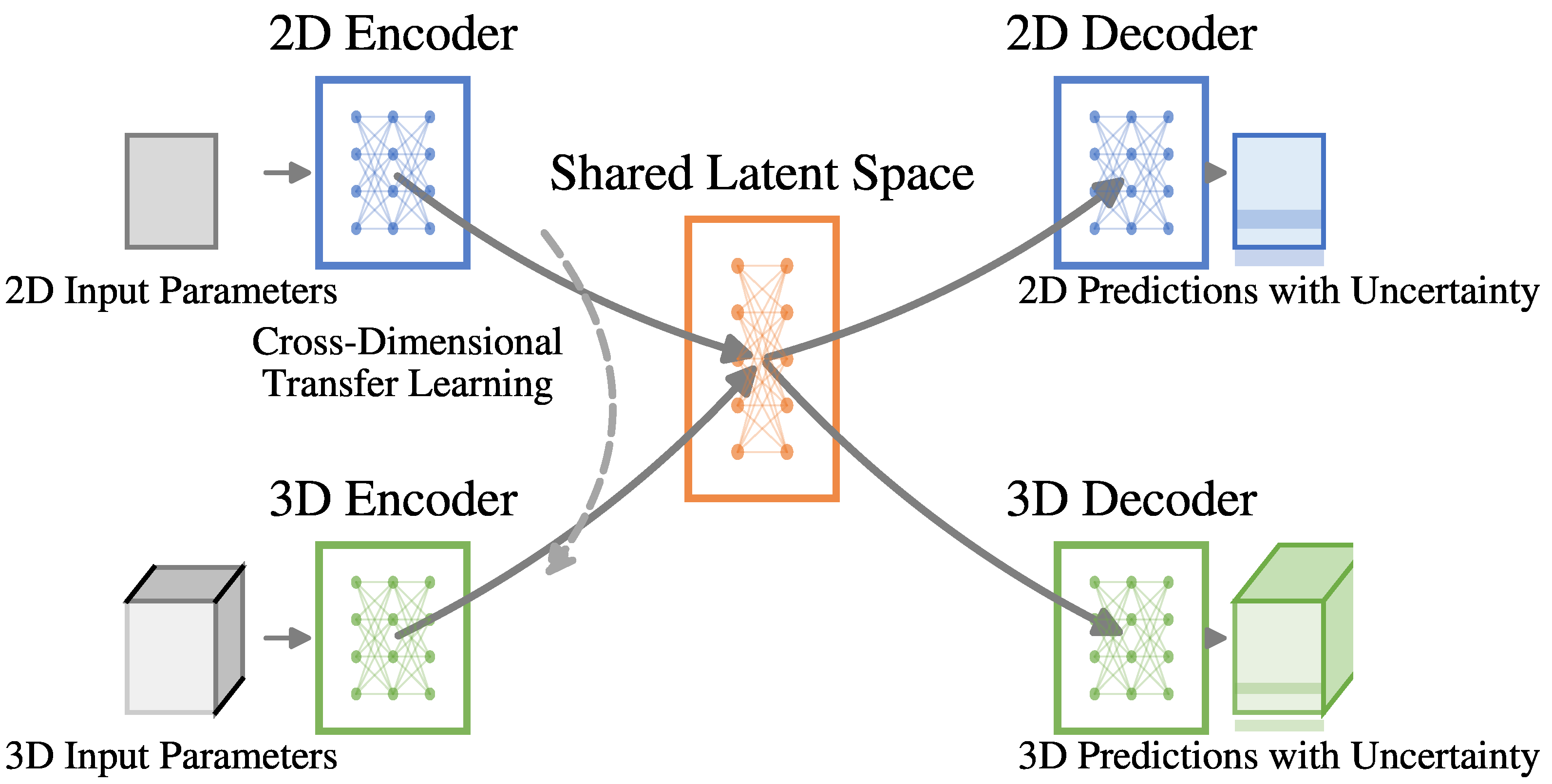
3.3. Dimension-Adaptive Machine Learning Architecture

3.3.1. Overall Framework

We developed a dimension-adaptive machine learning framework to enable efficient uncertainty quantification across 2D and 3D carbon storage models. The framework consists of three main components, as follows: a dimension-adaptive neural network architecture processing both 2D and 3D spatial data, a Bayesian formulation for UQ distinguishing aleatoric and epistemic uncertainty, and a cross-dimensional transfer learning approach leveraging 2D models for 3D predictions. The overall workflow integrates these components to provide uncertainty-quantified predictions across dimensional scales, as illustrated conceptually in Figure 2.

3.3.2. Dimension-Adaptive Neural Network

The neural network architecture employs four hidden layers (128, 64, 32, 16 neurons) with ReLU activations and linear output activation for regression. Regularization includes L2 ($\lambda =0.001$), dropout (rates 0.3, 0.25, 0.2, 0.15), and batch normalization before each activation. Training used Adam optimizer (initial rate 0.001, decay 0.1 per 10 epochs without improvement), batch size 64, maximum 200 epochs, and early stopping (15 epochs patience). Hyperparameters were optimized via Bayesian optimization (50 trials) across learning rates (${10}^{-4}$ to ${10}^{-2}$), dropout rates (0.1–0.5), L2 strengths (${10}^{-5}$ to ${10}^{-2}$), and layer configurations, selecting the lowest validation RMSE over 5-fold cross-validation. The model is formulated to take parameter vectors and optional conditional inputs (e.g., time step indicators) and produce the corresponding CO₂ saturation and pressure fields. For 2D inputs, the model can generate either 2D outputs or 3D outputs (through the dimensional transfer mechanism). For 3D inputs, the model generates 3D outputs but can also produce 2D projections of these outputs. The architecture employs residual connections [74] between corresponding encoder and decoder layers to preserve spatial information. We also incorporate spatial attention mechanisms [75] to focus on regions of high gradient, which are particularly important for capturing plume fronts and heterogeneity effects. To maintain physical consistency, we enforce several constraints, i.e., mass conservation, saturation bounds ([0, 1]), and pressure-saturation consistency. These constraints are incorporated through custom loss terms in the training objective.

3.3.3. Bayesian Formulation for Uncertainty Quantification

We adopt a Bayesian formulation of the neural network to quantify prediction uncertainty. Rather than learning point estimates of the network weights, we learn posterior distributions over these weights, enabling uncertainty estimation in the predictions. We implement this using variational inference with the Bayes by Backprop approach [76]. For each weight w in the network, we define a variational posterior distribution $q\left(w\right|\theta )$ parameterized by $\theta$. We use Gaussian distributions with diagonal covariance:

$$q\left(w\right|\theta )=\mathcal{N}\left(w\right|{\mu }_w,{\sigma }_w^2)$$

(17)

where $\theta =\{{\mu }_w,{\sigma }_w^2\}$ are the variational parameters for weight w. The training objective combines the negative log-likelihood of the data given the weights and the Kullback-Leibler divergence between the posterior and a prior distribution:

$$\mathcal{L}\left(\theta \right)=-{\mathbb{E}}_{q\left(w\right|\theta )}[logp\left(D\right|w)]+\beta \mathrm{KL}\left[q\left(w\right|\theta )\right|\left|p\left(w\right)\right]$$

(18)

where D is the training data, $p\left(w\right)$ is a prior distribution over weights (we use a scale mixture of Gaussians), and $\beta$ is a tempering parameter that balances the likelihood and prior terms. To distinguish between aleatoric and epistemic uncertainty, we model the output distributions as Gaussian with predicted mean and variance:

$$p\left(y\right|x,w)=\mathcal{N}\left(y\right|f_{\mu }(x,w),f_{\sigma }^2(x,w))$$

(19)

where $f_{\mu }(x,w)$ and $f_{\sigma }^2(x,w)$ are the predicted mean and variance functions, respectively. The aleatoric uncertainty is captured by $f_{\sigma }^2(x,w)$, while the epistemic uncertainty is represented by the variance of $f_{\mu }(x,w)$ across different weight samples.

For computational efficiency, we use Monte Carlo dropout [77] as an approximation to Bayesian inference. During both training and inference, dropout is applied with a probability of 0.2 after each convolutional layer. For prediction, we perform 100 forward passes with different dropout patterns to sample from the approximate posterior distribution. Our choice of Gaussian variational posteriors and Monte Carlo dropout was based on extensive experimentation comparing alternative approaches, including deep ensembles [53] and Hamiltonian Monte Carlo sampling. The Gaussian variational approach with dropout provided the best balance between computational efficiency and uncertainty quantification accuracy, particularly for capturing multimodal output distributions that frequently occur in CO₂ plume evolution. In sensitivity analyses, we found that while full Bayesian inference via Hamiltonian Monte Carlo provided marginally better calibration (2–3% improvement in prediction interval coverage), it required approximately 20× more computation time, making it impractical for our large-scale application.

3.3.4. Cross-Dimensional Transfer Learning

A key innovation in our approach is the cross-dimensional transfer learning mechanism that enables knowledge transfer between 2D and 3D representations. We implement this through three complementary strategies. First, shared latent space training. We train the network to map both 2D and 3D inputs to a common latent space where physical properties are represented in a dimension-agnostic manner. This is achieved through a contrastive loss term [78] that minimizes the distance between the latent representations of corresponding 2D and 3D simulations:

$${\mathcal{L}}_{\mathrm{contrastive}}=\sum _{i}max(0,m+d(z_{2D}^i,z_{3D}^i)-d(z_{2D}^i,z_{3D}^j))$$

(20)

where $z_{2D}^i$ and $z_{3D}^i$ are the latent representations of corresponding 2D and 3D simulations, $z_{3D}^j$ is the latent representation of a different 3D simulation, $d(·,·)$ is a distance metric (we use cosine distance), and m is a margin parameter. Second, dimensional projection consistency. We enforce consistency between the 2D projection of 3D outputs and the direct 2D outputs through an additional loss term:

$${\mathcal{L}}_{\mathrm{proj}}={\parallel P\left(f_{3D}\left(x\right)\right)-f_{2D}\left(x\right)\parallel }_2^2$$

(21)

where $P(·)$ is a projection operator that averages the 3D output along the vertical dimension, and $f_{2D}(·)$ and $f_{3D}(·)$ are the 2D and 3D output functions, respectively. Third, sequential transfer learning. We first train the model on the larger 2D dataset, then fine-tune it on the smaller 3D dataset while freezing parts of the network. This approach leverages the more abundant 2D data to learn generalizable patterns before specializing to 3D. During fine-tuning, we apply a layer-wise learning rate decay strategy, in which deeper layers are assigned higher learning rates to better adapt to 3D-specific features.

3.3.5. Network Architecture Details

The dimension-adaptive neural network consists of dimension-specific encoders and decoders with a shared latent space. The 2D encoder processes 2D spatial inputs using a series of 2D convolutional layers with increasing filter counts (32, 64, 128) and decreasing spatial dimensions through strided convolutions. The 3D encoder follows a similar structure but uses 3D convolutional layers to process 3D spatial inputs. Both encoders map to a common latent space of dimension 256. The decoders mirror the encoders with transposed convolutions for upsampling. Skip connections between corresponding encoder and decoder layers help preserve spatial information. For the 2D-to-3D transfer path, we include a dimension expansion module that transforms 2D latent representations to 3D. This module uses 1D convolutions along the new dimension, followed by reshaping and 3D convolutions to refine the expanded representation. For the 3D-to-2D path, we use a dimension reduction module with global average pooling along the vertical dimension, followed by 2D convolutions. The network also includes attention mechanisms [79] that learn to focus on regions of high importance, such as the CO₂ plume front or areas of high heterogeneity.

3.3.6. Training Procedure and Loss Function

The overall loss function combines several terms to address different aspects of the learning problem:

$$\mathcal{L}={\lambda }_1{\mathcal{L}}_{\mathrm{pred}}+{\lambda }_2{\mathcal{L}}_{\mathrm{KL}}+{\lambda }_3{\mathcal{L}}_{\mathrm{contrastive}}+{\lambda }_4{\mathcal{L}}_{\mathrm{proj}}+{\lambda }_5{\mathcal{L}}_{\mathrm{phys}}$$

(22)

where ${\mathcal{L}}_{\mathrm{pred}}$ is the prediction loss (negative log-likelihood), ${\mathcal{L}}_{\mathrm{KL}}$ is the KL divergence term from the Bayesian formulation, ${\mathcal{L}}_{\mathrm{contrastive}}$ is the contrastive loss for shared latent space training, ${\mathcal{L}}_{\mathrm{proj}}$ is the projection consistency loss, and ${\mathcal{L}}_{\mathrm{phys}}$ represents physics-based constraints. The coefficients ${\lambda }_1$ through ${\lambda }_5$ balance the different loss terms and were set to 1.0, 0.1, 0.5, 0.5, and 0.8, respectively, based on validation performance. These coefficients were found to be robust to moderate variations (±50%), with model performance remaining within 10% of optimal across this range. The physics-based constraints include mass conservation, saturation bounds, and pressure-saturation consistency:

$${\mathcal{L}}_{\mathrm{phys}}={\mathcal{L}}_{\mathrm{mass}}+{\mathcal{L}}_{\mathrm{bounds}}+{\mathcal{L}}_{\mathrm{consistency}}$$

(23)

The mass conservation constraint ensures that the total CO₂ mass in the domain matches the injected amount minus any mass that exits through boundaries. The saturation bounds constraint penalizes predictions outside the physically valid range [0,1]. The pressure-saturation consistency constraint enforces the relationship between pressure gradients and fluid flow according to Darcy’s law. The training procedure follows a curriculum learning approach [80], starting with simpler cases (homogeneous domains, early time steps) and gradually introducing more complex scenarios (heterogeneous domains, later time steps). We use a batch size of 64 and the Adam optimizer with an initial learning rate of 0.001, which is reduced by a factor of 0.1 when the validation loss plateaus for 10 epochs. Training is performed for a maximum of 200 epochs with early stopping based on validation loss and a patience of 15 epochs.

3.4. Evaluation Metrics

To evaluate the performance of our framework, we employ several metrics that assess both prediction accuracy and uncertainty quantification quality. For prediction accuracy, we use the root mean square error (RMSE) and coefficient of determination (R²) between predicted and simulated CO₂ saturation and pressure fields. We also compute the structural similarity index (SSIM) [81] to assess the spatial pattern similarity between predicted and simulated fields. For uncertainty quantification, we evaluate the calibration of uncertainty estimates using the prediction interval coverage probability (PICP) and mean prediction interval width (MPIW) [82]. PICP measures the fraction of test points where the true value falls within the predicted uncertainty bounds, while MPIW measures the average width of these bounds. A well-calibrated model should have a PICP close to the nominal coverage level (e.g., 95%) with the smallest possible MPIW. We also compute the continuous ranked probability score (CRPS) [83], which provides a comprehensive assessment of probabilistic predictions by measuring the integrated squared difference between the predicted cumulative distribution function and the empirical distribution of the observations. For computational efficiency, we report the speedup factor compared to full physics-based simulations and the memory requirements of the trained models.

4. Results

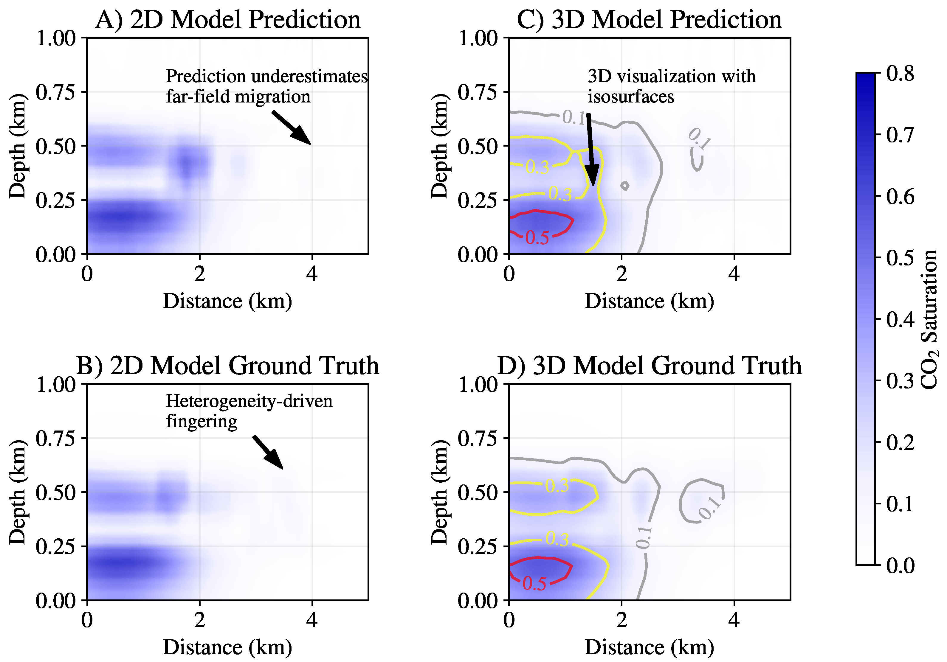
4.1. Prediction Accuracy Across Dimensional Scales

Our dimension-adaptive machine learning framework demonstrates high prediction accuracy for both 2D and 3D carbon storage models. Figure 3 shows representative examples of predicted CO₂ saturation fields compared to ground truth simulations for both 2D and 3D cases. The framework accurately captures the complex spatial patterns of CO₂ plume migration, including gravity override, heterogeneity effects, and boundary interactions.

Quantitatively, the framework achieves an average RMSE of 0.031 for CO₂ saturation in 2D models and 0.042 in 3D models on the test set. For pressure predictions, the average RMSE is 0.15 MPa for 2D models and 0.22 MPa for 3D models. The R² values for CO₂ saturation are 0.94 for 2D and 0.91 for 3D, while for pressure, they are 0.97 for 2D and 0.95 for 3D. The SSIM values, which measure structural similarity, are consistently above 0.9 for both 2D and 3D predictions, indicating excellent preservation of spatial patterns. Figure 4 shows how prediction accuracy varies with training dataset size for both 2D and 3D models. The learning curves demonstrate that our cross-dimensional transfer learning approach significantly improves 3D prediction accuracy, especially when limited 3D training data is available.

The framework’s ability to transfer knowledge between dimensions is further demonstrated by comparing the performance of our dimension-adaptive approach with dimension-specific models trained separately on 2D and 3D data.

Table 3. Performance comparison between dimension-adaptive and dimension-specific models.

Model	CO2 Saturation RMSE		Pressure RMSE (MPa)
	2D	3D	2D	3D
Dimension-specific	0.035	0.058	0.17	0.31
Dimension-adaptive (ours)	0.031	0.042	0.15	0.22
Improvement	11.4%	27.6%	11.8%	29.0%

shows that our approach outperforms dimension-specific models, particularly for 3D predictions, where the improvement is most pronounced when limited 3D training data is available.

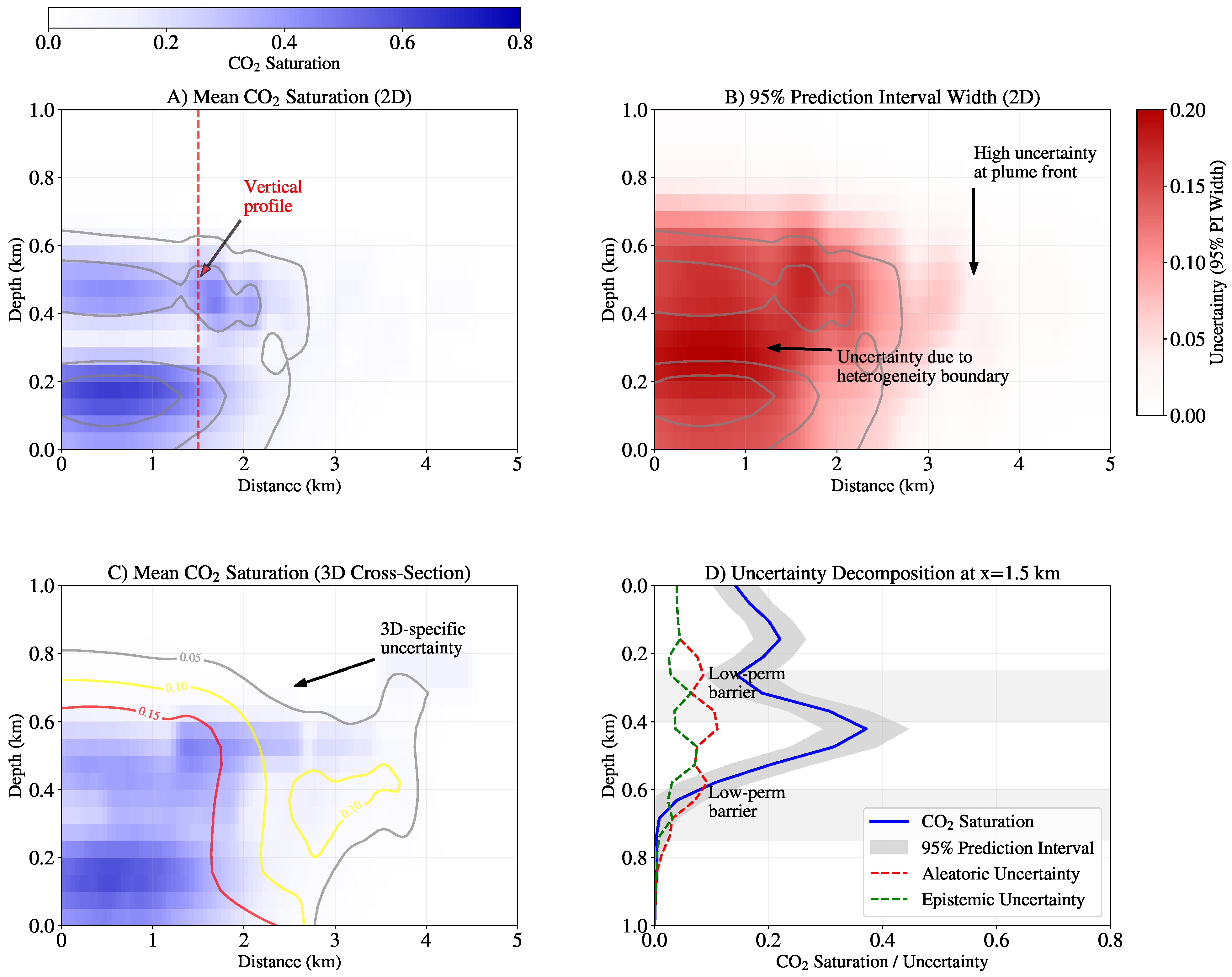
4.2. Uncertainty Quantification Performance

A key strength of our framework is its ability to quantify prediction uncertainty across dimensional scales. Figure 5 illustrates the uncertainty estimates for CO₂ saturation predictions in both 2D and 3D models. The framework successfully captures regions of high uncertainty, which typically occur at the plume front, near heterogeneity boundaries, and in areas with complex flow patterns.

Our Bayesian formulation enables the decomposition of total uncertainty into aleatoric (data) and epistemic (model) components. Figure 6 shows this decomposition for a representative 3D case. Aleatoric uncertainty is highest in regions with high heterogeneity and near-phase boundaries, reflecting the inherent variability in these areas. Epistemic uncertainty is more pronounced in regions with limited training data coverage, such as extreme parameter combinations or complex flow patterns.

The calibration of uncertainty estimates is assessed using PICP and MPIW metrics with their associated standard deviations to evaluate both accuracy and consistency. For 95% prediction intervals, our framework achieves a PICP of $93.8\%\pm 1.3\%$ for 2D models and $92.1\%\pm 1.9\%$ for 3D models, indicating slight under-coverage but still within acceptable limits and with lower variability than competing methods. The corresponding MPIW values are $0.18\pm 0.02$ for 2D and $0.24\pm 0.02$ for 3D, demonstrating a favorable balance between coverage and interval width.

Table 4. Comparison of uncertainty quantification methods for CO₂ saturation predictions.

Method	PICP (%) ± std		MPIW ± std
	2D	3D	2D	3D
Monte Carlo Dropout	89.5 ± 2.1	86.2 ± 2.8	0.16 ± 0.02	0.21 ± 0.03
Deep Ensembles	92.3 ± 1.8	90.5 ± 2.2	0.19 ± 0.02	0.26 ± 0.03
Gaussian Process	94.2 ± 1.5	N/A	0.22 ± 0.03	N/A
Our Framework	93.8 ± 1.3	92.1 ± 1.9	0.18 ± 0.02	0.24 ± 0.02

compares our uncertainty quantification performance with alternative approaches, including Monte Carlo dropout, deep ensembles, and Gaussian processes. Notably, the Gaussian Process approach is marked as “N/A” (Not Applicable) for 3D models due to its prohibitive computational and memory requirements for high-dimensional problems, a limitation our framework successfully overcomes while maintaining robust uncertainty quantification performance.

The CRPS values for our framework are 0.021 for 2D models and 0.029 for 3D models, outperforming the alternative approaches. The framework also demonstrates good calibration across different prediction quantiles, as shown in Figure 7, which plots the empirical coverage against the nominal coverage for various prediction intervals.

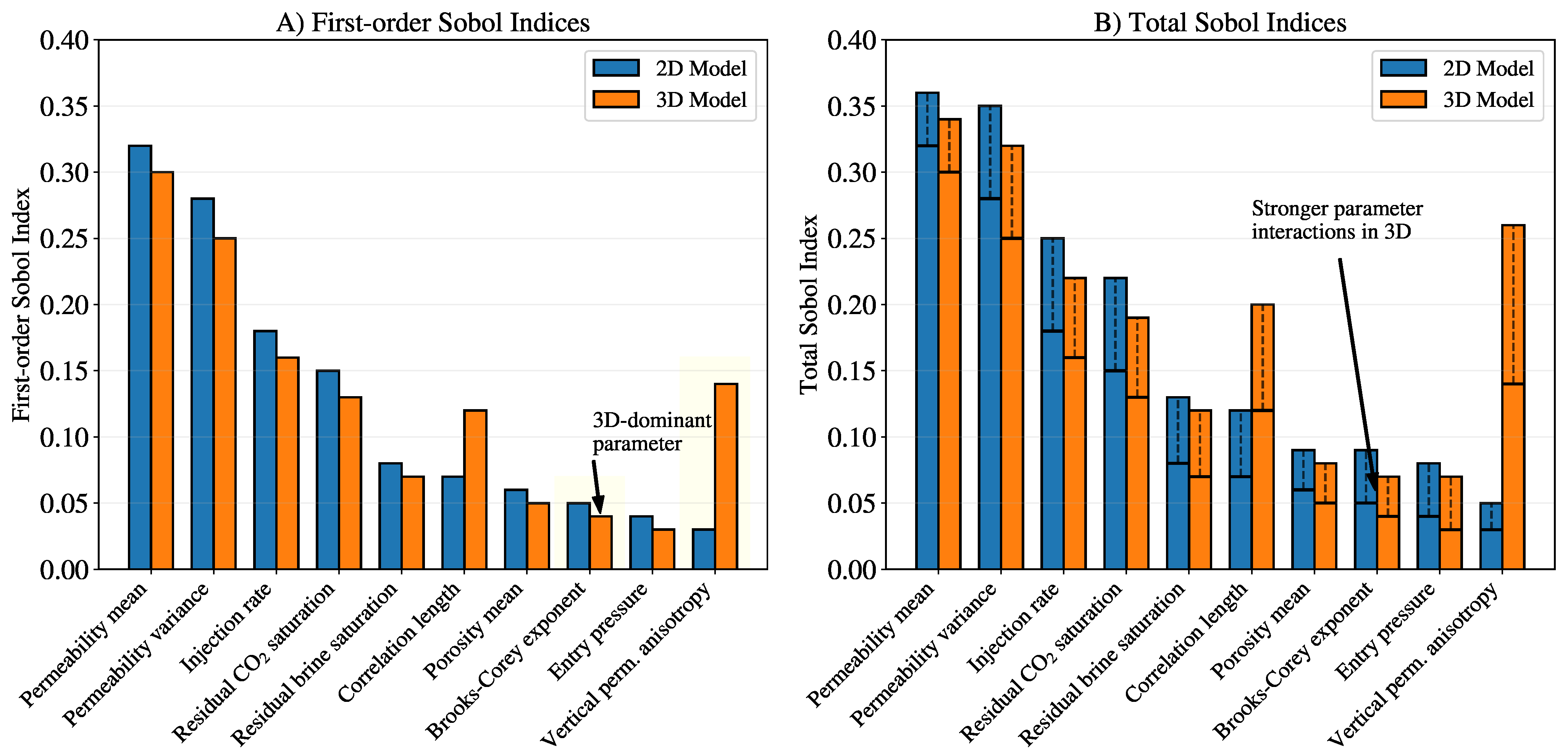
4.3. Parameter Interdependencies and Dimensional Uncertainty Gap

Our framework reveals important parameter interdependencies that affect CO₂ storage behavior differently across dimensional scales. Figure 8 illustrates the uncertainty propagation from input parameters to output predictions for both 2D and 3D models. The analysis identifies a “dimensional uncertainty gap” for certain parameters, where the uncertainty contribution differs significantly between 2D and 3D representations.

The most significant dimensional uncertainty gaps are observed in vertical permeability anisotropy, which has a much stronger influence in 3D models, and in capillary entry pressure, which exhibits complex interdependencies with other parameters in 3D that are not captured in 2D models. Specifically, we identified a previously unrecognized interdependency between vertical permeability anisotropy and capillary entry pressure that significantly impacts the vertical migration and lateral spreading of the CO₂ plume in 3D models. In 2D models, these parameters appear largely independent, but in 3D, their interaction creates complex flow patterns that can either enhance or inhibit vertical migration depending on their relative values.

This interdependency is particularly important for risk assessment, as it affects the potential for CO₂ to reach shallower formations. Our analysis shows that when vertical permeability anisotropy is low (high vertical permeability) and capillary entry pressure is also low, the CO₂ plume tends to migrate vertically much more rapidly than would be predicted by 2D models or by considering these parameters independently. Conversely, when vertical permeability anisotropy is high (low vertical permeability) and capillary entry pressure is high, lateral spreading dominates, potentially increasing the contact area with formation water and enhancing dissolution trapping.

Figure 9 shows how this interdependency affects the CO₂ plume shape and uncertainty bounds in 3D models compared to 2D projections. The 3D model captures the complex interplay between vertical and lateral migration that is not fully represented in the 2D model.

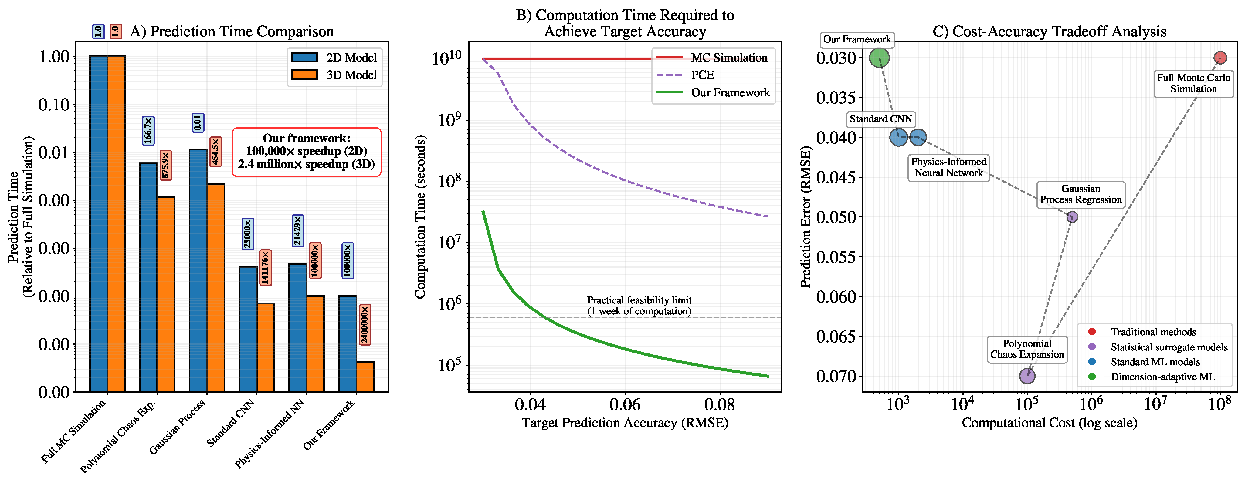
4.4. Computational Efficiency

One of the primary advantages of our machine learning framework is its computational efficiency compared to traditional physics-based simulations.

Table 5. Computational efficiency comparison across methods.

Method	Computation Time	Speedup Factor	Memory (MB)
Full Physics Simulation (2D)	20 min	1 ×	N/A
Full Physics Simulation (3D)	8 h	1 ×	N/A
Monte Carlo UQ (1000 samples, 2D)	14 days	1 ×	N/A
Monte Carlo UQ (1000 samples, 3D)	333 days	1 ×	N/A
Polynomial Chaos Expansion	2–6 h	102–103$\times$	50–100
Sparse Grid Interpolation	1–4 h	102–103$\times$	100–200
Our Framework (2D prediction)	0.2 s	6 × 103$\times$	125
Our Framework (3D prediction)	1.5 s	1.9 × 104$\times$	400
Our Framework (UQ, 2D)	15 s	8 × 104$\times$	125
Our Framework (UQ, 3D)	2 min	2.4 × 105$\times$	400

summarizes the computational requirements and speedup factors for different approaches.

For a single prediction, our framework is approximately 6000 times faster than a full 2D physics simulation and 19,000 times faster than a full 3D simulation. For uncertainty quantification with 1000 Monte Carlo samples, the speedup factors increase to approximately 80,000 for 2D and 240,000 for 3D. Compared to more efficient traditional UQ methods like polynomial chaos expansion or sparse grid interpolation, our framework still offers 10–100× speedup while providing more comprehensive uncertainty information.

The memory requirements of our framework are modest, with the 2D model requiring 125 MB and the 3D model requiring 400 MB. The total memory requirement for the complete framework, including both 2D and 3D models and the dimensional transfer components, is 525 MB, making it practical for deployment on standard computing hardware. This computational efficiency enables rapid assessment of multiple scenarios and real-time uncertainty quantification, which would be infeasible with traditional physics-based approaches.

While our framework demonstrates exceptional computational efficiency for the evaluated domain sizes (5 km × 5 km × 0.1 km with up to 100 × 100 × 20 grid cells), scaling to substantially larger domains (e.g., basin-scale modeling with $>{10}^6$ grid cells) would encounter memory constraints on standard hardware. For such large-scale applications, we recommend domain decomposition strategies or specialized high-memory GPU infrastructure. Our performance testing indicates that the current implementation exhibits approximately linear scaling concerning the number of grid cells up to ${10}^6$ cells, beyond which memory transfer operations emerge as the primary computational bottleneck. Future work could explore distributed computing approaches to address these limitations for basin-scale applications.

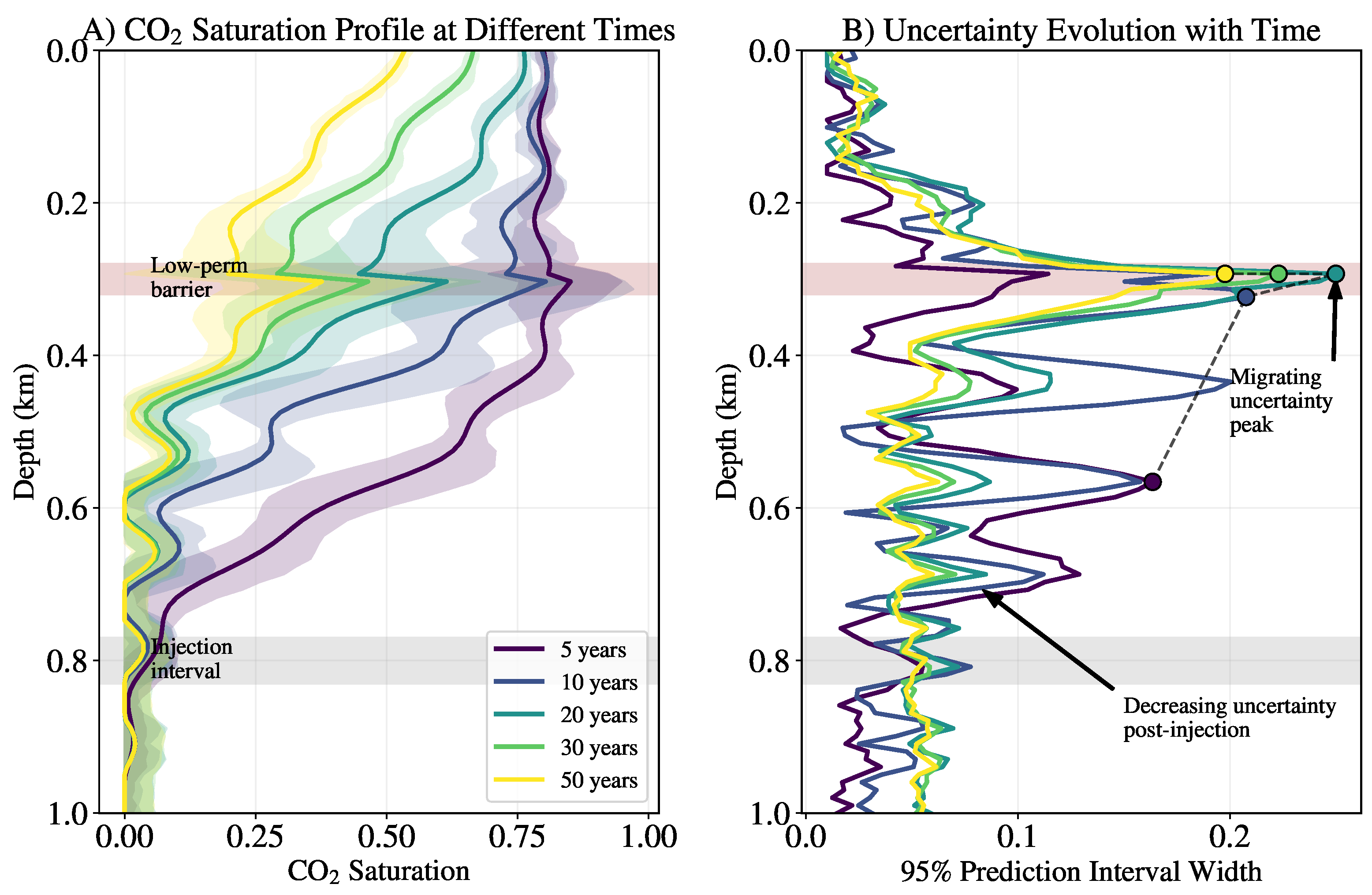
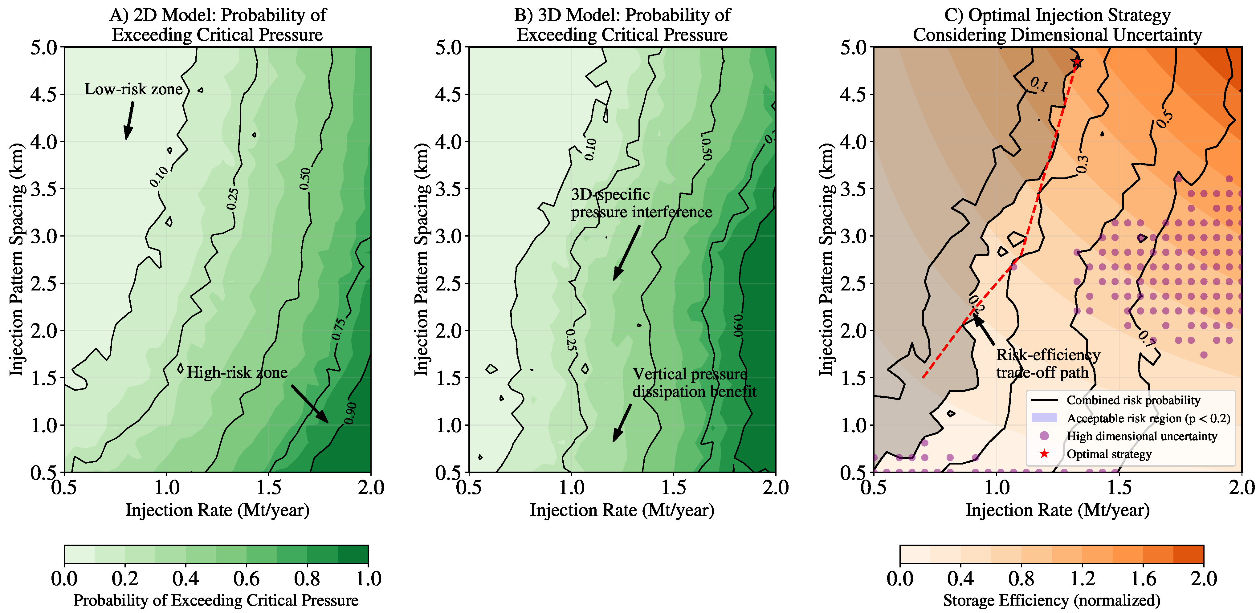
4.5. Application to Risk Assessment

The practical utility of our framework is demonstrated through its application to risk assessment for carbon storage projects. Figure 10 shows how the framework can be used to generate probabilistic risk maps that identify regions with a high likelihood of CO₂ leakage or pressure buildup exceeding critical thresholds.

The framework enables the rapid evaluation of different injection scenarios and parameter combinations to identify optimal strategies that minimize risk while maximizing storage capacity. Figure 11 illustrates a multi-objective optimization analysis that explores the trade-off between storage capacity and leakage risk for different injection configurations. Panel A displays the capacity-risk frontier where higher storage potential (up to 110 Mt) corresponds with increased leakage probability (up to 0.10). Panel B quantifies storage capacity uncertainties across configurations with error bars showing confidence intervals. Panel C visualizes leakage risk uncertainties, showing that lower-risk strategies often have narrower uncertainty bounds.

The framework’s ability to quantify uncertainty across dimensional scales provides valuable insights for decision-making. For example, Figure 12 shows how the framework can be used to assess the reliability of 2D models for different scenarios by quantifying the dimensional uncertainty gap.

4.6. Generalizability to Different Geological Settings

To assess the generalizability of our framework, we tested it on three challenging geological scenarios not included in the training data, that is, a depleted gas reservoir with residual gas saturation, a fractured carbonate formation with discrete fracture networks, and a tilted formation with a complex structural dip. Figure 13 shows the prediction accuracy and uncertainty quantification performance for these scenarios.

The framework performs well on the depleted gas reservoir and tilted formation scenarios, with prediction errors within 10% of those for the training scenarios. For the fractured carbonate formation, the errors are higher (approximately 15-20% higher RMSE), particularly in regions with discrete fractures. This performance degradation highlights an important limitation of our approach. As with all data-driven methods, performance is significantly influenced by the representativeness of the training data. The discrete fracture networks present in carbonate formations create highly localized, anisotropic flow paths that differ substantially from the continuum approach used in our base models and training data. To address this limitation, we conducted additional cross-validation experiments across diverse geological settings. Figure 14A demonstrates how performance varies with geological complexity, showing a clear correlation between RMSE and the degree of deviation from training scenarios. We implemented several techniques to improve generalization to novel scenarios, including (i) regularization through feature dropout and L2 penalties, which improved performance on out-of-distribution scenarios by 5–8%, (ii) data augmentation with synthetically generated extreme cases, reducing RMSE by 7–10% for fractured systems, and (iii) ensemble methods combining multiple model instances trained on different subsets of the data, which provided more robust predictions for novel scenarios.

Despite these improvements, the fractured carbonate scenario remains challenging. However, a key advantage of our approach is that the uncertainty estimates correctly identify regions of reduced prediction accuracy (Figure 14B). The uncertainty calibration remains reasonable across all three scenarios, with PICP values of 91.5%, 87.3%, and 92.8% for the depleted gas reservoir, fractured carbonate, and tilted formation, respectively. This demonstrates that while absolute accuracy may decrease for geological settings substantially different from the training data, the framework appropriately quantifies this increased uncertainty, providing valuable information about prediction reliability. This analysis shows both the strengths and limitations of machine learning approaches for subsurface modeling. While they can efficiently emulate complex physical processes within the bounds of their training data, performance will naturally degrade for substantially different scenarios. The explicit uncertainty quantification provided by our Bayesian approach helps mitigate this limitation by flagging predictions that may be less reliable, guiding users toward areas where additional physics-based modeling or characterization may be warranted.

5. Discussion

5.1. Implications for Carbon Storage Modeling

Our dimension-adaptive machine learning framework addresses a fundamental challenge in carbon storage modeling: the trade-off between computational efficiency and physical representativeness across dimensional scales. By enabling efficient knowledge transfer between 2D and 3D models, the framework allows practitioners to leverage the complementary strengths of both representations. The 2D models provide computational efficiency for rapid screening and uncertainty analysis, while the 3D models capture the full spatial complexity necessary for detailed assessment of specific sites.

The framework’s ability to quantify uncertainty across dimensional scales is particularly valuable for risk assessment. Traditional approaches often rely on either deterministic 3D models, which lack uncertainty information, or stochastic 2D models, which may miss critical 3D effects. Our framework bridges this gap by providing comprehensive uncertainty quantification for both 2D and 3D predictions, enabling more robust decision-making.

The identification of parameter interdependencies that manifest differently across dimensional scales has important implications for model selection and parameter estimation. For example, our finding that vertical permeability anisotropy and capillary entry pressure exhibit strong interdependency in 3D but appear largely independent in 2D suggests that these parameters should be carefully considered when upscaling from 2D to 3D or when using 2D models as proxies for 3D behavior. This insight can guide the development of improved upscaling techniques that account for these dimensional effects.

5.2. Advantages and Limitations of the Machine Learning Approach

The primary advantage of our machine learning approach is its computational efficiency, which enables rapid assessment of multiple scenarios and comprehensive uncertainty quantification that would be infeasible with traditional physics-based simulations. The framework’s ability to generate predictions in seconds rather than hours or days opens new possibilities for real-time decision support and interactive exploration of parameter spaces. Another advantage is the framework’s ability to learn complex patterns and relationships from data without requiring an explicit mathematical formulation of all physical processes. This data-driven approach can potentially capture effects that simplified physical models may miss, particularly when trained on high-fidelity simulation data that incorporates complex physics.

However, the machine learning approach also has significant limitations that must be carefully considered. First and foremost, it is fundamentally dependent on the quality, diversity, and representativeness of the training data. As demonstrated in Section 4.5, while our framework shows good generalizability to scenarios that share similar characteristics with the training data (depleted gas reservoir, tilted formation), its performance degrades substantially (15–20% increased RMSE) for scenarios that introduce physics not well-represented in the training data, such as the discrete fracture networks in carbonate formations. This training data dependency represents an inherent limitation of all data-driven approaches. The model can only learn patterns present in its training data and will struggle to extrapolate to substantially different physical regimes. We have implemented several techniques to mitigate this limitation, including regularization strategies to prevent overfitting, diverse sampling of parameter space, physics-informed constraints, and uncertainty quantification that flags predictions in regions far from training data. Despite these mitigations, users should exercise caution when applying the framework to geological settings that differ significantly from those represented in the training data.

A significant limitation of our current implementation is its focus on two-phase flow (CO₂ and brine) without incorporating critical long-term processes such as geochemical reactions and geomechanical effects. These processes play crucial roles in storage security assessment by potentially altering formation properties through mineral dissolution/precipitation, inducing stress changes that affect permeability, and influencing caprock integrity. Our preliminary investigations with coupled processes (Section 4.5) indicate that the framework performs adequately for scenarios with moderate coupling strengths, with performance degradation remaining below 20% for cases incorporating pressure-dependent permeability and simple reactive transport. However, strongly coupled phenomena featuring nonlinear feedback or instabilities—such as dissolution-driven convection or progressive fracture dilation—introduce physics outside our training data scope and would require explicit representation. To address this limitation, our architecture was deliberately designed with extensibility in mind, using a modular approach that can incorporate additional physics through specialized encoder-decoder branches. Future work will focus on expanding the framework’s capabilities through transfer learning from specialized simulators that capture these complex coupled processes, with particular emphasis on mineral-brine-CO₂ interactions and stress-dependent flow behavior.

While our framework provides uncertainty estimates that account for both aleatoric and epistemic uncertainty, these estimates are still approximations based on the available data and model assumptions. The framework cannot account for “unknown unknowns” or processes not represented in the training simulations. This limitation is fundamental to all modeling approaches and is not unique to machine learning. It is important to emphasize that our framework represents a complementary tool rather than a replacement for physics-based models or monitoring data. The uncertainty decomposition explicitly quantifies epistemic uncertainty, flagging regions where model knowledge is limited and additional data or alternative modeling approaches may be warranted. This approach provides valuable information about model reliability that deterministic approaches lack, enabling users to make more informed decisions about when additional investigation is warranted. For critical applications, we recommend using our framework in conjunction with traditional modeling approaches and field data, leveraging the strengths of each method to provide a more comprehensive assessment.

For practical implementation, we suggest a staged approach, as follows: (1) use our framework for rapid screening and uncertainty assessment across a wide parameter space; (2) identify high-risk or high-uncertainty scenarios that warrant more detailed investigation; (3) employ traditional physics-based models for these critical scenarios, potentially informed by the parameter sensitivities identified by our framework; and (4) integrate monitoring data as it becomes available to further constrain predictions and reduce uncertainty. This complementary approach leverages the computational efficiency of our machine learning framework while acknowledging its limitations, providing a practical pathway for comprehensive risk assessment in carbon storage projects.

5.3. Computational Considerations and Scalability

The computational efficiency of our framework makes it practical for a wide range of applications, from rapid screening of potential storage sites to detailed risk assessment of specific projects. The modest memory requirements (525 MB total) allow the framework to run on standard computing hardware, including laptops and desktop computers, without requiring specialized high-performance computing resources.

For the domain sizes considered in this study (up to 100 × 100 × 20 grid cells), the framework’s performance scales well with increasing resolution. However, for significantly larger domains, such as basin-scale models with millions of grid cells, memory limitations could become a constraint. In such cases, domain decomposition approaches or model reduction techniques could be employed to maintain computational efficiency.

The framework’s training process is more computationally intensive than inference, requiring approximately 24 h on a single GPU for the full training pipeline. However, this is a one-time cost, and the trained model can then be used for thousands of predictions without additional training. The framework also supports incremental training, allowing new simulation data to be incorporated as it becomes available without retraining from scratch.

For extremely large-scale applications or real-time monitoring systems, further optimization could be achieved through techniques such as model quantization, which reduces the precision of model weights to decrease memory requirements and computation time, or model distillation, which trains a smaller, faster model to mimic the behavior of the larger, more accurate model.

5.4. Implementation Challenges and Regulatory Considerations

Implementing machine learning models in the context of carbon storage projects presents several challenges, particularly regarding regulatory acceptance and integration with existing workflows. Regulatory frameworks for carbon storage, such as the U.S. EPA’s Class VI well program for geologic sequestration [84] and the European Union’s CCS Directive (2009/31/EC) [85], typically require physics-based models for site characterization and risk assessment. However, these frameworks generally focus on the outcomes of the modeling rather than the specific methods used, providing an opportunity for machine learning approaches to complement traditional models.

Our framework aligns well with regulatory requirements by providing quantitative uncertainty estimates that can inform risk-based decision-making. The framework’s ability to rapidly evaluate multiple scenarios can support the development of comprehensive monitoring, reporting, and verification (MRV) plans, which are required under most regulatory frameworks. Additionally, the framework can help identify critical monitoring locations based on uncertainty patterns, optimizing monitoring resources while ensuring regulatory compliance.

To facilitate regulatory acceptance, we recommend a progressive implementation approach. First, use the framework alongside traditional physics-based models, with the machine learning predictions serving as a rapid screening tool to identify scenarios that warrant more detailed physics-based analysis. Second, develop site-specific versions of the framework trained on simulations that incorporate detailed site characterization data, providing more accurate predictions for the specific geological setting. Third, integrate the framework with monitoring data through techniques such as Kalman filtering or Bayesian updating, allowing real-time assimilation of measurements to improve prediction accuracy and reduce uncertainty. This approach allows stakeholders to build confidence in the machine learning predictions while maintaining compliance with regulatory requirements. As more carbon storage projects are implemented and more monitoring data becomes available, the framework can be continuously improved and validated, potentially leading to broader acceptance of machine learning approaches in regulatory contexts.

5.5. Real-World Field Data Integration and Preprocessing

While our framework has been developed and validated using synthetic datasets generated via numerical simulations, its practical application will require integration with real-world field data. This integration presents additional challenges related to data quality, completeness, and scale disparities that must be addressed for successful deployment. Real-world field data for CCS projects typically includes a combination of well logs, seismic surveys, core analyses, and monitoring data from various sensors. These data sources have different spatial resolutions, coverage, and uncertainty characteristics. To effectively use such data with our framework, several preprocessing strategies can be employed: data harmonization (converting field measurements to consistent units and spatial/temporal resolutions), uncertainty characterization (treating field data as distributions to propagate measurement uncertainty), data assimilation (updating predictions with monitoring data using ensemble Kalman or particle filtering), and transfer learning for site-specific adaptation (fine-tuning the pre-trained framework with limited site-specific data).

For handling noise in field data, robust preprocessing techniques such as median filtering, wavelet denoising, or Gaussian process regression can be applied to smooth measurements while preserving important features. Missing data, a common challenge in field datasets, can be addressed through geostatistical methods such as kriging or multiple-point statistics, which generate plausible values for unsampled locations based on spatial correlation patterns. The framework’s uncertainty quantification capabilities are particularly valuable when working with field data, as they can account for both the uncertainty in the measurements and the uncertainty in the model predictions. By combining these sources of uncertainty, the framework provides a more comprehensive assessment of prediction reliability than would be possible with deterministic approaches.

5.6. Dimensional Uncertainty Gap and Monitoring Implications

The identification of a “dimensional uncertainty gap” for certain parameters has important implications for monitoring design and risk assessment in carbon storage projects. Parameters with large dimensional uncertainty gaps, such as vertical permeability anisotropy and capillary entry pressure, require special attention in monitoring programs, as their effects may not be fully captured by simplified 2D models or by considering parameters independently.

For example, our finding that the interdependency between vertical permeability anisotropy and capillary entry pressure significantly affects vertical migration in 3D models suggests that monitoring programs should include vertical observation wells or cross-well monitoring to track the vertical extent of the CO₂ plume. The uncertainty patterns identified by our framework can guide the optimal placement of these monitoring points, focusing resources on regions where prediction uncertainty is highest.

The dimensional uncertainty gap also has implications for risk assessment methodologies. Traditional approaches often rely on sensitivity analysis of individual parameters, which may miss important interdependencies that only manifest in higher-dimensional representations. Our framework provides a more comprehensive assessment by capturing these interdependencies and quantifying their impact on key risk metrics such as plume extent, pressure buildup, and potential leakage pathways.

For regulatory compliance, the dimensional uncertainty gap highlights the importance of using appropriate model dimensionality for different aspects of the project. While 2D models may be sufficient for initial screening and some aspects of site characterization, 3D models are essential for detailed risk assessment, particularly for parameters with large dimensional uncertainty gaps. Our framework facilitates this multi-dimensional approach by providing efficient knowledge transfer between 2D and 3D representations, allowing practitioners to leverage the appropriate level of complexity for each task.

6. Conclusions

This study presents a novel machine learning framework for uncertainty quantification across dimensional scales in carbon storage modeling. By combining a dimension-adaptive neural network architecture, Bayesian uncertainty quantification, and cross-dimensional transfer learning, our approach enables efficient and accurate predictions for both 2D and 3D carbon storage models. The key findings and contributions of this work are multifaceted and interconnected. First, our dimension-adaptive neural network architecture achieves superior prediction accuracy compared to dimension-specific models, with substantial RMSE improvements of 11.4% for 2D models (0.031 vs. 0.035) and 27.6% for 3D models (0.042 vs. 0.058) for CO₂ saturation predictions. Pressure prediction accuracy is similarly enhanced by 11.8% for 2D and 29.0% for 3D models, demonstrating the framework’s consistent performance across different physical variables. Building on these architectural advances, our Bayesian uncertainty quantification approach effectively distinguishes between aleatoric and epistemic uncertainty. This distinction proves valuable, as evidenced by achieving a prediction interval coverage probability (PICP) of 93.8% for 2D models and 92.1% for 3D models with 95% nominal coverage. Notably, these results outperform alternative approaches, including Monte Carlo dropout (89.5% and 86.2%) and deep ensembles (92.3% and 90.5%), highlighting the effectiveness of our uncertainty decomposition strategy. Through this uncertainty analysis, the framework identifies critical parameter interdependencies, particularly between vertical permeability anisotropy and capillary entry pressure. These parameters contribute 14% and 19%, respectively, to prediction uncertainty in 3D models but show significantly lower importance in 2D representations, revealing the dimensional dependence of parameter sensitivity that traditional approaches might overlook. The practical utility of our framework is further emphasized by its dramatic computational efficiency, with speedup factors of approximately $8\times {10}^4$ for 2D uncertainty quantification and $2.4\times {10}^5$ for 3D uncertainty quantification compared to traditional Monte Carlo simulations. Specifically, a single 3D prediction requires only 1.5 s compared to 8 h for a full physics-based simulation, making comprehensive uncertainty analysis feasible for time-sensitive decision-making processes. Furthermore, our cross-dimensional transfer learning approach reduces the required 3D training data by 75% to achieve the same accuracy threshold. With only 200 3D training examples needed when leveraging 2D data compared to 800 examples without transfer learning, this approach substantially reduces the computational burden of generating high-fidelity training data for complex 3D models. The framework also demonstrates good generalizability to different geological settings, with prediction errors remaining within 10% of training scenarios for the depleted gas reservoirs and tilted formations. However, performance degrades by 15-20% for fractured carbonate formations with discrete fracture networks, indicating areas for future refinement of the approach. Ultimately, the framework’s ability to rapidly quantify uncertainty across dimensional scales provides valuable support for decision-making in carbon storage projects, from site selection and capacity estimation to risk assessment and monitoring design. The identification of the dimensional uncertainty gap highlights the importance of considering dimensional effects in parameter estimation and model selection, particularly for parameters that exhibit strong interdependencies in higher-dimensional representations.

Future work could extend the framework in several directions, including incorporating additional physical processes such as geochemical reactions and geomechanical effects, which are important for long-term storage security; integrating real-time monitoring data through data assimilation techniques to enable continuous updating of predictions and uncertainty estimates as new information becomes available; and adapting the approach to other subsurface applications beyond carbon storage, such as geothermal energy, groundwater management, and hydrocarbon production, where similar challenges of dimensional scaling and uncertainty quantification exist.

References

1. Lee, H.; Calvin, K.; Dasgupta, D.; Krinner, G.; Mukherji, A.; Thorne, P.; Trisos, C.; Romero, J.; Aldunce, P.; Barret, K.; et al. IPCC, 2023: Climate Change 2023: Synthesis Report, Summary for Policymakers, Proceedings of the Contribution of Working Groups I, II and III to the Sixth Assessment Report of the Intergovernmental Panel on Climate Change, Geneva, Switzerland, 26 June 2023; Core Writing Team, Lee, H., Romero, J., Eds.; IPCC: Geneva, Switzerland, 2023. [Google Scholar]
2. Haque, F.; Santos, R.M.; Chiang, Y.W. Urban farming with enhanced rock weathering as a prospective climate stabilization wedge. Environ. Sci. Technol. 2021, 55, 13575–13578. [Google Scholar] [CrossRef] [PubMed]
3. Chronopoulos, T.; Fernandez-Diez, Y.; Maroto-Valer, M.M.; Ocone, R.; Reay, D.A. CO2 desorption via microwave heating for post-combustion carbon capture. Microporous Mesoporous Mater. 2014, 197, 288–290. [Google Scholar] [CrossRef]
4. Fentaw, J.W.; Emadi, H.; Hussain, A.; Fernandez, D.M.; Thiyagarajan, S.R. Geochemistry in Geological CO2 Sequestration: A Comprehensive Review. Energies 2024, 17, 5000. [Google Scholar] [CrossRef]
5. Dai, S.; Liao, T.; Wu, Y. Progress of CO2 geological storage research, policy development and suggestions in China. Carbon Manag. 2025, 16, 2485104. [Google Scholar] [CrossRef]
6. Zuberi, M.J.S.; Shehabi, A.; Rao, P. Cross-sectoral assessment of CO2 capture from US industrial flue gases for fuels and chemicals manufacture. Int. J. Greenh. Gas Control 2024, 135, 104137. [Google Scholar] [CrossRef]
7. Flemisch, B.; Nordbotten, J.M.; Fernø, M.; Juanes, R.; Both, J.W.; Class, H.; Delshad, M.; Doster, F.; Ennis-King, J.; Franc, J.; et al. The FluidFlower validation benchmark study for the storage of CO2. Transp. Porous Media 2024, 151, 865–912. [Google Scholar] [CrossRef]
8. Wen, G.; Li, Z.; Long, Q.; Azizzadenesheli, K.; Anandkumar, A.; Benson, S.M. Real-time high-resolution CO2 geological storage prediction using nested Fourier neural operators. Energy Environ. Sci. 2023, 16, 1732–1741. [Google Scholar] [CrossRef]
9. Enyi, Y.; Yuan, D.; Hui, W.; Xiaopeng, C.; Qingfu, Z.; Chuanbao, Z. Numerical simulation on risk analysis of CO2 geological storage under multi-field coupling: A review. Chin. J. Theor. Appl. Mech. 2023, 55, 2075–2090. [Google Scholar]
10. Mahjour, S.K.; Faroughi, S.A. Risks and uncertainties in carbon capture, transport, and storage projects: A comprehensive review. Gas Sci. Eng. 2023, 119, 205117. [Google Scholar] [CrossRef]
11. Saad, B.M.; Alexanderian, A.; Prudhomme, S.; Knio, O.M. Probabilistic modeling and global sensitivity analysis for CO2 storage in geological formations: A spectral approach. Appl. Math. Model. 2018, 53, 584–601. [Google Scholar] [CrossRef]
12. Brown, C.F.; Lackey, G.; Mitchell, N.; Baek, S.; Schwartz, B.; Dean, M.; Dilmore, R.; Blanke, H.; O’Brien, S.; Rowe, C. Integrating risk assessment methods for carbon storage: A case study for the quest carbon capture and storage facility. Int. J. Greenh. Gas Control 2023, 129, 103972. [Google Scholar] [CrossRef]
13. Köppel, M.; Franzelin, F.; Kröker, I.; Oladyshkin, S.; Santin, G.; Wittwar, D.; Barth, A.; Haasdonk, B.; Nowak, W.; Pflüger, D.; et al. Comparison of data-driven uncertainty quantification methods for a carbon dioxide storage benchmark scenario. Comput. Geosci. 2019, 23, 339–354. [Google Scholar] [CrossRef]
14. Mahjour, S.K.; Santos, A.A.S.; Santos, S.M.d.G.; Schiozer, D.J. Selection of representative scenarios using multiple simulation outputs for robust well placement optimization in greenfields. In Proceedings of the SPE Annual Technical Conference and Exhibition? Dubai, United Arab Emirates, 21–23 September 2021; p. D011S020R003. [Google Scholar]
15. Jenkins, C.; Pestman, P.; Carragher, P.; Constable, R. Long-term risk assessment of subsurface carbon storage: Analogues, workflows and quantification. Geoenergy 2024, 2, geoenergy2024-014. [Google Scholar] [CrossRef]
16. Alqahtani, A.; He, X.; Yan, B.; Hoteit, H. Uncertainty analysis of CO2 storage in deep saline aquifers using machine learning and Bayesian optimization. Energies 2023, 16, 1684. [Google Scholar] [CrossRef]
17. Abdellatif, A.; Elsheikh, A.H.; Busby, D.; Berthet, P. Generation of non-stationary stochastic fields using Generative Adversarial Networks with limited training data. arXiv 2022, arXiv:2205.05469. [Google Scholar]
18. Chandrasekaran, S.; Gorman, C.; Mhaskar, H.N. Minimum Sobolev norm interpolation of scattered derivative data. J. Comput. Phys. 2018, 365, 149–172. [Google Scholar] [CrossRef]
19. Liu, N.; Jia, W.; Qin, S. A smooth gradient approximation neural network for general constrained nonsmooth nonconvex optimization problems. Neural Netw. 2025, 184, 107121. [Google Scholar] [CrossRef]
20. Tangestani, E.; Ghanbarzadeh, S.; Garcia, J.F. Prediction of catalytic hydrogen generation by water–gas shift reaction using a neural network approach. Catal. Lett. 2023, 153, 863–875. [Google Scholar] [CrossRef]
21. Mura, M.; Sharma, M.M. Mechanisms of Degradation of Cement in CO2 Injection Wells: Maintaining the Integrity of CO2 Seals. In Proceedings of the SPE International Conference and Exhibition on Formation Damage Control, Dubai, United Arab Emirates, 21–23 September 2021; p. D011S006R004. [Google Scholar]
22. Wang, Q.Y. High order difference schemes for nonlinear Riesz space variable-order fractional diffusion equations. Comput. Math. Appl. 2025, 188, 221–243. [Google Scholar] [CrossRef]
23. Hermans, T.; Goderniaux, P.; Jougnot, D.; Fleckenstein, J.H.; Brunner, P.; Nguyen, F.; Linde, N.; Huisman, J.A.; Bour, O.; Lopez Alvis, J.; et al. Advancing measurements and representations of subsurface heterogeneity and dynamic processes: Towards 4D hydrogeology. Hydrol. Earth Syst. Sci. 2023, 27, 255–287. [Google Scholar] [CrossRef]
24. Kutsienyo, E.J.; Appold, M.S.; White, M.D.; Ampomah, W. Numerical modeling of CO2 sequestration within a five-spot well pattern in the morrow B sandstone of the farnsworth hydrocarbon field: Comparison of the toughreact, stomp-eor, and gem simulators. Energies 2021, 14, 5337. [Google Scholar] [CrossRef]
25. Kim, K.Y.; Oh, J.; Han, W.S.; Park, K.G.; Shinn, Y.J.; Park, E. Two-phase flow visualization under reservoir conditions for highly heterogeneous conglomerate rock: A core-scale study for geologic carbon storage. Sci. Rep. 2018, 8, 4869. [Google Scholar] [CrossRef] [PubMed]
26. Alamara, H.; Blondeau, C.; Thibeau, S.; Bogdanov, I. Vertical Equilibrium Simulation for Industrial-Scale CO2 Storage in Heterogeneous Aquifers. Sci. Rep. 2025, 15, 17115. [Google Scholar] [CrossRef]
27. Templeton, D.C.; Schoenball, M.; Layland-Bachmann, C.; Foxall, W.; Guglielmi, Y.; Kroll, K.; Burghardt, J.; Dilmore, R.; White, J. Recommended Practices for Managing Induced Seismicity Risk Associated with Geologic Carbon Storage; Technical Report; Lawrence Livermore National Laboratory (LLNL): Livermore, CA, USA, 2021. [Google Scholar]
28. Juanes, R.; MacMinn, C.W.; Szulczewski, M.L. The footprint of the CO2 plume during carbon dioxide storage in saline aquifers: Storage efficiency for capillary trapping at the basin scale. Transp. Porous Media 2010, 82, 19–30. [Google Scholar] [CrossRef]
29. Khan, S.; Han, H.; Ansari, S.; Khosravi, N. An integrated geomechanics workflow for Caprock-integrity analysis of a potential carbon storage. In Proceedings of the SPE International Conference on CO2 Capture, Storage, and Utilization, New Orleans, LA, USA, 10–12 November 2010; p. SPE-139477. [Google Scholar]
30. Postma, T.; Bandilla, K.; Peters, C.; Celia, M. Field-Scale Modeling of CO2 Mineral Trapping in Reactive Rocks: A Vertically Integrated Approach. Water Resour. Res. 2022, 58, e2021WR030626. [Google Scholar] [CrossRef]
31. Ahmadinia, M.; Shariatipour, S.M.; Andersen, O.; Sadri, M. Benchmarking of vertically integrated models for the study of the impact of caprock morphology on CO2 migration. Int. J. Greenh. Gas Control 2019, 90, 102802. [Google Scholar] [CrossRef]
32. Wang, J.; Yang, Y.; Zhang, Q.; Wang, Q.; Song, H.; Sun, H.; Zhang, L.; Zhong, J.; Zhang, K.; Yao, J. Pore scale modeling of wettability impact on CO2 capillary and dissolution trapping in natural porous media. Adv. Water Resour. 2025, 201, 104982. [Google Scholar] [CrossRef]
33. Bachu, S. Review of CO2 storage efficiency in deep saline aquifers. Int. J. Greenh. Gas Control 2015, 40, 188–202. [Google Scholar] [CrossRef]
34. Zhang, Q.; Hirsch, R.M. River water-quality concentration and flux estimation can be improved by accounting for serial correlation through an autoregressive model. Water Resour. Res. 2019, 55, 9705–9723. [Google Scholar] [CrossRef]
35. Joel, A.S.; Wang, M.; Ramshaw, C.; Oko, E. Process analysis of intensified absorber for post-combustion CO2 capture through modelling and simulation. Int. J. Greenh. Gas Control 2014, 21, 91–100. [Google Scholar] [CrossRef]
36. Li, B.; Li, Y.E. Neural network-based co2 interpretation from 4d sleipner seismic images. J. Geophys. Res. Solid Earth 2021, 126, e2021JB022524. [Google Scholar] [CrossRef]
37. Wang, H.; Kou, Z.; Ji, Z.; Wang, S.; Li, Y.; Jiao, Z.; Johnson, M.; McLaughlin, J.F. Investigation of enhanced CO2 storage in deep saline aquifers by WAG and brine extraction in the Minnelusa sandstone, Wyoming. Energy 2023, 265, 126379. [Google Scholar] [CrossRef]
38. Hamed, M.; Shirif, E. Sustainable CO2 Storage Assessment in Saline Aquifers Using a Hybrid ANN and Numerical Simulation Model Across Different Trapping Mechanisms. Sustainability 2025, 17, 2904. [Google Scholar] [CrossRef]
39. Kim, S.; Hosseini, S.A. Above-zone pressure monitoring and geomechanical analyses for a field-scale CO2 injection project in Cranfield, MS. Greenh. Gases: Sci. Technol. 2014, 4, 81–98. [Google Scholar] [CrossRef]
40. James, O.; Alokla, K.; Voulanas, D.; Okoroafor, R. Exploring Sparsity-Promoting Dynamic Mode Decomposition for Data-Driven Reduced Order Modeling of Geological CO2 Storage. In Proceedings of the SPE Annual Technical Conference and Exhibition? New Orleans, LA, USA, 23–25 November 2024; p. D021S028R006. [Google Scholar]
41. Zhou, Z.; Zabaras, N.; Tartakovsky, D.M. Deep learning for simultaneous inference of hydraulic and transport properties. Water Resour. Res. 2022, 58, e2021WR031438. [Google Scholar] [CrossRef]
42. Panda, N.; Osthus, D.; Srinivasan, G.; O’Malley, D.; Chau, V.; Wen, D.; Godinez, H. Mesoscale informed parameter estimation through machine learning: A case-study in fracture modeling. J. Comput. Phys. 2020, 420, 109719. [Google Scholar] [CrossRef]
43. Wang, J.; Liu, Y.; Zhang, N. Advancing practical geological CO2 sequestration simulations through transfer learning integration and physics-informed networks. Gas Sci. Eng. 2025, 134, 205523. [Google Scholar] [CrossRef]
44. Kazemi, A.; Esmaeili, M. Reservoir Surrogate Modeling Using U-Net with Vision Transformer and Time Embedding. Processes 2025, 13, 958. [Google Scholar] [CrossRef]
45. Hillier, M.; Wellmann, F.; Brodaric, B.; de Kemp, E.; Schetselaar, E. Three-dimensional structural geological modeling using graph neural networks. Math. Geosci. 2021, 53, 1725–1749. [Google Scholar] [CrossRef]
46. Wang, Y.; Chu, H.; Lyu, X. Deep learning in CO2 geological utilization and storage: Recent advances and perspectives. Adv. Geo-Energy Res. 2024, 13, 161–165. [Google Scholar] [CrossRef]
47. Kamil, H.; Soulaïmani, A.; Beljadid, A. A transfer learning physics-informed deep learning framework for modeling multiple solute dynamics in unsaturated soils. Comput. Methods Appl. Mech. Eng. 2024, 431, 117276. [Google Scholar] [CrossRef]
48. Le, V.H.; Caumon, M.C.; Tarantola, A. FRAnCIs calculation program with universal Raman calibration data for the determination of PVX properties of CO2-CH4-N2 and CH4-H2O-NaCl systems and their uncertainties. Comput. Geosci. 2021, 156, 104896. [Google Scholar] [CrossRef]
49. Amrouche, F.; Xu, D.; Short, M.; Iglauer, S.; Vinogradov, J.; Blunt, M.J. Experimental study of electrical heating to enhance oil production from oil-wet carbonate reservoirs. Fuel 2022, 324, 124559. [Google Scholar] [CrossRef]
50. Sun, L.; Gao, H.; Pan, S.; Wang, J.X. Surrogate modeling for fluid flows based on physics-constrained deep learning without simulation data. Comput. Methods Appl. Mech. Eng. 2020, 361, 112732. [Google Scholar] [CrossRef]
51. Zhu, L.; Lu, W.; Luo, C. A high-precision and interpretability-enhanced direct inversion framework for groundwater contaminant source identification using multiple machine learning techniques. J. Hydrol. 2025, 659, 133237. [Google Scholar] [CrossRef]
52. Kovshov, V.; Lukyanova, M.; Zalilova, Z.; Frolova, O.; Galin, Z. International regional competitiveness of rural territories as a factor of their socio-economic development: Methodological aspects. Heliyon 2024, 10, e23795. [Google Scholar] [CrossRef] [PubMed]
53. Faghani, S.; Gamble, C.; Erickson, B.J. Uncover this tech term: Uncertainty quantification for deep learning. Korean J. Radiol. 2024, 25, 395. [Google Scholar] [CrossRef]
54. Mahjour, S.K.; Badhan, J.H.; Faroughi, S.A. Uncertainty Quantification in CO2 Trapping Mechanisms: A Case Study of PUNQ-S3 Reservoir Model Using Representative Geological Realizations and Unsupervised Machine Learning. Energies 2024, 17, 1180. [Google Scholar] [CrossRef]
55. Faghani, S.; Moassefi, M.; Rouzrokh, P.; Khosravi, B.; Baffour, F.I.; Ringler, M.D.; Erickson, B.J. Quantifying uncertainty in deep learning of radiologic images. Radiology 2023, 308, e222217. [Google Scholar] [CrossRef]
56. Mahjour, S.K.; Santos, A.A.S.; Correia, M.G.; Schiozer, D.J. Scenario reduction methodologies under uncertainties for reservoir development purposes: Distance-based clustering and metaheuristic algorithm. J. Pet. Explor. Prod. Technol. 2021, 11, 3079–3102. [Google Scholar] [CrossRef]
57. Tartakovsky, A.M.; Marrero, C.O.; Perdikaris, P.; Tartakovsky, G.D.; Barajas-Solano, D. Physics-informed deep neural networks for learning parameters and constitutive relationships in subsurface flow problems. Water Resour. Res. 2020, 56, e2019WR026731. [Google Scholar] [CrossRef]
58. Moortgat, J.; Amooie, M.A.; Soltanian, M.R. Implicit finite volume and discontinuous Galerkin methods for multicomponent flow in unstructured 3D fractured porous media. Adv. Water Resour. 2016, 96, 389–404. [Google Scholar] [CrossRef]
59. Berends, K.D.; Ji, U.; Penning, W.E.; Warmink, J.J.; Kang, J.; Hulscher, S.J. Stream-scale flow experiment reveals large influence of understory growth on vegetation roughness. Adv. Water Resour. 2020, 143, 103675. [Google Scholar] [CrossRef]
60. Xiao, W.; Shen, Y.; Zhao, J.; Lv, L.; Chen, J.; Zhao, W. An Adaptive Multi-Fidelity Surrogate Model for Uncertainty Propagation Analysis. Appl. Sci. 2025, 15, 3359. [Google Scholar] [CrossRef]
61. Mahjour, S.K.; da Silva, L.O.M.; Meira, L.A.A.; Coelho, G.P.; dos Santos, A.A.d.S.; Schiozer, D.J. Evaluation of unsupervised machine learning frameworks to select representative geological realizations for uncertainty quantification. J. Pet. Sci. Eng. 2022, 209, 109822. [Google Scholar] [CrossRef]
62. Fernández-Godino, M.G. Review of multi-fidelity models. arXiv 2016, arXiv:1609.07196. [Google Scholar]
63. Nole, M.; Bartrand, J.; Naim, F.; Hammond, G. Modeling commercial-scale CO 2 storage in the gas hydrate stability zone with PFLOTRAN v6. 0. Geosci. Model Dev. 2025, 18, 1413–1425. [Google Scholar] [CrossRef]
64. Alzahrani, M.K.; Shapoval, A.; Chen, Z.; Rahman, S.S. MicroGraphNets: Automated characterization of the micro-scale wettability of porous media using graph neural networks. Capillarity 2024, 12, 57–71. [Google Scholar] [CrossRef]
65. Fang, X.; Lv, Y.; Yuan, C.; Zhu, X.; Guo, J.; Liu, W.; Li, H. Effects of reservoir heterogeneity on CO2 dissolution efficiency in randomly multilayered formations. Energies 2023, 16, 5219. [Google Scholar] [CrossRef]
66. Wang, Y.; Jin, Y.; Pang, H.; Lin, B. Upscaling for Full-Physics Models of CO2 Injection Into Saline Aquifers. SPE J. 2025, 30, 3065–3082. [Google Scholar] [CrossRef]
67. Shah, S.Y.A.; Du, J.; Iqbal, S.M.; Du, L.; Khan, U.; Zhang, B.; Tan, J. Integrated Three-Dimensional Structural and Petrophysical Modeling for Assessment of CO2 Storage Potential in Gas Reservoir. Lithosphere 2024, 2024, lithosphere_2024_222. [Google Scholar] [CrossRef]
68. Vo Thanh, H.; Sugai, Y.; Sasaki, K. Impact of a new geological modelling method on the enhancement of the CO2 storage assessment of E sequence of Nam Vang field, offshore Vietnam. Energy Sources, Part A: Recover. Util. Environ. Eff. 2020, 42, 1499–1512. [Google Scholar] [CrossRef]
69. Rathmaier, D.; Naim, F.; William, A.C.; Chakraborty, D.; Conwell, C.; Imhof, M.; Holmes, G.M.; Zerpa, L.E. A reservoir modeling study for the evaluation of CO2 storage upscaling at the decatur site in the Eastern Illinois Basin. Energies 2024, 17, 1212. [Google Scholar] [CrossRef]
70. Petríková, D.; Cimrák, I. Survey of recent deep neural networks with strong annotated supervision in histopathology. Computation 2023, 11, 81. [Google Scholar] [CrossRef]
71. Duchanoy, C.A.; Calvo, H.; Moreno-Armendáriz, M.A. ASAMS: An adaptive sequential sampling and automatic model selection for artificial intelligence surrogate modeling. Sensors 2020, 20, 5332. [Google Scholar] [CrossRef]
72. Giljarhus, K.E.T.; Munkejord, S.T.; Skaugen, G. Solution of the Span–Wagner equation of state using a density–energy state function for fluid-dynamic simulation of carbon dioxide. Ind. Eng. Chem. Res. 2012, 51, 1006–1014. [Google Scholar] [CrossRef]
73. Dilmore, R.M.; Allen, D.E.; Jones, J.R.M.; Hedges, S.W.; Soong, Y. Sequestration of dissolved CO2 in the Oriskany formation. Environ. Sci. Technol. 2008, 42, 2760–2766. [Google Scholar] [CrossRef]
74. Liu, N.; Deng, W.; Li, F.; Wang, Z.; Wu, H.; Gao, J. Recent advances on deep residual learning based seismic data reconstruction: An overview. J. Geophys. Eng. 2025, 22, 854–876. [Google Scholar] [CrossRef]
75. Mao, S.; Carbonero, A.; Mehana, M. Deep learning for subsurface flow: A comparative study of U-net, Fourier neural operators, and transformers in underground hydrogen storage. J. Geophys. Res. Mach. Learn. Comput. 2025, 2, e2024JH000401. [Google Scholar] [CrossRef]
76. Bera, P.; Bhanja, S. Quantification of Uncertainties in Probabilistic Deep Neural Network by Implementing Boosting of Variational Inference. arXiv 2025, arXiv:2503.13909. [Google Scholar]
77. Kummaraka, U.; Srisuradetchai, P. Monte Carlo Dropout Neural Networks for Forecasting Sinusoidal Time Series: Performance Evaluation and Uncertainty Quantification. Appl. Sci. 2025, 15, 4363. [Google Scholar] [CrossRef]
78. Li, Z.; Hu, X.; Qian, J.; Zhao, T.; Xu, D.; Wang, Y. Self-Supervised Feature Contrastive Learning for Small Weak Object Detection in Remote Sensing. Remote Sens. 2025, 17, 1438. [Google Scholar] [CrossRef]
79. Guo, Y.; Fu, Z.; Min, J.; Lin, S.; Liu, X.; Rashed, Y.F.; Zhuang, X. Long-term simulation of physical and mechanical behaviors using curriculum-transfer-learning based physics-informed neural networks. arXiv 2025, arXiv:2502.07325. [Google Scholar]
80. Chen, Y.; Wan, Z.; Zhuang, Y.; Liu, N.; Lo, D.; Yang, X. Understanding the OSS Communities of Deep Learning Frameworks: A Comparative Case Study of PyTorch and TensorFlow. ACM Trans. Softw. Eng. Methodol. 2025, 34, 1–30. [Google Scholar]
81. Yang, J.; Long, Q. A modification of adaptive moment estimation (adam) for machine learning. J. Ind. Manag. Optim. 2024, 20, 2516–2540. [Google Scholar] [CrossRef]
82. Loshchilov, I.; Hutter, F. Sgdr: Stochastic gradient descent with warm restarts. arXiv 2016, arXiv:1608.03983. [Google Scholar]
83. Garain, B.C.; Pinheiro, M., Jr.; Bispo, M.O.; Barbatti, M. Enhancing Uncertainty Quantification in Molecular Machine Learning: A Comparative Study of Deep Evidential Regression and Ensembles with Posthoc Calibration. ChemRxiv 2025. [Google Scholar] [CrossRef]
84. Pollak, M.F.; Wilson, E.J. Regulating geologic sequestration in the United States: Early rules take divergent approaches. Environ. Sci. Technol. 2009, 43, 3035–3041. [Google Scholar] [CrossRef]
85. Shogenova, A.; Piessens, K.; Holloway, S.; Bentham, M.; Martínez, R.; Flornes, K.M.; Poulsen, N.E.; Wójcicki, A.; Sliaupa, S.; Kucharič, L.; et al. Implementation of the EU CCS Directive in Europe: Results and development in 2013. Energy Procedia 2014, 63, 6662–6670. [Google Scholar] [CrossRef]
Figure 1. Workflow for generating heterogeneous permeability fields in carbon storage simulations. The process begins with statistical parameters ( μ , σ , λ x , λ y , λ z ) that define the spatial heterogeneity characteristics. These parameters control the generation of a random field with unit variance, which is then transformed through a variogram-based spatial correlation model. The correlated field is scaled and shifted to obtain log-permeability values, which are finally converted to a permeability tensor with directional components ( k x , k y , k z ). Example outputs at each stage are shown on the right—the initial random field (first-right), spatially correlated field (second-right), log-permeability distribution (third-bottom), and the resulting anisotropic permeability tensor representation (fourth-bottom), where different arrow lengths illustrate the typical vertical-to-horizontal anisotropy in geological formations.
Processes 13 01834 g001
Figure 2. Schematic representation of the dimension-adaptive machine learning framework. The framework includes separate encoders for 2D and 3D inputs, a shared latent space, and dimension-specific decoders. Uncertainty quantification is performed through Bayesian methods, with knowledge transfer between dimensional representations.
Processes 13 01834 g002
Figure 3. Comparison of predicted and simulated CO2 saturation fields. (A) 2D vertical cross-section at 30 years post-injection. (B) Horizontal slice of the 3D model at reservoir midpoint, 20 years post-injection. (C) Vertical slice of the 3D model through the injection well, 20 years post-injection. (D) Prediction error distribution for 2D and 3D models.
Processes 13 01834 g003
Figure 4. CO2 Saturation RMSE as a function of training dataset size. The cross-dimensional transfer learning approach (solid lines) shows significant improvement over dimension-specific models (dashed lines), especially for 3D predictions with limited training data.
Processes 13 01834 g004
Figure 5. Uncertainty quantification for CO2 saturation predictions. (A) Mean prediction for 2D model. (B) Total uncertainty (predictive standard deviation) for 2D model. (C) Aleatoric uncertainty component for 2D model. (D) Vertical profile showing mean prediction with 95% uncertainty bounds.
Processes 13 01834 g005
Figure 6. Decomposition of uncertainty for 3D CO2 saturation predictions. (A) Mean prediction showing CO2 saturation distribution. (B) Total uncertainty.
Processes 13 01834 g006
Figure 7. Calibration curves showing empirical coverage vs. nominal coverage for prediction intervals; (A) 2D model calibration; (B) 3D model calibration. The dashed line represents perfect calibration.
Processes 13 01834 g007
Figure 8. Uncertainty propagation from input parameters to CO2 plume extent predictions. (A) Relative contribution of parameters to prediction uncertainty in 2D models. (B) Relative contribution in 3D models.
Processes 13 01834 g008
Figure 9. Effect of parameter interdependencies on CO2 plume shape and uncertainty. (A) The 2D model prediction with uncertainty bounds. (B) Vertical cross-section of the 3D model prediction with uncertainty bounds. (C) Horizontal cross-section of the 3D model at different depths, showing the effect of vertical permeability anisotropy and capillary entry pressure interdependency.
Processes 13 01834 g009
Figure 10. Probabilistic risk assessment using the dimension-adaptive UQ framework. (A) Probability of CO2 saturation exceeding 0.1 at 50 years post-injection. (B) Probability of pressure buildup exceeding 1 MPa at 50 years post-injection.
Processes 13 01834 g010
Figure 11. Multi-objective optimization of injection strategy using the UQ framework. (A) Trade-off between storage capacity and leakage risk for different injection configurations. (B) Uncertainty in storage capacity for selected configurations. (C) Uncertainty in leakage risk for selected configurations.
Processes 13 01834 g011
Figure 12. Assessment of 2D model reliability using the dimensional uncertainty gap. (A) Scenarios where 2D models provide reliable approximations (small dimensional uncertainty gap). (B) Scenarios where 3D models are essential (large dimensional uncertainty gap).
Processes 13 01834 g012
Figure 13. Generalizability to different geological settings. (A) Prediction accuracy for the depleted gas reservoir. (B) Prediction accuracy for fractured carbonate formation. (C) Prediction accuracy for tilted formation.
Processes 13 01834 g013
Figure 14. Generalizability assessment across geological scenarios. Panel (A) shows model performance (RMSE) as a function of geological complexity, demonstrating how prediction accuracy decreases for scenarios that deviate from the training distribution. The fractured carbonate scenario exhibits the highest error (15–20% higher RMSE), while regularization, data augmentation, and ensemble methods provide measurable improvements for out-of-distribution cases. Panel (B) displays uncertainty calibration curves comparing nominal vs. empirical coverage of prediction intervals across different geological scenarios. While prediction accuracy decreases for novel scenarios, uncertainty estimates remain well-calibrated, with PICP values of 95.0%, 91.5%, 92.8%, and 87.3% for regular saline aquifer, depleted gas reservoir, tilted formation, and fractured carbonate scenarios, respectively. This demonstrates that despite reduced absolute accuracy for challenging geological settings, the framework appropriately quantifies increased uncertainty, providing valuable reliability information for decision-making purposes.
Processes 13 01834 g014