Abstract
Shale gas is a low-carbon unconventional natural gas resource. The development of shale gas helps to optimize the energy structure and reduce carbon emissions. However, the needle throttle valves (NTVs) commonly used in shale gas fields are usually severely eroded by solid particles. Based on the method of CFD-DEM coupling calculation, this paper constructs a gas–solid two-phase flow erosion model of the NTV and studies the influence of different placement methods, valve opening degrees, and other factors on particle movement and valve erosion. This research found that the spool is the area of the valve that is most severely eroded, and when placed horizontally, it has a serious ‘bias wear’ phenomenon. The research results herein can provide references for the design optimization and on-site maintenance of valve performance.
1. Introduction
As an unconventional natural gas resource, shale gas has the advantage of low carbon emissions compared to traditional energy sources such as coal and oil [1]. China’s shale gas reserves are among the largest in the world; developing shale gas will not only contribute to the ‘dual-carbon’ goal but will also reduce dependence on traditional energy sources [2]. According to the Chongqing Shale Gas Industry Development Plan, by 2025, the city’s shale gas industry will achieve a shale gas production capacity of 30 billion cubic meters per year. The needle throttle valve (NTV) is a key component in shale gas field gas conveying systems [3]. Back pressure and flow rate can be controlled by controlling the movement of the spool (i.e., the moving parts of the NTV). Shale gas fields are often extracted using a hydraulic fracturing technique, and sand or alumina is often added to the fracturing fluid to ensure that the fractures remain passable after the hydraulic pressure is released [4,5]. This often results in many solid particles being carried in the gas extracted from the wellhead. The solid particles collide with the inner wall surface of the valve under the driving effect of the gas flow, resulting in the loss of mass of the inner wall surface of the valve, i.e., erosion and wear [6,7]. The safe operation of the NTV is related to the precise pressure regulation of well networks and the intelligent matching of flow rates in shale gas fields. Excessive erosion and wear will destroy the gas tightness of the valve, which will seriously jeopardize the safe production of shale gas fields.
Throttle valve gas–solid two-phase flow erosion is dictated by the gas–solid flow action law and solid-wall collision action law, and experimental and numerical simulation methods are used in researching it. In terms of experimental research, the means of measurement are relatively mature at present, and particle motion is often captured by high-speed cameras and particle velocimeters [8,9]. Flow field parameters are often measured by pressure gauges, flow meters, and other instruments in order to obtain the pressure, velocity, and particle concentration distribution of the flow field.
Although experiments may use measuring equipment to directly obtain the results of damage to the surface of the eroded specimen, they can only record the final erosion results, and it is more difficult to obtain data on the gas flow field and particles during the transient state of the erosion process. Numerical simulations can be used to derive the state of the gas flow and particle fields at any location in the fluid domain at any time. The required erosion rate calculation models are mostly based on empirical model formulations obtained from gas–solid erosion experiments [10,11] (e.g., the OKA model, DNV model, E/CRC model, etc.).
Thanks to the above advantages, numerical simulation methods are playing an increasingly important role in the field of gas–solid two-phase flow erosion. Currently, the CFD-DPM method based on the discrete phase method (DPM) is often used in normal erosion studies. It is a Eulerian–Lagrangian two-way coupling method that neglects the interaction force between particles. Mazur et al. used the CFD-DPM method to study the erosion of the bypass valve of the steam turbine by solid particles [12]. On this basis, they improved the design of the valve, reducing the erosion rate of the valve by 51%. Zhu et al. revealed the erosion mechanism of sand-containing oil flow on U-shaped elbow pipes by using CFD-DPM [13]. Although the DPM is relatively accurate for sparse particles with small computational resources, it encounters large errors in solving for high particle concentrations because it ignores the interaction forces between particles. The discrete element method (DEM) can take the interactions between particles into account, and it can quantitatively describe the contact force and displacement relationship between particles [14]. This year, the CFD-DEM method has gradually emerged [15], as an alternative to the CFD-DPM method which neglects the interaction force between particles. The CFD-DEM method is a ‘four-way’ coupling method which takes into account the interaction forces between ‘particles–particles/walls’ and ‘particles–fluid’, and it is consistent with the actual flow erosion. Xu et al. compared the experimental results of erosion with those of common gas–solid two-phase flow calculation methods and found that the CFD-DEM was the closest to the experimental results in cases with a high particle mass flow rate [16]. Lin et al. adopted the CFD-DEM to study the gas–solid two-phase flow erosion of inclined cavities and gate valves [17], and it was found that the mechanism of erosion of components can be explained well when using this method. Li et al. also adopted the CFD-DEM coupling method to simulate the ‘vertical–bending–horizontal’ composite pipeline. The results show that the concentration of solid particles at the center of the vertical pipeline increases as the sphericity of the particles decreases [18].
At present, the research object for gas–solid two-phase flow erosion is usually a pipeline, elbow or tee pipe, which are examples of simpler parts. There are few reports on the study of gas–solid two-phase erosion characteristics of NTVs, which have complex internal structures. In the shale gas field, the flow paths inside the NTV are variable at different opening degrees, the gas–solid flow law is complex, and the particles are prone to aggregation and collision, which will cause a large error when using the traditional CFD-DPM method.
To address the above problems, this paper constructs a CFD-DEM coupled computational model for gas–solid two-phase flow and adopts the model to study the problem of erosion damage to NTVs in shale gas fields. Considering that the piping systems in shale gas fields are very complicated and the installation methods for NTVs are different, this paper constructs a model of an NTV with multiple placement methods. The gas flow field, particle movement and distribution, and erosion characteristics of valve components are investigated using different placement methods. This study not only found the phenomenon of ‘bias wear’ in the spool but also revealed the mechanism of gas–solid two-phase flow erosion under multiple placements of the NTV. The results of this study can be used as a reference for the optimal design of NTVs and the maintenance of valves installed in different ways in shale gas fields.
2. Problem Description
In this article, there are three main types of placement of the NTV, which are the upright placement model, horizontal placement model, and inverted placement model.
- Needle throttle valve upright placement model
The vertical placement model of the needle throttle valve is the physical model in Figure 1. When the gas–solid two-phase flow is located in the upstream pipeline and valve chamber, the force of gravity on the gas and particles is in the opposite direction to the inverted placement.
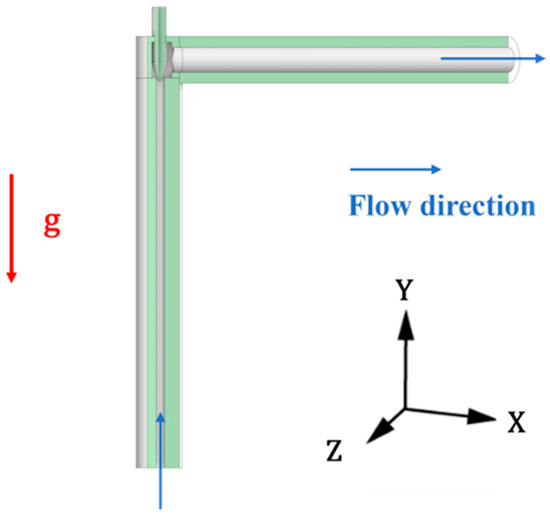
Figure 1.
Needle throttle valve upright placement model.
- 2.
- Needle throttle valve horizontal placement model
As shown in Figure 2, gravity in the horizontal placement model of the NTV follows the negative direction of the Z-axis, and the gas–solid two-phase flow enters the internal flow field of the NTV from the positive direction of the Y-axis. Compared with vertical and inverted placement, the gravity field is perpendicular to the flow direction of the gas–solid phase flow in the whole basin.
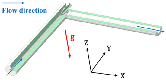
Figure 2.
Needle throttle valve horizontal placement model.
- 3.
- Needle throttle valve inverted placement model
As shown in Figure 3, in the NTV inverted placement model, the direction of gravity coincides with the flow direction when the gas–solid two-phase flow enters the upstream pipeline. When the gas–solid flow enters the downstream, the flow direction is perpendicular to the direction of gravity, which is the same as vertical placement.
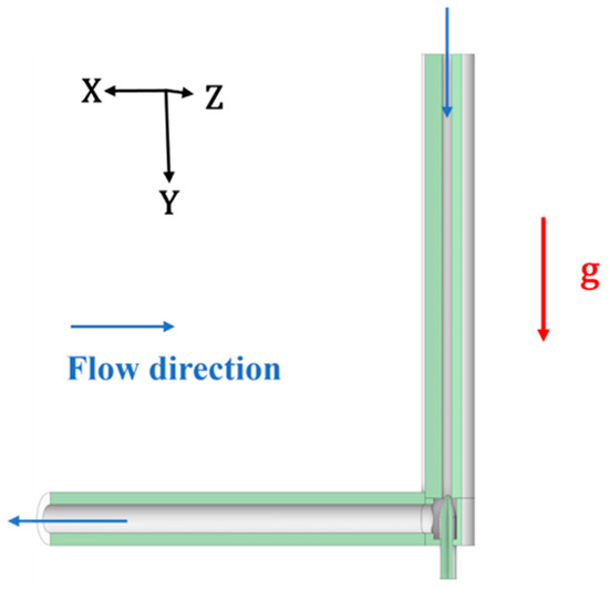
Figure 3.
Needle throttle valve inverted placement model.
After the gas produced from the wellhead of the shale gas field carrying solid particles enters the upstream pipeline section from the inlet, it first moves along the upstream pipeline to the valve chamber. Then, the gas flow and particles form a high-speed flow under the throttling action of the spool and then enter the valve chamber. Finally, the fully developed gas flow and undeposited particles in the valve chamber enter the downstream pipe. To avoid backflow, the length of the upstream and downstream pipelines was extended to more than 13 times the diameter of the pipe by referring to the valve flow test experiment proposed by the ISO (International Organization for Standardization) of the valve [19]. The key physical parameters of the model are shown in Table 1.

Table 1.
The main parameters of NTV and gas–solid two-phase flow.
3. Methodology
In order to improve the calculation accuracy, a ‘four-way’ coupled calculation model based on the CFD-DEM method is constructed. The interaction between the continuous phase (fluid) and the discrete phase (particles) is a two-way coupled interaction. In the calculation, the CFD calculation unit is responsible for calculating the continuous-phase fluid, the DEM calculation unit is responsible for the calculation of discrete-phase particles, and the two calculation units interact with each other through a coupling interface. The CFD solver used in this article is Fluent, and the DEM solver used in this article is EDEM. Considering the requirements of model characteristics and Rayleigh time, the time step in the DEM is set to 5 × 10⁻⁸ s, and time step in the CFD is set to 10−4 s. The flow time calculated for each example is 1.2 s. Within the first 0.2 s, the flow field in the valve gradually transitions from the unsteady state to the semi-steady state. The data from 0.2 s to 1.2 s are recorded for analysis.
3.1. Gas Phase Model
In fluid dynamics, matter is interrelated, and although the development of fluids is ever-changing, the mass continuity equation and the motion momentum equation summarized through a large number of experiments invisibly restrict the motion of fluids. Since the main goal of the calculation in this paper is the motion of fluids and particles, and it does not involve heat transfer and phase transition, the fluid-governing equations in this paper are mainly the continuity equation and the momentum equation.
Although mass and energy can be converted into each other when the speed of an object is close to the speed of light, when the speed of the object is much less than the speed of light, we can assume that the total mass of matter is constant, regardless of the form of change (physical or chemical) underway. As shown in Equation (1), the change in the mass of the mass conservation equation is 0.
where and are density and the time-averaged velocity of the nature gas, respectively. The boundaries can be classified into three types: a solid wall boundary, an inlet boundary, and an outlet boundary.
Equation (2) is the continuous-phase momentum conservation equation:
where is the pressure, and is the stress tensor. The boundaries can be divided into solid wall boundaries and symmetric boundaries.
Due to the very high Reynolds number in the pneumatic conveying equipment during shale gas extraction, the turbulence effect cannot be ignored. In this paper, we chose the SST turbulence model for the CFD simulations. It has very good applicability, accuracy, and reliability in predicting the phenomenon of wall flow separation, and it has been applied by a large number of scholars for the calculation of gate valves, butterfly valves, and other systems that are prone to strong flow separation [20]. The incompressible SST model for a single fluid is a two-way model with expressions (3) and (4).
The turbulence kinetic energy is
The specific dissipation rate is
Equation (5) is the expression for the generating term of turbulent energy:
Equation (6) is the expression for the blending function:
Equation (7) is the expression for the turbulent viscosity:
where is the turbulence kinetic energy; is the specific dissipation rate; is the magnitude of the shear strain rate; and are the turbulent Prandtl numbers for and ; ; ; and and are the blending functions.
3.2. Particle Motion Model
In this paper, the calculation of the motion of the discrete-phase particles is obtained by solving the differential equation of the momentum of the particles. By integrating the above differential equations, the motion parameters of each particle in the Lagrangian coordinate system of the flow field can be obtained. Although the change in particle shape will lead to a change in the particle shape coefficient, the main goal of this study is the effect of different particle diameters, VODs (valve opening degrees, which are the main way of adjusting the throttling effect of the valve), and placements on the erosion results. Therefore, the shape factor of the particles is omitted. In DEM, particles of different shapes are shaped mainly by the ‘cementation model’ of spherical particles (i.e., through a combination of multiple spherical particles). In the future, our team will use this model to study the erosion and crushing of particles of different shapes.
As shown in Equation (8), the law of conservation of momentum is actually Newton’s second law, the core principle of which is that the rate of change of fluid momentum is equal to the sum of the mass and surface forces acting on that volume. The motion of particles in the gas flow field can be divided into two categories—translational and rotational [3,13]. Equation (8) is the translational equation of particles.
where , and are the mass, velocity, and density of solid particles, respectively. and are the velocity and density of the gas flow phase, respectively. is the net external force experienced by the particle, including drag force pressure gradient force, contact force, Saffman lift, etc. [21,22].
Equation (9) is the rotation equation of particles.
where is the moment of inertia of the particle (referring to the moment of inertia of the sphere); is the angular velocity of the particles; is the tangential torque of the particle; is the rolling resistance torque of the particle, which has a counteracting effect on the self-rotation of the particle.
3.3. The Forces Acting on the Particles
As shown in Equation (8), the right side contains two terms, which are gravity and net external force. The net external forces on the particles in motion and the models used are further analyzed here.
- Drag force
Drag force, also known as drag, is the force generated by the relative motion of a continuous-phase fluid and a discrete-phase particle in the opposite direction of their respective motions [23]. It is one of the main forces affecting the movement of particles [24,25,26]. The drag force in this paper is calculated using Equation (10).
where is the mass of a single solid particle; is the velocity of the gas flow phase; is the velocity of the particles; and is the relaxation time, which is the time constant of the exponential decay of particle velocity due to drag [27]. The expression of is shown in Equation (11):
where is the density of the particle; is the particle diameter of the solid particle; is the molar viscosity of the gas flow; and and are the drag coefficient and relative Reynolds number of spherical solid particles, respectively [28].
Here, we write the drag Equation (10) as an equation related to , , and in order to understand its relationship to the individual variables in more depth:
As shown in Equation (13), the Stokes number (Stk.) is a dimensionless number. The Stk. is mainly used to describe the motion behavior of suspended particles in a fluid. It can help us to better understand the force of the gas flow on the solid particles.
where is the velocity of the gas flow away from the obstacle; is the characteristic dimension of the obstacle or the characteristic length in the flow [29]; and is the relaxation time of the particles [30]. When the Stk. of the particle is smaller (Stk. ), it is easier for the particle to follow the streamlines of the gas flow and to achieve ‘perfect advection’, while when the particle diameter is larger, its Stk. is also larger (Stk. ), and inertia and gravity will dominate its trajectory more [31]. In the subsequent research, we will introduce particles of different sizes in the same case to explore the influence of collisions between particles of different sizes on the particle distribution.
- 2.
- Particle–particle interaction forces
One of the biggest advantages of the CFD-DEM method over other models is that it is a four-way coupled calculation model that takes the interaction forces between particles into account. In this paper, the Hertz–Mindlin (no-slip) contact model is used to calculate the contact force between particles. The main forces in the particle contact model are the normal force (), tangential force (), and their corresponding normal damping force () and tangential damping forces ().
Equation (14) is the normal force .
where is the normal overlap (as shown in Figure 4), and and are the equivalent Young’s modulus and radius, respectively.
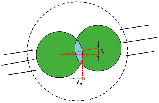
Figure 4.
Schematic diagram of particle contact.
Equation (15) is the normal damping force
where e is the coefficient of restitution, is the normal stiffness, is the equivalent mass, and is the normal component of the relative velocity.
Equation (16) is the normal force .
where is the tangential overlap (as shown in Figure 4), and is the tangential stiffness.
Equation (17) is the tangential damping force .
where is the relative tangential velocity.
- 3.
- Interaction forces between the particle and wall
In the CFD-DEM model, the contact between the particle and the wall is calculated by treating the wall as particles with an infinite radius.
- 4.
- Saffman lift
When a particle is in a flow field with a velocity gradient, it is subject to lateral lift even if the particle does not rotate itself, and the trajectory of the particle changes under the influence of this force, as shown in Figure 5. Since the velocity gradient near the wall is often large, and the problem studied in this paper is mainly the erosion of the wall, this force is also considered in the external force. The expression for the Saffman lift is shown in Equation (18).
where ; is the deformation tensor; and is the dynamic viscosity [32,33].
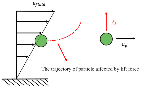
Figure 5.
Schematic diagram of the effect of Saffman lift on particle motion.
3.4. Particle Erosion Model
The main objective of this paper is to study the erosion of the inner wall surface of the valve by solid particles carried in the gas extracted from the wellhead. Compared with other erosion models, the OKA erosion model is the most advantageous for integrating the properties of solid particles (velocity, mass, diameter) and the erosion surface of the valve (density, hardness, curvature) [34,35]. Although the E/CRC model can also consider the surface shape of the structure, it lacks in terms of particle geometry. Using the OKA model, the physical properties of the particles and the characteristics of the complex surfaces of the valve interior can be fully considered.
Therefore, the OKA erosion model, as first proposed by Oka and Yoshida [36,37], is used in this chapter as a computational model for the erosion of the inner surface of the valve. As shown in Equation (19), there are two input parameters in the OKA erosion model, which are the Vickers hardness () and the material wear constant ().
where is the surface erosion depth; is the impact velocity; is the wear constant; is the particle diameter; is the particle mass; is the particle projection area; is a coefficient derived from the experiments; and () is the impact angle of the particles. The values of the above parameters are given in Table 2. In addition, is a function of the impact angle of the particle, and its expression is given in Equation (20).
Table 2.
The constant values of the OKA erosion model.
4. Validation
4.1. Mesh Independence
In this paper, the finite volume method is used to solve the fluid computational domain, which is divided into meshes of different volumes. The finite volume method solves conserved quantities in integral form by discretizing the governing equations, and the results are directly influenced by meshing. In complex geometric structures such as NTV, rough or poorly aligned meshes can lead to significant numerical diffusion and truncation errors, resulting in inaccurate prediction of sharp gradients in velocity and pressure fields. The finer the mesh, the smaller the discrete error, but the more the computational resources are required [38]. Mesh independence validation is the bridge between ‘numerical discretization’ and ‘physical reality’. It strikes a balance between computational accuracy and computational efficiency by comparing solutions from multiple sets of grids and confirming whether the results converge to a continuous solution. Due to the very drastic changes in the flow field in the throttle channel as well as in the valve chamber, we locally refine the mesh in this region. Figure 6 is the schematic diagram of the meshing of NTV.
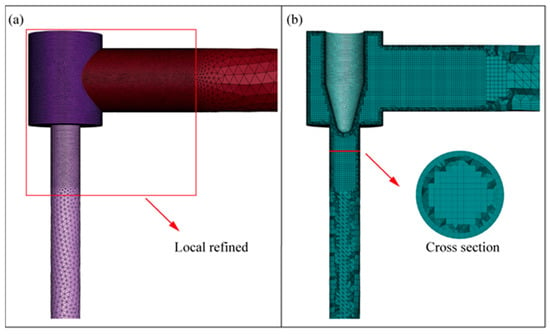
Figure 6.
Schematic diagram of the (a) surface mesh (b) volume mesh.
As shown in Table 3, the mesh of the NTV is divided into M1-M4 levels. The number of meshes is mainly controlled by controlling the local refinement size, the surface mesh size, and the volume mesh size. Table 4 shows the quality parameters corresponding to the four levels of mesh, indicating that the quality of the four levels of grids can meet the requirements for calculation.
Table 3.
The quantity of mesh under different levels.
Table 4.
Mesh quality parameters.
Since the main research goal of this paper is to assess the erosion of valves, the erosion rate of valves is selected as the parameter for the validation of mesh independence.
Figure 7 shows the results of the valve mesh independence validation. The abscissa is the level of the mesh, and it can be seen from Table 3 that the number of meshes increases gradually from M1 to M4. The ordinate is the value of the erosion rate. It can be found that with the increase in the level, the calculation results of the maximum erosion rate gradually converge to the calculated value of the M4 level. When the level reaches M3, the error from the value of M4 is less than 2%. At this point, the increase in the number of meshes has a very weak effect on reducing the discrete error. This also shows that the M3 mesh can be used to balance the calculation accuracy and efficiency. Therefore, in this paper, the M3 level mesh is selected for calculation.
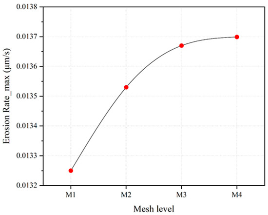
Figure 7.
Mesh independence validation.
4.2. Flow Erosion Accuracy Validation
Verifying the computational accuracy of the model before the computation starts can help to improve the credibility of the model. In this paper, the physical and mathematical models of the vertical placement method were validated using the experimental results of valve erosion by H. Zhu et al. [39]. Figure 8 shows the control results of the experiment and simulation during the validation process, mainly by comparing the experimental measurements of the erosion rate of different positions of the valve with the simulated values.
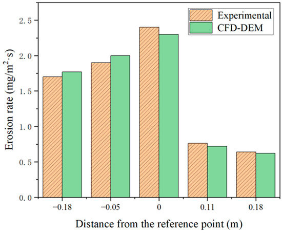
Figure 8.
Comparison of CFD and experimental results.
As can be seen from Figure 8, the CFD-DEM erosion model of the NTV in this paper not only has a small error (the average relative error is less than 10%) when compared with the experimental results; it also has a high degree of agreement in terms of the trends in changes. Therefore, it can be considered that the physical and mathematical models constructed in this paper are accurate and reliable. In the future, our team will adopt more advanced equipment in the early experimental stage and collect more experimental data, striving to make greater progress in research on valve gas–solid two-phase flow.
5. Result and Discussion
In this section, firstly, the distribution characteristics of the gas flow field inside the NTV are analyzed in the absence of particles; then, the distribution characteristics of particles in three different placements and using different VODs (valve opening degrees, which are the main way of adjusting the throttling effect of the valve) are investigated; finally, the erosion rates of the various parts of the valve when using different VODs as well as particle diameters are investigated.
5.1. Pure Gas Flow Field in the Valve
The first factor to be analyzed is the distribution characteristics of the pure gas flow field, for which only the CFD method is used for the calculation of the gas-phase flow. As shown in Figure 9, after the gas flow enters the upstream pipe from the inlet, it first enters the valve chamber under the throttling action of the spool, and the gas flow is accelerated as it passes through the throttling channel. With the increase in the VOD, the throttling effect of the needle throttle valve gradually weakens, and the most extreme velocity value in the flow field also decreases gradually. It is worth noting that there is a low-speed zone at the apex of the spool.
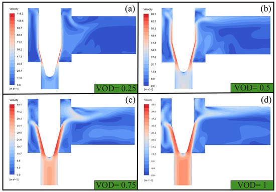
Figure 9.
Gas flow field when using different valve opening degrees (VODs) (a) VOD = 0.25 (b) VOD = 0.5 (c) VOD = 0.75 (d) VOD = 1.
5.2. Effect of Different Placement Methods on Particle Motion
As previously mentioned, the main forces that the particles are subjected to during the whole process of movement are inertial force, trailing force, gravity, and so on. In models with different placement methods, the transformation timing and magnitude of kinetic energy and gravitational potential energy of solid particles undergo significant changes due to variations in the gravitational field. These changes profoundly affect particle motion and consequently influence particle deposition and valve erosion. Figure 10 illustrates the distribution and deposition of particles with a diameter of 400 μm in an NTV under different VODs and placement methods.
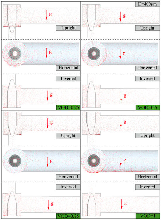
Figure 10.
Particle distribution with different valve openings and placements (the particle diameter is 400 μm).
In terms of the horizontal placement method, when the VODs are 0.25 and 1, there is obvious deposition; the difference is that when the VOD is 0.25, the deposition of particles is mainly concentrated in the lower part of the chamber. When the VOD is 1, the deposition of particles is more serious, not only in the lower part of the chamber but also in the upstream pipeline and downstream of the more obvious deposition. When the VOD is 0.5 and 0.75, the deposition phenomenon is significantly reduced. This is because when the VOD is 0.25, the collisions between particles and particles and the inner wall of the valve in the chamber are very violent, and these collisions will lead to a large amount of kinetic energy being lost from particles and deposited in the chamber. When the valve is fully open, the velocity of the valve gas flow field decreases dramatically, which leads to a significant reduction in the kinetic energy enhancement of the particles by the drag force. This results in significant deposition of particles occurring throughout the basin.
In the case of the inverted placement, the particle distribution is more homogeneous. Unlike the vertical placement, the particle deposition is concentrated in the left chamber of the valve.
Figure 11 shows the particle distribution and deposition of different VODs and placement methods when the particle diameter is 600 μm. As the particle diameter increases, the Stokes number (Stk.) of the particles and the magnitude of the gravity force on the particles also increase gradually. It can be found that with the increase in particle diameter, the particle deposition phenomenon of a smaller VOD is obviously aggravated, while the particle deposition phenomenon is greatly improved when the valve is fully open. This is because as the particle diameter increases, the kinetic energy lost by particle collision gradually increases. At the same time, the effect of drag force applied to the particles by the gas flow on particle movement gradually weakens. After the collision has occurred, the particles do not receive enough kinetic energy to replenish and thus are deposited in the valve.
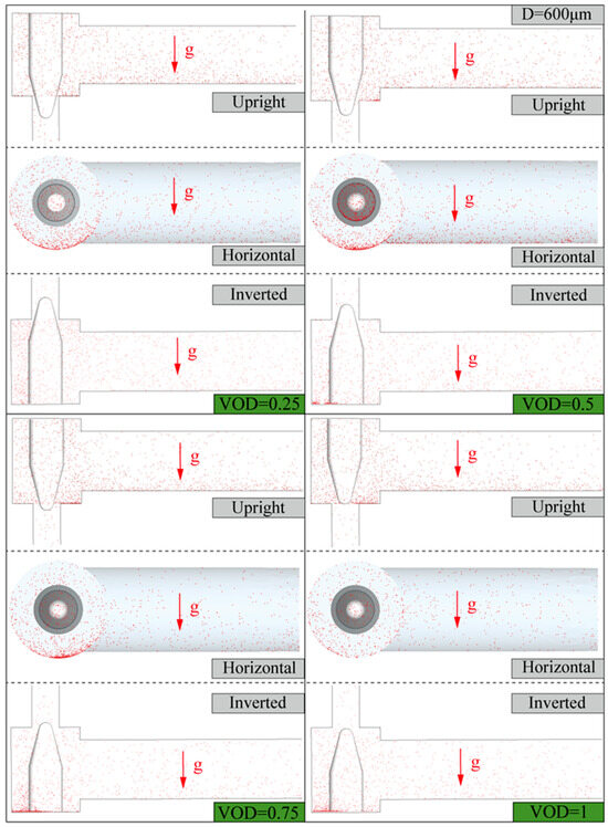
Figure 11.
Particle distribution with different valve openings and placements (the particle diameter is 600 μm).
Figure 10 and Figure 11 show that in the inverted placement method, the deposition of particles is aggravated with the increase in particle diameter when using different VODs. When utilizing the horizontal placement method, the deposition of particles is greatly affected by both the VODs and particle diameters. In addition, the deposition of particles in the upstream pipeline in the horizontal placement method is not negligible compared to the other two placement methods.
5.3. Effect of Different Placement on Valve Erosion
In all three placement methods, particles not only deposit and block flow channels in upstream, chambers, and downstream; they also continuously collide with the inner walls of the valve, leading to mass loss in pipeline components and eventual valve failure. This section investigates the impact of placement methods on valve erosion by analyzing the average and maximum erosion rates of the valve.
5.3.1. Average Erosion Rate of Valve Components
The average erosion rate is described as the total erosion volume of a component divided by its surface area, reflecting the overall erosion status of valve components. This metric effectively highlights the influence of placement methods on particle motion. In this section, the average erosion rate of four different components of NTV is studied for both a small valve opening degree (VOD = 0.25) and a large valve opening degree (VOD = 1). Figure 12, Figure 13, Figure 14 and Figure 15 present the average erosion rates of the spool, chamber, upstream, and downstream, respectively.
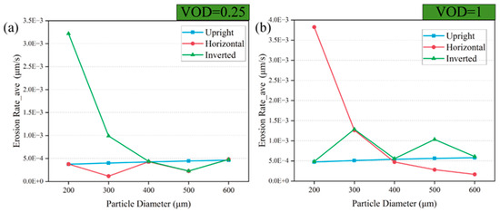
Figure 12.
Average erosion rate of the spool when using small and large VODs (a) VOD = 0.25 (b) VOD = 1.
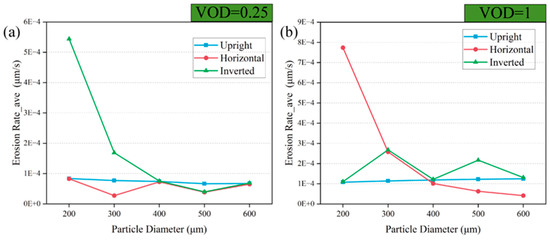
Figure 13.
Average erosion rate of the chamber when using small and large VODs (a) VOD = 0.25 (b) VOD = 1.
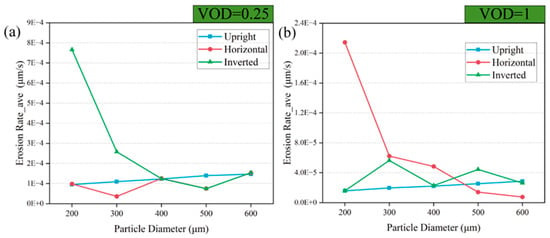
Figure 14.
Average erosion rate of the upstream when using small and large VODs (a) VOD = 0.25 (b) VOD = 1.
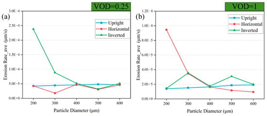
Figure 15.
Average erosion rate of the downstream when using small and large VODs (a) VOD = 0.25 (b) VOD = 1.
It can be seen from Figure 12 that when the VOD is small, the inverted placement of the NTV is severely eroded when there is a small particle diameter. When the valve is fully open, the NTV placed horizontally is also severely eroded under small-particle-diameter conditions. When the NTV is placed in an inverted placement, the direction of gravity is first consistent with the direction of particle movement. When the particle diameter is small, under the double influence of gravity and drag force, the kinetic energy of the particles in the collision with the spool is greater, which is also the reason for the higher erosion rate. When the NTV is placed horizontally, because the direction of gravity and the direction of gas–solid two-phase flow is perpendicular to the direction of movement, when the particle diameter is large and the throttle channel area is large, most of the particles will deviate from the spool trajectory. This also explains the phenomenon that the erosion rate of the spool decreases with increasing particle diameter when the valve is placed horizontally in Figure 12b. Figure 13, Figure 14 and Figure 15 show almost the same pattern as Figure 12, which suggest that there may be a ‘bias wear’ phenomenon in the valve when it is placed horizontally.
5.3.2. Maximum Erosion Rate of the Spool
Due to the unique physical structure of the NTV, localized excessive erosion can directly cause valve failure, posing significant safety risks in shale gas field operations. As indicated in earlier findings, the spool is the most erosion-prone component.
Building on the analysis of average erosion rates, this section investigates the maximum erosion rate (set to the erosion rate at the most severely eroded location) of the spool under different placement methods. Figure 16 illustrates the maximum erosion rates of the spool when using three placement methods and various VODs and particle diameters.
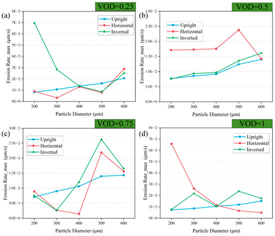
Figure 16.
Maximum erosion rate of the spool at Different VODs (a) VOD = 0.25 (b) VOD = 0.5 (c) VOD = 0.75 (d) VOD = 1.
When the VOD = 0.25 and 1, the maximum erosion rate of the spool when using the three types of placement exhibits a similar pattern of change to the average erosion rate in Section 5.3.1. When the VOD is 0.5, the particle diameter gradually increases from 200 μm to 500 μm; the erosion rate of the spool placed uprightly, horizontally and inverted gradually increases, among which the erosion rate of the spool placed horizontally is greater than that of the other two placements. When the particle diameter increases from 500 μm to 600 μm, the erosion rate of the spool continues to increase with the inverted and horizontal placement, but the erosion rate of the spool in the horizontal placement decreases steeply.
When the VOD is 0.75, the maximum erosion rate of the spool fluctuates greatly under horizontal and inverted placement modes. Specifically, the erosion rate of the spool is approximately in three placement modes when the particle diameter is 200 μm and 600 μm. As the particle diameter increases, the erosion rate of the spool in horizontal and inverted placement decreases first and then increases.
Figure 17 shows contour plots of the erosion of the spool of the NTV with a 0.25 degree of opening and at full opening when placed horizontally. In this figure, the redder the color, the more significant the erosion. It can be clearly observed that there is a serious ‘bias wear’ phenomenon in the spool. Regardless of the VOD and particle diameter, the growth of the ‘bias wear’ is at the lower edge of the spool, which corresponds to the shrinkage of the erosion area at the upper edge of the spool. Although the erosion rate of the valve can be divided into the average erosion rate and maximum erosion rate, excessive local erosion can have a serious impact on the air tightness of the valve. The spool is one of the most critical components of the valve airtightness, and when the valve is installed horizontally or at an angle, the service time of the valve is shortened. In addition, due to the ‘shift’ in the position of the erosion propagation, the annular edge of the spool should be inspected when checking for erosion, avoiding only the local position.
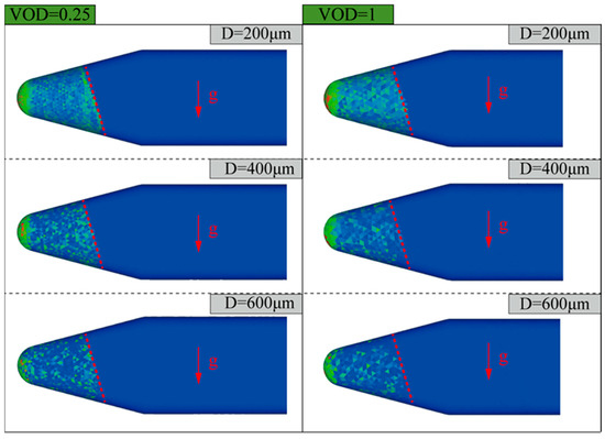
Figure 17.
Spool erosion contours when using small and large VODs.
5.4. Discussion
At present, the main method of erosion simulation is CFD-DPM. Although it can be carried out with high efficiency, it is less accurate when assessing high particle density due to the ignorance of the interaction between particles. In this paper, a gas–solid two-phase flow erosion model of NTV is constructed based on the CFD-DEM method. Compared with similar studies, this paper not only adopts a ‘four-way’ coupling method with higher accuracy but also considers the influence of on-site valve installation on erosion. Our research finds that the spool is the area of the valve that is most severely eroded, and when placed horizontally, it exhibits a serious ‘bias wear’ phenomenon. The research results herein can provide references for the design optimization and on-site maintenance of valve performance.
Although this paper discovers some laws of valve erosion, there are some shortcomings. First, this paper ignores the shape factors of particles and uses a soft sphere model for calculation, which may have a certain impact on the accuracy of calculations. In addition, although this paper uses certain experimental data to verify the calculation accuracy of the simulation, the sampling point density of the experiment is not high, making it difficult to verify the erosion results at each location.
In the future, our team will adopt more advanced equipment in the early experimental stage and collect more experimental data to establish an erosion sample database, in doing so striving to make greater progress in research on valve gas–solid two-phase flow.
6. Conclusions
Based on the ‘four-way’ coupled calculation model of CFD-DEM, this paper studies the influences of particle diameter, placement method, and VOD on the erosion effect and draws the following conclusions.
- When placed in reverse, particle deposition at different points intensifies with the increase in particle diameter. When placed horizontally, particle deposition is greatly affected by VOD and particle diameter. Furthermore, in the horizontally placed model, the deposition of particles in the upstream pipeline also cannot be ignored.
- When placed horizontally, the spool is subjected to a severe ‘bias wear’ phenomenon, which grows along the lower edge of the spool, regardless of the VOD and particle diameter. Correspondingly, the erosion area along the upper edge of the spool shrinks. The scope of the ‘bias wear’ area is almost independent of the VOD and particle diameter.
Author Contributions
Conceptualization, Z.W., Y.L., M.L., F.W., Y.W., S.D., W.W. and B.H.; methodology, Z.W., Y.L., M.L., S.D., W.W. and B.H.; software, Z.W., F.W. and S.D.; validation, Z.W., M.L., F.W., and Y.W.; formal analysis, Y.L., M.L., F.W., Y.W. and S.D.; investigation, Z.W., Y.L., M.L., F.W., S.D., W.W. and B.H.; resources, F.W., Y.W. and W.W.; data curation, Y.L., F.W., Y.W. and S.D.; writing—original draft preparation, Z.W., Y.L., M.L. and B.H.; writing—review and editing, Z.W., Y.L., M.L., F.W., S.D. and B.H.; visualization, W.W. and S.D.; supervision, B.H.; project administration, B.H.; funding acquisition, B.H. All authors have read and agreed to the published version of the manuscript.
Funding
This study was supported by the financial support of the Natural Science Foundation of Chongqing Municipality (CSTB2023NSCQ-MSX0050), the Zhejiang New Talent Plan of Student’s Technology and Innovation program (No. 2024R411B040), the Project of Sinopec Sales Co., LTD. (32850024-23-ZC0607-0001), and the Science and Technology Project of Daishan County, Zhoushan City (202215).
Data Availability Statement
Data are contained within the article.
Conflicts of Interest
Author Fubin Wang was employed by China petroleum pipeline engineering Co., Ltd. The remaining authors declare that the research was conducted in the absence of any commercial or financial relationships that could be construed as a potential conflict of interest.
Abbreviations
The following abbreviations are used in this manuscript:
| CFD | Computational fluid dynamics |
| DPM | Discrete phase method |
| DEM | Discrete element method |
| NTV | Needle throttle valve |
| VOD | Valve opening degree |
| ave | Average value |
| max | Maximum value |
| Particle diameter, (m) | |
| Equivalent Young’s modulus, (Pa) | |
| Vicker’s hardness, (GPa) | |
| Static pressure, (Pa) | |
| ) | |
| Stk. | Stokes number |
| ) | |
| ) |
References
- Zhang, Y.; Tian, B.; Xu, Z.; Chen, Q.; Xiao, Y.; Liu, Y.; Yang, Q.; Wang, L.; Huang, L.; Feng, X. Gas sorption in shale media by molecular simulation: Advances, challenges and perspectives. Chem. Eng. J. 2024, 487, 150742. [Google Scholar]
- Wang, J.; Wang, K.; Shan, X.; Taylor, K.G.; Ma, L. Potential for CO2 storage in shale basins in China. Int. J. Greenh. Gas Control 2024, 132, 104060. [Google Scholar] [CrossRef]
- Ye, J.; Cui, J.; Hua, Z.; Xie, J.; Peng, W.; Wang, W. Study on the high-pressure hydrogen gas flow characteristics of the needle valve with different spool shapes. Int. J. Hydrogen Energy 2023, 48, 11370–11381. [Google Scholar] [CrossRef]
- Yin, Q.; Zeng, B.; Zhao, J.; Ren, L.; Chen, X.; Lin, R.; Hu, Y.; Du, L.; Li, Z.; Hu, D.; et al. Ten years of gas shale fracturing in China: Review and prospect. Nat. Gas Ind. B 2022, 9, 158–175. [Google Scholar]
- Guo, J.; Lu, Q.; He, Y. Key issues and explorations in shale gas fracturing. Nat. Gas Ind. B 2023, 10, 183–197. [Google Scholar] [CrossRef]
- Wu, J.; Tan, D.; Yin, Z.; Tan, Y.; Li, Z.; Wang, T.; Li, L. Mass transfer mechanism of multiphase shear flows and interphase optimization solving method. Energy 2024, 292, 130475. [Google Scholar] [CrossRef]
- Liu, E.-B.; Huang, S.; Tian, D.-C.; Shi, L.-M.; Peng, S.-B.; Zheng, H. Experimental and numerical simulation study on the erosion behavior of the elbow of gathering pipeline in shale gas field. Pet. Sci. 2024, 21, 1257–1274. [Google Scholar] [CrossRef]
- Luo, P.; Jia, W.; Wang, Y.; Li, C.; Song, X.; Zhang, Y.; Hu, X. Experimental and numerical simulation of erosion-corrosion of 90 steel elbow in shale gas pipeline. J. Nat. Gas Sci. Eng. 2021, 89, 103871. [Google Scholar]
- Jia, M.; Wei, Y.; Yan, C.; Jiang, P.; Xu, R. Experimental study of gas-solid flow characteristics and flow-vibration coupling in a full loaded inclined pipe. Powder Technol. 2021, 384, 379–386. [Google Scholar] [CrossRef]
- Zhao, X.; Cao, X.; Xie, Z.; Cao, H.; Wu, C.; Bian, J. Numerical study on the particle erosion of elbows mounted in series in the gas-solid flow. J. Nat. Gas Sci. Eng. 2022, 99, 104423. [Google Scholar] [CrossRef]
- Li, Q.; Cao, X.; Xiong, N.; Karimi, S.; Xie, Z.; Darihaki, F.; Zhang, J. Effect of cell size on erosion representation and recommended practices in CFD. Powder Technol. 2021, 389, 522–535. [Google Scholar]
- Zhang, D.; Li, A.; Dou, X.; Li, Y.; Xiang, W.; Li, B.; Ju, M. CFD-DPM modelling of solid particle erosion on weld reinforcement height in liquid-solid high shear flows. Powder Technol. 2023, 427, 118773. [Google Scholar] [CrossRef]
- Li, R.; Sun, Z.; Li, A.; Li, Y.; Wang, Z. Design optimization of hemispherical protrusion for mitigating elbow erosion via CFD-DPM. Powder Technol. 2022, 398, 117128. [Google Scholar] [CrossRef]
- Wang, H.; Huang, F.; Fazli, M.; Kuang, S.; Yu, A. CFD-DEM investigation of centrifugal slurry pump with polydisperse particle feeds. Powder Technol. 2024, 447, 12020. [Google Scholar] [CrossRef]
- Li, Z.; Chen, H.; Wu, Y.; Xu, Z.; Shi, H.; Zhang, P. CFD-DEM analysis of hydraulic conveying of non-spherical particles through a vertical-bend-horizontal pipeline. Powder Technol. 2024, 434, 119361. [Google Scholar] [CrossRef]
- Xu, L.; Zhang, Q.; Zheng, J.; Zhao, Y. Numerical prediction of erosion in elbow based on CFD-DEM simulation. Powder Technol. 2016, 302, 236–246. [Google Scholar] [CrossRef]
- Lin, Z.; Sun, X.; Yu, T.; Zhang, Y.; Li, Y.; Zhu, Z. Gas–solid two-phase flow and erosion calculation of gate valve based on the CFD-DEM model. Powder Technol. 2020, 366, 395–407. [Google Scholar] [CrossRef]
- Lin, Z.; Zhang, Y.; Li, Y.; Li, X.; Zhu, Z. Prediction of particle distribution and particle impact erosion in inclined cavities. Powder Technol. 2017, 305, 562–571. [Google Scholar] [CrossRef]
- He, J.; Peng, W.; Liu, M.; Huang, X.; Han, S. The flow characteristics of gas–solid two-phase flow in an inclined pipe. Adv. Powder Technol. 2025, 36, 104725. [Google Scholar] [CrossRef]
- Menter, F.R. Two-equation eddy-viscosity turbulence models for engineering applications. AIAA J. 1994, 32, 1598–1605. [Google Scholar] [CrossRef]
- Chauhan, V.; Gudjonsdottir, M.; Saevarsdottir, G. Silica particle deposition in superheated steam in an annular flow: Computational modeling and experimental investigation. Geothermics 2020, 86, 101802. [Google Scholar] [CrossRef]
- Chang, T.-J.; Hu, T.-S. Transport mechanisms of airborne particulate matters in partitioned indoor environment. Build. Environ. 2008, 43, 886–895. [Google Scholar] [CrossRef]
- Wen, C.Y. Mechanics of fluidization. Fluid Part. Technol. Chem. Eng. Progress. Symp. Ser. 1966, 62, 100–111. [Google Scholar]
- Wang, K.; Li, X.; Wang, Y.; He, R. Numerical investigation of the erosion behavior in elbows of petroleum pipelines. Powder Technol. 2017, 314, 490–499. [Google Scholar] [CrossRef]
- Habib, M.; Badr, H.; Ben-Mansour, R.; Said, S. Numerical calculations of erosion in an abrupt pipe contraction of different contraction ratios. Int. J. Numer. Methods Fluids 2004, 46, 19–35. [Google Scholar] [CrossRef]
- Michaelides, E.E.; Sommerfeld, M.; van Wachem, B. Multiphase Flows with Droplets and Particles; CRC Press: Boca Raton, FL, USA, 2022. [Google Scholar]
- Gosman, A.; Loannides, E. Aspects of computer simulation of liquid-fueled combustors. J. Energy 1983, 7, 482–490. [Google Scholar] [CrossRef]
- Morsi, S.; Alexander, A. An investigation of particle trajectories in two-phase flow systems. J. Fluid Mech. 1972, 55, 193–208. [Google Scholar] [CrossRef]
- Willert, C.; Wereley, S.T.; Kompenhans, J. Particle Image Velocimetry, 3rd ed.; Springer International Publishing: Berlin/Heidelberg, Germany, 2018. [Google Scholar]
- Kolev, N.I.; Kolev, N.I. Multiphase Flow Dynamics: Fundamentals; Springer: Berlin/Heidelberg, Germany, 2005. [Google Scholar]
- Tropea, C.; Yarin, A.L.; Foss, J.F. Springer Handbook of Experimental Fluid Mechanics; Springer: Berlin/Heidelberg, Germany, 2007. [Google Scholar]
- Li, A.; Ahmadi, G. Dispersion and deposition of spherical particles from point sources in a turbulent channel flow. Aerosol Sci. Technol. 1992, 16, 209–226. [Google Scholar] [CrossRef]
- Saffman, P.G. The lift on a small sphere in a slow shear flow. J. Fluid Mech. 1965, 22, 385–400. [Google Scholar] [CrossRef]
- Deng, L.; Zhang, K.; Chen, Y.; Ni, H. Numerical simulation study on the erosion and wear of galvanized coatings on steel structures under the action of wind and sand. J. Phys. Conf. Ser. 2023, 2566, 012037. [Google Scholar] [CrossRef]
- Amadi, A.H.; Mohyaldinn, M.; Abduljabbar, A.; Ridha, S.; Avilala, P.; Owolabi, G.T. Wear analysis of NiTi sand screens using Altair discrete element method. Materials 2024, 17, 281. [Google Scholar] [CrossRef] [PubMed]
- Oka, Y.; Yoshida, T. Practical estimation of erosion damage caused by solid particle impact: Part 2: Mechanical properties of materials directly associated with erosion damage. Wear 2005, 259, 102–109. [Google Scholar] [CrossRef]
- Oka, Y.I.; Okamura, K.; Yoshida, T. Practical estimation of erosion damage caused by solid particle impact: Part 1: Effects of impact parameters on a predictive equation. Wear 2005, 259, 95–101. [Google Scholar] [CrossRef]
- Wu, Z.; Wang, C.; Lang, R.; Li, Y.; Hong, B. The distribution of components in hydrogen-blended pipelines under different gas stream injection pattern. Fuel 2024, 375, 132577. [Google Scholar] [CrossRef]
- Zhu, H.; Pan, Q.; Zhang, W.; Feng, G.; Li, X. CFD simulations of flow erosion and flow-induced deformation of needle valve: Effects of operation, structure and fluid parameters. Nucl. Eng. Des. 2014, 273, 396–411. [Google Scholar] [CrossRef]
Disclaimer/Publisher’s Note: The statements, opinions and data contained in all publications are solely those of the individual author(s) and contributor(s) and not of MDPI and/or the editor(s). MDPI and/or the editor(s) disclaim responsibility for any injury to people or property resulting from any ideas, methods, instructions or products referred to in the content. |
© 2025 by the authors. Licensee MDPI, Basel, Switzerland. This article is an open access article distributed under the terms and conditions of the Creative Commons Attribution (CC BY) license (https://creativecommons.org/licenses/by/4.0/).