Abstract
In the context of accelerated digitization and the transition to sustainability, this study explores the relationship between the use of cloud computing services and greenhouse gas (GHG) emissions in the IT and communications sectors at the European level using panel data provided by Eurostat for the period 2014–2021. The initial set included 14 countries, but due to incomplete data, the final analysis was performed on a consistent and complete dataset comprising 8 countries: Bulgaria, Cyprus, Denmark, Hungary, Latvia, Norway, Poland, and Romania. The applied methodology includes VAR and VECM econometric models, the Granger causality test, impulse response functions, and variance decomposition. The results show a long-term cointegrating relationship between the variables, highlighting the existence of mass and energy transfer to centralized infrastructures such as data centers. The IT subsectors (J62_J63) demonstrate superior efficiency in reducing GHG emissions compared to the general communications sector (J), highlighting the positive impact of a high level of digitization. Although the research provides valuable insights into the relationship between digitization and sustainability, a major limitation is that not all EU countries are represented. This study provides actionable policy recommendations to minimize the ecological impact of digital technologies and enhance resource efficiency in the green transition era.
1. Introduction
The soaring trend of cloud computing has changed the information technology and communications industries and how data are stored, processed, and transmitted. Between 2014 and 2021, virtualization, growth in internet penetration, and demand for geographically is distributed, scalable, and cost-effective. IT infrastructure drove the transition from on-premises service delivery to cloud services. Cloud computing has revolutionized resource utilization, enhancing efficiency and accelerating digital transformation across industries. Despite these advancements, concerns about its environmental sustainability persist. Mass and energy flows linked to data centers and associated GHG emissions raise questions about whether digitalization can align with green transition goals. To address these concerns, this study employs econometric methods to analyze the relationship between cloud computing adoption (measured through E_CC) and GHG emissions, offering insights into the role of digitalization in fostering sustainability. Mass and energy flows refer to cloud computing infrastructure’s physical resource transfers and energy consumption processes [1].
The advent of cloud computing is changing how businesses operate and the IT and communications arenas, offering unheard-of levels of efficiency, innovation, and scalability. In the last few years, however, huge attention has been paid to the environmental implications of this technological transformation. Cloud services have transformed mass and energy flows in global data centers, significantly impacting resource consumption and GHG emissions. Although cloud computing could potentially yield environmental advantages, such as lowering the costs of on-premises infrastructure and optimizing energy use, it also entails risks related to the sustainability of energy use in large-scale data centers and the energy footprint of support infrastructure [2].
Cloud computing operates via data centers where computing resources are combined and processed as required; however, it is on demand. This centralization can increase efficiency, but it also centralizes energy use and consumption, thereby increasing the environmental footprint of cloud services [3]. At the heart of this discourse lies a dual challenge: how the cloud ecosystem impacts mass and energy flows and quantifies resulting environmental impacts, particularly in setting Europe’s ambitious climate targets [4,5].
For example, Europe is always extremely vanguard regarding sustainability initiatives in search of convergence between technological progress and environmental preservation. As one of the world’s largest cloud users, the European Union (EU) has been challenged to align its commitment to cut GHG emissions by 55% by 2030, as defined in the European Green Deal, with the fast-growing adoption of IT services. This analysis of how the growth of IT and communications sector cloud computing has influenced the broader energy ecosystem and emitted from 2014 to 2021 (except 2019) is a critical juncture.
This seven-year study looks at how cloud computing adoption in Europe fits in with the environmental implications of technological innovation and how technological innovation is related to energy efficiency and sustainability. This paper looks at trends in energy consumption, data center efficiency, and emissions profiles in order to provide a complete picture of how cloud computing is influencing mass as well as energy flows and the wider environmental targets that Europe has set out. Furthermore, the analysis also reveals what IT and communications sectors have done to reduce their ecological footprint, where integrating renewable energy, developing more efficient cooling technologies, and transitioning to more energy-efficient architectures are trends [6,7].
Cloud technology has driven the IT sector to a growing share of global electricity consumption and carbon emissions, motivating researchers and policy makers to assess its broader ecological impacts. Some of the environmental challenges associated with data center utilization can be mitigated through studies that show the ability to optimize data center operations, transition to renewable energy sources, and implement energy-efficient technologies [8,9]. Addressing the complex nexus of cloud computing and mass and energy flows, as well as greenhouse gas emissions, this article considers technological progress and sustainability objectives.
2. Scientific Background
2.1. Cloud Computing Adoption
Cloud computing has developed into a rapidly evolving tool for businesses and individuals to access and use computational resources. Virtualization, scalable infrastructure, and internet connectivity are essential for delivering on-demand computing resources in cloud computing. Its technological and economic benefits have been widely acknowledged, but its environmental implications, particularly those related to mass and energy flows, have become an area of intense academic and industrial research. This chapter analyzes the literature surrounding the dynamic nature of cloud computing’s energy consumption, GHG emissions, resource usage, and mitigation strategies.
Cloud computing became a revolution in the mid-2000s, bringing infrastructure, platforms, and software as a service into its basket [10]. Marston et al. [11] reveal that cloud services have been motivated to meet growing business needs for flexible, inexpensive, and efficient IT solutions [12]. Other significant advances, for instance, in server virtualization or containerization, alongside software-defined networking, are also significant pillars supporting cloud solutions [13,14].
The usage of cloud services in Europe from 2014 to 2021 has increased due to digital business strategies and the European agenda for a digital future [15,16]. During this period, the derived facilities included hyperscale data network centers and edge computing facilities in response to gargantuan data processing and localized, low-latency applications. According to Marston et al. [11], this growth has changed the IT environment anew, opening fresh opportunities for creative endeavors and raising fresh obstacles in environmental management. He highlights the contribution of cloud computing to reducing operational costs and resource consumption by IT infrastructure consolidation [11,17]. At the same time, Horner et al. [18] point out that the adoption of cloud computing contributes to decreasing local energy consumption but may increase the global demand for electricity for data centers.
Cloud computing has been widely recognized as a driver of digital transformation, offering substantial benefits such as cost reduction, scalability, and energy efficiency [19,20,21]. Energy efficiency generated by cloud computing comes from various hardware solutions and innovative approaches [22,23]. However, its environmental impact, particularly regarding mass and energy flows and GHG emissions, remains a contested topic in academic literature [24].
2.2. Cloud Computing Environmental Impact
Cloud computing impacts the environment through energy consumption, GHG emissions, and material usage. Data centers, the central computing infrastructure of any cloud, are independent facilities that consume more resources to run, maintain, and cool the IT equipment.
Power usage is one of the main factors that impact the sustainability of cloud computing. Data centers consume approximately 1% of the world’s electricity, which has been rising with enhanced cloud usage rates [25]. Data center electricity is consumed for computing, storage, networking, and cooling to provide adequate working conditions.
As Jones [26] shows, energy-saving technologies that may be applied to decrease power consumption include DVFS, improved power management, and SSD utilization. Moreover, new methods of cooling equipment in data centers, such as liquid cooling and free-air cooling systems, have added even more value to energy efficiency [27]. However, the additional energy load is a clear problem as investment scales up in cloud services.
Therefore, the main source of GHG emissions related to cloud computing is indirect emissions arising from electricity use in data centers [28]. This means the carbon intensity of cloud services depends on the energy mix of the region that hosts these data centers. For instance, data centers with renewable energy power, wind power, or solar power emissions are comparatively lower than the emission levels associated with fossil power [18,29,30,31,32,33].
There is considerable material flow in the construction and functioning of data centers, particularly metals, plastics, and electronic materials. Cloud computing is not just a power issue but also influences the related resource extraction, manufacturing, and electronic waste [34]. Zhang et al. [35] and Sarkis et al. [36] have noted that IT infrastructure is incredibly detrimental to the environment, and circular economy principles should be practiced to minimize harm.
Solutions like equipment reprocessing and recycling techniques, along with utilizing modular-style data centers, have become more popular as ways to cut back on resource consumption. GeSI [37] also points out the possibility of expanding the reductions in the environmental impact of components used in cloud computing through materials innovation.
The European Commission [15] mentions that digitalization can support the green transition by reducing the carbon footprint, but this depends on the energy sources used by digital infrastructures. Boru et al. [38] indicate that the use of energy-efficient IT solutions can have a positive impact on energy flows and emission reduction.
Several studies argue that cloud computing can enhance energy efficiency through resource pooling and workload optimization. Large-scale hyperscale data centers consolidate computing power, leading to lower per-unit energy consumption than on-premises servers [39,40]. According to Masanet et al. [41], cloud-based infrastructures can reduce energy consumption by up to 87% compared to traditional IT infrastructure. Furthermore, scholars highlight that cloud computing enables dematerialization—replacing physical infrastructure with digital services—thus reducing material flows and waste generation [42]. The mitigation of cloud computing and environmental impact is based on the industry and differs according to the digital adoption level [43].
2.3. European Policy Context
The environmental effects of cloud computing are inhomogeneous as they depend on the power infrastructure, legislation, and the extent of the cloud computing implementation. Europe is important because it focuses heavily on global sustainability and climate change.
Energy transition in Europe, particularly the use of renewable energy, has significantly contributed to the environmental aspects of cloud computing. According to IEA [44], European data centers can gain from the rising availability of ‘green’ electricity. Still, there are issues and challenges, the most significant of which is an imbalance of energy infrastructure in the regions. Masanet et al. [2], therefore, note that countries with little or no use of renewable energy will be subjected to increased emissions as data centers operate in the region. Thus, a call was made for concerted efforts towards fostering sustainable cloud computing across the continent.
So, today’s European Union has developed policies targeting decreasing environmental pressures in the IT and communications sectors. The European Green Deal, the broad plan to make the EU carbon neutral by 2050 at the latest, has laid down objectives for emissions cuts in all sectors, including IT [45]. Moreover, some ongoing projects are the Climate Neutral Data Centre Pact [46] and the Digital Europe Programme [47], which have also encouraged sustainability inclinations in the cloud environment.
A key debate in the literature centers on whether the adoption of renewable energy by cloud providers can effectively mitigate its environmental footprint. Several technology giants, including Google, Microsoft, and Amazon, have pledged to transition towards carbon-neutral data centers, utilizing renewable energy sources [48,49]. However, Koomey et al. [50] caution that these efforts are not universally applied across all cloud providers, and disparities exist in energy-sourcing strategies. Furthermore, while advances in liquid cooling and server virtualization have improved data center efficiency [38], waste heat recovery and circular economy models remain underutilized in many regions [51].
2.4. Cloud Computing, Mass and Energy Transfer
The literature suggests how technological solutions or policies can reduce cloud computing’s environmental effects to the barest minimum.
This paper also identifies the deployment of renewable energy sources in data centers as one of the most successful approaches in mitigating the impact of cloud computing on the environment. Observations by Bindhu & Joe [52], Kumar & Buyya [53], Nair [54], and Patel et al. [55] emphasize the increased tendency to optimize the energy consumption and to reduce the environmental impact. Big techs like Google and Microsoft, for example, have taken proactive steps in investing in renewable energy in an effort to underline the decarbonization of the cloud computing services offered [56].
They found that many aspects of data centers’ design and operations directly influence energy utility. Optimizing servers and workload, incorporating highly efficient cooling systems, and consolidating architectures are the best solutions for energy efficiency [57]. Brochard et al. [58] also point out that edge computing can save energy since most computation is performed nearer to the clients to minimize data transmission.
Shifting to a new circular economy, using and recovering various resources, and reusing existing equipment can help overcome various implications in the lifecycle of cloud computing [59,60]. Shittu et al. [61] also stress the prospects of designing data centers as modular and recyclable so that individual parts can be replaced or reused. Additionally, efforts, including take-back campaigns and recycling partners, which are considered the steps to decrease undesirable e-waste, have been observed in recent years [62].
Despite the notable research on the topic, there are still some gaps in the literature that describe the environment of cloud computing. For instance, Masanet et al. [2] call for disaggregated information about energy and emissions consumption of individual data centers to pinpoint the disparity, especially in those parts of the world where energy availability or disclosure is questionable. However, as [63,64] underlined, there is a specific need to define clear and concise criteria for cloud services sustainability metrics.
Despite these efficiency gains, critics argue that cloud computing may exacerbate energy consumption due to increased demand for digital services—a phenomenon known as the Jevons paradox or rebound effect [65]. For instance, Baliga et al. [66] point out that while cloud data centers are more energy-efficient per unit of computation, the global increase in cloud adoption offsets these efficiency gains, leading to higher overall energy consumption. Similarly, Jones [26] argues that the rapid growth of AI and Big Data analytics intensifies computational demand, increasing the carbon footprint of cloud services.
Additionally, the energy intensity of cloud computing varies by geographic region, depending on the power grid’s energy mix [67,68]. Cloud operations in regions relying on fossil fuels (e.g., coal-based electricity in some EU states) may still generate high GHG emissions, negating potential environmental benefits [69,70].
In the literature, there is, therefore, a collection of work that looks at cloud computing and environmental dynamics, focusing on the relationship between technology, energy use, and sustainability. It is necessary to note that cloud services’ carbon emission reduction has been acknowledged as excellent; however, further efforts are required to ensure that the advancement of cloud computing services is in harmony with climate change targets.
The IT sector (J62–J63) is often viewed as a leader in digital sustainability, leveraging cloud optimization to reduce energy waste. However, the communications sector (J), which relies heavily on telecommunications networks and edge computing, faces unique challenges [71]. Some scholars argue that policy interventions, such as carbon taxation on data centers or incentives for energy-efficient computing, could balance economic and environmental priorities [72].
In this paper, an attempt has been made to analyze the relationship between the use of cloud computing services and greenhouse gas (GHG) emissions in the IT and communications sectors at the European level to provide key guidelines to mitigate the environmental impact of the cloud ecosystem, contributing to the theory of sustainable IT and communications.
While cloud computing presents opportunities for reducing GHG emissions, its net environmental impact remains contested. The literature reveals two opposing perspectives—one emphasizing efficiency gains and sustainability, the other highlighting rebound effects and increasing energy intensity. Future research should focus on sector-specific digitalization policies, regional energy-sourcing strategies, and technological innovations in green computing to clarify the long-term sustainability of cloud adoption.
The identified literature review gap concerns the relationship between digitalization, especially cloud computing, and mass and energy transfer, which is reflected in GHG emissions. This relationship is less explored mainly because of a lack of data. This study aimed to see if we can identify, at least, a method of evaluating the existence of causal relationships, impact, and sectoral differences.
Our research question is: “How does the use of cloud computing services influence mass and energy flows, measured by greenhouse gas emissions, in the IT and communications sector at the European level in 2014–2021?”.
The selected economic sectors have a significant role in economic development. The IT sector (J62_J63) is a leader in adopting efficient digital solutions, with a greater potential for reducing emissions due to modern infrastructure [73,74,75]. The general communications sector (J) is slower to adopt green technologies but can benefit from digitalization policies [76].
We formulate the following hypothesis:
Hypothesis 1.
Granger Causality Between Cloud Computing and GHG Emissions, and Sectoral Interdependence of GHG Emissions: There is statistically significant Granger causality between cloud computing adoption (E_CC) and GHG emissions in the short term and a bidirectional causality for GHG emission across sectors.
Hypothesis 2.
Impact of Cloud Computing on Energy and Mass Flows: Cloud computing adoption influences energy and mass flows in the IT and communications sectors.
Hypothesis 3.
Sectoral Differences in the Cloud Computing–GHG Relationship: The relationship between cloud computing services and GHG emissions differs in magnitude between the general communications sector (J) and the IT and information services subsectors (J62_J63).
Hypothesis 4.
Adjustment in the Cloud Computing–GHG Relationship Across Sectors: The speed and magnitude of adjustment in the relationship between cloud computing services and GHG emissions differ between the general communications sector (J) and the IT and information services subsectors (J62_J63).
Hypothesis 5.
Optimal Lag for Adjusting the Cloud Computing–GHG Relationship: The optimal lag for the adjusting GHG emissions in response to cloud computing adoption varies by sector and model specification, with lag 3 being most suitable for long-term equilibrium relationships.
The results and findings reveal a few implications for public policies aimed at a sustainable energy transition, considering the impact of IT infrastructures on resource consumption.
3. Materials and Methods
3.1. Variables General Description
Digitalization, defined as the process of integrating digital technologies into economic and social activities, is a catalyst for innovation and sustainability. This process allows for optimizing resources and reducing the ecological footprint, contributing to a more efficient and greener economy [77,78]. In parallel, sustainability, understood as the responsible use of resources without harming future generations, is becoming a central objective of the digital transition [79].
Cloud technologies, an essential element of digitalization, deliver IT services through centralized infrastructures, reducing energy consumption and greenhouse gas emissions associated with local servers [19,71]. In this context, this study’s objective is to assess to what extent the use of cloud computing services contributes to reducing greenhouse gas emissions.
The E_CC and GHG indicators provide a detailed analytical framework to measure the degree of digitalization and the environmental impact in the Information and Communication (J) sector and the specialized subsectors J62 and J63 [80,81]. While the E_CC indicator quantifies the adoption of cloud technologies, the GHG indicator measures the emissions generated, providing insight into the energy sustainability of these sectors [80,81]. This detailed analysis helps to identify opportunities for reducing the environmental impact through more efficient digital technologies.
The main objective of this study is to analyze the relationship between digitalization through the use of cloud computing services and sustainability, as assessed by greenhouse gas (GHG) emissions using time series models [82]. This relationship is analyzed in the Information and Communication sector (NACE Rev.2—J) and the specialized subsectors J62 (IT programming) and J63 (other information services), to highlight the impact of cloud technologies on energy sustainability. The description and relevance of the variable used to analyze the relationship between digitalization and sustainability are presented in Table 1.

Table 1.
Variable descriptions.
The variables’ relevance for mass transfer analysis is raised by the fact that GHG and E_CC allow the assessment of the relationship between digitalization and sustainability. The IT and communications sector, especially subsectors J62 and J63, is a leader in the adoption of cloud technologies but contributes significantly to GHG emissions through the operation of data centers [71,80,81,83]. Cloud technologies positively influence mass and energy flows, reducing dependence on local physical infrastructures and diminishing the ecological impact. The selected variables provide a granular analysis of the relationship between digitalization and sustainability. The general sector J presents higher emission values than subsectors J62 and J63, suggesting better energy efficiency in specialized areas [71,76].
3.2. Descriptive Statistics
The analysis of the four variables E_CC_J, E_CC_J62_J63, GHG_J and GHG_J62_J63 used the individual chronological series. It determines the mean, median, variability, and distribution shape for cloud computing service usage and greenhouse gas emissions. The results are presented in Table 2.
Table 2.
Descriptive statistics for the variables considered in the model.
Table 2 reveals key differences across variables. The skewness of GHG_J (2.34) points to a right-skewed distribution, suggesting high-emission outliers. Similarly, E_CC_J shows kurtosis values above 3, indicating heavy tails likely tied to uneven cloud adoption. These patterns highlight structural disparities between regions and industries, emphasizing the need for an equitable digital transition.
- High mean values (over 50%) for E_CC_J and E_CC_J62_J63 indicate broad cloud adoption.
- Median values suggest asymmetry, especially for GHG_J and GHG_J62_J63.
- High standard deviation shows considerable emission variability across countries and time.
- Cloud use is more consistent in IT subsectors (E_CC_J62_J63).
- Positive skewness in GHG variables suggests outliers.
- Elevated kurtosis values reflect strong peaks and clustering near the mean.
- The Jarque–Bera test confirms non-normality in GHG_J and GHG_J62_J63, while E_CC variables show more balanced distributions.
The dataset is structured as a panel (2014–2021), covering countries like Bulgaria, Cyprus, Denmark, Hungary, Latvia, Norway, Poland, and Romania. Due to missing data, six of the original 14 countries were excluded. This format enables dynamic analysis of the relationship between cloud adoption (E_CC variables) and emissions (GHG variables) in the IT and communications sectors.
3.3. Viewing the Dynamics of Variables
The graph illustrates the dynamics of time series for the use of cloud computing services (E_CC_J and E_CC_J62_J63) and greenhouse gas emissions (GHG_J and GHG_J62_J63) in the IT and communications sectors at the European level [80,81] is presented in Appendix B. E_CC_J and E_CC_J62_J63 show steady and progressive growth, reflecting accelerated digitalization. GHG_J and GHG_J62_J63 present major fluctuations in emissions, with peaks and periods of increased economic activity.
A potential correlation could be that the increase in cloud usage coincides with a stabilization of emissions, suggesting a potential positive impact of digital technologies on sustainability.
Figure A1 (see Appendix B) illustrates the evolution of cloud computing adoption (E_CC) and GHG emissions (GHG_J) from 2014 to 2021. A decreasing trend in GHG emissions coincides with the growth of cloud adoption, particularly in IT subsectors (J62_J63). This trend suggests that cloud computing contributes to energy efficiency gains as firms transition from local data centers to centralized, energy-optimized infrastructures. However, regional disparities highlight the need for policies that encourage cloud adoption while minimizing environmental trade-offs.
Appendix B details the visual analysis of the studied variables represented in Figure A1. It highlights the trends, fluctuations, and relevance of E_CC and GHG indicators in the IT and communications sector, as well as possible correlations between the use of cloud technologies and the reduction in greenhouse gas emissions. Thus, it provides a basis for relevant conclusions on the sustainability of digitalization.
The selected indicators effectively capture the relationship between digitalization and sustainability The E_CC variables demonstrate the widespread and uniform adoption of cloud computing services in the IT and communications sector, indicating a high degree of digitalization. On the other hand, the GHG variables reflect significant fluctuations in greenhouse gas emissions, influenced by factors such as the energy structure and the intensity of economic activities. These findings highlight the relevance of the selected indicators for further econometric tests, contributing to a better understanding of the impact of digital technologies on sustainability.
3.4. Methodological Approach Overview
The methodology of this study followed a series of essential steps for analyzing the dynamic relationships between the selected variables. Stationarity tests were used to verify the suitability of the series for econometric analysis, followed by selecting optimal lags based on information criteria. Cointegration was assessed through dedicated tests, identifying long-term relationships, and Granger causality analysis allowed exploring the directions of the relationships between variables. Model validation included diagnostic tests, and the results were interpreted in relation to short-term adjustments and convergence towards long-term equilibrium.
The dataset is of the panel type, organized on cross-sectional units defined by the ‘cd’ series and annual time intervals identified by the ‘dateid01’ series. This allowed a dynamic and comparative analysis of the variables between units and over periods.
The analysis was performed using EViews 7 [84], which provides powerful statistical toolkits for economic analysis, forecasting, and simulations.
The primary methodological objective is to explore the relationship between digitalization and sustainability. This study focuses on two key variables: the degree of digitalization, measured by the adoption rate of cloud computing services (E_CC), and sustainability, reflected in greenhouse gas (GHG) emissions. The analysis employs advanced econometric techniques, including stationarity tests (ADF and PP), Vector Auto-Regression (VAR), and Vector Error Correction Models (VECMs), to capture both short-term dynamics and long-term equilibrium relationships. Statistical properties of the dataset, such as skewness and kurtosis, are analyzed to ensure data reliability and to address potential outliers that could influence model stability.
The choice of VAR and VECMs over traditional panel data approaches (Fixed Effects or Random Effects) is based on the need to analyze dynamic interdependencies between cloud computing adoption and GHG emissions. Unlike static panel models, VAR and VECM can capture bidirectional causality and the short- and long-term relationships between variables [85,86] Given that stationarity tests (ADF and PP) indicated that some variables were integrated of order one, and Johansen cointegration tests confirmed the presence of long-term equilibrium relationships, VECM was deemed appropriate for modeling these interactions [87,88] Furthermore, panel models do not account for endogeneity and feedback loops, making them less suitable for analyzing the impact of technological adoption on environmental outcomes over time [89]. This methodological choice aligns with previous studies investigating macroeconomic and technological impacts using time series econometric approaches [90,91,92].
The data used are structured as balanced panel data for 2014–2021, with analyzed variables being E_CC_J, E_CC_J62_J63, GHG_J, and GHG_J62_J63. Geographic coverage is partial for EU countries and includes Bulgaria, Cyprus, Denmark, Hungary, Latvia, Norway, Poland, and Romania.
The period 2014–2021 was selected based on the availability and consistency of data from official sources (Eurostat, national agencies), ensuring comparability across countries. The dataset used in this study does not include data for 2019, as it was not reported in the Eurostat Cloud computing services by NACE Rev.2 activity [isoc_cicce_usen2] database. This omission is due to methodological adjustments in the EU ICT usage in enterprises survey, where certain variables were not collected or published for that year [80,81]. Despite the absence of one year, the chosen period (2014–2021) provides a sufficiently long timeframe for capturing long-term trends in digitalization and sustainability. Moreover, the econometric models applied (VAR/VECM) are designed to handle gaps in time series data through lag structures and long-run equilibrium adjustments [85,90]. The robustness of our results was tested, confirming that digitalization trends and their impact on sustainability remain consistent, even without 2019 data. This period is particularly relevant as it captures the acceleration of cloud computing adoption and key European policy shifts such as the Digital Single Market Strategy and the European Green Deal. While longer time frames may provide additional insights, the chosen period aligns with previous econometric studies on digitalization and environmental impacts [85,90]. Moreover, the applied econometric models (VAR/VECM) allow for the capture of both short- and long-term dynamics within this timeframe. This ensures robustness even in structural changes in energy and digital policies. Given these methodological considerations, the final dataset selection process was conducted carefully to minimize potential biases.
Initially, the dataset included 14 European countries, but due to missing data in specific years, the final analysis was conducted on a consistent and complete dataset of 8 countries. To assess whether the exclusion of six countries affects the generalizability of our results, we conducted a two-sample t-test comparing key indicators (ECC_J, ECC_J62_J63, GHG_J, and GHG_J62_J63) between included and excluded countries. The results indicate no statistically significant differences in cloud computing adoption (p = 0.1631 and p = 0.2766, respectively), confirming that digitalization trends remain representative. However, greenhouse gas emissions exhibit significant differences (p = 0.0328 and p = 0.0186), suggesting that sustainability-related findings should be interpreted cautiously. Although the omitted countries might have contributed to different emission patterns, the robustness of digitalization-related conclusions remains unaffected. Future studies could extend the dataset or apply data imputation techniques to validate emission trends further.
3.5. Econometric Framework
The econometric framework outlines the methodological steps employed to analyze the relationship between cloud computing adoption and greenhouse gas (GHG) emissions. The model selection process follows a structured approach, ensuring robust econometric validation and appropriate treatment of both short-term dynamics and long-term equilibrium relationships. Figure 1 illustrates the key stages of the econometric framework.
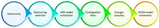
Figure 1.
The econometric framework. Source: Authors’ representation.
To prevent spurious regressions [93], it is necessary to test the stationarity of the data before estimation because non-stationary time series produce wrong results. A series stays stationary when all its properties remain constant throughout time [94]. The analysis used two tests to check stationarity namely the Augmented Dickey–Fuller (ADF) test from Dickey & Fuller [95] along with the Phillips–Perron (PP) test from Perron, Phillips & Perrson, and Leybourne & Newbold [96,97,98]. Modeling through VAR and VECM needs this property, which ensures valid inferences and stops wrong correlation identification [93,99]. This research used ADF—Fisher Chi-square and Choi Z-stat tests to determine the stationarity of E_CC_J, E_CC_J62_J63, GHG_J, and GHG_J62_J63 variables. The original data series were non-stationary based on their p-values exceeding 0.05; therefore, we created the new differenced time series of D_ECC_J, D_ECC_J62_J63, D_GHG_J, and D_GHG_J62_J63. The data passed the required tests which made it suitable for econometric modeling procedures.
Selecting optimal lag length is essential for accurate VAR or VECM estimation. Criteria used include Akaike Information Criterion (AIC) [100,101], Schwarz Bayesian Information Criterion (SBIC) [102,103], and Hannan–Quinn Criterion (HQIC) [104,105]. A VAR model was estimated using two lags to examine the dynamics among D_ECC_J, D_ECC_J62_J63, D_GHG_J, and D_GHG_J62_J63, aligning with recommendations for short time series [106]. Lag selection aimed to balance model complexity and forecasting accuracy, using standard criteria: Likelihood Ratio (LR), Final Prediction Error (FPE), Akaike / (AIC), Schwarz Criterion (SC), and Hannan–Quinn Criterion (HQ).
According to [93], the Vector Auto-Regression (VAR) model examines time series variables through models that connect variables to their own previous values and past values of other variables [93]. The model requires the conditions of both stationarity and linear relationship structure [107] together with finding the best lag structure. This study confirmed the 1-lag VAR model after running the stability check through the characteristic polynomial test [106]. The model interpretation process relied on analyzing coefficient significance, and it explained the percentage of variance through R2 while examining statistical errors through Sum sq. resid., S.E. equation. The models were validated through the assessment of Akaike Information Criterion (AIC) and Schwarz Criterion (SC).
The indication of cointegration between non-stationary variables verifies their stable long-term relationships [108]. The Johansen Test [109] detected cointegrating vectors with a lag length of two, indicating long-term connections between first-order difference variables. Analysis through the Kao Residual Test [110] proved the existence of cointegration between the variables in the balanced panel data. This evidence supported the application of a Vector Error Correction Model (VECM) for its ability to analyze short-term effects with long-term equilibrium adjustments.
The Granger causality test was applied to assess the directional relationship between cloud computing adoption and GHG emissions [111]. This method evaluates whether past values of one variable help predict another, indicating predictive causality. The test identified significant causal links and the intensity of these relationships through statistically significant coefficients. These findings provide insight into the dynamic interactions between variables and support conclusions on their short- and long-term relationships.
A presence of cointegration requires the utilization of the Vector Error Correction Model (VECM) since this model combines short-term dynamics with long-run equilibrium structures [108]. The Vector Error Correction Model contains an error correction term (ECT) that reveals how fast variables return to equilibrium status when encountering disturbances [109]. The model functions best to analyze environmentally related effects which occur gradually from technological shifts including cloud computing adoption.
The VECM estimation revealed cointegration by Johansen and Kao tests [110] while it evaluated both immediate and prolonged relationships between variables. The following two approaches made this interpretation more transparent. According to Sims [107], IRFs present the relationship of a single shock propagation throughout the system at different points in time. The sequence starts with increased GHG emissions resulting from cloud adoption energy consumption and then transitions to emission reduction through efficiency improvements and renewable resource transition.
Researchers employ variance decomposition to establish the degree to which forecast variability of individual variables results from external shock influences [106]. Research using this method enables scientists to locate the principal source between cloud computing and additional environmental factors that affect emission variations. This study used VECM to analyze the dynamic link between cloud computing and GHG emissions through IRFs and variance decomposition results which produced crucial information needed for sustainable digital policy development.
A detailed description of the econometric framework is presented in Appendix C.
4. Results
4.1. Stationarity Analysis Results
Stationarity tests applied to the four variables (E_CC_J, E_CC_J62_J63, GHG_J, GHG_J62_J63) showed that all raw series have unit roots, indicating non-stationarity (p-value > 0.05). To meet the requirements of the econometric analysis, each series was differetiated, and stationarity was confirmed after transformation (Table 3).
Table 3.
Results of ADF and Choi Z-stat tests for raw and differenced series.
To assess the stationarity of the series used in the econometric analysis, ADF (Fisher Chi-square) and Choi Z-stat stationarity tests were applied to both raw and differenced series. Appendix D provides full details of the results of the ADF and Choi Z-stat tests and includes a detailed description of each variable analyzed.
All analyzed variables became stationary after differentiation, which allows their use in Granger causality tests and VAR econometric models. The results indicate that data transformations are necessary for valid econometric analysis.
4.2. Optimal Lags Results
To identify the optimal number of lags in the VAR model, the standard econometric criteria were used: Likelihood Ratio (LR), Final Prediction Error (FPE), Akaike Information Criterion (AIC), Schwarz Criterion (SC) and Hannan–Quinn Criterion (HQ). The analysis started with a model initially configured at two lags, according to methodological recommendations for short time series [106].
The econometric criteria were applied to the first-order differentiated data. Among the five criteria, the optimal lag of three was chosen based on AIC, on the minimum recorded, which is the most appropriate to avoid overestimation of the parameters and ensure the stability of the model. However, stability tests revealed the model’s instability, with some eigenvalues exceeding the unit circle. The lag was reduced to 1 to ensure model robustness, aligning with BIC recommendations and improving stability in impulse response functions and residual diagnostics. This decision follows established econometric guidelines [86,87] and prevents overfitting, ensuring reliable inference. Appendix E presents a comparative table of the criteria values for different lags. Even so, the optimal lag of 1 was finally selected to ensure a stable model, and its results were used in the subsequent stages of the econometric analysis.
4.3. VAR Model Estimation Results
The VAR model was estimated to analyze the dynamic relationships between the included variables: D_ECC_J, D_ECC_J62_J63, D_GHG_J and D_GHG_J62_J63. The configuration of the VAR model started with a maximum of 3 lags, according to the initial selection based on econometric criteria (AIC, SC, HQ, FPE, and LR) (Appendix F, Table A2).
Although the econometric criteria indicated lag 3 as optimal, the stability analysis revealed that the model could not maintain consistency with three lags (Appendix F, Figure A2). The stability check was performed by analyzing the roots of the characteristic polynomial. Some of them had modules greater than or equal to 1, which indicates the model’s instability.
The number of lags was reduced to obtain a stable model, estimating the model for 1 and 2 lags. The econometric analysis confirms the stability of the 1-lag model (Appendix F, Table A3, Figure A3). All characteristic polynomial roots are within the unit circle, indicating that shocks dissipate over time and that the system is dynamically stable. Furthermore, the descriptive statistics reveal a high degree of variability in GHG emissions across sectors, with skewness values suggesting the presence of extreme outliers in certain regions. These disparities underline the need for targeted policies that address sectoral and regional differences in energy consumption and cloud computing adoption. This stability allows the model to be used for further analyses, such as IRF and variance decomposition, without the risk of generating uncertain results.
The estimation results highlight significant and insignificant relationships between the analyzed variables, reflecting the complexity of their dynamics. The R-squared and Adj. R-squared values suggest a moderate capacity of the model to explain the variations in the variables, being more pronounced for GHG. At the same time, the low values of the residuals and standard errors for these variables indicate a precise adjustment and good quality of the prediction.
Therefore, the choice of one-lag proved appropriate, providing a balance between the complexity of the model and the interpretability of the results. This model can be used to analyze the dynamic relationships between the variables in the short term, contributing to the understanding of the economic and ecological mechanisms studied. However, the interpretation of the results should be performed cautiously, given the methodological limitations and the complexity of the relationships between the selected variables.
4.4. Results of Cointegration Tests
The Johansen test confirms the existence of 4 long-term equilibrium relationships, indicating a significant and stable connection between the analyzed variables. These relationships clarify the long-term link between digitalization (E_CC) and sustainability (GHG).
Based on the results, a VECM is justified for analyzing short-term adjustments to the long-term equilibrium. The identified relationships support the validity of the theoretical hypotheses regarding the connection between the selected variables.
The Johansen cointegration test demonstrated the existence of strong and stable dynamic relationships between the included variables, providing a solid foundation for subsequent econometric analyses. The full table of results is included in Appendix G, Table A4 and Table A5).
To verify the existence of long-term equilibrium relationships between the variables analyzed (D_ECC_J, D_ECC_J62_J63, D_GHG_J62_J63, D_GHG_J), two Kao cointegration tests were applied using different lags (lag 2 and lag 1). These tests analyze the residuals to determine whether the variables are cointegrated, indicating a stable long-term relationship.
The results confirm the existence of a cointegration relationship between the variables, supporting the hypothesis that they are interdependent in the long run, for lag-2. On contrary, for lag-1, no cointegration relationship was identified, suggesting that long-term adjustments are insufficient at this level.
The Kao test applied with lag 2 indicates a significant cointegration relationship between the variables, confirming their long-run stability. In contrast, the lag 1 results suggest the absence of cointegration, demonstrating the importance of proper model fit. The complete results are presented in Appendix G, Table A6 and Table A7.
4.5. Results of Causality Relationship Exploration—Granger Causality
The results of the Granger Causality test suggest a significant bidirectional causal relationship between D_GHG_J and D_GHG_J62_J63 (F-statistic = 91.5921, p < 0.001; F-statistic = 60.8104, p < 0.001). These results indicate a strong interdependence between the variables measuring greenhouse gas emissions. The full table of results is presented in Appendix H.
4.6. Results of VECM Estimation
The VECM is used to analyze both the long-run equilibrium relationships and the short-run adjustments of the included variables: D_ECC_J, D_ECC_J62_J63, D_GHG_J, and D_GHG_J62_J63. The interpretation of the coefficients and their significance is based on t-statistics, according to the criterion: if the absolute value of the t-statistic exceeds 2, the coefficient is considered statistically significant at a 95% confidence level. The results for VECM are presented in Table 4 (Appendix I, Table A8).
Table 4.
VECM estimation—cointegration equation coefficients.
A cointegration equation represents a long-run equilibrium relationship between two or more time series that, although individually non-stationary (their values vary over time without having a constant mean and variance), have a stationary linear combination (has constant statistical properties over time). This indicates that although the series may deviate from each other in the short run, a stable relationship links them in the long run [108]. The concept of cointegration is essential in econometrics because it allows for the modeling and analyzing long-run relationships between economic variables, avoiding spurious regressions that can occur when working with non-stationary series. By identifying cointegration equations, economists can better understand the long-run dynamics between variables and build models that reflect their short-run and long-run behavior [108].
A classic example is the relationship between consumption and income: although both variables may be non-stationary over time, a stationary linear combination may exist, suggesting a long-run equilibrium relationship between consumption and income.
Various methods are used to test the existence of a cointegration relationship between time series, such as the Engle–Granger test or the Johansen methodology, which helps to determine the number of cointegration relationships and estimate them [109].
The values obtained for error correction for CointEq1 are as follows:
- -
- D_ECC_J: 0.338699, t-statistics = 0.40570 (|t| < 2, insignificant).
- -
- D_ECC_J62_J63: 3.315950, t-statistics = 2.79046 (|t| > 2, significant).
- -
- D_GHG_J: 0.596205, t-statistics = 1.46592 (|t| < 2, insignificant).
- -
- D_GHG_J62_J63: 0.321727, t-statistics = 1.96138 (|t| < 2, almost significant).
Short-term adjustments to the long-term equilibrium are not significant for D_ECC_J and D_GHG_J. Short-term adjustments are significant, indicating rapid convergence towards equilibrium for D_ECC_J62_J63 and they are almost significant for D_GHG_J62_J63 which may indicate a moderate effect in short-term adjustments.
Details about the VECM estimation and analysis are presented in Appendix H.
The VECM’s performance results show an R-squared of 0.982672 and an Adjusted R-squared of 0.971532 for D_GHG_J62_J63, indicating a perfect model fit. The values for the rest of the variables are lower, suggesting a moderated variation. The values of the Durbin–Watson stat reflect an adequate level of autocorrelation for the model.
For the long term, the cointegration relationships are confirmed for D_ECC_J62_J63 and D_GHG_J, indicating significant relations with D_ECC_J, while D_GHG_J62_J63 does not significantly affect long-term equilibrium.
In the short term, the adjustments are significant for D_ECC_J62_J63, suggesting rapid convergence of this variable towards equilibrium. The other variables have weaker effects in short-term adjustments.
The results justify using the VECM to analyze the dynamic relationships between the included variables. These findings are important for understanding digitalization (E_CC) and sustainability (GHG) connections. The complete results with coefficients and statistics are presented in Appendix I, Table A8.
4.7. Impulse Response Function Results
Figure 2 provides a visual representation of the responses of the variables under analysis following an exogenous shock to another variable. The impulse response functions (IRFs) derived from the VAR and VECM estimations illustrate the dynamic responses of cloud computing adoption (E_CC) and greenhouse gas emissions (GHG) in the Information and Communication (J) and IT consultancy (J62_J63) subsectors.
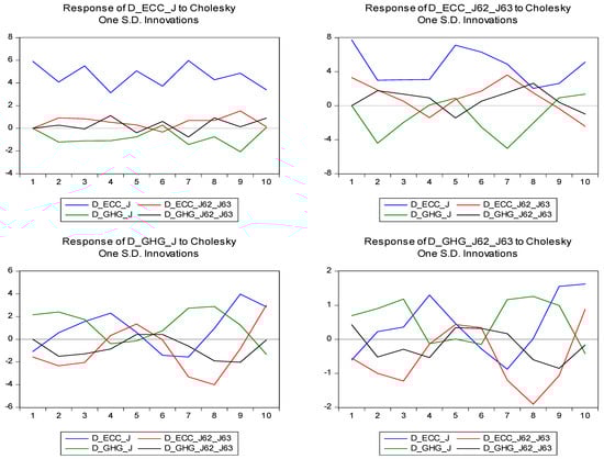
Figure 2.
Impulse response function results. Source: Research results. Detailed Legend. The slot title mentions the variable that suffers the impulse. X-axis: Represents 10 periods (years), indicating the temporal evolution of changes for the considered variables. Y-axis: Represents the change in units (percentage for cloud computing adoption and kg CO2 equivalent per capita for GHG). D_ECC_J (Blue Line)—First difference of cloud computing adoption in the entire IT and communications sector (NACE J). D_ECC_J62_J63 (Red Line)—First difference of cloud computing adoption in software development, consultancy, and information service activities (NACE J62_J63). D_GHG_J (Green Line)—First difference of GHG emissions in the entire IT and communications sector (NACE J). D_GHG_J62_J63 (Black Line)—First difference of GHG emissions in software development, consultancy, and information service activities (NACE J62_J63).
Each graph shows how the variables respond over 10 periods, where each step is equivalent to one lag. Also, the shock is applied at the initial (0 moment) in an equilibrium point of the model. Since the dataset consists of annual observations, each simulated period in the impulse response functions (IRFs) corresponds to one year. Therefore, the ten periods displayed in the IRF plots represent the system’s dynamic responses over a ten-year horizon following a one-standard-deviation shock. The IRFs illustrate the dynamic responses of all four variables to sequential one-standard-deviation shocks, applied to each variable within the model. Each graph simulates the propagation of the shock over a ten-year horizon, reflecting the interdependencies captured by the VECM framework. Each curve in the IRF plots represents the response of the change (first difference) in the respective variable to a one-standard-deviation shock. Therefore, positive or negative values indicate an increase or decrease in the rate of change, not the absolute levels of cloud adoption or emissions.
The response of the variable D_ECC_J is as follows:
- -
- D_ECC_J to its own shocks—We observe a moderate oscillation in the first 10 periods, with a tendency to return to equilibrium. This indicates that the general sector J has a strong inertia in adapting to internal shocks.
- -
- D_ECC_J62_J63 to D_ECC_J—The initial impact is positive but transitory. This suggests a complementarity relationship between the general sector and the IT subsectors.
- -
- D_GHG_J to D_ECC_J—The effects are oscillating and insignificant. This indicates that changes in the general sector’s use of cloud computing do not consistently affect overall emissions.
- -
- D_GHG_J62_J63 to D_ECC_J—The impact is weak, suggesting an indirect relationship between emissions in the IT subsectors and the general sector.
Overall, this panel indicates that accelerated digitalization drives sectoral interconnections, with positive spillovers from the general ICT sector to the IT subsectors. However, the short-term environmental impact remains modest, underscoring the potential of digital transformation to scale without immediate adverse effects on emissions. Nonetheless, sustained growth in digitalization may require careful monitoring to avoid longer-term environmental pressures [112].
The response of variable D_ECC_J62_J63 is:
- -
- D_ECC_J to D_ECC_J62_J63: Shocks in the general sector have a transitory and positive impact on IT subsectors, indicating a chain propagation effect.
- -
- D_GHG_J to D_ECC_J62_J63: The impact is initially negative but tends to become positive in the long run, suggesting a gradual adaptation of IT subsectors to shocks in general emissions.
- -
- D_GHG_J62_J63 to D_ECC_J62_J63: The positive impact confirms that IT subsectors are leaders in adapting to new technological conditions.
This dynamic highlight a potential sustainability trade-off: although digitalization can improve efficiency initially, the long-term environmental impact may be negative if not accompanied by green infrastructure investments and energy-efficiency policies. This observation is consistent with Barteková and Börkey [113], who emphasize that the environmental benefits of digital technologies depend heavily on targeted policies ensuring resource efficiency and minimizing rebound effects.
The response of variable D_GHG_J is:
- -
- D_ECC_J to D_GHG_J: The impact is marginal, suggesting that cloud computing does not significantly reduce general emissions.
- -
- D_GHG_J62_J63 to D_GHG_J: Shocks in IT subsectors moderate overall emissions, reflecting an indirect relationship between the two.
This panel reveals complex feedbacks: while general emissions growth shocks trigger immediate defensive responses in the IT sector, these adjustments fade, and both emissions and digitalization growth rates tend to stabilize. The limited long-term response of digitalization variables confirms a decoupling: rising environmental pressures do not substantially alter the digital adoption trajectory, especially without targeted policy interventions [114].
The response of variable D_GHG_J62_J63 is:
- -
- D_ECC_J62_J63 to D_GHG_J62_J63: IT subsectors show a transitory reduction in emissions, reflecting the technological efficiency of cloud computing infrastructure.
- -
- D_GHG_J to D_GHG_J62_J63: The impact is positive and consistent, indicating that overall emissions directly influence IT subsectors.
Overall, this panel confirms the asymmetric relationship between digitalization and emissions dynamics: while GHG emission shocks in the IT subsector spill over to the general sector, digitalization growth is less sensitive to environmental pressures. The results highlight the need for targeted policies to better align digital expansion with environmental objectives and prevent potential rebound effects where increased IT activity might fuel emissions growth in the absence of green infrastructure [114].
The response of each variable after a shock in other variables was estimated.
Period 1 reflects the immediate impact. In our case, general emissions (D_GHG_J) and IT subsectors (D_GHG_J62_J63) have a weak initial response to general sector shocks, indicating a slow propagation of effects. IT subsectors (D_ECC_J62_J63) show an immediate and positive response to their shocks, indicating their inertia and stability.
The persistence of effects is reflected by periods 2–10. Shocks in D_GHG_J and D_GHG_J62_J63 tend to generate oscillating responses in D_ECC_J and D_ECC_J62_J63 variables, suggesting a gradual adaptation of the IT sector to sustainability requirements. Oscillations progressively decrease, indicating that the system tends to return to equilibrium.
The sign of the answer gives information about the generated effect. A shock in D_ECC_J62_J63 causes a transient decrease in D_GHG_J62_J63, confirming a positive effect on sustainability.
Considering the responses of the variables, the economic and political implications can be formulated. Cloud computing technologies have the potential to reduce emissions in IT subsectors, but their effects on overall emissions are limited. The transitory and indirect effects between variables suggest that better coordination between sustainability and digitalization policies is needed. IT subsectors respond positively and quickly to shocks, justifying investments in green technologies and cloud infrastructures.
Appendix I, Table A9 and Figure A4 highlights the complexity of the relationships between cloud computing use (D_ECC_J, D_ECC_J62_J63) and greenhouse gas emissions (D_GHG_J, D_GHG_J62_J63). The IRF chart and table highlight both digitalization’s positive effects and limitations in the green transition, suggesting that the IT sector can catalyze sustainability. However, additional measures are needed to maximize the impact.
4.8. Results of Variance Decomposition
Variance decomposition is a fundamental econometric tool used to determine the contribution of each variable to the total variations in the system of equations. This helps us understand how much of the variation in each variable is explained by its own shocks and how much by the others in the system [106]. This method shows the relationships between cloud computing adoption and greenhouse gas (GHG) emissions in both the general ICT sector and IT-specific activities.
This analysis identifies the main sources of variation in the dynamics of the variables included in the model, highlighting the degree of influence of endogenous variables on the other components. In this case, the analysis focuses on four variables: D_ECC_J, D_ECC_J62_J63, D_GHG_J, and D_GHG_J62_J63, representing the use of cloud computing and greenhouse gas emissions in different sectors.
Like the impulse response functions, the variance decomposition analysis uses 10 simulated periods, each corresponding to one year, given the dataset’s annual frequency. In Figure 3, the x-axis represents these 10 simulation periods (years), showing how the proportion of variance explained by each variable evolves. The y-axis indicates the percentage contribution of each variable’s shocks to the forecast error variance of the target variable. Each line in the graph traces each variable growing or decreasing in influence on the system’s dynamics across the 10-year simulation horizon. This setup allows us to assess both short-term and long-term influences within the system. It reflects the interdependencies and feedback effects between cloud computing adoption and greenhouse gas emissions, consistent with the model’s annual data structure.
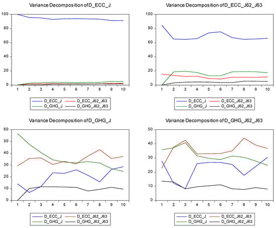
Figure 3.
Variance decomposition for the VECM variables. Source: Research results. Detailed Legend: The slot title mentions the variable considered for decomposition. X-axis: Represents 10 periods (years), indicating the temporal evolution of changes for the considered variables. Y-axis: Represents the units (percentage for cloud computing adoption and kg CO2 equivalent per capita for GHG). D_ECC_J (Blue Line)—First difference of cloud computing adoption in the entire IT and communications sector (NACE J). D_ECC_J62_J63 (Red Line)—First difference of cloud computing adoption in software development, consultancy, and information service activities (NACE J62_J63). D_GHG_J (Green Line)—First difference of GHG emissions in the entire IT and communications sector (NACE J). D_GHG_J62_J63 (Black Line)—First difference of GHG emissions in software development, consultancy, and information service activities (NACE J62_J63).
Table 5.
Variance decomposition.
Variance decomposition results emphasize the need for digitalization and targeted support policies, along with sectoral integration and strategic planning. The results show that cloud computing can influence emission reduction but with different effects across sectors [113,114]. Policies should support investments in energy-efficient IT infrastructures. The interaction between the general sector and IT subsectors is essential for implementing the green transition. Cloud expansion in IT subsectors increasingly contributes to general emission dynamics, confirming that unchecked digitalization may drive emissions growth unless supported by green infrastructure [112,114]. Better coordination could amplify the impact of digitalization on sustainability. Investments in research and development for sustainable IT infrastructures are essential [115]. The results emphasize the importance of using digital technologies to reduce emissions.
Figure 3 and Table 5 highlight the complex dynamics between cloud computing and greenhouse gas emissions. The variance decomposition highlights the dominant role of autoregressive shocks in the model but also the important, albeit gradual, influence of the other variables. The results support the idea that digital technologies can contribute to reducing emissions, but implementing these solutions requires integrated policies and consistent investments in sustainable infrastructure.
These results confirm that while self-dependence dominates, cross-sector effects grow over time. The findings highlight the need for policies that integrate digitalization and sustainability goals [114,116]. Investments in energy-efficient cloud infrastructure and support for the IT sector’s green transition are essential to maximize digitalization’s contribution to emission reduction.
5. Discussion
This study demonstrates how digitalization contributes to carbon footprint reduction, offering empirical support for sustainable digital policies. Adopting cloud computing services in IT subsectors provides an example of good practice, suggesting opportunities for replication in other economic sectors.
The study hypotheses were validated, as presented in Table 6, based on the results of the VAR and VECMs.
Table 6.
Hypotheses validation.
The VAR and VECMs proposed for analyzing the correlation between cloud computing use and GHG emissions reflect a potential methodologic framework to evaluate the impact of digitalization on energy and mass transfer.
A synthesis of the original contributions of our study are listed below:
- (a)
- This study combines econometric analysis (cointegration, Granger tests) with mass and energy flow theory to understand the relationship between digitalization and sustainability, representing an innovative interdisciplinary approach.
- (b)
- This research provides a detailed analysis of sectoral differences in the use of cloud computing services and the impact on GHG emissions, with a focus on the IT subsectors (J62_J63). This level of detail is rarely found in the literature.
- (c)
- We used advanced VECM and impulse-response functions to explore short-term adjustments towards long-term equilibrium, complemented by impulse-response functions and variance decomposition to understand the dynamics and interdependencies between variables.
- (d)
- This study provides empirical evidence that cloud computing services can reduce GHG emissions in the IT sectors, underscoring the critical role of digitalization in the green transition. Similar studies for various variables can support policy relevance for the twin transition (green and digital).
- (e)
- This research uses recent data (2014–2021) and relevant economic variables, such as GHG emissions and the use of cloud computing services, to provide an up-to-date picture of the impact of digital technologies.
- (f)
- We have shown that IT subsectors (J62_J63) are more efficient in using digital technologies to optimize mass and energy flows compared to the overall communications sector (J), making a key contribution to understanding structural differences between sectors.
- (g)
- This study extends the use of econometric models to include a physical perspective on mass and energy flows, laying the foundation for further interdisciplinary research.
These contributions add value to the existing literature and provide a solid empirical and theoretical framework for sustainability-oriented public policies.
6. Conclusions
6.1. Impact of Cloud Computing on GHG Emissions
The use of cloud computing significantly contributes to the optimization of mass and energy flows, reducing greenhouse gas (GHG) emissions in the IT subsectors (J62_J63). This highlights the superior energy efficiency of these subsectors, due to advanced digitalization and modern infrastructures. In the general communications sector (J), the impact is lower, suggesting a slower and less efficient adoption of digital technologies.
Granger causality tests reveal no direct causal link between cloud computing adoption (E_CC) and GHG emissions. However, a strong bidirectional causality exists between GHG emissions in the general communications sector (D_GHG_J) and IT subsectors (D_GHG_J62_J63), highlighting interdependencies between these emission sources.
Cointegration tests and the VECM showed a stable long-run relationship between cloud computing and GHG emissions, highlighting the digital transition’s potential to support sustainability.
IT subsectors (J62_J63) demonstrated a higher adjustment capacity to shocks in cloud computing use. At the same time, the general sector (J) had a more extended adjustment period and a reduced impact on emissions. ITFs suggest that shocks in cloud computing adoption can influence GHG emissions in IT subsectors (J62_J63), but the effect varies over time and is contingent upon sectoral energy efficiency and infrastructure optimization. However, the effects are delayed and less pronounced in the broader communications sector, indicating the need for tailored policies that address sector-specific dynamics and barriers to technology adoption.
Variance decomposition shows that digitalization-related variables (D_ECC_J and D_ECC_J62_J63) contribute significantly to long-term emission variations, highlighting the role of cloud technologies in optimizing resource flows.
Digitalization plays a crucial role in supporting the green transition, but its impact depends on the energy sources used and the level of adoption of green technologies in each sector. IT subsectors can serve as a model for the rapid and efficient adoption of digital technologies in other sectors. The transition to centralized infrastructures, such as data centers, optimizes mass and energy flows, reducing the environmental impact of local IT solutions. However, these advantages can be mitigated by negative externalities, such as the increased overall energy consumption of data centers.
6.2. Research Question Answer
Based on the results from Granger causality tests, VAR, VECM, variance decomposition, and impulse response functions, this study provides answer for the research question of this study.
Cloud computing adoption (E_CC) does not directly and immediately impact GHG emissions. Granger causality tests show no statistically significant short-term relationship between cloud computing adoption and emissions across IT and communications sectors (H1 partially validated). This suggests that increased cloud computing usage alone does not lead to an automatic reduction or increase in GHG emissions.
However, strong interdependencies exist between greenhouse gas emissions in the general communications sector (J) and IT subsectors (J62_J63). A strong bidirectional Granger causality (p < 0.001) was found between D_GHG_J and D_GHG_J62_J63, meaning emissions in these sectors influence each other dynamically. This interconnection suggests that emission trends in IT subsectors are partially driven by broader industry-wide factors, such as energy demand, infrastructure efficiency, and digitalization policies.
Sectoral differences in cloud computing’s impact on emissions are significant. IT subsectors (J62_J63) demonstrate more efficient use of digital infrastructure, leading to potential energy optimizations over time, whereas the general communications sector (J) has a slower adaptation process (H3, H4 validated). The variance decomposition analysis confirms that cloud computing plays a role in shaping long-term energy use patterns, particularly in IT-intensive industries.
Cloud computing contributes to changes in mass and energy flows, but its direct impact on GHG reductions remains inconclusive. Cloud computing adoption influences energy and mass flows across the sector, but its role in emissions reduction is dependent on sectoral efficiency, renewable energy integration, and data center optimization (H2 validated).
The optimal lag for assessing cloud computing’s effect on emissions varies. While lag 3 is best suited for long-term equilibrium adjustments, shorter lags (1–2) explain short-term fluctuations better (H5 partially validated). These findings suggest that cloud computing’s environmental impact unfolds gradually over time, rather than producing immediate changes.
Thus, this study concludes that cloud computing adoption does not have an immediate causal effect on GHG emissions but influences long-term energy optimization, particularly in IT-intensive sectors. These insights highlight the need for tailored digitalization and sustainability policies to maximize environmental benefits.
This research answers the question of how cloud computing affects mass and energy flows, measured by GHG emissions, in the IT and communications sectors in Europe (2014–2021). The findings confirm that cloud adoption does not directly cause emissions reductions in the short term but plays a key role in shaping long-term energy efficiency patterns, particularly in IT-intensive industries.
The strong sectoral interdependence of emissions highlights the need for targeted sustainability strategies, while optimal lag structure analysis suggests that cloud computing’s full impact on emissions emerges over extended timeframes.
6.3. Study Limits
This study uses data from 2014 to 2021, excluding 2019, which limits the analysis of long-term trends and the full impact of cloud adoption on emissions. Some countries or sectors may have incomplete data, affecting the generalizability of the results. Econometric models, such as VECM, assume stationarity and cointegration of variables. Results may be influenced by the selection of lags and the order of variables in the Cholesky analysis. This study does not include external variables, such as emissions regulations or direct investments in green infrastructure, that could influence the results.
6.4. Further Developments
Integrating data over a longer period of time and updating datasets will allow for a deeper understanding of the impact of cloud adoption on emissions and the economy. Extending the analysis to other economic sectors, such as transport or energy, would provide a more complete perspective on the interdependence between digitalization and sustainability. Adding variables such as environmental regulations, R&D investments and energy policies could better explain the dynamics between digitalization and GHG emissions. Investigating regional or national variations to identify specificities of cloud adoption and the impact on emissions. Integrating perspectives from physics, social sciences, and technological studies for a deeper understanding of mass and energy flows and the implications for sustainability.
Moreover, COVID-19 acted as a booster for the digital transformation and adoption of cloud computing services. Sensitivity analysis and structural break tests about digital transformation, cloud computing services, AI adoption, etc., are topics of interest.
Author Contributions
Conceptualization, A.G., C.L. and C.S.P.; methodology, A.G., C.L. and C.S.P.; software, C.L.; validation, A.G. and C.S.P.; formal analysis, C.L. and C.S.P.; investigation, C.L.; resources, C.S.P.; data curation, C.L.; writing—original draft preparation, A.G., and C.L.; writing—review and editing, A.G. and C.S.P.; visualization, C.L. and A.G.; supervision, A.G. and C.S.P.; project administration, A.G.; funding acquisition, C.S.P. All authors have read and agreed to the published version of the manuscript.
Funding
This research was funded by the Romanian Ministry of Research, Innovation, and Digitalization, Program NUCLEU, 2022–2026, PN 22_10_0105.
Data Availability Statement
Data used are from public sources mentioned in the main text.
Acknowledgments
This work was supported by a grant from the Romanian Ministry of Research, Innovation, and Digitalization, Program NUCLEU, 2022–2026, Spatio-temporal forecasting of local labour markets through GIS modelling [P5] PN 22_10_0105.
Conflicts of Interest
The authors declare no conflicts of interest.
Abbreviations
The following abbreviations are used in this manuscript:
| IT | Information technology |
| GHG | Greenhouse gas |
| VAR | Vector Auto-Regression |
| VECM | Vector Error Correction Models |
| IRF | Impulse response functions |
Appendix A. Building and Structuring the Balanced Data Panel
Table A1.
Common descriptive statistics for variables E_CC_J, E_CC_J62_J63, GHG_J and GHG_J62_J63.
Table A1.
Common descriptive statistics for variables E_CC_J, E_CC_J62_J63, GHG_J and GHG_J62_J63.
| ECC_J | ECC_J62_J63 | GHG_J | GHG_J62_J63 | |
|---|---|---|---|---|
| Mean | 51.07375 | 56.58125 | 18.11201 | 7.085123 |
| Median | 48.00000 | 54.90000 | 13.18978 | 4.140560 |
| Maximum | 93.10000 | 97.40000 | 85.58348 | 41.07625 |
| Minimum | 15.60000 | 21.80000 | 2.972950 | 1.012820 |
| Std. Dev. | 18.97992 | 18.75741 | 17.42633 | 7.916313 |
| Skewness | 0.371863 | 0.113451 | 2.222058 | 2.276262 |
| Kurtosis | 2.250468 | 2.106907 | 8.178066 | 8.290706 |
| Jarque–Bera | 3.716421 | 2.830331 | 155.2085 | 162.3901 |
| Probability | 0.155951 | 0.242885 | 0.000000 | 0.000000 |
| Sum | 4085.900 | 4526.500 | 1448.961 | 566.8098 |
| Sum Sq. Dev. | 28,458.75 | 27,795.38 | 23,990.47 | 4950.773 |
| Observations | 80 | 80 | 80 | 80 |
Note: The variables analyzed are the same as in Table 1 but calculated for a common sample of 80 observations. Source: Research results.
Appendix B. Figure A1 Detailed Explanation
The figure in the first two quadrants presents the evolution of the percentage of enterprises in the Information and Communication sector, respectively, subsectors J62 and J63 (IT programming, consulting, and other information services) that use cloud computing services and in the last two, the greenhouse gas emissions expressed in kilograms of CO2 equivalent per capita, for the same sector and subsectors (axis y—graph ordinates). The chart presents data at the NUTS 0 level, covering 14 European countries, including 12 EU member states: Bulgaria (BG), Croatia (HR), Cyprus (CY), Denmark (DK), Spain (ES), Finland (FI), Hungary (HU), Lithuania (LT), Latvia (LV), Poland (PL), Romania (RO), and Slovakia (SK), as well as two non-EU countries, and Norway (NO), including via the European Economic Area (EEA).

Figure A1.
Evolution of cloud computing use and GHG emissions in the IT and communications sectors (2014–2021). Source: Research results.
- E_CC_J graph
Variable analyzed: Percentage of enterprises in the Information and Communication sector that use cloud computing services.
- Trend: A progressive increase in the use of cloud computing services is observed in the Information and Communication sector, highlighting a constant digital transition.
- Fluctuations: Although there are periods with slight oscillations, the general trend is upward, suggesting a growing adoption of digital technologies.
- Relevance: The increase reflects the acceleration of digitalization processes in this sector, possibly correlated with public policies favorable to digitalization and improved IT infrastructures.
- E_CC_J62_J63 graph
Variable analyzed: Percentage of enterprises in subsectors J62 and J63 (IT programming, consulting and other information services) that use cloud computing services.
- Trend: The growth is similar to that of E_CC_J, but more stable, suggesting a uniform adoption of cloud services in these subsectors.
- Fluctuations: Variability is lower, which may indicate a more homogeneous behavior among enterprises in these subsectors.
- Relevance: The IT and communications subsectors are natural leaders in the adoption of cloud technologies, due to the specificity of their digital activities.
- GHG_J graph
Variable analyzed: Per capita greenhouse gas emissions for the Information and Communication sector.
- Trend: The series shows significant fluctuations, with pronounced peaks in certain periods.
- Observations:
- ○
- The peaks could reflect periods of intense growth of economic activities or inefficient use of energy resources.
- ○
- In certain periods, there is a slight downward trend, possibly due to the adoption of more energy-efficient technologies.
- Relevance: The fluctuations indicate the dependence of emissions on the energy structure and the implementation of sustainable technologies in this sector.
- GHG_J62_J63
Variable analyzed: Greenhouse gas emissions per capita for subsectors J62 and J63.
- Trend: Similar to GHG_J, but with smaller fluctuations.
- Observations:
- ○
- IT subsectors show lower emission values, suggesting a more energy-efficient infrastructure.
- ○
- Peaks are likely associated with increased economic activity or periods of high energy consumption.
- Relevance: Lower emission values indicate that digitalization can contribute to reducing environmental impacts, especially through the use of centralized cloud technologies.
- Possible correlations between the graphs:
- E_CC_J and GHG_J: The increase in the use of cloud services coincides with the reduction in fluctuations in greenhouse gas emissions, which may suggest that digitalization and the transition to more efficient IT infrastructures contribute to the decrease in emissions.
- E_CC_J62_J63 and GHG_J62_J63: The adoption of cloud technologies is more pronounced in the IT subsectors, which may explain the lower and more stable emission values in these sectors compared to the overall level of emissions in the communications sector.
- Conclusions:
- The graphs highlight an accelerated digital transition through the adoption of cloud computing services, which indirectly contributes to the reduction in greenhouse gas emissions.
- The IT and communications sector shows a positive evolution, but the fluctuations in emissions in the general sector suggest that there is still room for improvement, especially by implementing sustainable solutions.
- Relevance for research: Correlations between the use of digital technologies and greenhouse gas emissions can guide future policies for a sustainable digital economy.
Appendix C. Detailed Description of Methodology
Appendix C.1. Stationarity
Before proceeding with the estimation, it is essential to determine whether the time series variables exhibit stationarity, as non-stationary data can lead to spurious regressions [93]. A stationary time series has statistical properties—mean, variance, and autocovariance—that remain constant over time [94]. Stationarity is tested using the Augmented Dickey–Fuller (ADF) test [95] and the Phillips–Perron (PP) test [96,97,98]. Stationarity refers to a time series maintaining constant statistical properties over time, ensuring consistency in analysis. This property ensures that the behavior of the series does not change unpredictably, allowing for consistent modeling and forecasting. Stationarity is crucial for econometric models like Vector Auto-Regression (VAR) and Vector Error Correction Models (VECM) to prevent spurious correlations and ensure reliable results [93,99].
Stationarity is crucial for time series and panel data analysis. It prevents spurious correlations and ensures the validity of the econometric models used, such as the Granger causality test and the Vector Auto Regression (VAR)/Vector Error Correction Models (VECMs) [93,94]. In this study, we verified the stationarity of the four variables analyzed (E_CC_J, E_CC_J62_J63, GHG_J, GHG_J62_J63) using the ADF—Fisher Chi-square and Choi Z-stat tests, following the standard methodology [99].
The tests were applied to the raw series to assess the presence of unit roots (null hypothesis). If the series was not stationary (p-value > 0.05), first-order differentiation was applied to obtain stationarity. The same tests were applied to D_ECC_J, D_ECC_J62_J63, D_GHG_J and D_GHG_J62_J63. The results of these analyses were used to ensure the validity of subsequent econometric applications.
Appendix C.2. Selection of the Optimal Lags
Selecting the correct number of lags is crucial for ensuring the accuracy of Vector Auto-Regression (VAR) or Vector Error Correction Model (VECM) estimations. The appropriate lag length is determined using:
- -
- Akaike Information Criterion (AIC) [100,101]
- -
- Schwarz Bayesian Information Criterion (SBIC) [102,103].
- -
- Hannan–Quinn Criterion (HQIC) [104,105]
The selected lag structure balances model complexity and predictive accuracy.
The estimation of a VAR model was used to analyze the dynamic relationships between the analyzed variables: D_ECC_J, D_ECC_J62_J63, D_GHG_J, and D_GHG_J62_J63. This method allows modeling the interdependent relationships between variables, considering their lagged effects.
The analysis began with a VAR model configured at two lags, according to methodological recommendations for short data series. According to the specialized literature, choosing a small number of lags (1–2) is indicated for datasets with small temporal dimensions to avoid overestimating parameters and problems associated with model overloading [106]. To identify the optimal lag, the standard econometric criteria were applied: Likelihood Ratio (LR), Final Prediction Error (FPE), Akaike Information Criterion (AIC), Schwarz Criterion (SC), and Hannan–Quinn Criterion (HQ).
Appendix C.3. The VAR Model
The VAR model captures interdependencies among multiple time series variables, allowing for dynamic analysis [93]. Each variable is expressed as a function of its own lagged values and the lagged values of other variables in the system.
Key Assumptions of VAR:
- -
- The time series must be stationary to avoid misleading results.
- -
- The model assumes a linear interdependency between variables [107].
- -
- The lag structure must be optimized to prevent overfitting.
If variables are found to be non-stationary, the next step involves cointegration testing to determine whether a long-run equilibrium relationship exists.
Based on the previously identified optimal lag, a 3-lag VAR model was configured, and its stability was verified. In the lag structure analysis, all roots of the characteristic polynomial were evaluated to determine if their modulus was less than 1, which would confirm the model’s stability [106]. After successive checks and trials, the VAR model was observed to be stable at a lag of 1.
The stable model was interpreted by analyzing the coefficients and their statistical significance, prediction quality, and model stability. R-square was used to evaluate the model’s explanatory power. The indicators Sum sq. resides and S.E. equation were taken into account to analyze errors and variations. Additional stability was confirmed through econometric criteria such as the Akaike Information Criterion (AIC) and Schwarz Criterion (SC), which evaluate the performance of the model in relation to its complexity.
Appendix C.4. Cointegration Tests
Cointegration refers to a long-term equilibrium relationship between non-stationary variables, despite short-term fluctuations [108]. The Johansen cointegration test [109] is applied to assess:
- -
- The presence of cointegrating vectors, indicating a stable long-run relationship.
- -
- The number of cointegration equations in the system
If cointegration is detected, the VAR model is transformed into a Vector Error Correction Model (VECM) to incorporate both short-term adjustments and long-term equilibrium relationships.
A balanced panel of the first derivative of the variables was used for the cointegration analysis. For this purpose, two main tests were applied:
- (a)
- Johansen Cointegration Test: This test was applied in the first stage to evaluate long-term cointegration relationships between the 1st-order derived variables [109]. Its results confirmed the long-term dynamic relationships for lag 2, indicating that the analyzed variables are cointegrated.
- (b)
- Kao Residual Cointegration Test: This was used to validate the cointegration on the balanced panel of the first derivative. Based on the analysis of the residuals, the Kao test further confirmed the long-term relationships between the analyzed variables [110].
The presence of cointegration allowed the identification of long-term dynamic relationships, supporting the application of an appropriate econometric model for the analysis of the behavior of the variables.
Appendix C.5. Exploring the Causality—Granger Causality
To further investigate the direction of causality between cloud computing adoption and GHG emissions, the Granger causality test [111] is conducted. This test assesses whether past values of one variable significantly improve the prediction of another variable. A significant result suggests predictive causality, although it does not necessarily imply a direct causal relationship.
The causal relationships between the variables included in the model were investigated using the Granger Causality test, which assesses whether the past values of one variable can be used to predict the current values of another variable. This test determined the directions and intensity of the causal relationships between the selected variables, providing a clear perspective on their dynamic interactions [111].
The Granger test results highlighted significant causal directions between certain variables and the intensity of the causal relationships, represented by the statistical significance of the coefficients. These results contribute to understanding the causal mechanisms and support the formulation of conclusions regarding the dynamic relationships in the short and long term.
Appendix C.6. Estimation and Analysis of the VECM
When variables are cointegrated, the VECM is preferred over VAR because it integrates both short-term fluctuations and long-term equilibrium adjustments [108] and better respond to this study objectives.
Key components of VECM:
- -
- Short-Term Dynamics—Captures short-run deviations from equilibrium.
- -
- Error Correction Term (ECT)—Represents the speed at which variables revert to their long-run equilibrium [109].
The VECM is particularly useful in cases where technological advancements, such as cloud computing adoption, lead to gradual environmental impacts over time.
The VECM analyzed both short-run adjustments and long-run relationships between variables. The estimation of the VECM was based on the confirmation of cointegration relationships. Cointegration tests (Johansen and Kao Residual Cointegration) demonstrated the existence of a significant long-run relationship between the derived variables. Also, the VECM allows the evaluation of the process by which variables adjust and converge towards long-run equilibrium after being subjected to shocks or deviations. To enhance the interpretability of the VECM, two key subroutines are used: impulse response functions (IRF) and variance decomposition.
(A) Impulse response functions (IRFs) analyze how a shock to one variable propagates throughout the system and influences other variables over time [107]. In this study, IRFs are used to examine the dynamic effects of a sudden increase in cloud computing adoption on GHG emissions:
- -
- A positive shock in cloud computing adoption may initially lead to higher GHG emissions due to increased energy demand.
- -
- Over time, efficiency gains and the transition to renewable energy sources could lead to a reduction in emissions.
IRFs provide temporal insights, illustrating how different variables adjust over time following an external shock. IRF analysis was applied to assess the impact of a shock on a variable in the system and how it propagates to the other variables in the model. This analysis provides essential information about the direction, magnitude, and duration of dynamic influences in the studied system.
(B) Variance decomposition quantifies the proportion of a variable’s forecast error variance that can be attributed to shocks in other variables in the system [106]. In the context of this study, variance decomposition helps identify:
- -
- The primary drivers of GHG emissions variations (e.g., cloud adoption, economic activity, and energy mix).
- -
- The extent to which cloud computing adoption explains fluctuations in emissions compared to other external shocks.
This method provides valuable insights into policy implications, helping stakeholders prioritize interventions that could reduce emissions while fostering digital transformation. Variance decomposition was used to measure each variable’s contribution to the overall system variations. This method allows the identification of variables that have the greatest impact on explaining the system’s fluctuations over different time horizons.
The VECM provided a robust framework for analyzing the relationships between variables, allowing not only the identification of short-term adjustments and long-term relationships but also the assessment of dynamic shocks and the contribution of variables to the system’s variations.
VAR and VECM Frameworks were the proper approach for this study because VAR Models are effective for short-term forecasting and dynamic analysis and VECMs provide additional depth by integrating both short-term deviations and long-term equilibrium adjustments. Moreover, IRFs and variance decomposition offer a more detailed view of how cloud computing adoption influences environmental sustainability.
By employing VAR, VECM, and subroutines like IRFs and variance decomposition, this study delivers a comprehensive econometric analysis of cloud computing’s impact on GHG emissions, offering valuable insights for policy development and sustainable technology adoption.
Appendix D. Results of the Stationary Tests (ADF and Choi Z-Stat) for Raw and Differenced Series
- Stationarity test for ECC_J
| Null Hypothesis: Unit root (individual unit root process) | ||||
| Series: ECC_J | ||||
| Date: 01/07/25 Time: 22:03 | ||||
| Sample: 2014 2021 | ||||
| Exogenous variables: Individual effects | ||||
| Automatic selection of maximum lags | ||||
| Automatic lag length selection based on SIC: 0 | ||||
| Total (balanced) observations: 84 | ||||
| Cross-sections included: 14 | ||||
| Method | Statistic | Prob.** | ||
| ADF—Fisher Chi-square | 8.51050 | 0.9999 | ||
| ADF—Choi Z-stat | 3.31014 | 0.9995 | ||
| ** Probabilities for Fisher tests are computed using an asymptotic Chi-square distribution. All other tests assume asymptotic normality. | ||||
| Intermediate ADF test results ECC_J | ||||
| Cross | ||||
| section | Prob. | Lag | Max Lag | Obs |
| BG | 0.8627 | 0 | 0 | 6 |
| CY | 0.9493 | 0 | 0 | 6 |
| DK | 0.7826 | 0 | 0 | 6 |
| ES | 0.2283 | 0 | 0 | 6 |
| FI | 0.5227 | 0 | 0 | 6 |
| HR | 0.9323 | 0 | 0 | 6 |
| HU | 0.6444 | 0 | 0 | 6 |
| LT | 0.7521 | 0 | 0 | 6 |
| LV | 0.9169 | 0 | 0 | 6 |
| NO | 0.7556 | 0 | 0 | 6 |
| PL | 0.9648 | 0 | 0 | 6 |
| RO | 0.8464 | 0 | 0 | 6 |
| SI | 0.8808 | 0 | 0 | 6 |
| SK | 0.8239 | 0 | 0 | 6 |
| Source: Extract from EViews application. | ||||
- 2.
- Stationarity test for D_ECC_J
| Null Hypothesis: Unit root (individual unit root process) | ||||
| Series: D_ECC_J | ||||
| Date: 01/07/25 Time: 22:05 | ||||
| Sample: 2014 2021 | ||||
| Exogenous variables: Individual effects | ||||
| Automatic selection of maximum lags | ||||
| Automatic lag length selection based on SIC: 0 | ||||
| Total (balanced) observations: 70 | ||||
| Cross-sections included: 14 | ||||
| Method | Statistic | Prob.** | ||
| ADF—Fisher Chi-square | 59.9117 | 0.0004 | ||
| ADF—Choi Z-stat | −4.05170 | 0.0000 | ||
| ** Probabilities for Fisher tests are computed using an asymptotic Chi-square distribution. All other tests assume asymptotic normality. | ||||
| Intermediate ADF test results D_ECC_J | ||||
| Cross | ||||
| section | Prob. | Lag | Max Lag | Obs |
| BG | 0.0785 | 0 | 0 | 5 |
| CY | 0.2463 | 0 | 0 | 5 |
| DK | 0.2854 | 0 | 0 | 5 |
| ES | 0.1393 | 0 | 0 | 5 |
| FI | 0.1216 | 0 | 0 | 5 |
| HR | 0.1930 | 0 | 0 | 5 |
| HU | 0.1982 | 0 | 0 | 5 |
| LT | 0.1869 | 0 | 0 | 5 |
| LV | 0.0065 | 0 | 0 | 5 |
| NO | 0.0133 | 0 | 0 | 5 |
| PL | 0.3077 | 0 | 0 | 5 |
| RO | 0.5130 | 0 | 0 | 5 |
| SI | 0.0574 | 0 | 0 | 5 |
| SK | 0.1870 | 0 | 0 | 5 |
| Source: Extract from EViews application. | ||||
- 3.
- Stationarity test for ECC_J62_J63
| Null Hypothesis: Unit root (individual unit root process) | ||||
| Series: ECC_J62_J63 | ||||
| Date: 01/07/25 Time: 22:09 | ||||
| Sample: 2014 2021 | ||||
| Exogenous variables: Individual effects | ||||
| Automatic selection of maximum lags | ||||
| Automatic lag length selection based on SIC: 0 | ||||
| Total number of observations: 67 | ||||
| Cross-sections included: 12 (2 dropped) | ||||
| Method | Statistic | Prob.** | ||
| ADF—Fisher Chi-square | 21.7307 | 0.5953 | ||
| ADF—Choi Z-stat | 1.73179 | 0.9583 | ||
| ** Probabilities for Fisher tests are computed using an asymptotic Chi-square distribution. All other tests assume asymptotic normality. | ||||
| Intermediate ADF test results ECC_J62_J63 | ||||
| Cross | ||||
| section | Prob. | Lag | Max Lag | Obs |
| BG | 0.8398 | 0 | 0 | 6 |
| CY | 0.8040 | 0 | 0 | 6 |
| DK | 0.7067 | 0 | 0 | 6 |
| ES | Dropped from Test | |||
| FI | Dropped from Test | |||
| HR | 0.0003 | 0 | 0 | 3 |
| HU | 0.6916 | 0 | 0 | 6 |
| LT | 0.7753 | 0 | 0 | 4 |
| LV | 0.6493 | 0 | 0 | 6 |
| NO | 0.7960 | 0 | 0 | 6 |
| PL | 0.9367 | 0 | 0 | 6 |
| RO | 0.7717 | 0 | 0 | 6 |
| SI | 0.9532 | 0 | 0 | 6 |
| SK | 0.7371 | 0 | 0 | 6 |
| Source: Extract from EViews application. | ||||
- 4.
- Stationarity test for D_ECC_J62_J63
| Null Hypothesis: Unit root (individual unit root process) | ||||
| Series: D_ECC_J62_J63 | ||||
| Date: 01/07/25 Time: 22:15 | ||||
| Sample: 2014 2021 | ||||
| Exogenous variables: Individual effects | ||||
| Automatic selection of maximum lags | ||||
| Automatic lag length selection based on SIC: 0 | ||||
| Total number of observations: 53 | ||||
| Cross-sections included: 11 (3 dropped) | ||||
| Method | Statistic | Prob.** | ||
| ADF—Fisher Chi-square | 48.8843 | 0.0008 | ||
| ADF—Choi Z-stat | −3.71463 | 0.0001 | ||
| ** Probabilities for Fisher tests are computed using an asymptotic Chi-square distribution. All other tests assume asymptotic normality. | ||||
| Intermediate ADF test results D_ECC_J62_J63 | ||||
| Cross | ||||
| section | Prob. | Lag | Max Lag | Obs |
| BG | 0.1404 | 0 | 0 | 5 |
| CY | 0.5053 | 0 | 0 | 5 |
| DK | 0.2390 | 0 | 0 | 5 |
| ES | Dropped from Test | |||
| FI | Dropped from Test | |||
| HR | Dropped from Test | |||
| HU | 0.1730 | 0 | 0 | 5 |
| LT | 0.3000 | 0 | 0 | 3 |
| LV | 0.0043 | 0 | 0 | 5 |
| NO | 0.0348 | 0 | 0 | 5 |
| PL | 0.2454 | 0 | 0 | 5 |
| RO | 0.1383 | 0 | 0 | 5 |
| SI | 0.0418 | 0 | 0 | 5 |
| SK | 0.1287 | 0 | 0 | 5 |
| Source: Extract from EViews application. | ||||
- 5.
- Stationarity tests for GHG_J
| Null Hypothesis: Unit root (individual unit root process) | ||||
| Series: GHG_J | ||||
| Date: 01/07/25 Time: 22:29 | ||||
| Sample: 2014 2021 | ||||
| Exogenous variables: Individual effects | ||||
| Automatic selection of maximum lags | ||||
| Automatic lag length selection based on SIC: 0 | ||||
| Total (balanced) observations: 84 | ||||
| Cross-sections included: 14 | ||||
| Method | Statistic | Prob.** | ||
| ADF—Fisher Chi-square | 33.1635 | 0.2298 | ||
| ADF—Choi Z-stat | −0.50726 | 0.3060 | ||
| ** Probabilities for Fisher tests are computed using an asymptotic Chi-square distribution. All other tests assume asymptotic normality. | ||||
| Intermediate ADF test results GHG_J | ||||
| Cross | ||||
| section | Prob. | Lag | Max Lag | Obs |
| BG | 0.4643 | 0 | 0 | 6 |
| CY | 0.2820 | 0 | 0 | 6 |
| DK | 0.2421 | 0 | 0 | 6 |
| ES | 0.5681 | 0 | 0 | 6 |
| FI | 0.0026 | 0 | 0 | 6 |
| HR | 0.7608 | 0 | 0 | 6 |
| HU | 0.7270 | 0 | 0 | 6 |
| LT | 0.4752 | 0 | 0 | 6 |
| LV | 0.1072 | 0 | 0 | 6 |
| NO | 0.6663 | 0 | 0 | 6 |
| PL | 0.3726 | 0 | 0 | 6 |
| RO | 0.8272 | 0 | 0 | 6 |
| SI | 0.2432 | 0 | 0 | 6 |
| SK | 0.9583 | 0 | 0 | 6 |
| Source: Extract from EViews application. | ||||
- 6.
- Stationarity test for D_GHG_J
| Null Hypothesis: Unit root (individual unit root process) | ||||
| Series: D_GHG_J | ||||
| Date: 01/07/25 Time: 22:31 | ||||
| Sample: 2014 2021 | ||||
| Exogenous variables: Individual effects | ||||
| Automatic selection of maximum lags | ||||
| Automatic lag length selection based on SIC: 0 | ||||
| Total (balanced) observations: 70 | ||||
| Cross-sections included: 14 | ||||
| Method | Statistic | Prob.** | ||
| ADF—Fisher Chi-square | 59.5594 | 0.0005 | ||
| ADF—Choi Z-stat | −3.97682 | 0.0000 | ||
| ** Probabilities for Fisher tests are computed using an asymptotic Chi-square distribution. All other tests assume asymptotic normality. | ||||
| Intermediate ADF test results D_GHG_J | ||||
| Cross | ||||
| section | Prob. | Lag | Max Lag | Obs |
| BG | 0.2346 | 0 | 0 | 5 |
| CY | 0.0895 | 0 | 0 | 5 |
| DK | 0.4002 | 0 | 0 | 5 |
| ES | 0.0615 | 0 | 0 | 5 |
| FI | 0.0138 | 0 | 0 | 5 |
| HR | 0.2023 | 0 | 0 | 5 |
| HU | 0.1199 | 0 | 0 | 5 |
| LT | 0.6240 | 0 | 0 | 5 |
| LV | 0.1013 | 0 | 0 | 5 |
| NO | 0.0441 | 0 | 0 | 5 |
| PL | 0.3938 | 0 | 0 | 5 |
| RO | 0.1975 | 0 | 0 | 5 |
| SI | 0.1843 | 0 | 0 | 5 |
| SK | 0.0169 | 0 | 0 | 5 |
| Source: Extract from EViews application. | ||||
- 7.
- Stationarity test for GHG_J62_J63
| Null Hypothesis: Unit root (individual unit root process) | ||||
| Series: GHG_J62_J63 | ||||
| Date: 01/07/25 Time: 22:33 | ||||
| Sample: 2014 2021 | ||||
| Exogenous variables: Individual effects | ||||
| Automatic selection of maximum lags | ||||
| Automatic lag length selection based on SIC: 0 | ||||
| Total (balanced) observations: 84 | ||||
| Cross-sections included: 14 | ||||
| Method | Statistic | Prob.** | ||
| ADF—Fisher Chi-square | 31.2682 | 0.3053 | ||
| ADF—Choi Z-stat | −0.34295 | 0.3658 | ||
| ** Probabilities for Fisher tests are computed using an asymptotic Chi-square distribution. All other tests assume asymptotic normality. | ||||
| Intermediate ADF test results GHG_J62_J63 | ||||
| Cross | ||||
| section | Prob. | Lag | Max Lag | Obs |
| BG | 0.0232 | 0 | 0 | 6 |
| CY | 0.9782 | 0 | 0 | 6 |
| DK | 0.1046 | 0 | 0 | 6 |
| ES | 0.7682 | 0 | 0 | 6 |
| FI | 0.2865 | 0 | 0 | 6 |
| HR | 0.5767 | 0 | 0 | 6 |
| HU | 0.3843 | 0 | 0 | 6 |
| LT | 0.4147 | 0 | 0 | 6 |
| LV | 0.0987 | 0 | 0 | 6 |
| NO | 0.6489 | 0 | 0 | 6 |
| PL | 0.3972 | 0 | 0 | 6 |
| RO | 0.8431 | 0 | 0 | 6 |
| SI | 0.1790 | 0 | 0 | 6 |
| SK | 0.8794 | 0 | 0 | 6 |
| Source: Extract from EViews application. | ||||
- 8.
- Stationarity test for D_GHG_J62_J63
| Null Hypothesis: Unit root (individual unit root process) | ||||
| Series: D_GHG_J62_J63 | ||||
| Date: 01/07/25 Time: 22:36 | ||||
| Sample: 2014 2021 | ||||
| Exogenous variables: Individual effects | ||||
| Automatic selection of maximum lags | ||||
| Automatic lag length selection based on SIC: 0 | ||||
| Total (balanced) observations: 70 | ||||
| Cross-sections included: 14 | ||||
| Method | Statistic | Prob.** | ||
| ADF—Fisher Chi-square | 49.9255 | 0.0066 | ||
| ADF—Choi Z-stat | −2.89845 | 0.0019 | ||
| ** Probabilities for Fisher tests are computed using an asymptotic Chi-square distribution. All other tests assume asymptotic normality. | ||||
| Intermediate ADF test results D_GHG_J62_J63 | ||||
| Cross | ||||
| section | Prob. | Lag | Max Lag | Obs |
| BG | 0.1026 | 0 | 0 | 5 |
| CY | 0.0043 | 0 | 0 | 5 |
| DK | 0.1090 | 0 | 0 | 5 |
| ES | 0.1878 | 0 | 0 | 5 |
| FI | 0.7112 | 0 | 0 | 5 |
| HR | 0.2255 | 0 | 0 | 5 |
| HU | 0.6095 | 0 | 0 | 5 |
| LT | 0.8031 | 0 | 0 | 5 |
| LV | 0.1796 | 0 | 0 | 5 |
| NO | 0.2071 | 0 | 0 | 5 |
| PL | 0.2033 | 0 | 0 | 5 |
| RO | 0.1978 | 0 | 0 | 5 |
| SI | 0.1784 | 0 | 0 | 5 |
| SK | 0.0758 | 0 | 0 | 5 |
| Source: Extract from EViews application. | ||||
Appendix E. Results of the Optimal Lag Selection for VAR Model
| Estimation for VAR Model initial lag 1 and lag 2 | ||||
| Vector Autoregression Estimates | ||||
| Date: 01/07/25 Time: 22:47 | ||||
| Sample (adjusted): 2017 2021 | ||||
| Included observations: 43 after adjustments | ||||
| Standard errors in ( ) and t-statistics in [ ] | ||||
| D_ECC_J | D_ECC_J62_J63 | D_GHG_J | D_GHG_J62_J63 | |
| D_ECC_J(-1) | −0.784751 | −0.426902 | 0.006051 | −0.006514 |
| (0.27402) | (0.33291) | (0.12277) | (0.07715) | |
| [−2.86382] | [−1.28233] | [0.04928] | [−0.08444] | |
| D_ECC_J(-2) | −0.483739 | −0.247852 | 0.103046 | 0.057797 |
| (0.24450) | (0.29705) | (0.10955) | (0.06884) | |
| [−1.97846] | [−0.83439] | [0.94066] | [0.83961] | |
| D_ECC_J62_J63(-1) | 0.234831 | −0.160393 | 0.045947 | 0.018847 |
| (0.22114) | (0.26866) | (0.09908) | (0.06226) | |
| [1.06192] | [−0.59701] | [0.46375] | [0.30272] | |
| D_ECC_J62_J63(-2) | 0.282843 | −0.143164 | −0.035433 | −0.017014 |
| (0.17600) | (0.21383) | (0.07886) | (0.04955) | |
| [1.60702] | [−0.66953] | [−0.44933] | [−0.34335] | |
| D_GHG_J(-1) | −0.544731 | −0.774590 | 1.304885 | 0.783002 |
| (0.26155) | (0.31776) | (0.11719) | (0.07364) | |
| [−2.08267] | [−2.43764] | [11.1352] | [10.6331] | |
| D_GHG_J(-2) | −0.254263 | −0.574195 | −0.399061 | 0.050692 |
| (0.36223) | (0.44008) | (0.16229) | (0.10198) | |
| [−0.70193] | [−1.30476] | [−2.45890] | [0.49706] | |
| D_GHG_J62_J63(-1) | 1.118237 | 1.691401 | −2.518010 | −1.620976 |
| (0.57196) | (0.69487) | (0.25626) | (0.16103) | |
| [1.95511] | [2.43413] | [−9.82615] | [−10.0664] | |
| D_GHG_J62_J63(-2) | 0.738037 | 1.436043 | 0.600590 | 0.238848 |
| (0.74924) | (0.91025) | (0.33569) | (0.21094) | |
| [0.98505] | [1.57763] | [1.78914] | [1.13229] | |
| C | 10.67569 | 11.39476 | −0.180855 | 0.009061 |
| (1.57194) | (1.90976) | (0.70429) | (0.44257) | |
| [6.79140] | [5.96661] | [−0.25679] | [0.02047] | |
| R-squared | 0.371594 | 0.387984 | 0.824235 | 0.803573 |
| Adj. R-squared | 0.223734 | 0.243981 | 0.782879 | 0.757355 |
| Sum sq. resids | 985.3476 | 1454.360 | 197.7942 | 78.10348 |
| S.E. equation | 5.383383 | 6.540281 | 2.411945 | 1.515639 |
| F-statistic | 2.513142 | 2.694268 | 19.93003 | 17.38656 |
| Log likelihood | −128.3479 | −136.7185 | −93.82394 | −73.84630 |
| Akaike AIC | 6.388276 | 6.777603 | 4.782509 | 3.853316 |
| Schwarz SC | 6.756899 | 7.146226 | 5.151132 | 4.221940 |
| Mean dependent | 6.969767 | 6.588372 | 0.019571 | 0.292662 |
| S.D. dependent | 6.110122 | 7.521943 | 5.176261 | 3.076877 |
| Determinant resid covariance (dof adj.) | 2090.107 | |||
| Determinant resid covariance | 816.9778 | |||
| Log likelihood | −388.2281 | |||
| Akaike Information Criterion | 19.73154 | |||
| Schwarz Criterion | 21.20603 | |||
| Source: Extract from EViews application. | ||||
- Comparative table of criteria values for different lags
| Lag | LogL | LR | FPE | AIC | SC | HQ |
| 0 | −347.0681 | NA | 80671.21 | 22.64956 | 22.83459 | 22.70987 |
| 1 | −302.6569 | 74.49628 | 13048.53 | 20.81657 | 21.74173 | 21.11815 |
| 2 | −266.6196 | 51.14962 | 3793.737 | 19.52385 | 21.18912 | 20.06669 |
| 3 | −224.7853 | 48.58181 * | 833.8395 * | 17.85712 * | 20.26251 * | 18.64122 * |
| Note: * indicates the lag selected based on each criterion. Source: Extract from EViews application. | ||||||
Appendix F. VAR Model Estimation
Table A2.
VAR model estimation with 3 lags (optim).
Table A2.
VAR model estimation with 3 lags (optim).
| Vector Autoregression Estimates | ||||
| Date: 01/07/25 Time: 23:07 | ||||
| Sample (adjusted): 2018 2021 | ||||
| Included observations: 31 after adjustments | ||||
| Standard errors in ( ) and t-statistics in [ ] | ||||
| D_ECC_J | D_ECC_J62_J63 | D_GHG_J | D_GHG_J62_J63 | |
| D_ECC_J(-1) | −0.505515 | 0.115561 | 0.007505 | −0.008608 |
| (0.33659) | (0.37025) | (0.11710) | (0.04609) | |
| [−1.50189] | [0.31212] | [0.06409] | [−0.18678] | |
| D_ECC_J(-2) | −0.365107 | 0.490798 | −0.013105 | 0.014662 |
| (0.36393) | (0.40032) | (0.12661) | (0.04983) | |
| [−1.00324] | [1.22601] | [−0.10351] | [0.29423] | |
| D_ECC_J(-3) | −0.620939 | 0.258829 | 0.145596 | 0.078388 |
| (0.39321) | (0.43253) | (0.13680) | (0.05384) | |
| [−1.57916] | [0.59841] | [1.06431] | [1.45593] | |
| D_ECC_J62_J63(-1) | −0.146619 | −0.700288 | −0.033810 | −0.009552 |
| (0.31736) | (0.34910) | (0.11041) | (0.04346) | |
| [−0.46199] | [−2.00598] | [−0.30622] | [−0.21981] | |
| D_ECC_J62_J63(-2) | 0.031975 | −0.852055 | 0.048486 | 0.020745 |
| (0.27978) | (0.30776) | (0.09734) | (0.03831) | |
| [0.11429] | [−2.76859] | [0.49813] | [0.54151] | |
| D_ECC_J62_J63(-3) | 0.259703 | −0.475059 | −0.119493 | −0.071430 |
| (0.28418) | (0.31260) | (0.09887) | (0.03891) | |
| [0.91387] | [−1.51971] | [−1.20862] | [−1.83571] | |
| D_GHG_J(-1) | 0.501696 | −0.168934 | −0.137641 | −0.138434 |
| (1.25290) | (1.37820) | (0.43589) | (0.17155) | |
| [0.40043] | [−0.12258] | [−0.31577] | [−0.80694] | |
| D_GHG_J(-2) | −0.758175 | −1.257787 | 0.306325 | 0.088377 |
| (0.90093) | (0.99102) | (0.31343) | (0.12336) | |
| [−0.84155] | [−1.26918] | [0.97731] | [0.71642] | |
| D_GHG_J(-3) | −1.431873 | −1.868151 | −0.830034 | −0.537567 |
| (1.08882) | (1.19770) | (0.37880) | (0.14909) | |
| [−1.31507] | [−1.55978] | [−2.19120] | [−3.60573] | |
| D_GHG_J62_J63(-1) | −0.179813 | 1.449850 | −1.169161 | −0.229058 |
| (1.69932) | (1.86925) | (0.59120) | (0.23268) | |
| [−0.10581] | [0.77563] | [−1.97761] | [−0.98444] | |
| D_GHG_J62_J63(-2) | 1.350217 | 2.467031 | −0.326834 | 0.549777 |
| (1.74478) | (1.91926) | (0.60701) | (0.23890) | |
| [0.77386] | [1.28541] | [−0.53843] | [2.30124] | |
| D_GHG_J62_J63(-3) | 4.610241 | 4.997029 | 0.659345 | 0.086112 |
| (2.59077) | (2.84985) | (0.90134) | (0.35474) | |
| [1.77949] | [1.75344] | [0.73152] | [0.24275] | |
| C | 13.76012 | 12.34934 | −0.034583 | 0.174678 |
| (2.89498) | (3.18449) | (1.00717) | (0.39640) | |
| [4.75309] | [3.87797] | [−0.03434] | [0.44067] | |
| R-squared | 0.538744 | 0.638395 | 0.937163 | 0.974535 |
| Adj. R-squared | 0.231240 | 0.397324 | 0.895272 | 0.957558 |
| Sum sq. resids | 510.2024 | 617.3471 | 61.75320 | 9.565575 |
| S.E. equation | 5.323963 | 5.856369 | 1.852224 | 0.728986 |
| F-statistic | 1.751990 | 2.648167 | 22.37146 | 57.40325 |
| Log likelihood | −87.39981 | −90.35448 | −54.66905 | −25.76194 |
| Akaike AIC | 6.477407 | 6.668031 | 4.365745 | 2.500770 |
| Schwarz SC | 7.078757 | 7.269380 | 4.967095 | 3.102120 |
| Mean dependent | 6.358065 | 5.925806 | −0.421652 | 0.244422 |
| S.D. dependent | 6.072110 | 7.543738 | 5.723517 | 3.538498 |
| Determinant resid covariance (dof adj.) | 205.4559 | |||
| Determinant resid covariance | 23.35403 | |||
| Log likelihood | −224.7853 | |||
| Akaike Information Criterion | 17.85712 | |||
| Schwarz Criterion | 20.26251 | |||
Source: Extract from EViews application.

Figure A2.
Stability check by the roots of characteristic polynomial for the VAR model: (a) 3 lags; (b) 2 lags. Source: Extract from EViews application.
Table A3.
VAR model estimation with 1 lags (stabil).
Table A3.
VAR model estimation with 1 lags (stabil).
| Vector Autoregression Estimates | ||||
| Date: 01/07/25 Time: 23:45 | ||||
| Sample (adjusted): 2016 2021 | ||||
| Included observations: 55 after adjustments | ||||
| Standard errors in ( ) and t-statistics in [ ] | ||||
| D_ECC_J | D_ECC_J62_J63 | D_GHG_J | D_GHG_J62_J63 | |
| D_ECC_J(-1) | −0.533291 | −0.360531 | −0.021690 | −0.003445 |
| (0.22105) | (0.27182) | (0.20180) | (0.09347) | |
| [−2.41259] | [−1.32637] | [−0.10748] | [−0.03686] | |
| D_ECC_J62_J63(-1) | 0.184339 | −0.005008 | −0.025337 | −0.016488 |
| (0.17327) | (0.21307) | (0.15819) | (0.07327) | |
| [1.06387] | [−0.02351] | [−0.16017] | [−0.22504] | |
| D_GHG_J(-1) | −0.452284 | −0.622154 | 1.320497 | 0.763369 |
| (0.28812) | (0.35429) | (0.26303) | (0.12183) | |
| [−1.56980] | [−1.75604] | [5.02026] | [6.26589] | |
| D_GHG_J62_J63(-1) | 0.902853 | 1.285800 | −2.782778 | −1.560723 |
| (0.57146) | (0.70272) | (0.52171) | (0.24164) | |
| [1.57991] | [1.82975] | [−5.33394] | [−6.45885] | |
| C | 7.824657 | 7.712803 | 1.502273 | 0.859993 |
| (1.15404) | (1.41911) | (1.05358) | (0.48798) | |
| [6.78023] | [5.43494] | [1.42588] | [1.76234] | |
| R-squared | 0.172793 | 0.144930 | 0.366093 | 0.463027 |
| Adj. R-squared | 0.106616 | 0.076524 | 0.315380 | 0.420069 |
| Sum sq. resids | 1845.384 | 2790.478 | 1538.069 | 329.9567 |
| S.E. equation | 6.075170 | 7.470580 | 5.546295 | 2.568878 |
| F-statistic | 2.611088 | 2.118685 | 7.218978 | 10.77862 |
| Log likelihood | −174.6521 | −186.0241 | −169.6427 | −127.3114 |
| Akaike AIC | 6.532805 | 6.946330 | 6.350645 | 4.811324 |
| Schwarz SC | 6.715290 | 7.128815 | 6.533130 | 4.993808 |
| Mean dependent | 5.932727 | 5.798182 | 0.869820 | 0.552945 |
| S.D. dependent | 6.427460 | 7.773947 | 6.703139 | 3.373302 |
| Determinant resid covariance (dof adj.) | 39806.14 | |||
| Determinant resid covariance | 27188.13 | |||
| Log likelihood | −592.9562 | |||
| Akaike Information Criterion | 22.28932 | |||
| Schwarz Criterion | 23.01926 | |||
Source: Extract from EViews application.

Figure A3.
Stability check by the roots of characteristic polynomial for VAR model 1-lag. Source: Extract from EViews application.
Appendix G. Contegration Test for VECM
Table A4.
The Johansen cointegration test.
Table A4.
The Johansen cointegration test.
| Date: 01/08/25 Time: 00:07 | |||||
| Sample: 2014 2021 | |||||
| Included observations: 43 | |||||
| Series: D_ECC_J D_ECC_J62_J63 D_GHG_J D_GHG_J62_J63 | |||||
| Lags interval: 1 to 1 | |||||
| Selected (0.05 level *) Number of Cointegrating Relations by Model | |||||
| Data Trend: | None | None | Linear | Linear | Quadratic |
| Test Type | No Intercept | Intercept | Intercept | Intercept | Intercept |
| No Trend | No Trend | No Trend | Trend | Trend | |
| Trace | 3 | 4 | 4 | 4 | 4 |
| Max-Eig | 3 | 4 | 4 | 4 | 4 |
| * Critical values based on MacKinnon–Haug–Michelis (1999) | |||||
| Information Criteria by Rank and Model | |||||
| Data Trend: | None | None | Linear | Linear | Quadratic |
| Rank or | No Intercept | Intercept | Intercept | Intercept | Intercept |
| No. of CEs | No Trend | No Trend | No Trend | Trend | Trend |
| Log Likelihood by Rank (rows) and Model (columns) | |||||
| 0 | −502.3484 | −502.3484 | −500.6799 | −500.6799 | −498.9269 |
| 1 | −454.2731 | −454.0517 | −452.8995 | −452.1644 | −450.4172 |
| 2 | −430.5169 | −429.0792 | −428.0761 | −427.1536 | −425.7775 |
| 3 | −410.2355 | −406.2462 | −405.2662 | −404.0405 | −403.9987 |
| 4 | −408.6994 | −388.2281 | −388.2281 | −386.7924 | −386.7924 |
| Akaike Information Criteria by Rank (rows) and Model (columns) | |||||
| 0 | 24.10923 | 24.10923 | 24.21767 | 24.21767 | 24.32218 |
| 1 | 22.24526 | 22.28148 | 22.36742 | 22.37974 | 22.43801 |
| 2 | 21.51242 | 21.53857 | 21.58494 | 21.63505 | 21.66407 |
| 3 | 20.94118 | 20.89517 | 20.89610 | 20.97863 | 21.02320 |
| 4 | 21.24183 | 20.47572 * | 20.47572 * | 20.59500 | 20.59500 |
| Schwarz Criteria by Rank (rows) and Model (columns) | |||||
| 0 | 24.76456 | 24.76456 | 25.03683 | 25.03683 | 25.30518 |
| 1 | 23.22826 | 23.30543 | 23.51424 | 23.56753 | 23.74867 |
| 2 | 22.82308 | 22.93115 | 23.05943 | 23.19146 | 23.30240 |
| 3 | 22.57951 * | 22.65637 | 22.69826 | 22.90366 | 22.98919 |
| 4 | 23.20782 | 22.60555 | 22.60555 | 22.88865 | 22.88865 |
Source: Extract from the EViews application. * Critical values.
Table A5.
Subpanel, first derivative, stationary (NA removed).
Table A5.
Subpanel, first derivative, stationary (NA removed).
| cd | an | d_ecc_j | d_ecc_j62_j63 | d_ghg_j | d_ghg_j62_j63 |
|---|---|---|---|---|---|
| BG | 2015 | 4.6 | 0.9 | −0.18832 | −0.63537 |
| BG | 2016 | 5.9 | 10 | 0.11935 | −0.05561 |
| BG | 2017 | 7.9 | 9.4 | 0.26185 | 0.1848 |
| BG | 2018 | 1.7 | −1.4 | −0.35142 | 0.06383 |
| BG | 2020 | 6.2 | 5.7 | −1.07044 | −0.35662 |
| BG | 2021 | 5.2 | 5.8 | 0.67825 | 0.08615 |
| CY | 2015 | 7.5 | −8.5 | 0.7302 | −0.19508 |
| CY | 2016 | −5.9 | −7.2 | −0.14562 | 0.97294 |
| CY | 2017 | 7.6 | 6.1 | 1.17856 | 0.6361 |
| CY | 2018 | 5.2 | 22.9 | −0.67474 | 0.91666 |
| CY | 2020 | 14.7 | 8.4 | −0.20204 | 0.45543 |
| CY | 2021 | 6.4 | −4.4 | 0.94575 | 1.01281 |
| DK | 2015 | 3.4 | 4.1 | 0.65033 | 0.13863 |
| DK | 2016 | −4.6 | −2.9 | 2.29996 | −0.5257 |
| DK | 2017 | 9.7 | 7.5 | 0.0395 | 0.1383 |
| DK | 2018 | 7 | 5.2 | −1.14301 | −0.20592 |
| DK | 2020 | 5.9 | 4.3 | −2.08566 | −0.72539 |
| DK | 2021 | −2.4 | −2.6 | 3.42472 | 2.42824 |
| HU | 2015 | 3.8 | 3.1 | 1.39678 | 1.08388 |
| HU | 2016 | 11.2 | 14.3 | −2.54127 | −0.2646 |
| HU | 2017 | 6.3 | 7.3 | −2.16267 | −0.76863 |
| HU | 2018 | 6.6 | 8.2 | −1.5019 | −0.11839 |
| HU | 2020 | 8.2 | 8.5 | −3.19712 | −0.10241 |
| HU | 2021 | −0.8 | −0.2 | 2.57769 | 2.16868 |
| LV | 2015 | 9.7 | 15.4 | 1.72501 | 0.65177 |
| LV | 2016 | 3.8 | 3.5 | 0.37211 | 0.29885 |
| LV | 2017 | 10.7 | 13.4 | −1.03649 | −0.75255 |
| LV | 2018 | 4.9 | 2.2 | −0.02444 | 0.25587 |
| LV | 2020 | 9.5 | 8.4 | −0.30178 | 0.10136 |
| LV | 2021 | 8.4 | 9 | 0.20541 | 0.30146 |
| NO | 2015 | 8.6 | 5.5 | −0.43747 | −0.14235 |
| NO | 2016 | −5.7 | −7.3 | −0.51037 | −0.39366 |
| NO | 2017 | 8.7 | 11.7 | −1.16415 | −0.82547 |
| NO | 2018 | 0.2 | −0.1 | 0.04261 | 0.02516 |
| NO | 2020 | 10.5 | 4.1 | −0.79945 | −0.33889 |
| NO | 2021 | 1.8 | 6.6 | 0.03643 | 0.06951 |
| PL | 2015 | 2.6 | −0.5 | 2.75804 | 1.22662 |
| PL | 2016 | 4 | 4.2 | 35.81354 | 15.03975 |
| PL | 2017 | 3.6 | 2.8 | 10.88256 | 4.55866 |
| PL | 2018 | 7.1 | 7.3 | −2.53063 | 7.98995 |
| PL | 2020 | 19.1 | 23.8 | −27.3587 | −15.92775 |
| PL | 2021 | 4.2 | 1.7 | 12.74897 | 6.16141 |
| RO | 2015 | 7.6 | 3 | 0.16142 | 0.01419 |
| RO | 2016 | 8.7 | 14.4 | 0.91716 | 0.11383 |
| RO | 2017 | 2.3 | 0.8 | 1.17258 | 0.18015 |
| RO | 2018 | 1.4 | 3 | 0.55409 | 0.0857 |
| RO | 2020 | 0.8 | −5.2 | −0.546 | −0.07398 |
| RO | 2021 | 14.4 | 19.7 | 1.33883 | 0.18253 |
Source: Extract from the EViews application.
Table A6.
Cointegration Kao test for VECM 2 lags.
Table A6.
Cointegration Kao test for VECM 2 lags.
| Kao Residual Cointegration Test | ||||
| Series: D_ECC_J D_ECC_J62_J63 D_GHG_J62_J63 D_GHG_J | ||||
| Date: 01/08/25 Time: 23:26 | ||||
| Sample: 2015 2021 | ||||
| Included observations: 48 | ||||
| Null Hypothesis: No cointegration | ||||
| Trend assumption: No deterministic trend | ||||
| User-specified lag length: 2 | ||||
| Newey–West automatic bandwidth selection and Bartlett kernel | ||||
| t-Statistic | Prob. | |||
| ADF | −3.877019 | 0.0001 | ||
| Residual variance | 27.82179 | |||
| HAC variance | 9.122475 | |||
| Augmented Dickey–Fuller Test Equation | ||||
| Dependent Variable: D(RESID) | ||||
| Method: Least Squares | ||||
| Date: 01/08/25 Time: 23:26 | ||||
| Sample (adjusted): 2018 2021 | ||||
| Included observations: 24 after adjustments | ||||
| Variable | Coefficient | Std. Error | t-Statistic | Prob. |
| RESID(−1) | −2.143906 | 0.268877 | −7.973567 | 0.0000 |
| D(RESID(−1)) | 1.153003 | 0.231805 | 4.974020 | 0.0001 |
| D(RESID(−2)) | 0.982692 | 0.153609 | 6.397350 | 0.0000 |
| R-squared | 0.870874 | Mean dependent var | −0.274767 | |
| Adjusted R-squared | 0.858576 | S.D. dependent var | 5.171260 | |
| S.E. of regression | 1.944722 | Akaike info criterion | 4.284583 | |
| Sum squared resid | 79.42078 | Schwarz Criterion | 4.431840 | |
| Log likelihood | −48.41500 | Hannan–Quinn criter. | 4.323651 | |
| Durbin–Watson stat | 2.612719 | |||
Source: Extract from the EViews application.
Table A7.
Cointegration Kao test for VECM 1-lag.
Table A7.
Cointegration Kao test for VECM 1-lag.
| Kao Residual Cointegration Test | ||||
| Series: D_ECC_J D_ECC_J62_J63 D_GHG_J62_J63 D_GHG_J | ||||
| Date: 01/08/25 Time: 23:27 | ||||
| Sample: 2015 2021 | ||||
| Included observations: 48 | ||||
| Null Hypothesis: No cointegration | ||||
| Trend assumption: No deterministic trend | ||||
| User-specified lag length: 1 | ||||
| Newey–West automatic bandwidth selection and Bartlett kernel | ||||
| t-Statistic | Prob. | |||
| ADF | −0.275104 | 0.3916 | ||
| Residual variance | 27.82179 | |||
| HAC variance | 9.122475 | |||
| Augmented Dickey–Fuller Test Equation | ||||
| Dependent Variable: D(RESID) | ||||
| Method: Least Squares | ||||
| Date: 01/08/25 Time: 23:27 | ||||
| Sample (adjusted): 2017 2021 | ||||
| Included observations: 32 after adjustments | ||||
| Variable | Coefficient | Std. Error | t-Statistic | Prob. |
| RESID(−1) | −1.304942 | 0.308331 | −4.232277 | 0.0002 |
| D(RESID(−1)) | 0.013458 | 0.181087 | 0.074317 | 0.9413 |
| R-squared | 0.689017 | Mean dependent var | 0.498429 | |
| Adjusted R-squared | 0.678651 | S.D. dependent var | 5.083055 | |
| S.E. of regression | 2.881465 | Akaike info criterion | 5.014936 | |
| Sum squared resid | 249.0851 | Schwarz Criterion | 5.106544 | |
| Log likelihood | −78.23897 | Hannan–Quinn criter. | 5.045302 | |
| Durbin–Watson stat | 2.216567 | |||
Source: Extract from the EViews application.
Appendix H. Exploring Granger Causality (Granger Causality)
| Pairwise Granger Causality Tests | |||
| Date: 01/08/25 Time: 23:38 | |||
| Sample: 2015 2021 | |||
| Lags: 2 | |||
| Null Hypothesis: | Obs | F-Statistic | Prob. |
| D_ECC_J62_J63 does not Granger Cause D_ECC_J | 32 | 0.72877 | 0.4918 |
| D_ECC_J does not Granger Cause D_ECC_J62_J63 | 0.11301 | 0.8936 | |
| D_GHG_J does not Granger Cause D_ECC_J | 32 | 0.94206 | 0.4023 |
| D_ECC_J does not Granger Cause D_GHG_J | 0.47332 | 0.6280 | |
| D_GHG_J62_J63 does not Granger Cause D_ECC_J | 32 | 0.67394 | 0.5181 |
| D_ECC_J does not Granger Cause D_GHG_J62_J63 | 0.05273 | 0.9487 | |
| D_GHG_J does not Granger Cause D_ECC_J62_J63 | 32 | 0.65771 | 0.5261 |
| D_ECC_J62_J63 does not Granger Cause D_GHG_J | 0.37373 | 0.6917 | |
| D_GHG_J62_J63 does not Granger Cause D_ECC_J62_J63 | 32 | 0.47959 | 0.6242 |
| D_ECC_J62_J63 does not Granger Cause D_GHG_J62_J63 | 0.04238 | 0.9586 | |
| D_GHG_J62_J63 does not Granger Cause D_GHG_J | 32 | 91.5921 | 9.E-13 |
| D_GHG_J does not Granger Cause D_GHG_J62_J63 | 60.8104 | 1.E-10 | |
| Source: Extract from the EViews application. | |||
Appendix I. VECM Model Estimation
Table A8.
Vector Error Correction Model (VECM) estimation.
Table A8.
Vector Error Correction Model (VECM) estimation.
| Vector Error Correction Estimates | ||||
| Date: 01/09/25 Time: 00:17 | ||||
| Sample (adjusted): 2018 2021 | ||||
| Included observations: 24 after adjustments | ||||
| Standard errors in ( ) and t-statistics in [ ] | ||||
| Cointegrating Eq: | CointEq1 | |||
| D_ECC_J(−1) | 1.000000 | |||
| D_ECC_J62_J63(−1) | −0.925557 | |||
| (0.06402) | ||||
| [−14.4572] | ||||
| D_GHG_J(−1) | −0.797081 | |||
| (0.27794) | ||||
| [−2.86779] | ||||
| D_GHG_J62_J63(−1) | 0.578852 | |||
| (0.70151) | ||||
| [ 0.82516] | ||||
| C | −1.524484 | |||
| Error Correction: | D(D_ECC_J) | D(D_ECC_J62_J63) | D(D_GHG_J) | D(D_GHG_J62_J63) |
| CointEq1 | 0.338699 | 3.315950 | 0.596205 | 0.321727 |
| (0.83485) | (1.18831) | (0.40671) | (0.16403) | |
| [0.40570] | [2.79046] | [1.46592] | [1.96138] | |
| D(D_ECC_J(-1)) | −0.749599 | −2.554598 | −0.140252 | −0.096373 |
| (0.62729) | (0.89288) | (0.30560) | (0.12325) | |
| [−1.19497] | [−2.86108] | [−0.45895] | [−0.78194] | |
| D(D_ECC_J(-2)) | −0.092804 | −1.353537 | 0.195277 | 0.066864 |
| (0.43990) | (0.62614) | (0.21430) | (0.08643) | |
| [−0.21097] | [−2.16171] | [0.91122] | [0.77362] | |
| D(D_ECC_J62_J63(-1)) | 0.335952 | 1.729586 | 0.312945 | 0.170653 |
| (0.52535) | (0.74778) | (0.25593) | (0.10322) | |
| [0.63948] | [2.31297] | [1.22276] | [1.65329] | |
| D(D_ECC_J62_J63(-2)) | 0.242757 | 1.092570 | 0.022755 | 0.035430 |
| (0.34230) | (0.48723) | (0.16676) | (0.06725) | |
| [0.70919] | [2.24243] | [0.13645] | [0.52680] | |
| D(D_GHG_J(-1)) | −0.500628 | −0.708261 | 1.708966 | 1.063516 |
| (0.36083) | (0.51359) | (0.17578) | (0.07089) | |
| [−1.38745] | [−1.37903] | [9.72205] | [15.0013] | |
| D(D_GHG_J(-2)) | 0.755232 | 1.011657 | 0.856728 | 0.756613 |
| (1.11353) | (1.58499) | (0.54248) | (0.21879) | |
| [0.67823] | [0.63828] | [1.57929] | [3.45823] | |
| D(D_GHG_J62_J63(-1)) | 0.457799 | 2.165128 | −3.837293 | −2.403271 |
| (1.12202) | (1.59707) | (0.54661) | (0.22045) | |
| [0.40801] | [1.35568] | [−7.02012] | [−10.9014] | |
| D(D_GHG_J62_J63(-2)) | −2.048084 | −0.539119 | −2.615340 | −1.379922 |
| (2.87592) | (4.09354) | (1.40105) | (0.56506) | |
| [−0.71215] | [−0.13170] | [−1.86670] | [−2.44209] | |
| C | 0.365684 | 2.634016 | 1.749009 | 1.156925 |
| (1.73926) | (2.47564) | (0.84731) | (0.34173) | |
| [0.21025] | [1.06397] | [2.06419] | [3.38551] | |
| R-squared | 0.607630 | 0.637907 | 0.953395 | 0.982672 |
| Adj. R-squared | 0.355392 | 0.405134 | 0.923435 | 0.971532 |
| Sum sq. resids | 488.1294 | 988.9635 | 115.8487 | 18.84378 |
| S.E. equation | 5.904777 | 8.404775 | 2.876614 | 1.160166 |
| F-statistic | 2.408955 | 2.740461 | 31.82205 | 88.21347 |
| Log likelihood | −70.20485 | −78.67777 | −52.94530 | −31.15208 |
| Akaike AIC | 6.683737 | 7.389814 | 5.245442 | 3.429340 |
| Schwarz SC | 7.174593 | 7.880670 | 5.736297 | 3.920195 |
| Mean dependent | −0.816667 | −0.975000 | 0.532680 | 0.377476 |
| S.D. dependent | 7.354541 | 10.89724 | 10.39600 | 6.876076 |
| Determinant resid covariance (dof adj.) | 325.6230 | |||
| Determinant resid covariance | 37.70356 | |||
| Log likelihood | −179.7752 | |||
| Akaike Information Criterion | 18.64793 | |||
| Schwarz Criterion | 20.80769 | |||
Source: Extract from the EViews application.
Table A9.
Impulse response function (IRF) analysis.
Table A9.
Impulse response function (IRF) analysis.
| Response of D_ECC_J: | ||||
| Period | D_ECC_J | D_ECC_J62_J63 | D_GHG_J | D_GHG_J62_J63 |
| 1 | 5.904777 | 0.000000 | 0.000000 | 0.000000 |
| 2 | 4.080862 | 0.912320 | −1.215265 | 0.279739 |
| 3 | 5.511055 | 0.845691 | −1.104283 | −0.057171 |
| 4 | 3.140485 | 0.531352 | −1.096357 | 1.121283 |
| 5 | 5.070695 | 0.297117 | −0.758507 | −0.393734 |
| 6 | 3.723105 | −0.326566 | 0.277581 | 0.601588 |
| 7 | 5.970510 | 0.687541 | −1.433679 | −0.770550 |
| 8 | 4.281961 | 0.691457 | −0.746992 | 0.917598 |
| 9 | 4.854481 | 1.526470 | −2.065522 | 0.130106 |
| 10 | 3.391471 | 0.136174 | 0.064626 | 0.900814 |
| Response of D_ECC_J62_J63: | ||||
| Period | D_ECC_J | D_ECC_J62_J63 | D_GHG_J | D_GHG_J62_J63 |
| 1 | 7.730772 | 3.297788 | 0.000000 | 0.000000 |
| 2 | 2.976177 | 1.838223 | −4.423836 | 1.747505 |
| 3 | 3.042672 | 0.512867 | −1.976354 | 1.343044 |
| 4 | 3.073332 | −1.402538 | 0.072121 | 0.904113 |
| 5 | 7.118004 | 0.727696 | 0.879275 | −1.441229 |
| 6 | 6.302104 | 1.712301 | −2.520719 | 0.513198 |
| 7 | 4.883750 | 3.608225 | −5.029854 | 1.525054 |
| 8 | 2.034164 | 1.507570 | −2.060477 | 2.628413 |
| 9 | 2.621650 | −0.351652 | 0.915320 | 0.381152 |
| 10 | 5.113962 | −2.438441 | 1.348770 | −0.982245 |
| Response of D_GHG_J: | ||||
| Period | D_ECC_J | D_ECC_J62_J63 | D_GHG_J | D_GHG_J62_J63 |
| 1 | −1.075276 | −1.557919 | 2.166005 | 0.000000 |
| 2 | 0.579707 | −2.332750 | 2.414303 | −1.494061 |
| 3 | 1.567548 | −2.040306 | 1.743139 | −1.286118 |
| 4 | 2.313821 | 0.333171 | −0.387592 | −0.852394 |
| 5 | 0.619699 | 1.348462 | −0.139020 | 0.426342 |
| 6 | −1.413197 | −0.052555 | 0.752117 | 0.423882 |
| 7 | −1.561996 | −3.318138 | 2.753000 | −0.595705 |
| 8 | 0.959476 | −4.012156 | 2.899308 | −1.911007 |
| 9 | 3.980611 | −0.834626 | 1.256170 | −2.027618 |
| 10 | 2.860558 | 3.005723 | −1.317352 | −0.070340 |
| Response of D_GHG_J62_J63: | ||||
| Period | D_ECC_J | D_ECC_J62_J63 | D_GHG_J | D_GHG_J62_J63 |
| 1 | −0.611652 | −0.554097 | 0.694121 | 0.427831 |
| 2 | 0.224480 | −1.002222 | 0.903353 | −0.520686 |
| 3 | 0.358527 | −1.225888 | 1.183185 | −0.293409 |
| 4 | 1.300252 | −0.141392 | −0.128429 | −0.539097 |
| 5 | 0.468819 | 0.435242 | 0.007936 | 0.340719 |
| 6 | −0.282621 | 0.339874 | −0.148078 | 0.319052 |
| 7 | −0.879232 | −1.198692 | 1.165083 | 0.166596 |
| 8 | 0.020928 | −1.909098 | 1.259758 | −0.600852 |
| 9 | 1.556119 | −1.064570 | 0.991236 | −0.855961 |
| 10 | 1.626661 | 0.880031 | −0.419492 | −0.169760 |
| Cholesky Ordering: D_ECC_J D_ECC_J62_J63 D_GHG_J D_GHG_J62_J63 |
Source: Extract from the EViews application.

Figure A4.
Individual impulse response function results. Source: Extract from the EViews application.
Table A10.
Variance decomposition analysis.
Table A10.
Variance decomposition analysis.
| Variance Decomposition of D_ECC_J: | |||||
| Period | S.E. | D_ECC_J | D_ECC_J62_J63 | D_GHG_J | D_GHG_J62_J63 |
| 1 | 5.904777 | 100.0000 | 0.000000 | 0.000000 | 0.000000 |
| 2 | 7.342157 | 95.57119 | 1.544000 | 2.739649 | 0.145164 |
| 3 | 9.285306 | 94.98317 | 1.794916 | 3.127358 | 0.094555 |
| 4 | 9.940883 | 92.84873 | 1.851685 | 3.944813 | 1.354768 |
| 5 | 11.19606 | 93.70922 | 1.530202 | 3.568872 | 1.191706 |
| 6 | 11.82197 | 93.96732 | 1.448767 | 3.256104 | 1.327810 |
| 7 | 13.36143 | 93.52868 | 1.398938 | 3.700337 | 1.372044 |
| 8 | 14.09755 | 93.24186 | 1.497228 | 3.604755 | 1.656158 |
| 9 | 15.13012 | 91.24385 | 2.317711 | 4.993222 | 1.445215 |
| 10 | 15.53244 | 91.34582 | 2.206885 | 4.739633 | 1.707666 |
| Variance Decomposition of D_ECC_J62_J63: | |||||
| Period | S.E. | D_ECC_J | D_ECC_J62_J63 | D_GHG_J | D_GHG_J62_J63 |
| 1 | 8.404775 | 84.60452 | 15.39548 | 0.000000 | 0.000000 |
| 2 | 10.27137 | 65.04436 | 13.51121 | 18.54989 | 2.894545 |
| 3 | 10.98780 | 64.50696 | 12.02460 | 19.44502 | 4.023419 |
| 4 | 11.53112 | 65.67482 | 12.39755 | 17.65968 | 4.267955 |
| 5 | 13.67525 | 73.78738 | 9.097870 | 12.96952 | 4.145232 |
| 6 | 15.37135 | 75.21134 | 8.441792 | 12.95448 | 3.392386 |
| 7 | 17.34284 | 67.01351 | 10.96020 | 18.58807 | 3.438218 |
| 8 | 17.84205 | 64.61578 | 11.06940 | 18.89611 | 5.418701 |
| 9 | 18.06429 | 65.14191 | 10.83661 | 18.69078 | 5.330712 |
| 10 | 19.00529 | 66.09136 | 11.43625 | 17.38938 | 5.083015 |
| Variance Decomposition of D_GHG_J: | |||||
| Period | S.E. | D_ECC_J | D_ECC_J62_J63 | D_GHG_J | D_GHG_J62_J63 |
| 1 | 2.876614 | 13.97257 | 29.33099 | 56.69643 | 0.000000 |
| 2 | 4.702527 | 6.748187 | 35.58342 | 47.57415 | 10.09425 |
| 3 | 5.781561 | 11.81544 | 35.99449 | 40.56359 | 11.62648 |
| 4 | 6.306190 | 23.39380 | 30.53378 | 34.47291 | 11.59951 |
| 5 | 6.493958 | 22.97115 | 33.10538 | 32.55403 | 11.36944 |
| 6 | 6.701995 | 26.01347 | 31.08818 | 31.82378 | 11.07457 |
| 7 | 8.142511 | 21.30336 | 37.66765 | 32.99103 | 8.037954 |
| 8 | 9.766085 | 15.77416 | 43.06225 | 31.74706 | 9.416531 |
| 9 | 10.84470 | 26.26541 | 35.51460 | 27.08771 | 11.13227 |
| 10 | 11.68610 | 28.61120 | 37.20001 | 24.59824 | 9.590550 |
| Variance Decomposition of D_GHG_J62_J63: | |||||
| Period | S.E. | D_ECC_J | D_ECC_J62_J63 | D_GHG_J | D_GHG_J62_J63 |
| 1 | 1.160166 | 27.79513 | 22.81032 | 35.79565 | 13.59890 |
| 2 | 1.867615 | 12.17062 | 37.59970 | 37.20917 | 13.02051 |
| 3 | 2.570086 | 8.372784 | 42.60599 | 40.84236 | 8.178866 |
| 4 | 2.936513 | 26.01969 | 32.86823 | 31.47672 | 9.635363 |
| 5 | 3.024647 | 26.92792 | 33.05135 | 29.66976 | 10.35097 |
| 6 | 3.076947 | 26.86396 | 33.15744 | 28.90133 | 11.07727 |
| 7 | 3.614234 | 25.38851 | 35.03168 | 31.33873 | 8.241076 |
| 8 | 4.319235 | 17.77925 | 44.06532 | 30.44990 | 7.705540 |
| 9 | 4.891403 | 23.98398 | 39.09601 | 27.84948 | 9.070530 |
| 10 | 5.248914 | 30.43216 | 36.76259 | 24.82366 | 7.981597 |
| Cholesky Ordering: D_ECC_J D_ECC_J62_J63 D_GHG_J D_GHG_J62_J63 | |||||
Source: Extract from the EViews application.

Figure A5.
Individual variance decomposition. Source: Extract from the EViews application.
References
- Dougherty, B.; White, J.; Schmidt, D.C. Model-driven auto-scaling of green cloud computing infrastructure. Future Gener. Comput. Syst. 2012, 28, 371–378. [Google Scholar] [CrossRef]
- Masanet, E.; Shehabi, A.; Lei, N.; Smith, S.; Koomey, J. Recalibrating global data center energy-use estimates. Science 2020, 367, 984–986. [Google Scholar] [CrossRef] [PubMed]
- Uchechukwu, A.; Li, K.; Shen, Y. Energy consumption in cloud computing data centers. Int. J. Cloud Comput. Serv. Sci. 2014, 3, 31–48. [Google Scholar]
- Fiandrino, C.; Kliazovich, D.; Bouvry, P.; Zomaya, A.Y. Performance and energy efficiency metrics for communication systems of cloud computing data centers. IEEE Trans. Cloud Comput. 2015, 5, 738–750. [Google Scholar] [CrossRef]
- Kliazovich, D.; Bouvry, P.; Khan, S.U. GreenCloud: A packet-level simulator of energy-aware cloud computing data centers. J. Supercomput. 2012, 62, 1263–1283. [Google Scholar] [CrossRef]
- Capozzoli, A.; Primiceri, G. Cooling systems in data centers: State of art and emerging technologies. Energy Procedia 2015, 83, 484–493. [Google Scholar] [CrossRef]
- Mukherjee, D.; Chakraborty, S.; Sarkar, I.; Ghosh, A.; Roy, S. A detailed study on data centre energy efficiency and efficient cooling techniques. Int. J. 2020, 9, 1–21. [Google Scholar]
- Bui, D.M.; Yoon, Y.; Huh, E.N.; Jun, S.; Lee, S. Energy efficiency for cloud computing system based on predictive optimization. J. Parallel Distrib. Comput. 2017, 102, 103–114. [Google Scholar] [CrossRef]
- Deiab, M.; El-Menshawy, D.; El-Abd, S.; Mostafa, A.; Abou El-Seoud, M.S. Energy efficiency in cloud computing. Int. J. Mach. Learn. Comput. 2019, 9, 98–102. [Google Scholar] [CrossRef][Green Version]
- Mell, P. The NIST Definition of Cloud Computing. In NIST Special Publication 800-145. Recommendations of the National Institute of Standards and Technology; National Institute of Standards and Technology: Gaithersburg, MD, USA, 2011; Available online: https://cloudinfosec.wordpress.com/wp-content/uploads/2013/05/the-nist-definition-of-cloud-computing.pdf (accessed on 4 November 2024).
- Marston, S.; Li, Z.; Bandyopadhyay, S.; Zhang, J.; Ghalsasi, A. Cloud computing—The business perspective. Decis. Support Syst. 2011, 51, 176–189. [Google Scholar] [CrossRef]
- Alam, T. Cloud Computing and its role in the Information Technology. IAIC Trans. Sustain. Digit. Innov. 2021, 1, 108–115. [Google Scholar]
- Pallathadka, H.; Sajja, G.S.; Phasinam, K.; Ritonga, M.; Naved, M.; Bansal, R.; Quiñonez-Choquecota, J. An investigation of various applications and related challenges in cloud computing. Mater. Today Proc. 2022, 51, 2245–2248. [Google Scholar] [CrossRef]
- Golightly, L.; Chang, V.; Xu, Q.A.; Gao, X.; Liu, B.S. Adoption of cloud computing as innovation in the organization. Int. J. Eng. Bus. Manag. 2022, 14, 18479790221093992. [Google Scholar] [CrossRef]
- European Commission. “Shaping Europe’s Digital Future.” Provides Insights into the EU’s Policies Driving Cloud Adoption. 2020. Available online: https://commission.europa.eu/system/files/2020-02/communication-shaping-europes-digital-future-feb2020_en_4.pdf (accessed on 4 November 2024).
- OECD. OECD Economic Outlook; OECD Publishing: Paris, France, 2021; Volume 2021. [Google Scholar] [CrossRef]
- Binsaeed, R.H.; Grigorescu, A.; Yousaf, Z.; Condrea, E.; Nassani, A.A. Leading Role of Big Data Analytic Capability in Innovation Performance: Role of Organizational Readiness and Digital Orientation. Systems 2023, 11, 284. [Google Scholar] [CrossRef]
- Horner, N.C.; Shehabi, A.; Azevedo, I.L. Known unknowns: Indirect energy effects of information and communication technology. Environ. Res. Lett. 2016, 11, 103001. [Google Scholar] [CrossRef]
- Armbrust, M.; Fox, A.; Griffith, R.; Joseph, A.D.; Katz, R.H.; Konwinski, A.; Lee, G.; Patterson, D.; Stoica, I.; Zaharia, M. A view of cloud computing. Commun. ACM 2010, 53, 50–58. [Google Scholar] [CrossRef]
- Buyya, R.; Broberg, J.; Goscinski, A.M. Cloud Computing: Principles and Paradigms; John Wiley & Sons: New York, NY, USA, 2011. [Google Scholar]
- Buyya, R.; Ilager, S.; Arroba, P. Energy-efficiency and sustainability in new generation cloud computing: A vision and directions for integrated management of data centre resources and workloads. Softw. Pract. Exp. 2024, 54, 24–38. [Google Scholar] [CrossRef]
- Bharany, S.; Sharma, S.; Khalaf, O.I.; Abdulsahib, G.M.; Al Humaimeedy, A.S.; Aldhyani, T.H.; Maashi, M.; Alkahtani, H. A systematic survey on energy-efficient techniques in sustainable cloud computing. Sustainability 2022, 14, 6256. [Google Scholar] [CrossRef]
- Katal, A.; Dahiya, S.; Choudhury, T. Energy efficiency in cloud computing data centers: A survey on software technologies. Clust. Comput. 2023, 26, 1845–1875. [Google Scholar] [CrossRef]
- Somantri, A.; Surendro, K. Greenhouse gas emission reduction architecture in computer science: A systematic review. IEEE Access 2024, 12, 36239–36256. [Google Scholar] [CrossRef]
- Andrae, A.S.; Edler, T. On global electricity usage of communication technology: Trends to 2030. Challenges 2015, 6, 117–157. [Google Scholar] [CrossRef]
- Jones, N. How to stop data centres from gobbling up the world’s electricity. Nature 2018, 561, 163–166. [Google Scholar] [CrossRef] [PubMed]
- Uptime Institute Reports (2014–2021). Annual Reports on Data Center Energy Efficiency Trends and Best Practices. Available online: https://uptimeinstitute.com/resources/research-and-reports (accessed on 11 November 2024).
- Soares, I.V.; Yarime, M.; Klemun, M.M. Estimating GHG emissions from cloud computing: Sources of inaccuracy, opportunities and challenges in location-based and use-based approaches. Climate Policy 2025, 1–19. [Google Scholar] [CrossRef]
- Koomey, J. Growth in Data Center Electricity Use 2005 to 2010; A report by Analytical Press, completed at the request of The New York Times; Analytical Press: Burlingame, CA, USA, 2011; Volume 9, p. 161. [Google Scholar]
- Li, S.; Wang, Y.; Zheng, Y.; Geng, J.; Zhu, J. Research on energy saving and environmental protection management evaluation of listed companies in energy industry based on portfolio weight cloud model. Energies 2022, 15, 4311. [Google Scholar] [CrossRef]
- Shift Project. “Climate crisis: The Unsustainable Use of Online Video.” Examines the Carbon Footprint of Streaming, a Major Driver of Cloud Energy Demand. 2019. Available online: https://theshiftproject.org/en/article/unsustainable-use-online-video/ (accessed on 7 November 2024).
- Pirciog, S.C.; Grigorescu, A.; Lincaru, C.; Popa, F.M.; Lazarczyk Carlson, E.; Sigurdarson, H.T. Mapping European high-digital intensive sectors—Regional growth accelerator for the circular economy. Front. Environ. Sci. 2023, 10, 1061128. [Google Scholar] [CrossRef]
- European Environment Agency (EEA). Greenhouse Gas Emissions by Sector. Explores Emissions from IT Sectors in Europe. 2021. Available online: https://www.eea.europa.eu/themes/climate/eu-greenhouse-gas-inventory/explore-greenhouse-gas-emissions-data (accessed on 9 June 2024).
- Williams, E. Environmental effects of information and communications technologies. Nature 2011, 479, 354–358. [Google Scholar] [CrossRef]
- Zhang, J.; Lyu, Y.; Li, Y.; Geng, Y. Digital economy: An innovation driving factor for low-carbon development. Environ. Impact Assess. Rev. 2022, 96, 106821. [Google Scholar] [CrossRef]
- Sarkis, J.; Kouhizadeh, M.; Zhu, Q.S. Digitalization and the greening of supply chains. Ind. Manag. Data Syst. 2021, 121, 65–85. [Google Scholar] [CrossRef]
- Global e-Sustainability Initiative (GeSI). SMARTer 2020: The Role of ICT in Driving a Sustainable Future. 2020. Available online: https://www.gesi.org/exclusive-previews/smarter-2020-the-role-of-ict-in-driving-a-sustainable-future/ (accessed on 9 June 2024).
- Boru, D.; Kliazovich, D.; Granelli, F.; Bouvry, P.; Zomaya, A.Y. Energy-efficient data replication in cloud computing datacenters. Clust. Comput. 2015, 18, 385–402. [Google Scholar] [CrossRef]
- Berl, A.; Gelenbe, E.; Di Girolamo, M.; Giuliani, G.; De Meer, H.; Dang, M.Q.; Pentikousis, K. Energy-efficient cloud computing. Comput. J. 2010, 53, 1045–1051. [Google Scholar] [CrossRef]
- Raghavendra, R.; Ranganathan, P.; Talwar, V.; Wang, Z.; Zhu, X. No “power” struggles: Coordinated multi-level power management for the data center. In Proceedings of the 13th International Conference on Architectural Support for Programming Languages and Operating Systems, Seattle, WA, USA, 1–5 March 2008; pp. 48–59. [Google Scholar]
- Masanet, E.; Shehabi, A.; Ramakrishnan, L.; Liang, J.; Ma, X.; Walker, B.; Hendrix, V.; Mantha, P. The Energy Efficiency Potential of Cloud-Based Software: A U.S. Case Study; Lawrence Berkeley National Laboratory: Berkeley, CA, USA, 2013. [Google Scholar]
- Hilty, L.M.; Aebischer, B. ICT for Sustainability: An Emerging Research Field. In ICT Innovations for Sustainability. Advances in Intelligent Systems and Computing; Hilty, L., Aebischer, B., Eds.; Springer: Cham, Switzerland, 2015; Volume 310, pp. 3–36. [Google Scholar] [CrossRef]
- Chen, M.; Jiang, Y.; Yao, W.; Liang, H.; Qiao, H.; Shi, L.; Yu, K.; Wu, Y.; Chen, J.; Li, M.; et al. An overall solution to cloud migration: A case study in environment protection industry. In Proceedings of the 2022 IEEE International Conference on Artificial Intelligence and Computer Applications (ICAICA), Dalian, China, 24–26 June 2022; pp. 1042–1045. [Google Scholar]
- International Energy Agency (IEA). Renewable Energy Progress Tracker. 2024. Available online: https://www.iea.org/data-and-statistics/data-tools/renewable-energy-progress-tracker (accessed on 7 November 2024).
- European Commission. A New Industrial Strategy for a Globally Competitive, Green and Digital Europe. #EUIndustrialStrategy. 2020. Available online: https://ec.europa.eu/commission/presscorner/api/files/attachment/863067/EU_industrial_strategy_en.pdf (accessed on 8 November 2024).
- Climate Neutral Data Centre Pact. The Green Deal Needs Green Infrastructure. 2021. Available online: https://www.climateneutraldatacentre.net/ (accessed on 14 January 2025).
- European Commission. The Digital Europe Programme (DIGITAL). 2021. Available online: https://digital-strategy.ec.europa.eu/en/activities/digital-programme (accessed on 9 June 2024).
- Cao, Z.; Zhou, X.; Hu, H.; Wang, Z.; Wen, Y. Toward a systematic survey for carbon neutral data centers. IEEE Commun. Surv. Tutor. 2022, 24, 895–936. [Google Scholar] [CrossRef]
- Nassar, D. A Holistic Approach to Addressing Environmental Sustainability in Data Centers. Ph.D. Thesis, University of East London, London, UK, 2025. [Google Scholar]
- Koomey, J.; Hausker, K.; Schmidt, Z.; Lashof, D. Abandon the idea of an “optimal economic path” for climate policy. Wiley Interdiscip. Rev. Clim. Change 2023, 14, e850. [Google Scholar] [CrossRef]
- Lei, Z.; Cai, S.; Cui, L.; Wu, L.; Liu, Y. How do different Industry 4.0 technologies support certain Circular Economy practices? Ind. Manag. Data Syst. 2023, 123, 1220–1251. [Google Scholar] [CrossRef]
- Bindhu, V.; Joe, M. Green cloud computing solution for operational cost efficiency and environmental impact reduction. J. ISMAC 2019, 1, 120–128. [Google Scholar]
- Kumar, S.; Buyya, R. Green cloud computing and environmental sustainability. In Harnessing Green IT: Principles and Practices; Wily-IEEE Press: New York, NY, USA, 2012; pp. 315–339. [Google Scholar]
- Nair, S.S. Challenges and Concerns Related to the Environmental Impact of Cloud Computing and the Carbon Footprint of Data Transmission. J. Comput. Sci. Technol. Stud. 2024, 6, 195–199. [Google Scholar] [CrossRef]
- Patel, Y.S.; Mehrotra, N.; Soner, S. Green cloud computing: A review on Green IT areas for cloud computing environment. In Proceedings of the 2015 International Conference on Futuristic Trends on Computational Analysis and Knowledge Management (ABLAZE), Greater Noida, India, 25–27 February 2015; pp. 327–332. [Google Scholar]
- Google Sustainability. Environmental Report. 2024. Available online: https://www.gstatic.com/gumdrop/sustainability/google-2024-environmental-report.pdf (accessed on 14 January 2025).
- Barroso, L.A.; Hölzle, U. The case for energy-proportional computing. Computer 2007, 40, 33–37. [Google Scholar] [CrossRef]
- Brochard, L.; Kamath, V.; Corbalán, J.; Holland, S.; Mittelbach, W.; Ott, M. Energy-Efficient Computing and Data Centers; John Wiley & Sons: New York, NY, USA, 2019. [Google Scholar]
- Ellen MacArthur Foundation. Artificial Intelligence and the Circular Economy-AI As a Tool to Accelerate the Transition. 2019. Available online: http://www.ellenmacarthurfoundation.org/publications (accessed on 14 January 2025).
- Forti, V.; Baldé, C.P.; Kuehr, R.; Bel, G. The Global E-Waste Monitor 2020: Quantities, Flows and the Circular Economy Potential; United Nations University (UNU)/United Nations Institute for Training and Research (UNITAR)—Co-hosted SCYCLE Programme; International Telecommunication Union (ITU): Geneva, Switzerland; International Solid Waste Association (ISWA): Wien, Austria, 2020. [Google Scholar]
- Shittu, O.S.; Williams, I.D.; Shaw, P.J. Global E-waste management: Can WEEE make a difference? A review of e-waste trends, legislation, contemporary issues and future challenges. Waste Manag. 2021, 120, 549–563. [Google Scholar] [CrossRef]
- Schöggl, J.P.; Stumpf, L.; Baumgartner, R.J. The narrative of sustainability and circular economy—A longitudinal review of two decades of research. Resour. Conserv. Recycl. 2020, 163, 105073. [Google Scholar] [CrossRef]
- Azadi, M.; Moghaddas, Z.; Cheng, T.C.E.; Farzipoor Saen, R. Assessing the sustainability of cloud computing service providers for Industry 4.0: A state-of-the-art analytical approach. Int. J. Prod. Res. 2023, 61, 4196–4213. [Google Scholar] [CrossRef]
- Vale, K.M.A.C.; de Alencar, F.M.R. Challenges, patterns and sustainability indicators for cloud computing. Braz. J. Dev. 2020, 6, 57031–57053. [Google Scholar] [CrossRef]
- Van Heddeghem, W.; Lambert, S.; Lannoo, B.; Colle, D.; Pickavet, M.; Demeester, P. Trends in worldwide ICT electricity consumption from 2007 to 2012. Comput. Commun. 2014, 50, 64–76. [Google Scholar] [CrossRef]
- Baliga, J.; Ayre, R.W.A.; Hinton, K.; Tucker, R.S. Green Cloud Computing: Balancing Energy in Processing, Storage, and Transport. Proc. IEEE 2011, 99, 149–167. [Google Scholar] [CrossRef]
- Ahmad, I.; Khalil, M.I.K.; Shah, S.A.A. Optimization-based workload distribution in geographically distributed data centers: A survey. Int. J. Commun. Syst. 2020, 33, e4453. [Google Scholar] [CrossRef]
- Saleem, M.U.; Shakir, M.; Usman, M.R.; Bajwa, M.H.T.; Shabbir, N.; Shams Ghahfarokhi, P.; Daniel, K. Integrating smart energy management system with internet of things and cloud computing for efficient demand side management in smart grids. Energies 2023, 16, 4835. [Google Scholar] [CrossRef]
- Andrae, A.S. New perspectives on internet electricity use in 2030. Eng. Appl. Sci. Lett. 2020, 3, 19–31. [Google Scholar] [CrossRef]
- Manganelli, M.; Soldati, A.; Martirano, L.; Ramakrishna, S. Strategies for improving the sustainability of data centers via energy mix, energy conservation, and circular energy. Sustainability 2021, 13, 6114. [Google Scholar] [CrossRef]
- IEA. Data Centres and Data Transmission Networks: Tracking Report; International Energy Agency: Paris, France, 2021; Available online: https://www.iea.org (accessed on 7 November 2024).
- Bai, C.; Orzes, G.; Sarkis, J. Exploring the impact of Industry 4.0 technologies on social sustainability through a circular economy approach. Ind. Mark. Manag. 2022, 101, 176–190. [Google Scholar] [CrossRef]
- Chong, Y.; Zhang, Y.; Di, D.; Chen, Y.; Wang, S. Digital transformation and synergistic reduction in pollution and carbon Emissions—An analysis from a dynamic capability perspective. Environ. Res. 2024, 261, 119683. [Google Scholar] [CrossRef]
- Si, H.; Rahman, Z.U. Embracing the digital revolution: Examining the relationship between ICT adoption and carbon emissions in the Persian Gulf. PLoS ONE 2024, 19, e0304088. [Google Scholar] [CrossRef]
- Zuo, S.; Zhao, Y.; Zheng, L.; Zhao, Z.; Fan, S.; Wang, J. Assessing the influence of the digital economy on carbon emissions: Evidence at the global level. Sci. Total Environ. 2024, 946, 174242. [Google Scholar] [CrossRef]
- Eurostat. Businesses in the Information and Communication Services Sector—Statistics Explained. 2024. Available online: https://ec.europa.eu/eurostat/statistics-explained/index.php?title=Businesses_in_the_information_and_communication_services_sector (accessed on 7 November 2024).
- Brennen, J.S.; Kreiss, D. Digitalization. In The International Encyclopedia of Communication Theory and Philosophy; John Wiley & Sons: New York, NY, USA, 2016; pp. 1–11. [Google Scholar] [CrossRef]
- OECD. Going Digital: Shaping Policies, Improving Lives; OECD Publishing: Paris, France, 2019. [Google Scholar] [CrossRef]
- Brundtland Report. Our Common Future. World Commission on Environment and Development; Oxford University Press: Oxford, UK, 1987. Available online: https://sustainabledevelopment.un.org/content/documents/5987our-common-future.pdf (accessed on 31 August 2024).
- Eurostat. Cloud Computing Services by NACE Rev. 2 Activity (Isoc_Cicce_Usen2__Custom_13261250). Available online: https://ec.europa.eu/eurostat (accessed on 12 October 2024).
- Eurostat. Air Emissions Accounts by NACE Rev. 2 Activity. Available online: https://ec.europa.eu/eurostat (accessed on 12 October 2024).
- Zivot, E.; Wang, J. Modeling Financial Time Series With S-PLUS; Springer: New York, NY, USA, 2006; Volume 2. [Google Scholar]
- ITU. ICTs for Climate Action: Greening the Digital Economy; International Telecommunication Union: Geneva, Switzerland, 2020; Available online: https://www.itu.int (accessed on 7 November 2024).
- EViews. In User’s Guide to EViews 12: Advanced Econometric Tools; IHS Global Inc: Lexington, MA, USA, 2023.
- Lütkepohl, H. Fundamental problems with nonfundamental shocks. In Essays in Nonlinear Time Series Econometrics; Oxford University Press: Oxford, UK, 2014; pp. 198–214. [Google Scholar]
- Lütkepohl, H.; Staszewska-Bystrova, A.; Winker, P. Constructing joint confidence bands for impulse response functions of VAR models–A review. Econom. Stat. 2020, 13, 69–83. [Google Scholar] [CrossRef]
- Dwyer, G.P. The Johansen Tests for Cointegration; White Paper; 2015. Available online: https://web.archive.org/web/20180415022127id_/http://www.jerrydwyer.com/pdf/Clemson/Cointegration.pdf (accessed on 9 November 2024).
- Chamalwa, H.A.; Bakari, H.R. A vector autoregressive (VAR) cointegration and vector error correction model (VECM) approach for financial deepening indicators and economic growth in Nigeria. Am. J. Math. Anal. 2016, 4, 1–6. [Google Scholar]
- Baltagi, B.H. Econometric Analysis of Panel Data. In Springer Texts in Business and Economics; Springer Nature: Chem, Switzerland, 2021. [Google Scholar] [CrossRef]
- Pesaran, M.H.; Shin, Y.; Smith, R.P. Pooled mean group estimation of dynamic heterogeneous panels. J. Am. Stat. Assoc. 1999, 94, 621–634. [Google Scholar] [CrossRef]
- Juodis, A.; Karavias, Y.; Sarafidis, V. A homogeneous approach to testing for Granger non-causality in heterogeneous panels. Empir. Econ. 2021, 60, 93–112. [Google Scholar] [CrossRef]
- Pinshi, C.P. Rethinking error correction model in macroeconometric analysis: A relevant review. J. Appl. Econ. Sci. 2020, 15, 267–274. [Google Scholar]
- Hamilton, J.D. Time Series Analysis; Princeton University Press: Princeton, NJ, USA, 2020. [Google Scholar]
- Wooldridge, J.M. Econometric Analysis of Cross Section and Panel Data; MIT Press: London, UK, 2010. [Google Scholar]
- Dickey, D.A.; Fuller, W.A. Distribution of the estimators for autoregressive time series with a unit root. J. Am. Stat. Assoc. 1979, 74, 427–431. [Google Scholar]
- Perron, P. Trends and random walks in macroeconomic time series: Further evidence from a new approach. J. Econ. Dyn. Control. 1988, 12, 297–332. [Google Scholar] [CrossRef]
- Phillips, P.C.B.; Perron, P. Testing for a unit root in time series regression. Biometrika 1988, 75, 335–346. [Google Scholar] [CrossRef]
- Leybourne, S.; Newbold, P. On the size properties of Phillips—Perron tests. J. Time Ser. Anal. 1999, 20, 51–61. [Google Scholar] [CrossRef]
- Granger, C.W.; Newbold, P. Spurious regressions in econometrics. J. Econom. 1974, 2, 111–120. [Google Scholar] [CrossRef]
- Akaike, H. A new look at the statistical model identification. IEEE Trans. Autom. Control 1974, 19, 716–723. [Google Scholar] [CrossRef]
- Cavanaugh, J.E.; Neath, A.A. The Akaike information criterion: Background, derivation, properties, application, interpretation, and refinements. Wiley Interdiscip. Rev. Comput. Stat. 2019, 11, e1460. [Google Scholar] [CrossRef]
- Schwarz, G. Estimating the dimension of a model. Ann. Stat. 1978, 6, 461–464. [Google Scholar] [CrossRef]
- Drton, M.; Plummer, M. A Bayesian information criterion for singular models. J. R. Stat. Soc. Ser. B Stat. Methodol. 2017, 79, 323–380. [Google Scholar] [CrossRef]
- Hannan, E.J.; Quinn, B.G. The determination of the order of an autoregression. J. R. Stat. Soc. Ser. B 1979, 41, 190–195. [Google Scholar] [CrossRef]
- Maïnassara, Y.B.; Kokonendji, C.C. Modified Schwarz and Hannan–Quinn information criteria for weak VARMA models. Stat. Inference Stoch. Process. 2016, 19, 199–217. [Google Scholar] [CrossRef]
- Lütkepohl, H. New Introduction to Multiple Time Series Analysis; Springer: Berlin, Germany, 2005. [Google Scholar]
- Sims, C.A. Macroeconomics and reality. Econometrica 1980, 48, 1–48. [Google Scholar] [CrossRef]
- Engle, R.F.; Granger, C.W.J. Co-integration and error correction: Representation, estimation, and testing. Econometrica 1987, 55, 251–276. [Google Scholar] [CrossRef]
- Johansen, S. Estimation and Hypothesis Testing of Cointegration Vectors in Gaussian Vector Autoregressive Models. Econometrica 1991, 59, 1551–1580. [Google Scholar] [CrossRef]
- Kao, C. Spurious Regression and Residual-Based Tests for Cointegration in Panel Data. J. Econom. 1999, 90, 1–44. [Google Scholar] [CrossRef]
- Granger, C.W.J. Investigating Causal Relations by Econometric Models and Cross-Spectral Methods. Econometrica 1969, 37, 424–438. [Google Scholar] [CrossRef]
- Belkhir, L.; Elmeligi, A. Assessing ICT global emissions footprint: Trends to 2040 & recommendations. J. Clean. Prod. 2018, 177, 448–463. [Google Scholar] [CrossRef]
- Barteková, E.; Börkey, P. Digitalisation for the transition to a resource efficient and circular economy. In OECD Environment Working Papers, No. 192; OECD Publishing: Paris, France, 2022. [Google Scholar] [CrossRef]
- OECD. Measuring the Environmental Impacts of Artificial Intelligence Compute and Applications. In OECD Digital Economy Papers, No. 323; OECD Publishing: Paris, France, 2022; Available online: https://www.oecd.org/en/publications/measuring-the-environmental-impacts-of-artificial-intelligence-compute-and-applications_7babf571-en.html (accessed on 9 November 2024).
- Lin, Y.; Yousaf, Z.; Grigorescu, A.; Popovici, N. Harnessing digital foundations and artificial intelligence synergies: Unraveling the role of digital platforms, artificial intelligence, and strategic adaptability in organizational innovativeness. J. Innov. Knowl. 2025, 10, 100670. [Google Scholar] [CrossRef]
- Gupta, S.; Campos Zeballos, J.; del Río Castro, G.; Tomičić, A.; Andrés Morales, S.; Mahfouz, M.; Osemwegie, I.; Phemia Comlan Sessi, V.; Schmitz, M.; Mahmoud, N.; et al. Operationalizing Digitainability: Encouraging mindfulness to harness the power of digitalization for sustainable development. Sustainability 2023, 15, 6844. [Google Scholar] [CrossRef]
Disclaimer/Publisher’s Note: The statements, opinions and data contained in all publications are solely those of the individual author(s) and contributor(s) and not of MDPI and/or the editor(s). MDPI and/or the editor(s) disclaim responsibility for any injury to people or property resulting from any ideas, methods, instructions or products referred to in the content. |
© 2025 by the authors. Licensee MDPI, Basel, Switzerland. This article is an open access article distributed under the terms and conditions of the Creative Commons Attribution (CC BY) license (https://creativecommons.org/licenses/by/4.0/).