Abstract
To promote low-carbon transformation and achieve carbon peak and neutrality in the energy field, this study proposes an operational optimization model considering the energy- and load-side dual response (ELDR) mechanism for electrothermal coupled virtual power plants (VPPs) containing a carbon capture device. The organic Rankine cycle (ORC) waste heat boiler (WHB) is introduced on the energy side. The integrated demand response (IDR) of electricity and heat is performed on the load side based on comprehensive user satisfaction (CUS), and the carbon capture system (CCS) is used as a flexible resource. Additionally, a carbon capture device operation mode that makes full use of new energy and the valley power of the power grid is proposed. To minimize the total cost, an optimal scheduling model of virtual power plants under ladder-type carbon trading is constructed, and opportunity-constrained planning based on sequence operation is used to address the uncertainty problems of new energy output and load demand. The results show that the application of the ELDR mechanism can save 27.46% of the total operating cost and reduce CO2 emissions by 45.28%, which effectively improves the economy and low carbon of VPPs. In particular, the application of a CCS in VPPs contributes to reducing the carbon footprint of the system.
1. Introduction
Under the pressure of energy scarcity and environmental degradation, distributed power generation sources such as wind turbines (WTs) and photovoltaic (PV) systems are an important mode of new energy development. However, owing to their scattered distribution, large number, and fluctuation [1,2], the grid connection of these distributed resources also impacts the safe and stable operation of power systems. Virtual power plants (VPPs) can aggregate user adjustable load, distribute renewable and controllable energy [3], and utilize user load responsiveness to smooth out distributed renewable energy fluctuations and promote renewable energy consumption [4]. In addition, under the global environmental pressure, VPPs can also adopt technologies such as carbon capture to achieve carbon reduction in the system while promoting renewable energy consumption. Therefore, the application of distributed resource coordination and carbon reduction technologies in VPPs will become a direction for low-carbon and efficient development of future energy systems [5].
1.1. Literature Review
Most current studies consider demand response (DR) to enhance the low carbon and flexibility of VPPs. The reference [6] divides the resources of the load-side DR of VPPs into vertical demand response, including time-shiftable and interruptible loads, and horizontal demand response, including mutually substitutable resources of electricity and natural gas. Reference [7] proposed a microgrid operation model with IDR resources involved in two-stage robust dispatch optimization before and during the day, in which a cooling, heating, and power triple-supply system is used to provide multiple energy demands to customers. Reference [8] considered electricity and heat DRs to shift their demand in the micro-energy hub from peak to off-peak hours, reducing the total system operating cost by 3.9%. The above studies proposed IDR mechanisms based on multiple energy alternatives, which can more effectively relieve the pressure on the energy side. The above studies propose IDR mechanisms based on multiple energy alternatives that can more effectively relieve the source-side peaking pressure. However, these studies only consider the physical characteristics of the load or the demand response potential and fail to consider the willingness of users to participate. The reference [9] introduces the regret-matching mechanism (RMM) to characterize the willingness of customers to participate in demand response, which results in the amount of DR that can be provided by customers at each time. However, this reference fails to consider IDR and only considers a single-power DR. In addition, user thermal comfort is also an important factor affecting the implementation of integrated demand response [10,11], and the above studies have not yet been combined with user comfort for optimization analysis.
In addition to tapping the load-side flexibility regulation potential, the system supply side also has response potential. To meet the electricity and heat demand of customers, many studies [12,13] have configured gas boilers (GB) as electricity supply and introduced combined heat and power (CHP) units for energy supply. However, the application of CHP “with heat to determine electricity“ or “with electricity to determine heat” in the system leads to energy waste because of the staggered nature of the electric and thermal loads on the customer side. The system flexibility can be enhanced and energy waste can be reduced to some extent by deploying electric energy storage (EES), thermal energy storage (TES), and an electric boiler (EB) on the source side [14,15]. Energy storage has a limited role in storing electricity and heat in the system due to its own energy storage constraint, and studies have indicated that a large amount of energy is discharged through waste heat when internal combustion engines and gas turbines (GTs) supply energy, resulting in waste. However, the addition of a waste heat recovery system can increase the system energy utilization efficiency by 80%. The organic Rankine cycle (ORC) and waste heat boiler (WHB), which are waste heat recovery devices, were introduced into CHP and proved able to decouple it and improve system energy efficiency [16,17]. However, few studies on VPPs have considered both load-side demand response and the introduction of waste heat recovery devices on the energy side of the system.
In addition to improving the new energy penetration and system efficiency of VPPs by coordinating the energy side containing new energy and load-side resources with DR, carbon capture technology can also be used to absorb CO2 emitted by fossil energy generation units in the system [18,19]. Currently, the application of carbon capture systems (CCSs) in the optimal dispatch of VPPs has attracted significant attention. In previous studies, CCS plants retrofitted from coal-fired power plants were integrated into VPPs, and a dispatch optimization model was constructed to maximize economic efficiency, verifying that the system’s environmental friendliness was improved after the introduction of CCS plants [20]. However, the combined operation of CCS and thermal power units in these studies significantly reduced the operating output of thermal power units due to the high power of carbon capture operation. Additionally, they required thermal power units to increase coal consumption to supply carbon capture equipment operation, which further increased the proportion of fossil energy generation in the system and failed to fully exploit the carbon reduction effect of CCSs. If carbon capture is considered with the surplus power, including new energy generation in VPPs, it can simultaneously promote new energy consumption and enhance the flexibility and low carbon of the system. In addition, carbon capture technology is in the developmental stage, and as the level and total amount of carbon capture increases, the cost of VPPs will also increase accordingly. Reference [21] indicated that introducing the carbon market mechanism can promote the application of carbon capture technology in energy power systems. The current carbon market mechanism mostly incorporates carbon emissions into the system operation benefits as costs by setting carbon emission cost factors or carbon allowance trading average prices. Compared with the uniform type of carbon price mechanism, the ladder-type carbon price mechanism has proven to be more effective in enhancing the low-carbon economy of system operation [22]. Reference [23] investigated the impact of carbon price on the carbon emissions of power systems with the introduction of CCSs, and suggested that the ladder-type carbon price mechanism can control the VPP’s carbon emissions without significantly increasing its cost.
1.2. Contribution
The analysis of the above studies shows that the current basic VPP economic dispatch problem has been solved. However, they mostly consider waste heat recovery devices on the energy side or IDR on the load side in isolation and have not yet combined them organically. They consider waste heat recovery devices on the energy side or IDR on the load side in isolation and have not yet combined them organically. Furthermore, CCS technology operates mostly through thermal power supply in VPPs, and less consideration is given to coordinating new energy generation in the system to supply CCS operation. Therefore, in this study, a source-load dual response (ELDR) mechanism is proposed by introducing ORC-WHB on the source side while considering the electro-thermal IDR. On this basis, the CCS is set in the system for carbon capture, and thus, a VPP low-carbon economic dispatch model is constructed. Finally, the model is solved and validated by an opportunity-constrained planning method based on sequential operations. The main contributions of this paper are as follows.
- Based on the characteristics of supply-side WHB-ORC and load-side IDR, an ELDR mechanism is proposed to achieve energy use coordination and optimization between the energy and load sides, and the improved RMM is introduced to characterize the behavioral choices of users’ participation in IDR, thus quantifying more rationally the extent of users’ participation in IDR within VPPs.
- A new carbon capture operation mode is proposed, in which new energy and lower-priced power from the grid can be supplied to CCS operation, improving energy utilization and system operation economy while reducing system carbon emissions.
- The introduction of a ladder-type carbon trading mechanism in the low-carbon economic dispatch optimization model increases the penalty for excessive carbon emissions from the system, which can effectively promote the application and development of carbon capture technology and low-carbon economic VPP operation.
2. Problem Description
2.1. VPP Low-Carbon Operation Mode Based on ELDR Mechanism
2.1.1. System Architecture
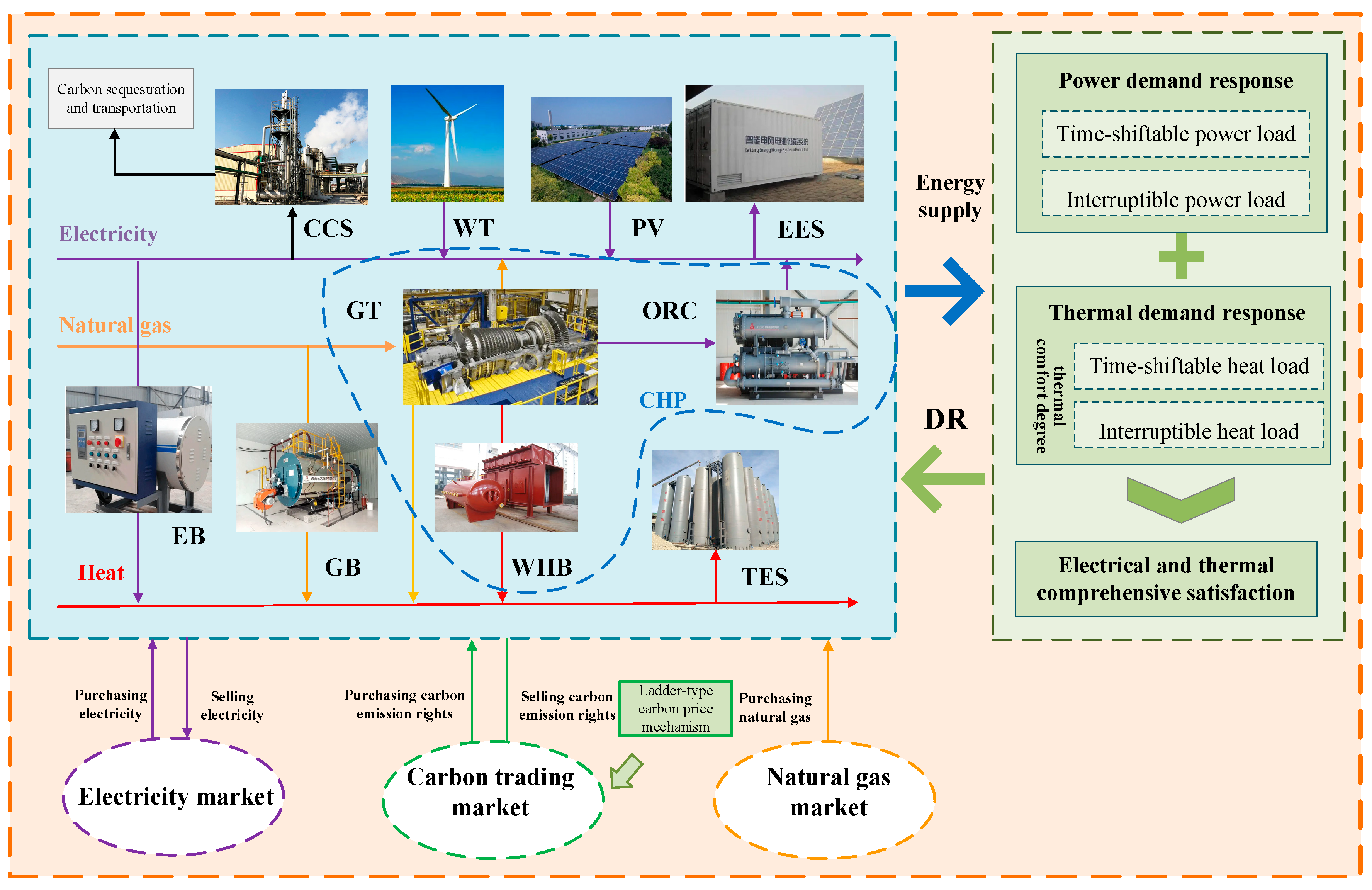
The VPP set up in this study consisted of controllable units (GT, ORC-WHB, EB, GB), uncontrollable units (distributed wind turbines, distributed PV generators), energy storage (EES, TES), and user loads (electric and thermal loads). The electric load in the VPP was supplied by GT, EES, ORC, WT, and PV; the thermal load was supplied by WHB, EB, GB, and TES.
Figure 1 shows the proposed VPP architecture. The blue box is the energy supply part of the VPP, which provides electricity and heat to meet the multiple energy demands of users through the joint operation of multiple energy devices. The green box is the energy use part, which not only uses the energy from the supply part but also aggregates the user’s power and heat IDR resources. The load-side user actively responds to its multi-energy demand and reduces or shifts a certain amount of load through incentive signals to ensure user satisfaction with energy use to achieve peak shaving and valley filling of the system. Notably, the CCS and EB operation requires electric energy input, and they are also considered as a special class of loads that can be engaged in carbon capture and electric to thermal conversion, respectively, while participating in power DR according to the energy supply and demand situation of the system at each time.

Figure 1.
VPP architecture.
During operation, the VPP generates power through internal new energy including WT and PV; CHP starts for power and heat co-generation, and GB and EB start for heat supply through energy conversion or purchase power from the external grid to meet the energy demand on the customer side. When the new energy generation output is in surplus or the electricity market price is low, VPPs can use EB to convert surplus electricity into heat, turn on the CO2 generated by the CCS, or use EES and TES to store the electricity and heat. In addition, the customer side can shift the demand from the peak load period to this time. When the new energy generation is not enough to supply the load or the electricity market price is high, CHP can be turned on, or the energy stored in EES and TES can be used to release electric or thermal energy. Users can cut and transfer the energy demand in this period.
2.1.2. Operation and Scheduling Mode of ELDR Mechanism
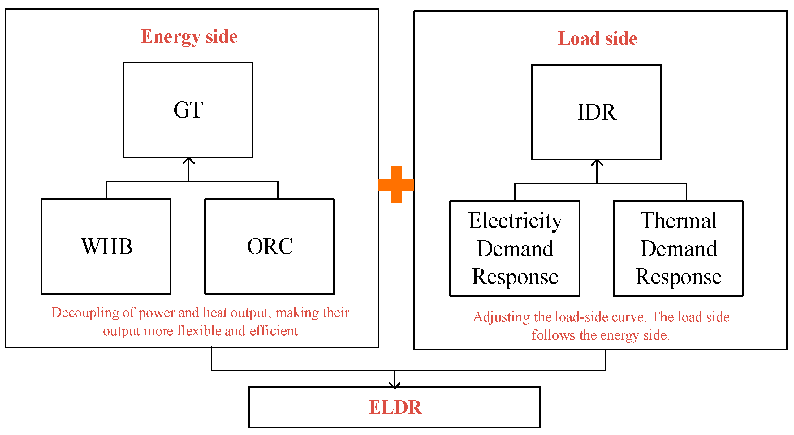
To promote renewable energy consumption, improve system energy efficiency, and realize low-carbon VPP operation, this study proposes a source-load dual response mechanism to realize reasonable allocation of energy output on the energy side and an energy consumption plan on the load side. This is achieved by coordinating the flexibility resources on both sides, improving the traditional way of participating in system regulation only through load-side demand response, enhancing the interaction ability of both sides, and improving the system operation flexibility and load-side power satisfaction.
Specifically, ORC-WHB is introduced on the energy side of the VPP to decouple the CHP “with heat to determine electricity” or “with electricity to determine heat” constraint. Simultaneously, the ORC-WHB is introduced on the load side to form a reasonable electricity consumption guide for customers through the electricity and heat IDRs to promote the transformation of energy consumption patterns, thereby reducing electricity consumption costs and further improving the energy efficiency of the VPP, as shown in Figure 2.
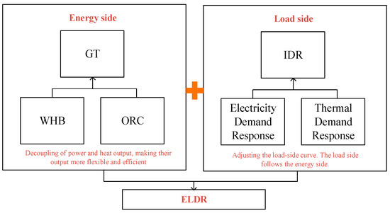
Figure 2.
ELDR.
The VPP scheduling process based on the ELDR mechanism can be described as follows.
(1) Controllable units such as GT, WHB, ORC, EB, and GB on the energy side must report the dispatchable output at each moment of the next day to the VPP operation and management organization through the day-ahead information declaration mechanism.
(2) Energy storage devices such as EES and TES are required to report charge and discharge capacity, charge status, and other related information at each moment of the next day.
(3) The VPP operation and management organization forecasts the load-side electric and thermal loads and their regulable potential. The CUS index on the load side is used to judge the degree of load DR.
(4) The VPP operation and management agency judges whether to allocate the response volume for each time period on the energy and load sides based on the following day’s new energy generation output forecast value, load-side electric and thermal load, adjustable potential forecast value, grid electricity price, carbon emission price, and other information based on the energy-side equipment operation cost and load CUS index. The supply side completes the task of reasonably allocating the hot flue gas emitted by GT to WHB and ORC according to the demand of the electric and thermal loads; the load-side electric and thermal loads complete the response to the output of supply-side equipment by changing the energy consumption plan through the DR that they can perform. The CCS completes the response to the electric load according to the remaining power in each time period.
2.2. Model Framework
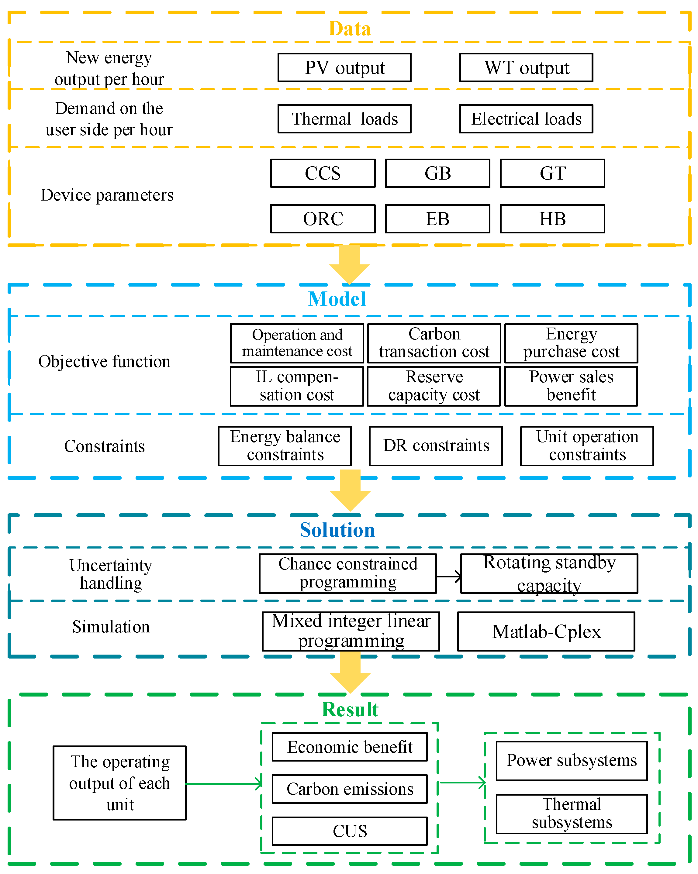
The uncertainty in the capacity of the WT, PV, and load demand units in VPPs may lead to failure to provide the corresponding capacity as planned, resulting in imbalance between supply and demand. In this study, the uncertainty of new energy output and load demand was solved by opportunity-constrained planning, and the confidence level α was introduced to guarantee system supply and demand balance within a certain probability α. The model framework of this study is shown in Figure 3.

Figure 3.
Model framework.
- Input the hourly output of WT and PV, the basic parameters of each device on the source side, the parameters related to the load demand response potential, and the electric and thermal load demand.
- Based on the CUS, the VPP low-carbon economic dispatch optimization model was constructed with the minimum total cost as the objective function, the operating conditions of each type of unit, the DR limits of each type of load, and the balance of energy supply and demand as the constraints, considering ELDR.
- Considering the uncertainty of WT, PV, and load demand, the uncertainty was transformed into certainty by the opportunity-constrained planning method.
- The VPP economic low-carbon dispatch optimization model was solved with ELDR using MATLAB 2019a, and the decision variables, such as the response quantity of each unit on the energy side and demand response quantity on the load side at each time, were solved.
- The ELDR system was operated and output the optimal total operating cost, carbon emission, and CUS.
3. VPP System Modeling
3.1. IDR Modeling
3.1.1. Electric Load Uncertainty Model
Electric load power fluctuations can be approximated as obeying a normal distribution [24], and in this paper, a normal distribution function is used to describe the electric load fluctuations, whose probability density function can be described as:
where is the active power of the load, and are the expected value and standard deviation of the probability density function of the electric load power, respectively.
3.1.2. Heat Load Modeling
Thermal load demand is related to indoor and outdoor temperature and building parameters, and indoor temperature is related to human comfort. The PMV index was introduced in this section to describe the acceptable comfort range of users, which can be expressed as:
where M is the energy metabolic rate of the human body, is the thermal resistance of the garment, is the average temperature of the human skin in a comfortable state, and is the room temperature. The recommended PMV index range according to the ISO7730 standard is [−0.5, 0.5].
Once the indoor temperature is determined, a link between the temperature and indoor heat load demand must be established. Previous studies have shown that the relationship between indoor temperature and heat load demand satisfies a first-order ordinary differential equation, which can be described as:
where and are the indoor and outdoor temperatures in period t, C and R are the equivalent heat capacity and equivalent heat resistance of the building, and is the initial heat load demand in period t.
3.2. IDR Modeling Based on RMM
Users can enter into agreements with VPP operators to participate in IDR, and they can increase the flexibility of virtual power plant operation by adjusting the energy consumption load. Electric and thermal loads can be divided into fixed loads, time-shiftable loads, and interruptible loads, where time-shiftable and interruptible loads can participate in IDR as adjustable loads.
3.2.1. User Participation in IDR Willingness Modeling
In the actual IDR dispatch of the VPP, for rational individual users, their choice to participate in IDR and their level of participation depends on the balance between the expected benefits they receive and the compensation gap after IDR. In general, a high benefit will increase the willingness to choose to participate in IDR, while a lower benefit will be a deterrent to participation. In the actual IDR dispatch of a VPP, for a rational individual user, the decision to participate in IDR and the degree of participation depend on balancing the expected benefits against the compensation gap after IDR. Generally, higher compensation incentivizes participation, while lower compensation deters it. A realistic strategy for users to maximize benefits may be to assess profitability by observing and learning from their previous IDR participation experience, which follows the behavioral “reflex-response” paradigm. In order to derive the degree of user participation in IDR at each time, this paper introduces an improved RMM to construct a behavioral probability model of user participation in IDR. IDR-participating users choose their next participation strategy (i.e., the degree of participation in IDR) based on the results of the combination of compensation and benefit loss from past participation in IDR.
(1) User Benefit Model
According to the RMM-based user willingness model, users’ willingness to participate in IDR depends mainly on its historical profitability and changes over time. Here, the user benefit is defined as the difference between the compensation they receive for participating in IDR and the benefit discount. The compensation of the interruptible load is linearly related to the size of the interruptible load, the compensation of the time-shiftable load is related to the maximum rated power of the time period, and the benefit discount of the interruptible load and time-shiftable load obeys quadratic and exponential functions, respectively, as shown in the following equations:
where is the benefit of user participation in IDR, , , , are the compensation obtained by the user’s time-shiftable electric load, interruptible electric load, time-shiftable thermal load, and interruptible thermal load after participating in the IDR project, respectively, and , , , are the corresponding benefit losses. , , , are the compensation rates for time-shiftable electric loads, interruptible electric loads, time-shiftable thermal loads, and interruptible thermal loads in the IDR program, respectively. , , , , , , , , are user utility parameters.
(2) Improved RMM
This section models the user’s willingness to participate in IDR based on RMM. Firstly, the user’s willingness degree to participate in IDR is discretized, i.e., , assuming that the value step of is 0.1 and the value range is [0, 1]. The user chooses the degree of participation in this IDR after receiving the IDR scheduling signal from the VPP operator, i.e., a policy is chosen. The regret degree measure for regretting not choosing policy but choosing policy in the nth IDR event can be expressed by the following equation.
where is the regret measure after the user chooses to select the switch of the current participation policy in the nth IDR event. h is the ordinal metric of the number of IDR calls.
and are the gain values when the user participates in the IDR invocation with policy and in the hth IDR event, respectively. If the user chooses to participate in the strategy in the nth IDR event, then the probability that the user chooses to switch to strategy in the th IDR event and still adheres to strategy can be expressed as:
where is the number of elements in the user’s strategy set, which is 11 here. is the inertia coefficient of the user’s adherence to the original strategy.
Based on the above model, when users select the IDR participation policy for the next phase, they will make a judgment based on the actual utility value of their own historical participation in IDR and the corresponding policy, from which they can derive the IDR resources that can be scheduled by users in a certain time period.
3.2.2. User IDR Volume Modeling
The time-shiftable loads and interruptible loads in the electric load need to participate in IDR within their responsiveness, which is modeled as follows: (1) Electric load DR modeling
where , are the time-shiftable and interruptible electric loads at time t. , are the maximum values of the time-shiftable electric loads; , are the maximum values of the interruptible loads. is the willingness to participate in the electric DR, assuming that their willingness to participate in time-shiftable and interruptible electric loads is equal. (2) In thermal load DR modeling, the heat load demand for each time period can be obtained through Equation (3). In addition, this section considers that the heat load has time-shiftable and interruptible characteristics, as follows:
where , are the time-shiftable and interruptible loads at time t; , are the maximum values of the time-shiftable loads; , are the maximum values of the interruptible loads; and is the customer’s willingness to participate in the thermal DR, assuming that their willingness to participate in time-shiftable and interruptible loads is equal.
Combined with the electric and thermal load model, the demand-side electric and thermal equivalent loads can be derived as:
where and are the equivalent electric and thermal load power, and , , and are the fixed, time-shiftable, and interruptible electric loads in period t, respectively.
To comprehensively measure the impact of the combined electric and thermal demand response on user comfort, a combined comprehensive user satisfaction (CUS) index was designed in this section and can be expressed as
3.3. New Energy Generation Unit Modeling
The WT and PV generation in VPPs has uncertainty and can be described by the probability density function. The WT output is related to the wind speed and its rated output, and the wind speed obeys the Weibull distribution [25]. The probability density function of WT output is expressed as follows:
where and are the scale and shape factors, respectively; is the rated output of WT; and are the cut-in and rated wind speeds, respectively.
PV output is related to solar radiation intensity and obeys gamma distribution [26], and its probability density function output is as follows:
where is the maximum value of PV unit output, and are scale coefficients, and is the gamma function.
To facilitate the treatment of multiple random variables, this paper introduces net electric load to represent the difference between WT and PV output and electric load demand.
3.4. Thermoelectric Coupling Units Modeling
3.4.1. CHP Model
- GT modelwhere , , and are the natural gas calorific value, GT power generation efficiency, and GT natural gas input in period t, respectively.
- 2.
- ORC modelwhere is the proportion factor of the hot flue gas emitted by GT absorbed by ORC, and and are the generation efficiency and power of ORC, respectively.
- 3.
- WHB model
Combining Equations (1)–(3), the CHP electric heat output power of the energy side can be expressed as:
where and are the CHP electric and thermal power outputs in period t.
3.4.2. EB Model
3.5. CCS Modeling
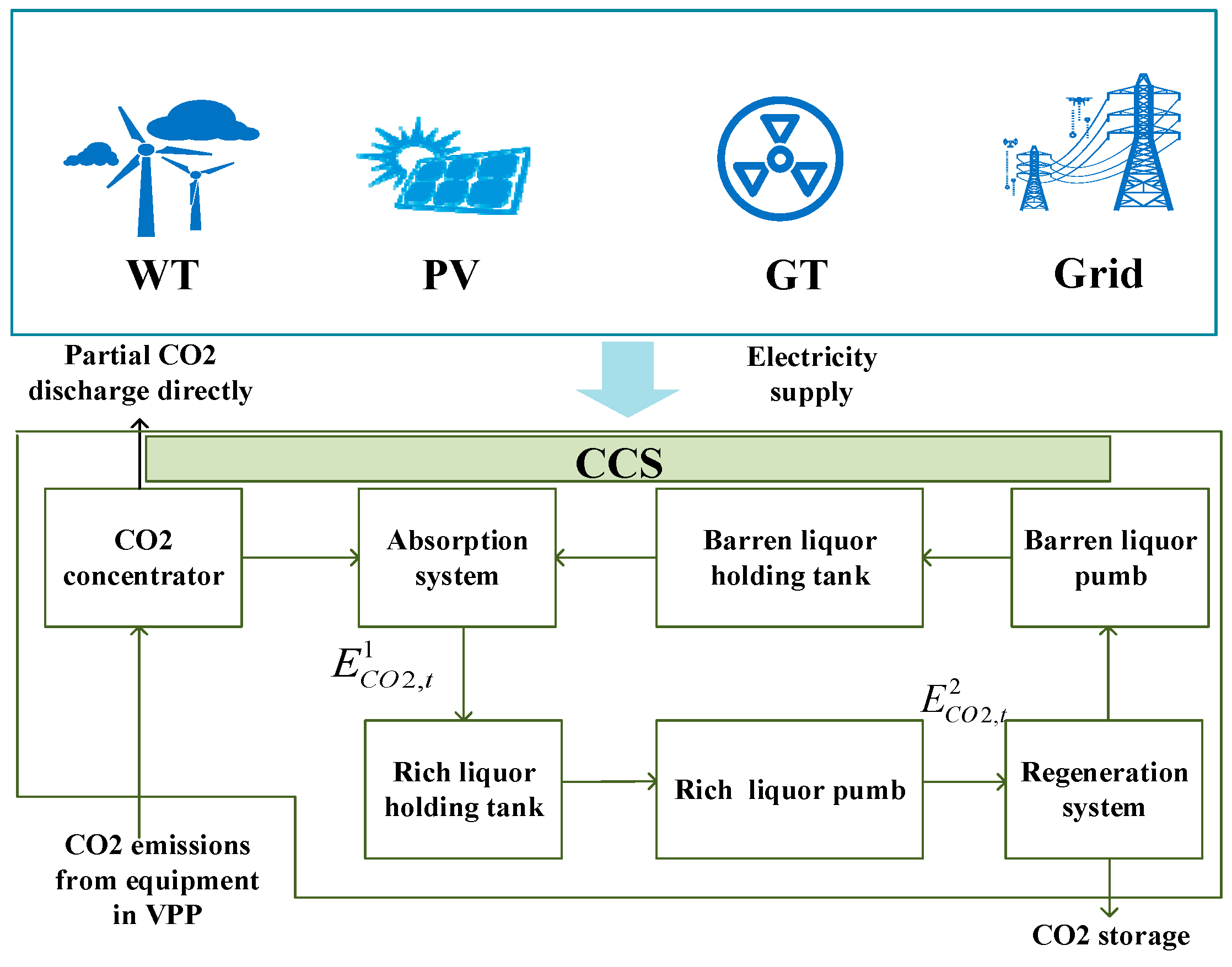
This study adopted the post-capture method to absorb the CO2 emitted by the VPP, and the electricity for CCS operation was supplied through the coordination of new energy and GT generation and the low-valley electricity of the large power grid; the specific operation process of the CCS is shown in Figure 4.

Figure 4.
Carbon capture schematic.
The CO2 emitted from the CHP and GB in the VPP during operation can enter the CCS through the CO2 concentrator. Unlike the carbon capture retrofitted thermal power plant, in the carbon capture operation mode proposed here, the CCS uses the surplus power inside the whole VPP for carbon capture, so that the new energy in the VPP can be fully utilized.
The CCS requires an external power supply for CO2 capture, and the specific model is as follows:
where is the energy consumption per unit CO2 treated by the CCS regeneration system, is the CO2 capture rate of the CCS, is the fixed energy consumption of the CCS, and is the energy consumption of CCS operation. is the amount of CO2 entering the rich liquor holding tank, and is the amount of CO2 treated by the CCS.
The configuration of rich and barren liquor holding tanks in the CCS plant can decouple the CO2 absorption and regeneration processes and enhance the flexibility of the carbon capture plant. The specific model is as follows:
where and are the CO2 storage volumes of the rich and barren liquor holding tanks in period t, and are the volumes of liquor flowing into and out of the rich liquor holding tank, and and are the volumes of liquor flowing into and out of the barren liquor holding tank. According to the operation of the CCS, the flow volumes of the inlet and outlet rich and barren liquor satisfy the following conditions.
One unit of rich liquid can absorb 25 units of CO2:
3.6. GB Modeling
3.7. Energy Storage Device Modeling
Energy storage devices are divided into electric and thermal energy storage. The specific models are as follows:
where is the capacity of the nth energy storage in period t, and is the self-loss rate of the nth energy storage. n = e for electric energy and n = h for thermal energy storage. and denote the nth energy storage charging and discharging power in period t, respectively. and are the nth energy storage charging and discharging power in period t. and are the nth energy storage charging and discharging efficiency, and is the scheduling time.
4. VPP Operation Optimization Model
4.1. Objective Function
We constructed an objective function to minimize the total cost of the VPP, considering energy purchase cost , carbon trading cost , carbon sequestration and transportation cost , O&M cost , rotating backup cost , interruptible load compensation cost , and system power sales efficiency :
4.1.1. Energy Purchase Cost
4.1.2. Carbon Trading Cost
To control the total carbon emission of the VPP and stimulate its carbon emission potential, we adopted a ladder-type carbon price mechanism to calculate the carbon emission cost of the system. The CHP and GB in the VPP proposed in this study generate carbon emissions, and when the actual carbon emission of the VPP is higher than the quota allocated by the government, carbon emission allowances must be purchased to compensate for the excess carbon emission. Different excess emissions correspond to different carbon prices, and the larger the excess emissions are, the higher the carbon price is. The actual carbon emission of the system is calculated as shown in Equation (23):
where is the total carbon emission of the VPP; and are the carbon emission coefficients of CHP and heat generation, respectively; and and are the carbon emission coefficients of GB and power purchase from a large grid, respectively.
China’s carbon trading market is still in the early stage, carbon emission allowances are allocated to the units used for carbon trading free of charge, and the benchmark value method is used to set corresponding carbon emission benchmark values for different categories of units. The VPP carbon allowances are calculated as follows:
where is the total amount of the VPP carbon quota; and are the carbon quotas of the CHP unit power and heat generation, respectively; and is the carbon allowance for the GB unit of energy supply.
Thus, the quotas to be purchased by the VPP are:
The system ladder-type carbon trading cost is calculated as follows:
where is the cost of VPP carbon trading, is the base price of carbon trading, is the carbon price growth coefficient, and h is the length of the carbon emission interval.
4.1.3. Carbon Sequestration and Transportation Cost
4.1.4. Operation and Maintenance Cost
4.1.5. Rotating Backup Cost
Rotating standby can reduce the uncertainty of new energy unit output in the VPP, and we considered setting GT and EES as rotating standby equipment in the VPP to ensure the reliability of the VPP energy supply under a certain confidence level.
where and are the unit rotating standby cost coefficients of GT and EES, respectively, and and are the gas turbine and electric energy storage standby capacities in period t, respectively.
4.1.6. Interruptible Load Compensation Cost
4.1.7. System Power Sales Efficiency
4.2. Constraints
The constraints mainly include power balance, unit climbing, unit output, DR, CCS, energy storage equipment, and rotating standby operational boundaries. Among them, the DR-related constraints are described in Section 3.2.2. Other constraints are as follows.
4.2.1. Power Balance Constraints
4.2.2. Unit Climbing Constraints
The GT, ORC, WHB, EB, and GB units are also required to meet the climbing limit constraint:
where is the climbing power limit of the th unit.
4.2.3. Unit Output Constraints
The output of GT, ORC, WHB, EB, GB, and other units must meet their output limit constraints:
where is the output value of the th unit, and and are the upper and lower limits of the output of the first unit in period t.
4.2.4. CCS-Related Constraints
4.2.5. Energy Storage Equipment Constraints
4.2.6. Rotating Standby Constraints
The standby of GT should satisfy the constraint:
For EES, its standby shall satisfy the constraint:
where is the time slot length.
where is the expected value of the net electric load, and is the pre-set confidence level of the rotating standby.
5. Solution Method Based on Chance-Constrained Planning
For optimization models containing uncertain constraints, chance-constrained planning is an effective way to solve them. Chance-constrained planning was proposed by Charnes and Cooper [27], and its main principle is to use probabilistic constraints to describe uncertain constraints to seek the optimal solution of the model. The output of WT and PV units in this study was constructed as random variables. We used chance-constrained planning to describe the uncertainty of WT and PV output in the model and generate probabilistic sequences according to the cumulative probability distribution of WT and PV output and used convolution calculations to form probabilistic sequences of common outputs, so that the chance constraint was transformed into a deterministic constraint. The general form of the chance-constrained planning can be expressed as:
where is the objective function, is the random parameter vector, is the constraint, and is the probability of the event holding. and are the pre-given confidence levels. is the traditional deterministic constraint; is the minimum value of the objective function at a probability level no lower than .
(1) Probabilistic serialization of random variables
The output of WT and PV units in period t is a random variable, and the corresponding probabilistic sequences and can be obtained from their probability distributions, which are a discretization of the probability distribution of the WT and PV unit output continuity. The length of the probabilistic sequence of the PV output is:
where is the maximum integer not exceeding , is the maximum PV output in period t, and is the discretization step, and owing to the rounding of the sequence length, there is a certain probability remaining when , which is included in . The PV output and its corresponding probabilistic sequence are shown in Table 1.

Table 1.
PV output and its probabilistic sequence.
The expected value of the probabilistic series is:
According to the WT and PV probability distribution, to calculate the common output of the two, we can obtain their probabilistic sequences and . Their sequence lengths are defined as and , respectively, and the calculation process is as follows:
The probabilistic series of WT, PV, and the electric load power with the discretization compensation of q for each time period can be obtained by Equations (57) and (58). And their power expectation for each time period can be calculated by Equation (56), where the net electric load power expectation is:
The WT, PV joint out power probabilistic sequence has sequence length , and its sequence probability can be calculated as follows:
Let the probability of the electric load sequence in time period t be ; the length of the sequence is , and the probability of the net electric load sequence in time period t can be calculated from and by the following equation.
Table 2 shows the correspondence between the probabilistic sequence of the net electric load power and the step size and length :
Table 2.
Net electric load output and its corresponding probability sequence.
Equation (53) contains , , and , three random variables with different distributions. To transform Equation (53) into the equivalence class of deterministic constraints, we must find the distribution of the random variable . To facilitate the description, we introduce the variable . The probability distribution of can be described as:
In this paper, is the probability density of the WT and PV outputs, respectively; is the probability density function of the load demand; and is the maximum value of electric load power. They can be obtained by inverse transformation, thus transforming the chance constraint into a deterministic constraint. However, because the function form is complex, difficult to find, and may not be unique, it usually needs to be processed by means of stochastic simulation. In this study, we used the theory of sequential operations to discretize the probability distribution of random variables to achieve the conversion of the deterministic constraint.
Here, the 0–1 variable is defined as:
Combining with Table 2, (53) can be transformed into
By transforming the chance constraint into a deterministic constraint through Equation (64), not only is the influence brought by the uncertainty factor in the operation of the VPP solved, but the drawbacks of the traditional chance-constraint solution can also be avoided.
(3) Constraint linearization
where is a large positive number. Equation (65) is equivalent to (64), and the linearization of Equation (53) is realized by Equations (64) and (65). As a result, the optimization model constructed in this study is transformed into a mixed-integer linear programming solvable form.
6. Example Analysis
6.1. Basic Data
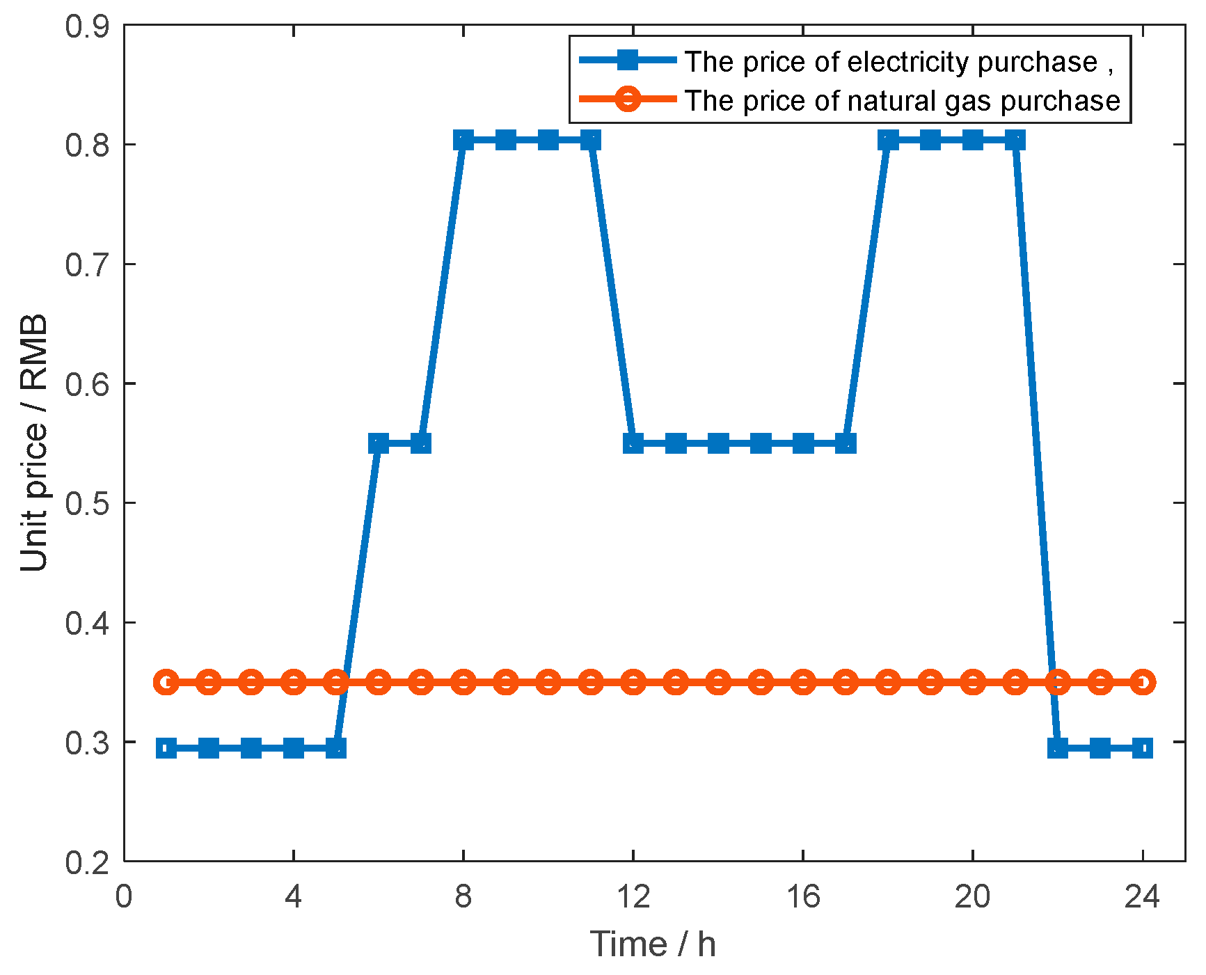
To verify the validity of the model proposed in this study, we selected a VPP demonstration project in North China as an arithmetic example for analysis. The key equipment of this VPP is shown in Figure 1, including WT, PV, EES, GT, EB, ORC-WHB, GB, TES, and other equipment. The WT and PV power output and electric and thermal load demands, system electricity purchase/sale price, and gas purchase price are shown in Figure 5 and Figure 6 [24,28,29]. The parameters of each operating equipment are shown in Table 3, Table 4 and Table 5. All generating units are from a virtual power plant located in North China.
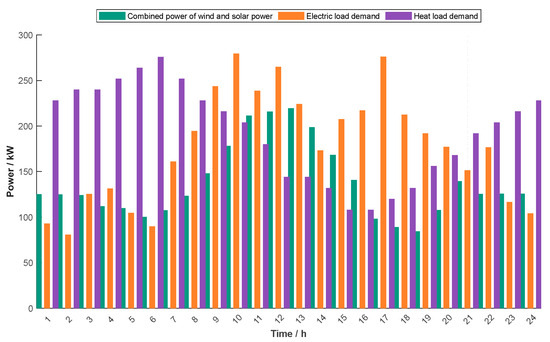
Figure 5.
Selected typical electric and thermal loads and combined WT and PV output curves.
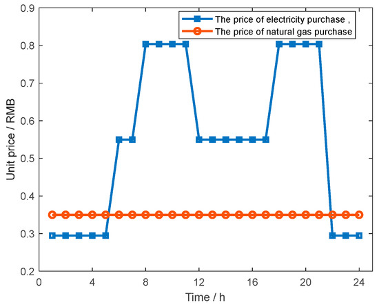
Figure 6.
Electricity purchase/sale price, gas purchase price.
Table 3.
Electrical- and thermal-related equipment parameters.
Table 4.
Energy storage parameters.
Table 5.
Other parameters.
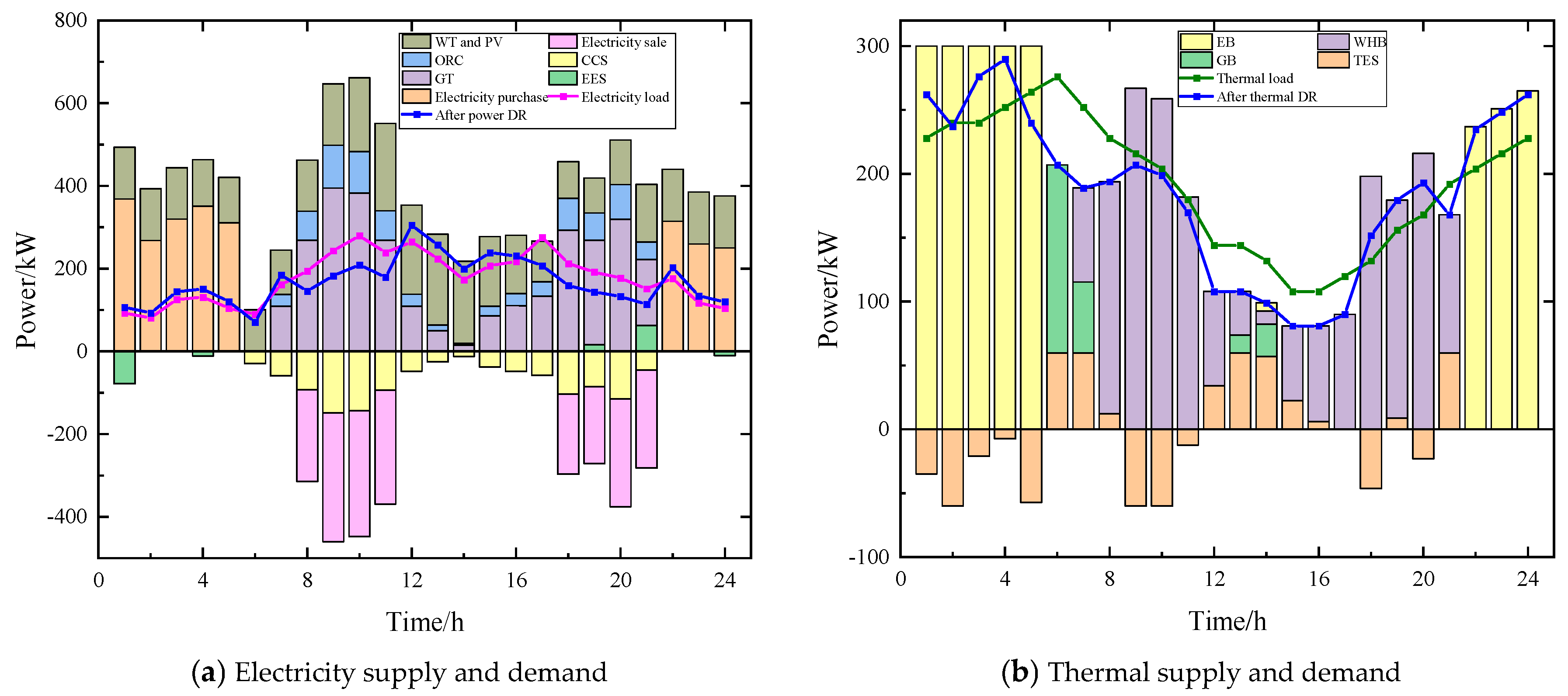
6.2. Optimized Scheduling Scheme Based on the ELDR Mechanism
The optimal operation scheme of the VPP under the ELDR is shown in Figure 7. At night (0:00–5:00, 22:00–24:00 h), the system electric and thermal loads were supplied by new energy and purchased electricity, and EES and TES stored part of the electricity and thermal power, while CHP and GB did not produce power. This is due to the new energy output being greater than the user’s electric load at this time, with a lower power purchase price and more abundant power. Therefore, the system can supply all the heat to the user through the electric heat transfer device EB in addition to supplying the user’s electric power and storing part of it. Because GT and GB are not turned on at night, the system does not produce carbon emissions; so, the CCS is shut down at night.
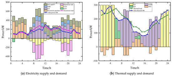
Figure 7.
Optimized operation scheme of VPP under ELDR.
From 6:00 to 22:00, GT supplied most of the electricity and heat load, GB supplemented the remaining heat load, and the CCS was turned on. This is due to the high demand for electricity and heat on the customer side during this period. Although the new energy output was higher during this period compared to the nighttime, it could not meet the full load demand and CHP was activated for power and heat co-generation. Because the electricity price was high and the power supply was tight at this time, most of the heat was provided by WHB absorbing the waste heat from GT generation, and the remaining part was made up by GB. As the GT and GB were turned on, the system carbon emission increased, and the CCS used the system to coordinate the dispatch of power for carbon capture.
In addition, the demand response performed by the customer side shifted the power from the peak to the low period, which made the load curve smooth considering the overall system cost and CUS constraints. Notably, during the hours of 8:00–11:00 and 19:00–21:00, the VPP sells surplus power to the larger grid for power sales revenue by coordinating source- and load-side resources according to the tariff of the corresponding hours.
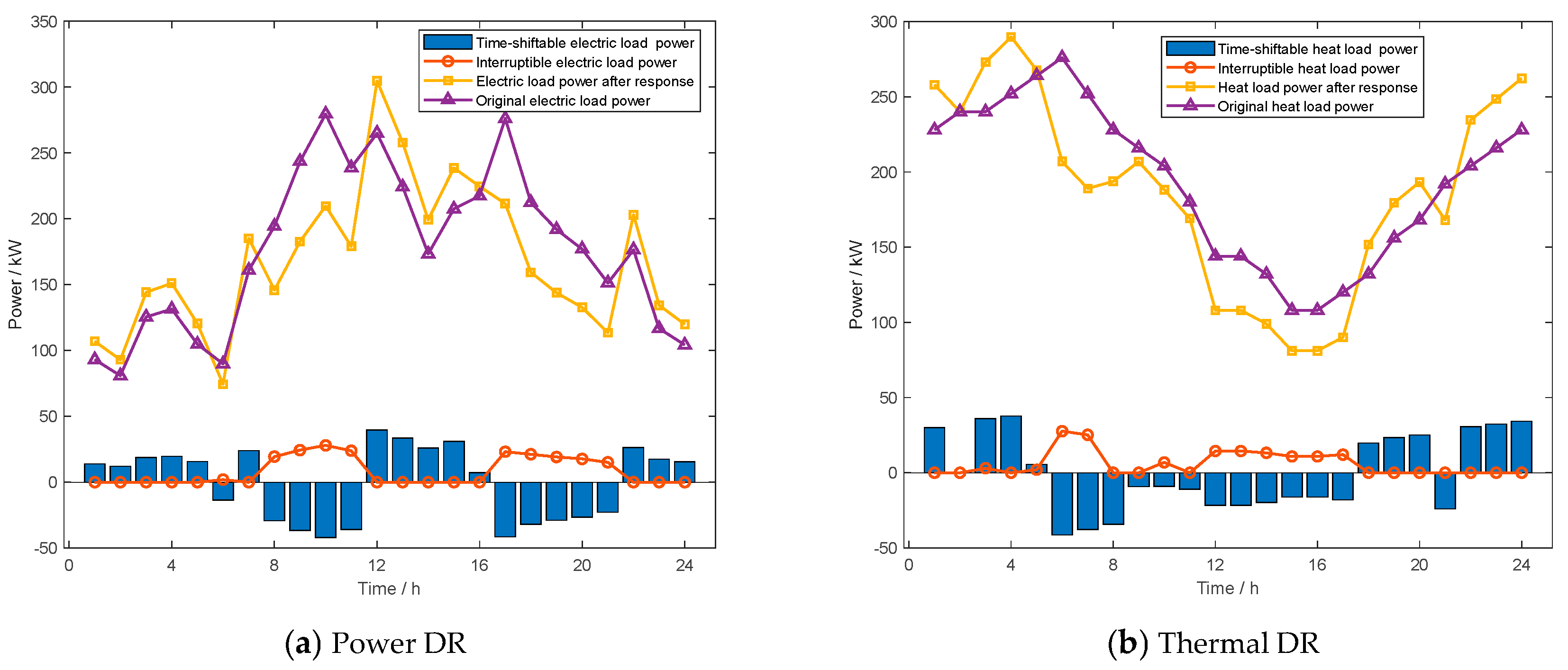
Figure 8 shows the effect of specific load-side demand response. In terms of electricity demand response, the customers shifted the electric load from the peak of the 8:00–11:00 and 17:00–21:00 h periods to the low hours of electricity consumption (0:00–5:00, 12:00–16:00, and 22:00–24:00). Additionally, because of the peak hours when the electric load is higher, there is electricity supply tension, but also a certain amount of electric load interruption to ensure that the system supply and demand are balanced. In terms of thermal demand response, the customers shifted the thermal load from the 6:00–17:00 h to 0:00–4:00 and 18:00–24:00 periods, and a certain number of interruptions were made to the thermal load from 5:00 to 7:00 and 12:00 to 17:00. This is because most of the thermal load was supplied by the waste heat of the GT absorbed by the WHB, while the electric load was at a higher level, and the system sold electricity to the grid with little effect on the overall economic efficiency. To ensure the economy of the system, most of its electric load was supplied by new energy sources, and the GT output was low, which can only meet the basic heat load, and it must be interrupted to some extent.

Figure 8.
Effect of specific load-side demand response.
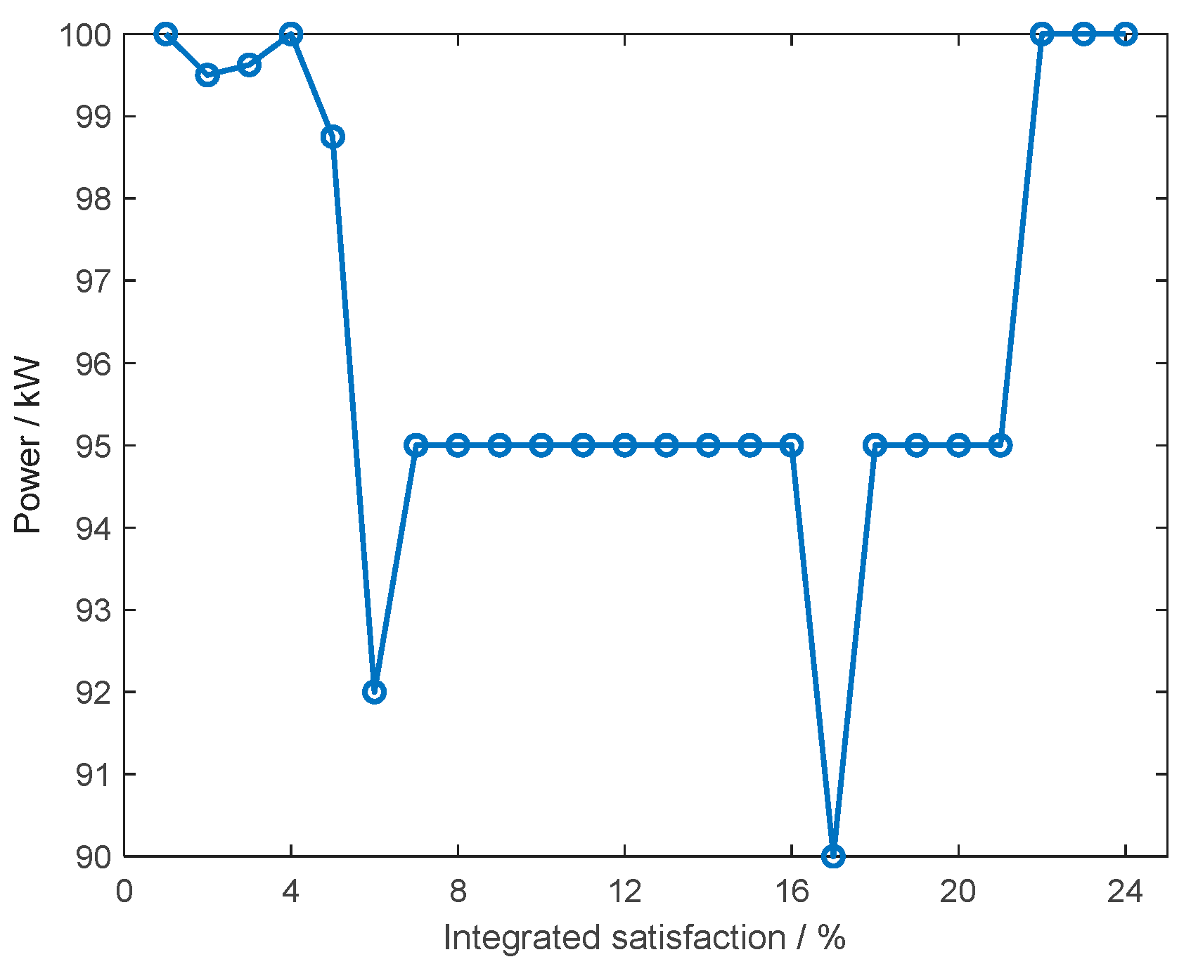
Figure 9 shows the CUS at each time period. Figure 7 and Figure 8 show that the CUS was highest from 0:00 to 4:00 and 22:00 to 24:00 due to sufficient energy supply. However, from 5:00 to 21:00, the CUS level decreased because the system must provide demand response for load interruptions, but the CUS level remained above 90%, which is within the acceptable range of users.
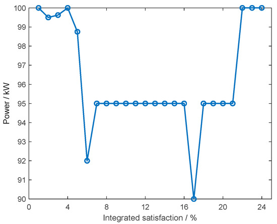
Figure 9.
The CS under ELDR.
6.2.1. Results Analysis Comparison of Operation Scenarios of VPP Optimization
To verify the validity of ELDR, the following four scenarios were set up for comparative analysis.
Scenario 1: without considering ORC-WHB and IDR.
Scenario 2: considering ORC-WHB but not IDR.
Scenario 3: considering IDR but not ORC-WHB.
Scenario 4: Considering both ORC-WHB and IDR.
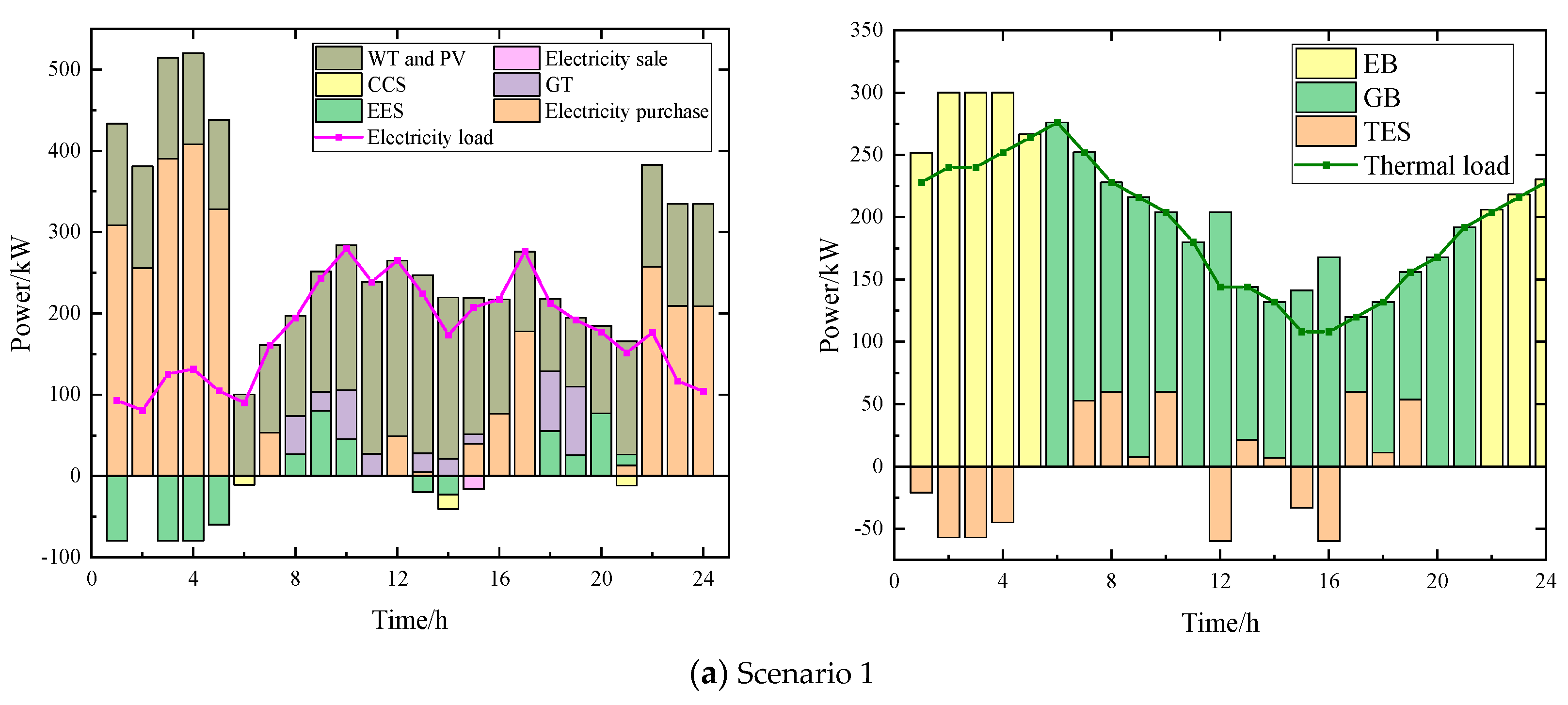
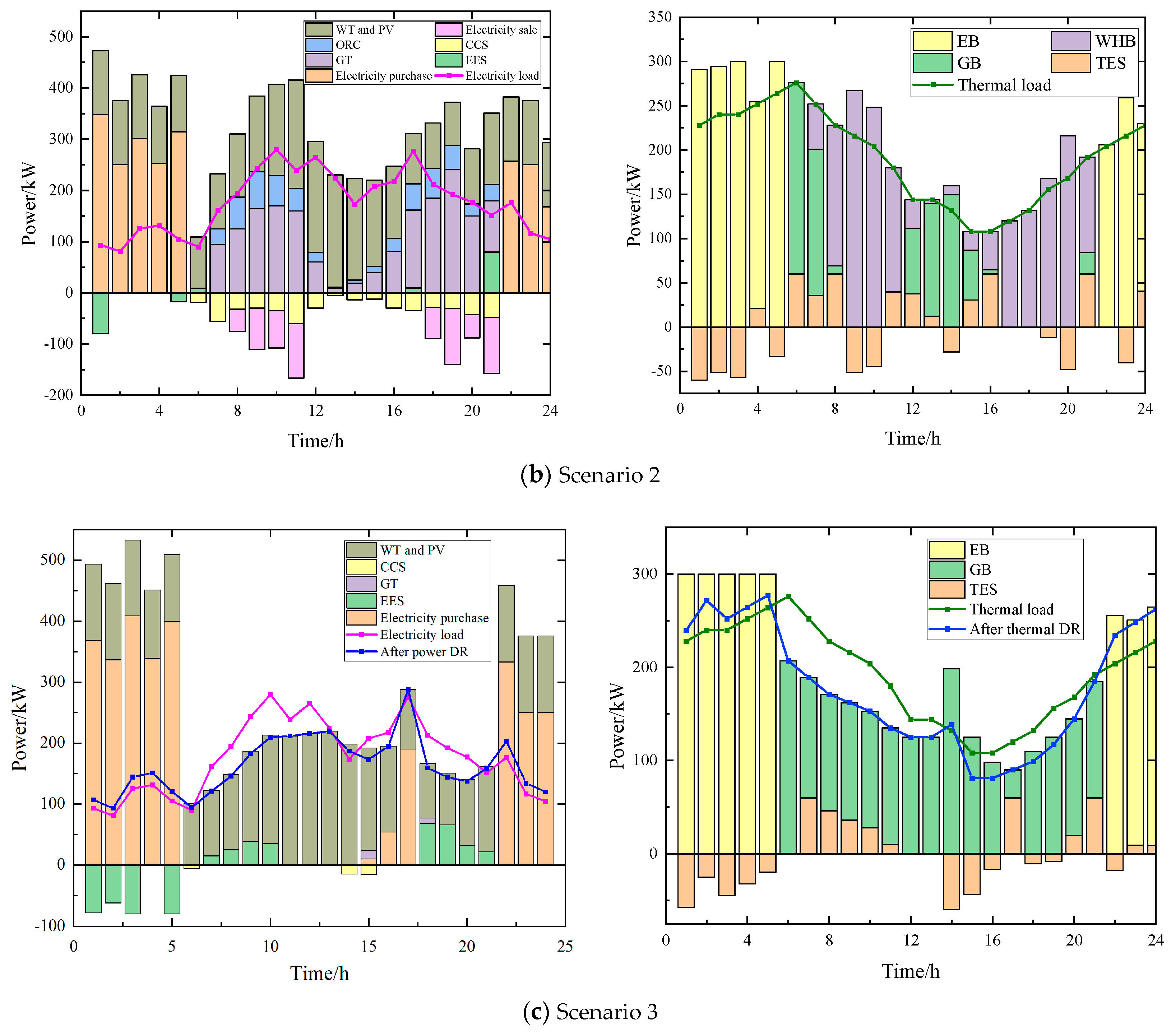
The optimized scheduling results for each scenario are shown in Table 6 and Figure 9. The result diagram of Scenario 4 is shown in Figure 6.
Table 6.
Optimized scheduling results for each scenario.
Comparing Scenarios 1 and 2, from an economic point of view, Scenario 2 had a 42.42% reduction in total cost compared to Scenario 1, which means that the configuration of ORC-WHB can improve the system economy. Scenario 2 reduced the energy purchase cost by 60.6% compared to Scenario 1, which is due to the introduction of ORC-WHB on the energy side of the VPP, which reduces the energy loss and thus reduces the energy purchase cost of the VPP from external sources. Figure 10a,b show that the deployment of ORC-WHB on the energy side can improve the energy supply efficiency of the system during the peak load hours of 6:00–21:00, which not only eliminates the need to purchase power from the grid but also allows the use of surplus power for carbon capture and sales to the larger grid for revenue while ensuring customer load. However, owing to the introduction of ORC-WHB, two types of equipment for the flexible regulation of electric heat, more O&M costs were incurred, increasing by 28.71% in Scenario 2 compared to Scenario 1. From the perspective of environmental protection, the carbon emission of Scenario 2 decreased significantly compared with Scenario 1, reducing 659.37 kgCO2 of emissions. This indicates that by coordinating the electric and thermal output of the energy side through the configuration of ORC-WHB, more surplus power can be coordinated to supply the CCS for carbon capture. Combined with Figure 10a,b, the operating hours and total operating power of the CCS in Scenario 2 increased, which can reduce the carbon emission of the VPP to a greater extent. Thus, the ORC-WHB waste heat recovery device can improve the environmental benefits while ensuring the system economy.

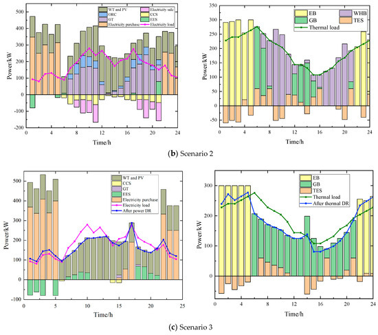
Figure 10.
Scenarios 1, 2, and 3 scheduling optimization results.
Comparing Scenarios 1 and 3, from an economic point of view, the total cost of Scenario 3 was reduced by 3.46%. In particular, the energy purchase and O&M costs of Scenario 3 were reduced by 3.47% and 64.72%, respectively. This is because Scenario 3 reduced the demand for heat and electricity during the 6:00–21:00 h period and increased the demand for heat and electricity from 0:00 to 5:00 and 22:00 to 24:00 through IDR, with adjustable load shifting and interruptions, thus achieving peak cutting and valley filling. From the perspective of environmental friendliness, the carbon emission of Scenario 3 was only 315.78 kg less than that of Scenario 1. This is due to the lower energy efficiency of the GT without the waste heat device. Combined with Figure 10c, we find that in Scenario 3 the GT was barely activated and relied mainly on demand response to match the power output, and the power supply only met the power demand of customers, while the heat load was mainly supplied through the GB. Hence, less surplus power was available for the CCS to use, resulting in less CO2 absorption from the GB. Interestingly, comparing Scenarios 3 and 2, the total cost of Scenario 3 was 68.44% higher, indicating that the implementation of IDR has some economic benefits, but its benefits are not as good as the configuration of waste heat recovery units on the energy side.
Scenario 4, which considers both the energy-side waste heat recovery unit and load-side IDR, had the lowest cost among the four scenarios, and its overall economic efficiency was the best. In particular, the total cost was reduced by 27.46% compared to Scenario 1. In terms of environmental friendliness, ELDR can more efficiently use the surplus energy at each moment for carbon capture or sale for profit. The carbon emissions were reduced by 736.09 kg compared to Scenario 1. Furthermore, both energy- and load-side responses can reduce the demand for load DR by coordinating the energy-side output compared to IDR only. Therefore, the average CUS of Scenario 4 increased by 3.75% compared to Scenario 3. This shows that ELDR had the best overall benefit, which can improve the system economy and environmental protection while ensuring the energy comfort of customers.
6.2.2. Sensitivity Analysis of New Energy and CCS Installed Capacity
The installed capacity of wind and PV units affects the output of each VPP unit and its overall operating benefit. In this section, a sensitivity analysis is conducted for the installed capacity of new energy and the CCS, as shown in Figure 10 and Figure 11:
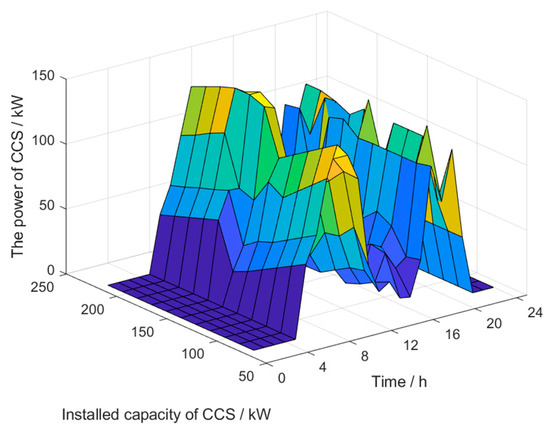
Figure 11.
Relationship between installed capacity of new energy, time, and power of carbon capture equipment.
The following is a sensitivity analysis of the installed capacity of new energy and CCS, respectively.
(1) Sensitivity analysis of new energy installed capacity
Figure 11 shows the effect of the change in the installed capacity of new energy on the distribution of the system carbon capture operation time. The change in the installed capacity of new energy affects the magnitude of the system carbon capture operation power, but the effect on the distribution of its operation time is not significant. The higher the installed capacity of new energy sources is, the more surplus power the VPP can coordinate for the CCS operation, resulting in higher capture power at each time. In terms of CCS carbon capture operation hours, the CCS was shut down during the 0:00–5:00 and 22:00–24:00 h periods because GT and GB were not turned on. From 6:00 to 21:00, the CCS operation was related to the GT output, with a higher GT output resulting in higher carbon emissions and relatively more remaining power available for the CCS operation. Therefore, the power of the CCS operation tended to increase from 5:00 to 10:00 and then decrease in the period from 11:00 to 14:00, gradually increase from 15:00 to 20:00, and decrease in the period from 21:00 to 24:00.
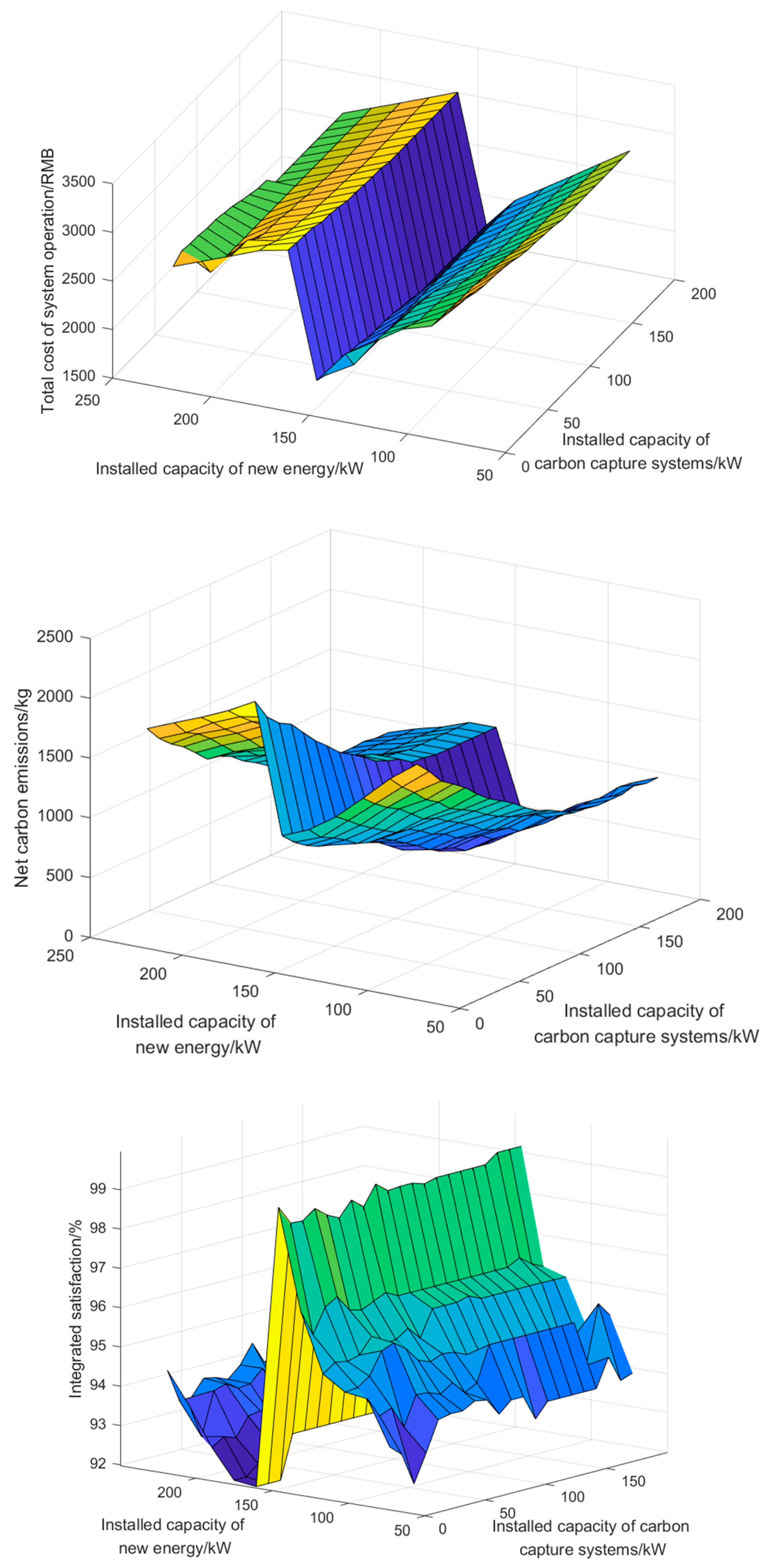
Figure 12 shows that the total system operation cost and carbon emissions exhibited a decreasing, then increasing, then decreasing trend as the installed capacity of new energy grew, while the CUS showed the opposite trend. Specifically, as the installed capacity of the new energy grew from 73 kW to 146 kW, the total system operating cost and carbon emissions decreased, while the CUS increased. This is because as the installed capacity of new energy in the VPP increased, the proportion of customer load during the peak hours of new energy supply gradually increased, so that the output of GT and GB units and the resulting O&M costs and carbon emissions decreased. Additionally, as the installed capacity of new energy increased, energy became increasingly abundant, and the system dispatched less power and heat for demand response on the customer side, causing the CUS to increase.
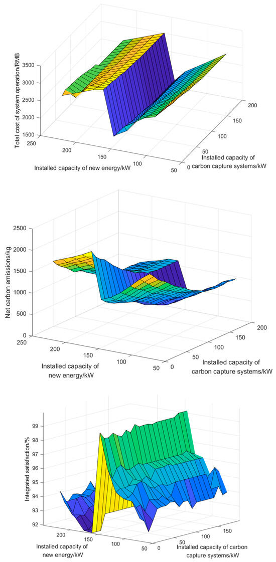
Figure 12.
Sensitivity analysis of carbon capture equipment capacity and CCS installed capacity.
As the installed capacity of new energy grew from 146 kW to 160 kW, the system operating cost and carbon emissions gradually increased and peaked, and the CUS gradually decreased. This is due to the unstable power output of the new energy sources, and as the installed capacity of the new energy sources continues to grow, a larger capacity for rotating backup must be allocated. The electric storage capacity is partially allocated as rotating backup, which cannot store the power during the energy surplus period and may lead to an increase in the output of GT, GB, and other units. In addition, the user side cooperates to provide demand response to alleviate the uncertainty caused by new energy output; so, with the further increase in new energy installed capacity, the VPP operating costs and carbon emissions continue to rise, and the CUS continues to decrease.
When the installed capacity of new energy continues to grow, the total operating costs and carbon emissions tend to decrease while the CUS slowly increases. This is because as the installed capacity of new energy continues to increase, the energy supply on the energy side becomes sufficient to meet the energy demand of the customer side at all times, and the surplus power outside the supply load is directly put on the grid, allowing the revenue from the sale of electricity to keep increasing.
The total installed capacity of the new energy in the example in Section 6.2 was 146 kW. Overall, the current installed capacity of new energy is in a better state with the same capacity configuration of other equipment in the system. To further increase the installed capacity of new energy in the future and improve the system’s new energy consumption, we must consider introducing more customer loads and the configuration of other equipment, such as GT, EES, and TES.
(2) Sensitivity analysis of the installed capacity of CCS
Figure 12 shows that the change in carbon capture equipment capacity affects the system carbon emissions. When the capacity of the carbon capture equipment grew from 0 kW to 120 kW, the net system carbon emissions kept decreasing because the CCS can absorb system carbon emissions. However, because of the limited effect of the CCS on system carbon emissions and energy coordination, the system carbon emissions remained stable as the CCS capacity grew to 120 kW.
In terms of total operating cost and CUS, no significant change was observed in total system cost and CUS with the change in CCS capacity. Thus, the system configuration of CCS can improve its environmental benefits without affecting the CUS and the economic benefits of the system.
7. Conclusions
This study constructs an integrated optimization framework for the VPP incorporating carbon capture systems under the ELDR mechanism, with a particular focus on the synergistic optimization of economic efficiency, environmental performance, and user comfort CUS. Through comprehensive scenario analysis, the proposed model demonstrates substantial potential in balancing operational costs, carbon mitigation, and energy flexibility. The implementation of ORC-WHB units effectively decouples CHP generation, achieving 27.46% cost reduction and 45.28% emission reduction through peak shaving and waste heat recovery. The CCS technology exhibits time-dependent operational characteristics, primarily engaging during peak demand periods to offset CHP-related emissions while maintaining economic viability.
Despite the valuable insights provided by the current model under stationary operational conditions, several critical research avenues warrant exploration. First, while the marginal emission reduction benefits of the CCS plateau beyond a 120 kW capacity in our case study, and system economic/environmental performance deteriorates when renewable capacity exceeds optimal thresholds, future implementations must determine the optimal sizing of the CCS and renewable energy installations within VPPs to maximize overall system benefits. Second, detailed investigations into CCS performance across varied CHP operational regimes are essential, particularly regarding trade-offs between energy penalties and emission reduction targets. From a policy perspective, refined quantitative evaluations of interactions between carbon pricing mechanisms and ELDR incentives are needed to inform regulatory framework designs. Furthermore, advancements in predicting integrated demand response behaviors at the user level—through integration of machine learning techniques—could significantly enhance accuracy in forecasting electricity/heat demand responses under dynamic incentive structures. These extensions would not only enhance practical applicability but also contribute to developing more resilient and sustainable decentralized energy systems.
Author Contributions
Conceptualization, T.P. and Y.W.; methodology, T.P.; validation, Y.W.; formal analysis, Y.W.; investigation, T.P.; resources, Y.W.; data curation, R.C.; writing—original draft preparation, T.P.; writing—review and editing, Y.W. and R.C.; visualization, T.P. and Q.Z.; supervision, Q.Z.; project administration, Q.Z.; funding acquisition, Q.Z. All authors have read and agreed to the published version of the manuscript.
Funding
This work was financially supported by Demonstration of Transformation and Promotion for Integrated Development and Operation Methodology of Hydro-Wind-Solar-Storage Integration (Guizhou Science and Technology Cooperation Achievement [2025] General Project 001) and by the Fundamental Research Funds for the Central Universities (2025MS167).
Data Availability Statement
The original contributions presented in the study are included in the article; further inquiries can be directed to the corresponding author.
Conflicts of Interest
Author Ting Pan and Author Qiao Zhao were employed by Power China Guiyang Engineering Corporation Limited* during the study. The remaining authors (Yuqing Wang and Ruining Cai) declare that the research was conducted in the absence of any commercial or financial relationships that could be construed as a potential conflict of interest.
Abbreviations
| CCS | Carbon Capture System | GT | Gas Turbine |
| CHP | Combined Heat and Power | IDR | Integrated Demand Response |
| CUS | User Satisfaction | MILP | Mixed-Integer Linear Programming |
| DR | Demand Response | ORC | Organic Rankine Cycle |
| EB | Electric Boiler | RMM | Regret-Matching Mechanism |
| EES | Electric Energy Storage | TES | Thermal Energy Storage |
| ELDR | Energy-side and Load-side Dual Response Mechanism | VPP | Virtual Power Plant |
| GB | Gas Boiler | WHB | Waste Heat Boiler |
| VPP | Virtual Power Plan |
References
- Yang, Z.; Li, K.; Chen, J. Robust Scheduling of Virtual Power Plant with Power-to-Hydrogen Considering a Flexible Carbon Emission Mechanism. Electr. Power Syst. Res. 2024, 226, 109868. [Google Scholar] [CrossRef]
- Shi, T.; Qiu, X.; Tang, C.; Qu, L. Research on a Multi-Agent Cooperative Control Method of a Distributed Energy Storage System. Processes 2023, 11, 1149. [Google Scholar] [CrossRef]
- Hu, S.; Chen, Y.; Feng, J. A Flexible Interactive Coordination Control Method of Commercial Virtual Power Plant Based on WCVAR. Int. J. Electr. Power Energy Syst. 2024, 160, 110128. [Google Scholar] [CrossRef]
- Rouzbahani, H.M.; Karimipour, H.; Lei, L. A Review on Virtual Power Plant for Energy Management. Sustain. Energy Technol. Assess. 2021, 47, 101370. [Google Scholar] [CrossRef]
- Chai, T.; Liu, C.; Xu, Y.; Ding, M.; Li, M.; Yang, H.; Dou, X. Optimal Dispatching Strategy for Textile-Based Virtual Power Plants Participating in Grid Load Interactions Driven by Energy Price. Energies 2024, 17, 5142. [Google Scholar] [CrossRef]
- Tan, C.; Wang, J.; Geng, S.; Pu, S.; Tan, Z. Three-Level Market Optimization Model of Virtual Power Plant with Carbon Capture Equipment Considering Copula–CVaR Theory. Energy 2021, 237, 121620. [Google Scholar] [CrossRef]
- Chen, L.; Tang, H.; Wu, J.; Li, C.; Wang, Y. A Robust Optimization Framework for Energy Management of CCHP Users with Integrated Demand Response in Electricity Market. Int. J. Electr. Power Energy Syst. 2022, 141, 108181. [Google Scholar] [CrossRef]
- Mansour-Saatloo, A.; Agabalaye-Rahvar, A.; Mirzaei, M.A.; Mohammadi-Ivatloo, B.; Abapour, M.; Zare, K. Robust Scheduling of Hydrogen Based Smart Micro Energy Hub with Integrated Demand Response. J. Clean. Prod. 2020, 267, 122041. [Google Scholar] [CrossRef]
- Zeng, B.; Wu, G.; Wang, J.; Zhang, J.; Zeng, M. Impact of Behavior-Driven Demand Response on Supply Adequacy in Smart Distribution Systems. Appl. Energy 2017, 202, 125–137. [Google Scholar] [CrossRef]
- Waseem, M.; Lin, Z.; Liu, S.; Sajjad, I.; Aziz, T. Optimal GWCSO-Based Home Appliances Scheduling for Demand Response Considering End-Users Comfort. Electr. Power Syst. Res. 2020, 187, 106477. [Google Scholar] [CrossRef]
- Lu, Q.; Guo, Q.; Zeng, W. Optimization Scheduling of Integrated Energy Service System in Community: A Bi-Layer Optimization Model Considering Multi-Energy Demand Response and User Satisfaction. Energy 2022, 252, 124063. [Google Scholar] [CrossRef]
- Hadayeghparast, S.; Farsangi, A.S.N.; Shayanfar, H. Day-Ahead Stochastic Multi-Objective Economic/Emission Operational Scheduling of a Large Scale Virtual Power Plant. Energy 2019, 172, 630–646. [Google Scholar] [CrossRef]
- Yang, H.; Xiong, T.; Qiu, J.; Qiu, D.; Dong, Z.Y. Optimal Operation of DES/CCHP Based Regional Multi-Energy Prosumer with Demand Response. Appl. Energy 2016, 167, 353–365. [Google Scholar] [CrossRef]
- Basu, M. Optimal Day-Ahead Scheduling of Renewable Energy-Based Virtual Power Plant Considering Electrical, Thermal and Cooling Energy. J. Energy Storage 2023, 65, 107363. [Google Scholar] [CrossRef]
- Guo, X.; Wang, L.; Ren, D. Optimal Scheduling Model for Virtual Power Plant Combining Carbon Trading and Green Certificate Trading. Energy 2025, 318, 134750. [Google Scholar] [CrossRef]
- Laouid, Y.A.A.; Kezrane, C.; Lasbet, Y.; Pesyridis, A. Towards Improvement of Waste Heat Recovery Systems: A Multi-Objective Optimization of Different Organic Rankine Cycle Configurations. Int. J. Thermofluids 2021, 11, 100100. [Google Scholar] [CrossRef]
- Wang, H.; Hua, P.; Wu, X.; Zhang, R.; Granlund, K.; Li, J.; Zhu, Y.; Lahdelma, R.; Teppo, E.; Yu, L. Heat-Power Decoupling and Energy Saving of the CHP Unit with Heat Pump Based Waste Heat Recovery System. Energy 2022, 250, 123846. [Google Scholar] [CrossRef]
- Xi, H.; Zhu, M.; Lee, K.Y.; Wu, X. Multi-Timescale and Control-Perceptive Scheduling Approach for Flexible Operation of Power Plant-Carbon Capture System. Fuel 2023, 331, 125695. [Google Scholar] [CrossRef]
- Chen, X.; Wu, X. The Roles of Carbon Capture, Utilization and Storage in the Transition to a Low-Carbon Energy System Using a Stochastic Optimal Scheduling Approach. J. Clean. Prod. 2022, 366, 132860. [Google Scholar] [CrossRef]
- Li, J.; Zhang, C.; Davidson, M.R.; Lu, X. Assessing the Synergies of Flexibly-Operated Carbon Capture Power Plants with Variable Renewable Energy in Large-Scale Power Systems. Appl. Energy 2025, 377, 124459. [Google Scholar] [CrossRef]
- Wen, J.; Jia, R.; Cao, G.; Guo, Y.; Jiao, Y.; Li, W.; Li, P. Multi-Source Shared Operation Optimization Strategy for Multi-Virtual Power Plants Based on Distributionally Robust Chance Constraint. Energy 2025, 322, 135761. [Google Scholar] [CrossRef]
- Liu, X. Research on Bidding Strategy of Virtual Power Plant Considering Carbon-Electricity Integrated Market Mechanism. Int. J. Electr. Power Energy Syst. 2022, 137, 107891. [Google Scholar] [CrossRef]
- Du, Y.; Zhou, X.; Xu, T.; Tan, Z. Multi-Time Scale Cooperative Operation Optimization of Virtual Power Plant and Virtual Hydrogen Plant Under Stepped Carbon Trading Mechanism. Renew. Energy 2025, 248, 123104. [Google Scholar] [CrossRef]
- Li, Y.; Wang, B.; Yang, Z.; Li, J.; Li, G. Optimal Scheduling of Integrated Demand Response-Enabled Community-Integrated Energy Systems in Uncertain Environments. IEEE Trans. Ind. Appl. 2021, 58, 2640–2651. [Google Scholar] [CrossRef]
- Liang, C.; Ding, C.; Zuo, X.; Li, J.; Guo, Q. Capacity Configuration Optimization of Wind-Solar Combined Power Generation System Based on Improved Grasshopper Algorithm. Electr. Power Syst. Res. 2023, 225, 109770. [Google Scholar] [CrossRef]
- Wu, S.; Wang, Y.; Liu, L.; Yang, Z.; Cao, Q.; He, H.; Cao, Y. Two-Stage Distributionally Robust Optimal Operation of Rural Virtual Power Plants Considering Multi-Correlated Uncertainties. Int. J. Electr. Power Energy Syst. 2024, 161, 110173. [Google Scholar] [CrossRef]
- Charnes, A.; Cooper, W. Chance-constrained Programming. Int. J. Manag. Sci. 1959, 6, 73–79. [Google Scholar] [CrossRef]
- Li, Y.; Li, K.; Yang, Z.; Yu, Y.; Xu, R.; Yang, M. Stochastic Optimal Scheduling of Demand Response-Enabled Microgrids with Renewable Generations: An Analytical-Heuristic Approach. J. Clean. Prod. 2022, 330, 129840. [Google Scholar] [CrossRef]
- Wang, L.; Lin, J.; Dong, H.; Zeng, M.; Wang, Y. Optimal Dispatch of Integrated Energy System Considering Ladder-Type Carbon Trading. J. Syst. Simul. 2022, 34, 1393–1404. [Google Scholar]


Disclaimer/Publisher’s Note: The statements, opinions and data contained in all publications are solely those of the individual author(s) and contributor(s) and not of MDPI and/or the editor(s). MDPI and/or the editor(s) disclaim responsibility for any injury to people or property resulting from any ideas, methods, instructions or products referred to in the content. |
© 2025 by the authors. Licensee MDPI, Basel, Switzerland. This article is an open access article distributed under the terms and conditions of the Creative Commons Attribution (CC BY) license (https://creativecommons.org/licenses/by/4.0/).