Research on Industry–Economy–Energy–Carbon Emission Relationships Based on Panel Vector Autoregressive Modeling

Abstract

This study focused on the dynamic relationships among industrial development, energy consumption, economic growth, and carbon emissions in China, with the goal of achieving long-term ecological sustainability. Using the Panel Vector Autoregressive (PVAR) model and Generalized Method of Moments (GMM) estimation, panel data from 30 Chinese provinces between 2017 and 2021 were analyzed. The impulse response analysis and variance decomposition demonstrated that industrial and economic subsystems significantly influenced carbon emissions, while the energy subsystem had a moderating effect. These results highlight a shift in China’s energy consumption structure, with industrial and economic activities driving carbon emissions, while energy consumption patterns slowed the increase in emissions. These findings have critical implications for understanding the interactions among industry, economy, energy, and carbon emissions.

1. Introduction

With incremental improvements to its industrial system, China’s industrial sector has continuously grown in size since the adoption of reform and opening-up policies. However, this time of fast economic expansion has also been marked by excessive energy use, which has increased overall energy consumption and carbon emissions, creating a serious environmental problem. The issue of global carbon emissions has drawn more attention as sea levels rise and ocean acidification, global warming, and ecosystem degradation worsen. Governments, businesses, and the general public are all actively supporting the creation and implementation of legislation intended to lower carbon emissions as they increasingly realize how harmful these emissions are. Therefore, in order to encourage energy structure optimization and guarantee the fulfillment of its external commitments to combat climate change, China adopted the initiative of reducing carbon emission intensity through the 12th Five-Year Plan, reflecting China’s emphasis on green and low-carbon development. Later, during the 14th Five-Year Plan period, China formally included ‘carbon neutrality’ and ‘carbon peak’ in the five-year plan for economic and social development for the first time, further emphasizing the importance of carbon emission targets to the whole society. In addition, the driving force for growth in the new stage of economic development is the optimization of the industrial structure.

One of the main issues that the government must address is how to achieve an advantageous balance between economic development and the decrease of carbon emissions, and the contradictory relationship between energy use and carbon emissions is difficult to alleviate. On the other hand, the industrial structure also affects energy consumption, especially the heavy industries, which have a high demand for energy, which is mostly high-carbon energy; this has an immediate impact on carbon emissions. In an effort to hasten the reduction of low-carbon emissions, improve energy efficiency, improve environmental quality, and realize green and sustainable development. China must therefore research the interactions among industry, economy, energy, and carbon emissions.

In recent years, academic research has increasingly focused on exploring the connections among industrial development, energy consumption, economic growth, and carbon emissions, and the main research content has been to study the interactive relationships between the two and among the three.

By developing the panel vector autoregressive (PVAR) model, numerous researchers have investigated the link between carbon emissions and industrial structure. According to Liu et al., carbon emissions and industrial structure have a dynamic, reciprocal connection, with industrial structure having a major influence on carbon emissions. Long-term, the optimization and modernization of the industrial structure may be influenced by changes in carbon emissions [1]. According to Kunnas’ research, there will be interactions between Finland’s carbon emissions and changes in the country’s industrial structure [2,3]. Researchers like Pang Qinghua have looked into how environmental policies, the industrial mix, and carbon emissions interact in the YEB. They discovered that in the connection between the industrial framework and carbon emissions, the former has a prominent position and significantly influences the latter. Compared to the very small influence of changes in carbon emissions on the enhancement of industrial structure, the optimization and upgrading of the industrial structure shows a more noticeable effect in lowering carbon emissions [4]. According to Ding Han et al.’s investigation into the correlations among carbon emissions, industrial structure modification, and innovation input in the YEB provinces, reliance on high-energy-consuming industries slows down the short-term improvements and changes in the industrial structure, but over time, the advancement of the industrial structure gradually increases its contribution to the reduction of carbon emissions [5]. Hu Mengying et al. found in a study with sample data from 11 provinces and municipalities that the role of industrial structure optimization is increasingly obvious in stimulating high-quality economic growth rather than through the advancement of industrial structure. This might be because the provinces and municipalities have already achieved a high level of industrial structure advancement, and significant variations exist in the degree of industrial structure rationalization as well among the provinces in the YEB [6]. The dynamic relationship between scientific and technological innovation, industrial structure upgrading, and carbon emission efficiency was examined by Liu et al. They observed that none of the three entities had established a benign interaction in the western region, and that industrial structure upgrading and carbon emission efficiency were still unable to establish a bidirectional interaction in the central region [7,8]. Hammond highlighted how modernizing and restructuring the industrial sector might contribute to a decrease in CO₂ emissions [9]. Similarly, Zhang Qi used the three dimensions of advanced industrial structure, an explanation of industrial structure, and intellectualism of production techniques to measure the rise in manufacturing growth and upgrading within the nation. He also studied the impact of producing transformation and upgrading on carbon emissions and came to the conclusion that how these modifications affect carbon emissions is primarily concentrated in the first and middle periods, and that the elements of the greatest effects triggered by the transformation and upgrading of manufacturing industries vary by region. Variations in the aspects of the most significant effects were brought forth by modernizing and changing production in various locations [10].

Many researchers have used the PVAR theory as a method to investigate the relationship between economic development and greenhouse gases. Using a sample of Chinese province data, Wang et al. examined geographic variations in CO₂ emissions and suggested a regional compensation system to strike a balance across sustainable development and job creation across provinces [11]. In contrast, Zhao Mingxuan et al. separated the nation into four key economic regions in order to create a template. They ultimately discovered that there were clear regional variations and that economic expansion and CO₂ demonstrated a bidirectional causal relationship in the three significant financial areas of the east, the center, and the west, and that financial expansion was a significant determinant of carbon dioxide emissions in the three major financial areas of the east, the center, and the west [12]. Hou Yarong regarded the real development indicators as a symptom of high-quality economic development and introduced the fixed asset investment variable. Then, they investigated the dynamic linkage among the three by establishing a PVAR model of energy structure transformation, changes in carbon emissions and rapid economic development, but there is still the deficiency that the data of some of the indicators have not been included in the indicator system due to the difficulty of obtaining them and so on, which needs to be considered for further optimization in subsequent research [13].

The link between the planned expansion of the nation’s two-way foreign direct investment (FDI), carbon emissions, and growth in the economy was thoroughly examined by Ling Jiaojiao. Her study’s findings indicate that while economic expansion initially increases carbon emissions, it eventually has a long-term restraint on them. In the immediate future, carbon emissions have a negative influence on economic growth [14]. Gao Binya, in the study of provincial heterogeneity of carbon emissions in China, divided the national region into high-development regions, more developed regions and regions in need of development through clustering, and found that among the factors affecting carbon emissions in the more developed regions, the economic factor has the most significant role and is a reverse inhibitor, while in the regions in need of development, the economic factor is the second influencing factor, and it has a greater degree of positive impetus [15]. The complex relationship between FDI, growth in the economy, and carbon emissions was examined by Yin Ana et al. using FDI, per capita gross domestic product, and total carbon emissions as metrics. The findings indicate that the technological effect of FDI spillover is evident and that it can lead to significant economic growth, but it can also result in a situation where carbon emissions increase rapidly in the near future and the growth rate exceeds economic expansion. Thus, we cannot overlook the issue of greenhouse gases while simultaneously pursuing economic growth [16].

Based on the establishment of the PVAR model of carbon emissions, economic growth and industrial structure, Nana Guo added spatial factors, and finally found that both carbon emissions and economic growth exhibit spatial agglomeration characteristics and show an obvious spatial correlation, but the pattern of spatial correlation is different in different regions [17]. Alam et al. found that, by analyzing the data of four countries, Brazil, India, Indonesia and China, in China, carbon dioxide emissions will decrease with the increase of income level, but the carbon dioxide emissions in India will not decrease with the increase of income, which indicates that the differences in economic development in different regions will have different effects [18]. Furthermore, Coondoo and other academics noted that there is variation in the link between economic growth and carbon emissions around the globe, which may be summed up into three scenarios: Economic growth and carbon emissions are causally related in both directions in Asian and African nations; in South American and Oceanian nations, economic growth is the primary driver of rising carbon emissions, but in certain European and American nations, the opposite is true, with carbon emissions acting as a catalyst for economic growth [19]. Xiaoyan Wang concluded that green finance, economic development and carbon intensity all have strong economic inertia as well as an obvious self-improvement effect [20].

Furthermore, lots of research has been conducted on the connection between energy use and variations in carbon emissions using PVAR models. By creating a model, Faisal and his colleagues conducted a thorough analysis of the relationship between energy use, carbon emissions, and economic growth in Pakistan and discovered that there is a consistent and balanced bidirectional linear relationship among these three variables. They also noted that this bidirectional relationship must be taken into account when developing associated policies, such as energy legislation [21]. Li Yuhang thoroughly examined the dialectical relationship between per capita energy consumption, per capita GDP growth, and greenhouse gas emissions while accounting for the influence of demographic factors. She found that while energy consumption contributes to carbon dioxide emissions, this effect is less significant than that of economic growth, and that carbon emissions influence changes in energy consumption more than economic growth [22]. Based on panel data from the 1992–2014 BRICS nations and focusing on the dynamic relationship between each of the studies, Ummalla et al. discovered that while the use of clean energy plays a significant role in promoting economic growth, carbon emissions have a negative impact on it. In other words, economic expansion has been inhibited as a result of rising carbon emissions [23]. Xu Zhen, on the other hand, established a PVAR model with clean energy, economic growth and the amount of carbon dioxide as variables and explored the interactions among the three [24]. Lu Tianshi used the PVAR approach to analyze panel information of China’s provinces using a selection of data from 2000 to 2014 with the goal of investigating the connection between contamination of the environment, consumption of electricity, and economic growth in the central and western areas. The results showed that there are significant geographical differences in the relationships among these three parameters. Different industrial structures and varying contributions of carbon emissions to energy consumption result from these variances, which are caused by limitations like infrastructure, factor markets, natural circumstances, and other variables [25]. The impulse response works and the prediction error in variance findings from their PVAR model both show that energy consumption has a larger impact on carbon dioxide emissions, illustrating the latter’s major effect on the release of carbon dioxide. Liu Zhangfa and his team conducted a thorough investigation of the relationship among economic growth, energy consumption, and carbon dioxide emissions using panel data from 30 Chinese provinces in 1995 and 2021. They also suggested policies like actively developing clean energy and raising the level of energy utilization technology to reduce carbon dioxide emissions [26]. The first echelon of provinces and cities led by Zhejiang, Guangdong, and Beijing has strong green financial stability, and its energy consumption and carbon emissions have a strong positive correlation with economic growth. In contrast, the second and third echelons of the regional energy consumption and carbon emissions did not have a similar positive correlation with economic growth, according to Huang Huaji and Li Yingqi’s research on the local green financial development index, dividing the regional economic growth, energy consumption, and carbon dioxide dynamic relationship [27].

Nonetheless, most of the existing studies have focused on the relationship between industry and carbon emissions, or the dynamic interaction between economic growth and carbon emissions. These studies provide useful insights for understanding the relationship between industry and the environment, but there are still some limitations. First, many studies lack an in-depth exploration of the dynamic relationships among the four subsystems: industry, economy, energy and carbon emissions. Second, most of the existing studies have not fully considered the potential of machine learning (ML) and artificial intelligence (AI) in optimizing system performance and carbon emission prediction [28]. With the development of AI technology, more and more studies have begun to try to utilize deep learning, reinforcement learning and other methods to improve the accuracy of carbon emission prediction [29]. Xu et al. (2020) proposed a carbon emission prediction model based on deep neural networks, which demonstrated the advantages of machine learning in accurately predicting carbon emissions [30,31]. In addition, AI technology has been widely used in energy management and optimization, which can effectively improve energy efficiency and reduce carbon emissions through real-time data analysis and optimization algorithms [32]. In addition, the application of the tail extrapolation method (tail extrapolation) in many fields such as laser radiation [33] and carbon emission estimation [34] can also provide more accurate prediction models for this study. This method can effectively deal with extreme data points and long-tailed distribution problems, which is complementary to many prediction models. Especially when facing complex carbon emission data, the tail extrapolation method can provide reliable inferences and help improve the accuracy of carbon emission prediction models [35].

In summary, the key achievements of this study are outlined below: (1) This research innovatively considered the dialectical association among four subsystems, namely industry, economy, energy and carbon emissions, and extended the study from the relationship among variables to the interaction among systems; (2) This study constructed a panel vector autoregression (PVAR) model and empirically examined the connections among the four subsystems using panel data from 30 provinces between 2017 and 2021. (3) Compared with many previous studies, this study explained the interactions among multiple variables in a more in-depth way at the theoretical level, providing a solid theoretical foundation for understanding the dynamic relationships among these variables, and has important theoretical guiding significance and practical references for China’s implementation of emission reduction measures such as adjusting the industrial structure, optimizing energy consumption, and coordinating economic development. These results have important theoretical significance and practical reference value for China’s implementation of measures to adjust the industrial structure, optimize energy consumption, and coordinate economic development.

2. Research Methodology and Selection of Variables

2.1. Research Methodology

2.1.1. Construction of the PVAR Model

All time series variables can be included as endogenous variables in the VAR model, which can also be used to analyze changes in a variety of economic indicators. However, the VARA model lacks the capability to analyze panel data and requires long-term data support. As a result, Holtz-Eakin devised the panel vector autoregression (PVAR) algorithm in a novel way, based on the VAR model, which several academics have since refined and expanded. The PVAR model combines the features of the VAR model with the benefits of panel data [36], treats all the variables within the same analytical framework as endogenous variables, and uses positive variables to analyze the changes of multiple economic indicators based on a full consideration of the individual effects and time, and then the orthogonalization method is used to decompose the specific impact of each shock on the variables. The PVAR model utilized in this paper is shown in Figure 1.

In this paper, the industry subsystem, the economic subsystem, the energy subsystem, and the carbon emission subsystem are taken as endogenous variables, and by building a PVAR method, the dynamic connections among the four are examined [37]. The following are the main procedures for using this model for estimation: The disturbance term’s effects and propagation to each variable are thoroughly examined in the first stage using the impulse response function; the variance decomposition approach is employed in the second stage to evaluate the extent to which each variable contributes to the total. Below is a description of the model’s expressions:

$$Y_{it}={\sigma }_i+X_0+\sum _{j=1}^p{\varphi }_j{Y}_{it-j}+2{\theta }_{it}+{ϵ}_{it}$$

(1)

where $Y_{it}$ represents the observation of individual $i$ at time $t$, usually the dependent variable or the target variable; ${\sigma }_i$ is the intercept term for individual $i$, used to represent the individual’s fixed effect, usually a constant; $X_0$ is the constant term in the equation, representing the baseline or starting value; ${\displaystyle \sum _{j=1}^p}{\varphi }_j{Y}_{it-j}$ is the weighted sum of the lagged values at $p$ time points, where ${\varphi }_j$ is the coefficient for the lag $j$; $2{\theta }_{it}$ represents the effect of individual or time-specific factors, where ${\theta }_{it}$ is the effect coefficient related to individual or time, and 2 is a constant coefficient; and ${ϵ}_{it}$ is the random disturbance term or error term, representing the part of the variation that cannot be explained by the model.

2.1.2. LLC Smoothness Test

In empirical research, it is crucial to ensure the smoothness of the variables in the model, because failure to test the smoothness of the variable series may lead to a pseudo-regression phenomenon, which in turn will have a knock-on effect on the subsequent analyses, weakening the reliability of the results and making it difficult to distil the findings of the empirical research into valuable theoretical insights [33]. Among them, the specific formula of the LLC test method is shown below:

$$y_{it}=y_{it-1}+\rho y_{it-1}+\sum _{j=1}^p{\varphi }_j\left(y_{it-j}-y_{it-j-1}\right)+{\alpha }_i+{\beta }_{i}t+{ϵ}_{it}$$

(2)

where $y_{it}$ is the value of the $i$th cross-sectional individual at time $t$; $y_{it-1}$ is the value of the $i$th cross-sectional individual at time $t-1$; $\rho$ is the autoregressive coefficient to be estimated, the value of which determines whether or not the series has a unit root; ${\varphi }_j$ is the lagged difference term’s coefficient; ${\alpha }_i$ is the fixed effect of the $i$th cross-section individual; ${\beta }_i$ is the coefficient of the time trend; ${ϵ}_{it}$ is the error term; and $p$ is the lag order.

2.2. Variable Selection and Description

2.2.1. Industry Subsystem

Every industrial activity produces a significant amount of carbon dioxide and has a comparatively high energy consumption [38,39]. The set of factors influencing carbon emissions in the industrial subsystems is therefore dominated by the processing of the industries, the kind and amount of raw materials utilized during the manufacturing process, the level of technology and the efficiency of the equipment employed in the production process, and so on. All of these elements work together to affect industrial subsystems’ emissions of carbon levels.

The cultivation of food and woodland cover are the main factors influencing the primary industry, which is linked to carbon emissions; the secondary industry, which includes the iron and steel, metals that are not ferrous, construction supplies, and other industries, influences carbon emissions through energy consumption, production processes, and the production of goods; the tertiary sector influences carbon emissions through energy consumption in business and services, electricity use in data centers, transportation needs, and the construction and maintenance of commercial buildings.

2.2.2. Economic Subsystem

The economic subsystems affecting carbon emissions include key factors such as investment in fixed assets, total population, value added of industries, industrial investment rate, etc., which work together in multiple dimensions such as energy consumption structure, technological level, consumption pattern, as well as policies and regulations, etc. These not only cover all aspects of the production field but also include consumption behaviors and international trade, etc., and through the interactions of the economic subsystems with the others, a complex network is formed, which establishes the overall economic system’s carbon emission level.

2.2.3. Energy Subsystem

The three industries may be used to categorize energy consumption, which is the primary cause of carbon dioxide emissions. It is not necessary to include all energy types in the construction of a carbon emission reduction energy sub-system; instead, the energy types with higher consumption should be chosen to be included in the system based on the size of the consumption of each energy source in the three industries. In particular, the primary industry uses coal, diesel, gasoline, and thermal power as its main energy sources; the secondary industry uses eight different energy sources, including coal, coke, crude oil, gasoline, diesel, and thermal power; and there are seven different forms of energy used in the tertiary sector, including coal, diesel, petrol, paraffin, and thermal power.

2.2.4. Carbon Emission Subsystem

The carbon emission subsystem encompasses the various areas of economic activity that generate greenhouse gas emissions, which include, inter alia, energy consumption patterns, industrial processes, agricultural activities, transportation, building operations and land-use change. Activities in these areas generate carbon emissions through the use of fossil fuels, changes in productivity and land use, and lifestyle decisions. In addition, carbon emissions increase as transportation activities increase, especially modes of transportation that rely on petroleum-based fuels. Energy use in building operations, especially in heating, cooling and lighting, is also a significant source of carbon emissions. Finally, land-use changes, such as deforestation and urbanization, reduce carbon sinks and increase carbon emissions.

2.3. Sources and Processing of Data

Each of the 30 provinces in the country was used as an individual identifier for the panel data to distinguish among different panel units and observations and to help identify and track each individual at different points in time; the average values at each level of each subsystem were used as variable data for the PVAR model. The data used in this paper come from the National Bureau of Statistics of China.

3. Results and Discussion

3.1. Descriptive Statistics

By collecting the data of 30 provinces in terms of industry, economy, and energy from 2017–2021 as panel data, the standardized processed data were subjected to descriptive statistics as shown in

Table 1. Literature Review Results.

Author(s)	Techniques Used	Main Results	Comparison with Proposed Work
Liu et al. (2019) [1]	PVAR Model	Found dynamic connection between carbon emissions and industrial structure.	Similar approach, but this study includes economic and energy subsystems.
Kunnas (2009) [3]	Panel Data Analysis	Identified impact of energy efficiency on carbon emissions.	Our study focused more on the interactions of multiple subsystems.
Pang et al. (2020) [4]	VAR Model	Industrial structure optimization significantly impacts carbon emissions.	Proposed study looked at a more integrated system of four subsystems.
Hu et al. (2021) [6]	PVAR Model	Industrial structure optimization contributes to high-quality economic growth.	Our study extended this by including energy consumption dynamics.
Zhang (2022) [10]	Structural Analysis	Manufacturing growth and industrial upgrading reduce carbon emissions.	Focused on heavy industries in the proposed study, with energy consumption being a key factor.
Zhao et al. (2021) [12]	PVAR Model	Economic expansion drives CO2 emissions, with a bidirectional relationship.	Our study emphasized the multi-dimensional analysis of economic, industrial, and energy subsystems.
Liu et al. (2022) [7]	Panel Regression Analysis	Technological innovation and industrial upgrades affect carbon emission efficiency.	Focused more on technological factors, while this study integrated energy efficiency.
Xu (2020) [24]	Machine Learning (Deep Neural Networks)	Used AI to predict carbon emissions with improved accuracy.	The proposed work did not use AI but focused on dynamic subsystems analysis.
Mirza et al. (2017) [21]	Causality Tests (Pakistan Case)	Found consistent bidirectional relationship among energy, carbon emissions, and economic growth.	A similar dynamic analysis, but with a more focused regional approach.
Wang (2023) [20]	PVAR Model	Investigated regional variations in economic growth and CO2 emissions.	Proposed work used a nationwide approach with a more integrated system.

.

The descriptive statistics for the chosen variables are shown in

Table 2. Results of descriptive statistics.

Variable Name	Average Value	(Statistics) Standard Deviation	Minimum Value	Maximum Values
Industry subsystem	−6.43 × 10−10	1.0015	−1.0792	3.8689
Economic subsystem	−2.65 × 10−9	1.0015	−1.1302	4.3487
Energy subsystem	−4.52 × 10−11	1.0015	−0.8182	4.8983
Carbon emission subsystem	−5.55 × 10−10	1.0015	−1.3795	1.4373

. The industrial subsystem has a minimum value of −1.0792 and a maximum value of 3.8688, and the mean value is −6.43 × 10⁻¹⁰, which indicates that there is a small difference in the degree of stability among the indicators within the industrial subsystem; while the maximum value and minimum value of the indicators measuring the economic subsystem are −1.1302 and 4.3487, respectively, and the mean value is −2.65 × 10⁻⁹, which obviously shows that there is a big gap among the indicators of the economic subsystem. The minimum value of the energy subsystem is −0.8182, the average value is −4.52 × 10⁻¹¹, while the highest value is 4.8983, which indicates that the difference in the degree of stability among the indicators within the energy subsystem is small; the minimum value of the carbon emission subsystem is −1.3795, the average value is −5.55 × 10⁻¹⁰, while the highest value is 1.4373, which indicates that the stability among the indicators within the carbon emission subsystem is small, indicating that there are small differences in the degree of stabilization among the indicators within the carbon emission subsystem.

3.2. Stabilization Test

Given that the LLC test has the most stringent setting among homogeneous unit root tests, requiring both the consideration of linear time trends and the inclusion of individual fixed effect terms, this paper used the LLC test to confirm the smoothness of the data. The LLC test findings for the panel data are displayed in

Table 3. Panel LLC test results.

Variable Name	Unadjusted t-Test	The t-Test was Adjusted	p Price	Whether Smooth
Industrial subsystem	−18.0821	−11.0199	0.0000	Steady
Economic subsystem	−18.8215	−13.2999	0.0000	Steady
Energy subsystem	−13.1382	−5.6298	0.0000	Steady
Carbon emission subsystem	−11.6070	−4.6426	0.0000	Steady

:

As shown in Table 3 above, the unadjusted t-test demonstrates the t-statistic calculated by the LLC test without adjustment. Typically, a larger absolute value of the t-statistic indicates a greater rejection of the unit root hypothesis, i.e., support for the smoothness of the data. The adjusted t-test demonstrates the t-statistic after accounting for time trends and individual fixed effects. The adjusted t-statistic is more stringent and more accurately reflects the smoothness of the data. The p-value demonstrates the p-value of the test, and the smaller the p-value, the more the null hypothesis of a unit root can be rejected, indicating that the data are smooth. Typically, a p-value less than 0.05 indicates that the data are smooth. A result of “smooth” indicates that the data have no unit root, are smooth, and are suitable for further analysis.

In this case, the unadjusted t-test value for the industrial subsystem is −18.0821 and the adjusted t-test value is −11.0199, which corresponds to a p-value of 0.0000, which strongly suggests that there is no unit root, indicating that the data for the industrial subsystem are smooth. The unadjusted t-test value for the economic subsystem is −18.8215 and the adjusted t-test value is −13.2999, with a p-value of 0.0000, which again indicates that the economic data are smooth and meet the requirements of the LLC test. The energy subsystem has an unadjusted t-test value of −13.1382 and an adjusted t-test value of −5.6298 with a p-value of 0.0000, indicating that the energy data are also smooth. The unadjusted t-test value for the carbon emissions subsystem is −11.6070 and the adjusted t-test value is −4.6426 with a p-value of 0.0000, again confirming that the carbon emission data are smooth.

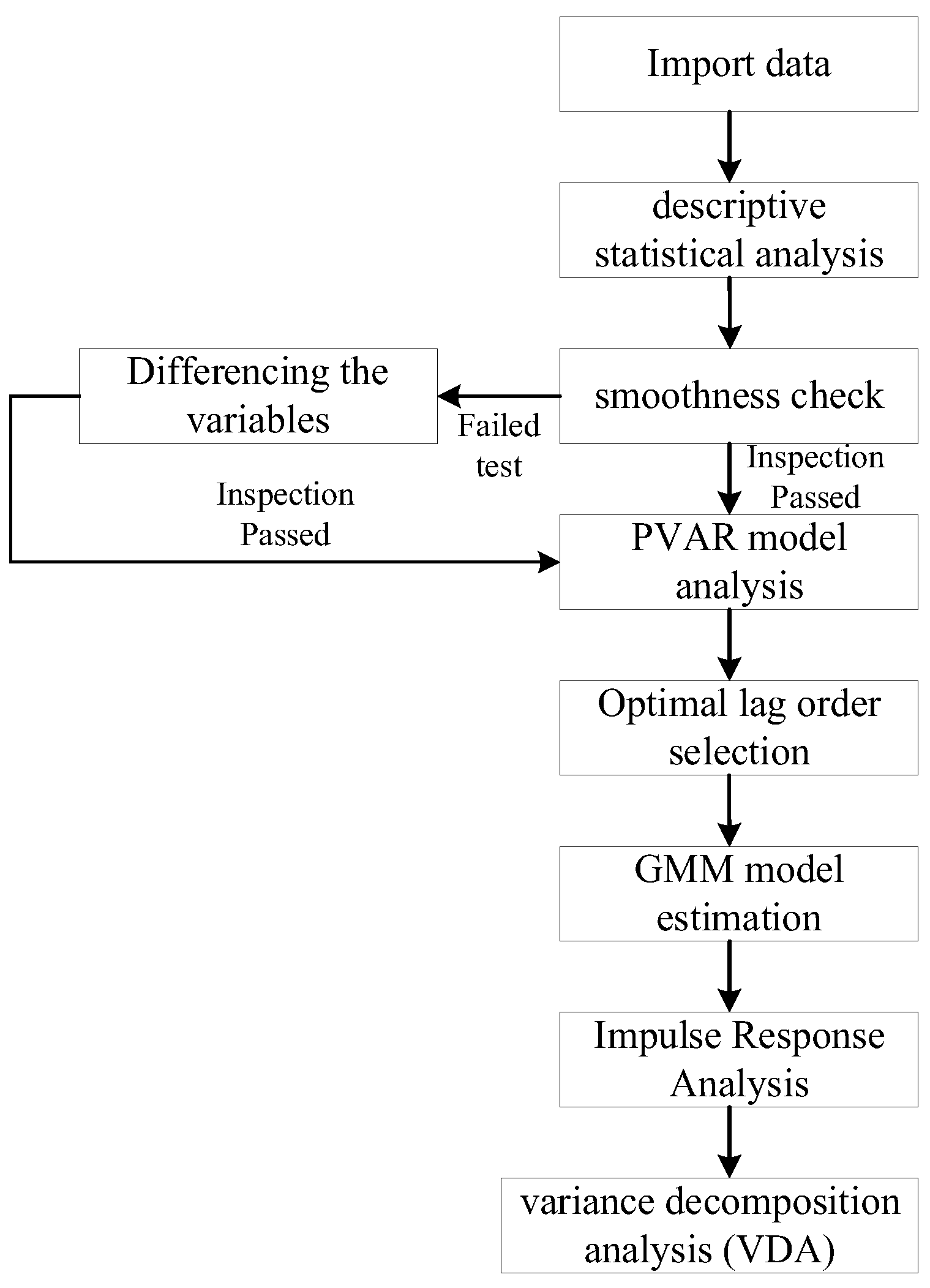
3.3. Optimal Lag-Order Selection

Determining the appropriate lag length for the variables in a Panel Vector Autoregression (PVAR) model is a crucial step. The choice of lag length directly influences the model’s performance and its ability to fit the data accurately. If the lag length is too long or too short, it can reduce the model’s precision by either wasting too many degrees of freedom or failing to capture the model’s dynamic properties adequately.

In this study, the optimal lag order was selected by minimizing the values of criteria that balance model fit with complexity. These criteria include the Modified Akaike Information Criterion (MAIC), Modified Bayesian Information Criterion (MBIC), and Modified Quasi Information Criterion (MQIC). The findings suggest that lag order 1 is the best choice, as indicated by the lowest values of these criteria.

Table 4. Optimal lag-order selection.

Lag	MAIC	MBIC	MQIC
1	−28.0000 *	−181.2611 *	−90.1403 *
2	−26.3265	−128.5011	−67.7539
3	−19.6704	−70.7577	−40.3841

Note: * indicates the optimal lag order chosen in this criterion.

shows that lag order 1 (labeled *) provides the best model fit and complexity control, meaning a one-period lag is optimal for capturing the dynamics of the variables.

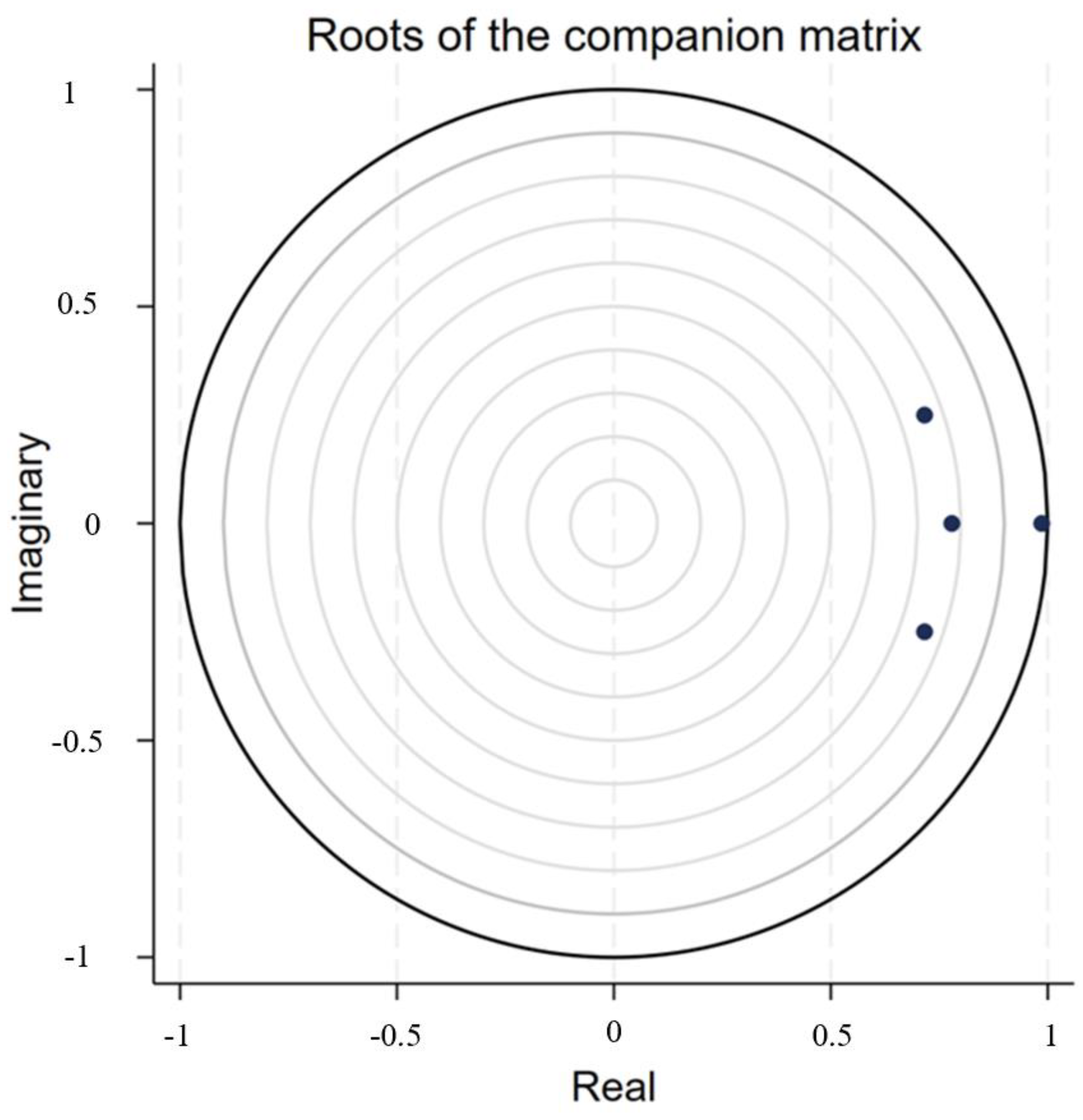
The robustness of the model must be tested to ensure the validity of the estimated model, impulse response, and variance decomposition. This is accomplished by checking if the modulus of the dynamic matrix’s eigenvalue is less than 1 (inside the unit circle). As shown in Figure 2, the PVAR model developed is resilient, confirming its robustness.

3.4. Generalized Moment Estimation (GMM) Model

The PVAR model was estimated and tested using the GMM method. The results of the Panel Vector Autoregression (PVAR) estimation are presented in

Table 5. Results of the PVAR estimation.

Variable	Industrial Subsystem	Economic Subsystem	Energy Subsystem	Carbon Emission Subsystem
L1 (Industry subsystem)	2.9944	−1.6751	−0.1671	0.0080
	(4.0344)	(3.2512)	(0.4171)	(0.1673)
L1 (Economic subsystem)	3.7246	2.0168	−0.2930	−0.0232
	(6.6764)	(5.3836)	(0.6883)	(0.2692)
L1 (Energy subsystem)	1.6246	−1.2643	0.8156	0.0034
	(4.1424)	(3.3484)	(0.3905)	(0.1446)
L1 (Carbon emission subsystem)	−8.5539	6.8232	0.7778	1.3550
	(16.1189)	(13.0103)	(1.6072)	(0.6828)

below. In the table, L1 represents the optimal lag coefficient. The last four columns show the parameter estimation results of the equation, along with the corresponding standard deviations of the parameters.

The projected outcomes show that when the industrial subsystem is used as the explained variable, the coefficients for the economic subsystem, energy subsystem, and carbon emission subsystem with a first-order lag are 3.7246, 1.6246, and −8.5539, respectively. This indicates that both the energy and economic subsystems positively impact the industrial subsystem. However, the influence of energy consumption is less significant than that of economic development, particularly in heavy industries like steel and non-ferrous metals. The industrial subsystem is negatively affected by the carbon emission subsystem. The growth in carbon emissions may lead to higher operating and maintenance costs for heavy industries as they attempt to reduce emissions. Additionally, mergers and restructuring of large-scale heavy industrial businesses create aggregation effects, which make it difficult for some small and medium-sized businesses to survive.

When the economic subsystem is the explained variable, the coefficients for the industrial subsystem, energy subsystem, and carbon emission subsystem are −1.6751, −1.2643, and 6.8232, respectively. This indicates that increasing energy use and expanding heavy industries like steel and non-ferrous metals negatively impact economic growth. The gap in the degree of impact is small, possibly because the development of heavy industries often involves substantial investment. If the investment is overly concentrated and lacks effective regulation, it may lead to redundant construction and inefficient management, causing resource waste and environmental pollution. Additionally, if energy consumption grows too quickly and energy supplies cannot keep up, it may result in energy shortages, which further hinder steady economic expansion. On the other hand, carbon emissions, primarily caused by the burning of fossil fuels, are significant energy sources that drive economic growth. Therefore, adjustments in carbon emissions can have a positive effect on economic development. According to production theory, increasing production factors like energy often leads to higher output and economic growth.

When the energy subsystem is the explained variable, the coefficients for the first-order lagging industrial subsystem, economic subsystem, and carbon emission subsystem are −0.1671, −0.2930, and 0.7778, respectively. This implies that energy use is negatively impacted by heavy industry and economic expansion, particularly in sectors like steel and non-ferrous metals. There may be a shift from dirty to clean energy, with the effects of economic growth becoming more prominent. The influence of economic development itself is positive, meaning economically developed areas tend to promote their own growth. However, energy usage is positively influenced by changes in carbon emissions, suggesting that rising carbon emissions often lead to increased energy consumption, especially from fossil fuels.

When the carbon emission subsystem is the explained variable, the coefficients for the first-order lagging industrial subsystem, economic subsystem, and energy subsystem are 0.0080, 0.0232, and 0.0034, respectively. This indicates that the development of industries like steel and non-ferrous metals, along with the carbon emission system, will benefit from increased energy consumption. Heavy industries, particularly steel, cement, and chemicals, as well as the demand for energy in manufacturing, all contribute to this effect. Fossil fuels such as coal, oil, and natural gas produce large volumes of carbon dioxide and other greenhouse gases when burned for energy. However, the carbon emission system may suffer due to economic progress. As economic development reaches a certain point, the economic structure tends to diversify. This often results in slower energy demand growth, which in turn slows the rate of carbon emissions [38].

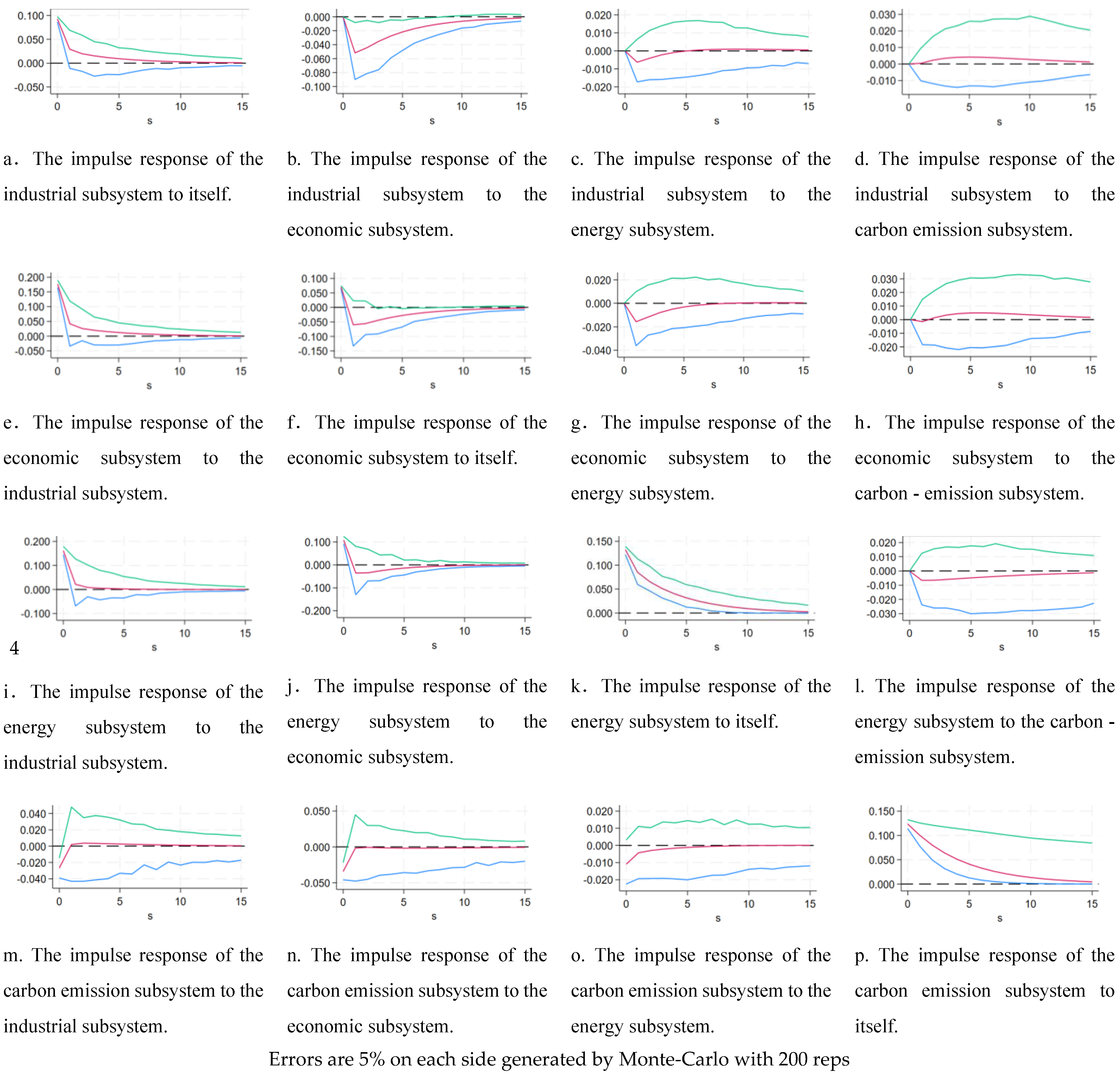
3.5. Pulse Response Function

The GMM model focuses on the short-term perspective and reveals the interactions among the four variables. On the other hand, the PVAR model’s impulse response analysis provides a detailed view of how any variable responds dynamically to disturbances in the other variables. It also shows the precise effects of these disturbances on both present and future values. The plots of the impulse response function offer a clear picture of the interaction between any two variables as well as insight into the long-term patterns of linkage between the variables. To examine how a variable’s response evolves from the short term to the long term when affected by shocks from other variables, we used impulse response analysis in this study. This analysis investigated the impacts of shocks between two of the four selected variables.

In the Figure 3, the horizontal axis depicts the quantity of response periods, which is set to 15 in this paper, while the vertical axis reflects the response status of the variable subjected to the shock. Presented as a red solid line in the graph is the response function. The green and blue lines on both sides indicate positive and negative twice standard deviation deviation bands, respectively. In order to obtain the corresponding impulse response function plots, this paper performed 200 Monte Carlo simulation (Monte Carlo) experiments on the four selected variables.

The analysis results show that the industry subsystem, the energy subsystem and the economic subsystem are very responsive to their own shocks, with significant positive impacts in the first two phases, and their impulse responses all show a convergence trend. In contrast, the carbon subsystem’s response to shocks turns from negative to positive in the first two stages. Overall, all variables stabilize within 15 periods after the shocks, which verifies the robustness of the model and indicates that the impulse response analysis has achieved good results. Next, we conducted more detailed analyses for different variables.

(1) Impact response of the industrial subsystem to other variables.

The response of the economic subsystem to the shock from the industrial subsystem is a negative shock, and the negative shock is more rapid in the first two periods, and then gradually converges until it converges to zero in the 10th period, indicating that when the development of the iron and steel, non-ferrous metals and other industries undergoes a change, the economic development produces a negative response and then this response tends to be stable over time; when the energy subsystem is affected by the shock of the industrial subsystem, the response of the energy subsystem is a negative shock, and the negative response in the first two periods is significant, and then it gradually converges and tends to be stable in the 5th period. When the energy subsystem is impacted by the industry subsystem, the first two periods consist of significant negative impacts, and then gradually converge and level off in the fifth period, indicating that the impacts of industrial development on energy consumption do not trigger a significant response, but only a slight negative impact in the initial period. As time passes, this relationship persists, but its impact gradually weakens and tends to zero. When the carbon emission subsystem is impacted by the industry subsystem, the first five periods show a positive impact; following that, the impact effect gradually diminishes and eventually converges slowly to zero in the tenth period. This suggests that changes in heavy industries like steel, iron, and non-ferrous metals have a relatively flat impact on carbon emissions, with only a slight positive impact before eventually converging to zero.

(2) Impact response of economic subsystems to other variables.

With an impact coming from economic subsystems, the industrial subsystem reacts with a positive impact. In the first two phases, the impact is relatively rapid, then gradually gentle, converging to zero in phase 8 and continuing into period 15. This suggests that when the economic indicators (GDP, etc.) change, this upgrading of the consumption structure further expands the market demand for heavy industrial products such as iron steel, machinery, chemical industry, etc., thus promoting the development of heavy industry. When the energy subsystem is impacted by economic subsystems, the first two periods exhibit a rapidly declining negative shock, then it gradually rises and gradually converges to zero. This suggests that industries with high energy consumption and poor added value will eventually give way to those with low energy consumption and high added value in the industrial structure. This industrial structure’s optimization and modernization can lower the energy usage per output unit, thus reducing energy consumption while achieving economic growth. When the carbon emission subsystem is impacted by economic subsystems, the positive impact and the whole process is relatively flat, showing that with the acceleration of industrialization and urbanization, all kinds of economic activity needs a lot of energy to support it, and out of all of these energy sources, carbon emissions rise as a result of the burning of fossil fuels, which releases a lot of greenhouse gasses like carbon dioxide.

(3) Impact response of the energy subsystem to other variables.

When there is an impact on the sources coming from the energy subsystem, the industrial subsystem in the first two periods shows a relatively rapid positive impact, and after that, it gradually converges to zero, suggesting that an increase in energy consumption is often accompanied by an expanding market demand. When the economy grows and people’s quality of life increases, there is an increasing demand for energy, and this increase in demand has driven the development and growth of related industries. When the economic subsystem is impacted by the energy subsystem, it presents as a rapidly decreasing positive shock before stage 1. Then, it becomes a negative impact, and gradually converges to zero after period 5, showing that energy consumption promotes the birth and development of a number of new industries. The emergence of these new industries not only stimulates economic growth but also fosters the refinement and advancement of the industrial framework. Nevertheless, over-reliance on industries with high energy consumption and emissions, or a limited energy consumption mix, can pose challenges (such as excessive dependence on fossil energy such as coal); such an unreasonable structure will restrict economic development. When the carbon emission subsystem is impacted by the energy subsystem, it shows a rapid negative impact, then gradually converges to zero, showing that the use of fossil fuels is the result of the energy structure progressively shifting from high carbon to low carbon as energy demand increases. The share of energy is steadily diminished, and the adoption of clean energy, which generates minimal carbon emissions, contributes to lowering overall carbon emissions.

(4) Impact response of the carbon emission subsystem on other variables.

Industries with high carbon emissions may face stricter market access restrictions or even be prohibited from doing business in certain regions or countries, which will limit the space for industrial expansion and development. However, in the long run, limiting carbon emissions and setting emission reduction targets can encourage businesses to execute scientific and creative solutions in technology and industrial progress. The industry subsystem shows a negative shock in the first two periods, and the shock is zero in the second period. After that, the shock gradually converges to a positive one. However, eventually, the carbon emission restrictions and the setting of emission reduction targets can stimulate the motivation of businesses to engage in industrial upgrading and technological innovation; when the economic subsystem is subjected to the impact of the carbon emission subsystem, the first two periods show negative impacts, and the impacts become zero after the 2nd period, which indicates that high carbon emissions are often associated with the large consumption of non-renewable resources such as fossil fuels, etc., and that, with the gradual depletion of these resources, economic development will be faced with the constraints of resources, resulting in the rise of the cost of production, which will affect the economic growth potential; when the energy subsystem is impacted by the carbon emission subsystem, it shows a gradually rising negative impact in the first five periods, and converges to zero after the fifth period, indicating that energy usage efficiency has increased dramatically with the ongoing development of clean energy, energy-saving, and emission-reduction technologies. Meanwhile, the use of energy-saving technologies can also successfully lower carbon emissions and energy consumption. These technical developments lower the cost of using renewable energy while simultaneously increasing energy efficiency.

3.6. Analysis of Variance Decomposition

Following the completion of the study of the impulse response function for the dynamic interactions among the four variables, in order to explore the specific impacts of each disturbance term on the endogenous variables in more depth and to precisely depict the interaction effects among the variables, we can adopt the method of variance decomposition. This method can further reveal the long-term interactions among the industrial subsystem, the economic subsystem, the energy subsystem, and the carbon emission subsystem, and analyze in detail the composition of the variance contribution ratio of each variable.

It may be concluded that the variance decomposition findings are comparatively stable since, as

Table 6. Results of the variance decomposition analysis.

Variable Name	S	Industrial Subsystem	Economic Subsystem	Energy Subsystem	Carbon Emission Subsystem
Industrial subsystem	1	1.0000	0.0000	0.0000	0.0000
Economic subsystem	1	0.8630	0.1370	0.0000	0.0000
Energy subsystem	1	0.4720	0.2120	0.3160	0.0000
Carbon emission subsystem	1	0.0410	0.0690	0.0070	0.8830
Industrial subsystem	2	0.7770	0.2200	0.0030	0.0000
Economic subsystem	2	0.7890	0.2050	0.0060	0.0000
Energy subsystem	2	0.4140	0.2020	0.3840	0.0010
Carbon emission subsystem	2	0.0260	0.0440	0.0050	0.9250
Industrial subsystem	3	0.6760	0.3190	0.0040	0.0000
Economic subsystem	3	0.7360	0.2550	0.0080	0.0000
Energy subsystem	3	0.3810	0.2030	0.4150	0.0010
Carbon emission subsystem	3	0.0220	0.0350	0.0040	0.9390
Industrial subsystem	4	0.6280	0.3670	0.0040	0.0010
Economic subsystem	4	0.7070	0.2830	0.0090	0.0000
Energy subsystem	4	0.3640	0.2030	0.4310	0.0020
Carbon emission subsystem	4	0.0200	0.0310	0.0040	0.9450
Industrial subsystem	5	0.6020	0.3920	0.0040	0.0020
Economic subsystem	5	0.6900	0.3000	0.0090	0.0010
Energy subsystem	5	0.3550	0.2020	0.4410	0.0020
Carbon emission subsystem	5	0.0190	0.0300	0.0040	0.9480
Industrial subsystem	6	0.5880	0.4060	0.0040	0.0030
Economic subsystem	6	0.6800	0.3090	0.0090	0.0010
Energy subsystem	6	0.3490	0.2010	0.4470	0.0020
Carbon emission subsystem	6	0.0180	0.0280	0.0040	0.9500
Industrial subsystem	7	0.5790	0.4140	0.0030	0.0040
Economic subsystem	7	0.6740	0.3150	0.0090	0.0020
Energy subsystem	7	0.3640	0.2010	0.4530	0.0020
Carbon emission subsystem	7	0.0180	0.0280	0.0040	0.9510
Industrial subsystem	8	0.5730	0.4190	0.0030	0.0050
Economic subsystem	8	0.6700	0.3180	0.0090	0.0020
Energy subsystem	8	0.3440	0.2000	0.4530	0.0030
Carbon emission subsystem	8	0.0180	0.0270	0.0040	0.9510
Industrial subsystem	9	0.5700	0.4210	0.0030	0.0050
Economic subsystem	9	0.6680	0.3200	0.0090	0.0020
Energy subsystem	9	0.3430	0.2000	0.4550	0.0030
Carbon emission subsystem	9	0.0170	0.0270	0.0040	0.9520
Industrial subsystem	10	0.5680	0.4230	0.0030	0.0060
Economic subsystem	10	0.6660	0.3220	0.0090	0.0030
Energy subsystem	10	0.3420	0.2000	0.4560	0.0030
Carbon emission subsystem	10	0.0170	0.0270	0.0040	0.9520
Industrial subsystem	11	0.5660	0.4240	0.0040	0.0060
Economic subsystem	11	0.6650	0.3220	0.0090	0.0030
Energy subsystem	11	0.3410	0.1990	0.4560	0.0030
Carbon emission subsystem	11	0.0170	0.0270	0.0040	0.9520
Industrial subsystem	12	0.5660	0.4250	0.0040	0.0060
Economic subsystem	12	0.6650	0.3230	0.0090	0.0030
Energy subsystem	12	0.3410	0.1990	0.4570	0.0030
Carbon emission subsystem	12	0.0170	0.0270	0.0040	0.9520
Industrial subsystem	13	0.5650	0.4250	0.0040	0.0070
Economic subsystem	13	0.6640	0.3230	0.0090	0.0030
Energy subsystem	13	0.3410	0.1990	0.4570	0.0030
Carbon emission subsystem	13	0.0170	0.0270	0.0040	0.9520
Industrial subsystem	14	0.5650	0.4250	0.0040	0.0070
Economic subsystem	14	0.6640	0.3230	0.0090	0.0030
Energy subsystem	14	0.3410	0.1990	0.4570	0.0030
Carbon emission subsystem	14	0.0170	0.0270	0.0040	0.9520
Industrial subsystem	15	0.5640	0.4250	0.0040	0.0070
Economic subsystem	15	0.6640	0.3230	0.0090	0.0030
Energy subsystem	15	0.3410	0.1990	0.4570	0.0030
Carbon emission subsystem	15	0.0170	0.0270	0.0040	0.9520

illustrates, the results for periods 10 and 15 are essentially the same. During the fifteenth era, the industrial subsystem is affected by itself and the contribution rate of the economic subsystem, energy subsystem and carbon emission subsystem to its fluctuation is 0.4250, 0.0040, and 0.0070, respectively; that is, in the long run, the industrial structure is more affected by economic development. For the economic subsystem, the contribution rate of the industrial subsystem, energy subsystem and carbon emission subsystem to its fluctuation is 0.6640, 0.0090, and 0.0030, respectively, indicating that the industrial structure mainly affects the change of economic development. For the energy subsystem, except for its own impact, the contribution rate of the industrial subsystem, economic subsystem, and carbon emission subsystem to its fluctuations is 0.3410, 0.1990, and 0.0030, respectively, indicating that energy consumption is more affected by the industrial structure. For the carbon emission subsystem, the contribution rate of the industrial subsystem, economic subsystem, and energy subsystem to its fluctuation is 0.0170, 0.0270, and 0.0040, respectively, indicating that carbon emissions are more affected by themselves.

These findings demonstrate that, in terms of industry, heavy industry with high energy consumption and emissions is gradually giving way to the service industry and emerging businesses that use little energy and produce few emissions as a result of ongoing technological advancements and increased environmental consciousness [40,41,42,43,44]. This shift not only lowers carbon emissions but also increases resource efficiency and fosters high-quality economic development; the economy is moving toward low-carbon, environmentally intensive growth, which has both positive economic and ecological effects. With the continuous development and application of renewable energy technology, the energy consumption structure has gradually shifted from relying on fossil energy to diversified and clean energy, lowering carbon emissions in the process.

4. Conclusions and Recommendations

This study analyzed the dynamic relationships among four subsystems—industry, economy, energy, and carbon emissions—using the PVAR model, based on panel data from 30 Chinese provinces between 2017 and 2021. The results revealed that the industrial and economic subsystems contributed significantly to the growth of carbon emissions, while the energy subsystem helped moderate this increase, especially through the use of clean energy. The study’s findings, supported by impulse response and variance decomposition analyses, demonstrated the gradual shift in the roles of these subsystems over time, with energy’s influence on carbon emissions becoming more pronounced. Compared to the existing literature [45], this study extended the analysis by integrating all four subsystems and capturing the complex, dynamic interactions over time, thus offering a more nuanced understanding of their relationships. Despite the methodological innovations, the study acknowledges limitations, such as the potential for data noise and the exclusion of external factors like policy changes and global economic fluctuations. Future research can build on this work by incorporating more external variables, improving model robustness, and exploring regional variations in the relationships among these subsystems, thereby providing deeper insights for low-carbon transition policies.