Abstract
The accurate identification of drilling conditions is pivotal for optimizing drilling operations. Detailed condition identification enables refined management of the drilling process, facilitates the detection of non-productive time (NPT), and offers actionable insights to improve drilling performance. In this study, a novel predictive model is presented that integrates the Kepler optimization algorithm (KOA) with random forest (RF) for detailed drilling condition identification. This method enhances the granularity of the operation differentiation and improves the classification accuracy. A systematic comparison of various classification algorithms reveals the superior performance of the RF algorithm in accurately identifying drilling conditions. The incorporation of the KOA allows for the refinement of the hyperparameter randomness and for iterative optimization of the RF model’s initial weights and thresholds, leading to optimal classification results. Case studies demonstrate that three predictive models were trained and evaluated. Validation results show that the KOA-RF model achieves an accuracy of 95.65%. To demonstrate the practical applicability of this methodology in enhancing rig efficiency. The KOA-RF algorithm proposed in this study for detailed drilling condition identification can be programmed into software to enable automated, real-time, and intelligent identification of drilling conditions on-site. Key performance indicator (KPI) analysis can be performed based on the identification results, thereby identifying the sources of NPT, optimizing the drilling process, and improving drilling efficiency. In this study, the KOA-RF model achieves detailed drilling condition identification with high accuracy, providing both theoretical contributions and practical value for real-time drilling optimization.
1. Introduction
The integration of artificial intelligence, big data, and related technologies within the petroleum industry offers novel avenues to enhance the efficiency of oilfield operations. Within the realm of field operations, drilling conditions denote specific operational processes. Statistical analysis reveals that the average time efficiency of current drilling construction operations stands at a mere 70%, indicative of substantial time loss [1]. Furthermore, the widespread utilization of recorded data for the real-time monitoring of drilling conditions remains elusive. In traditional practices, physical models and manual empirical diagnosis serve as the primary means for identification, yet these approaches encounter challenges in ensuring both timeliness and accuracy due to the intricacies of highly nonlinear mapping relationships among various feature parameters. Conversely, machine learning techniques offer the capability to capture and model such nonlinear mappings across high-dimensional feature spaces, thereby facilitating effective pattern discrimination tasks. Notably, the literature studies indicate that actual drilling time accounts for only a small portion of the entire drilling project, comprising approximately 70% to 80% of the total duration, with the tripping operation worth 30% of the total drilling time [2]. This includes such conditions as bottom-hole circulation, drilling initiation and cessation, and pre-drilling connections [3]. Consequently, the precise delineation of conventional pull out of hole, trip in hole, and pipe connection conditions enables the generation of meticulous operational reports by the drilling crew, facilitating subsequent time-critical analyses. Such reports furnish rig supervisors and drilling engineers with vital statistics concerning rotary and sliding drilling durations, thereby facilitating efficiency analyses. Moreover, this accumulated data serves as a foundation for the development of algorithms geared towards the detection of aberrant drilling occurrences and subsequent closed-loop control mechanisms.
Drilling time refers to the allocation of time among various operational states during the drilling process, typically represented as percentages of the total operational duration. Analyzing the proportion of time spent in each state is crucial for assessing drilling efficiency and interpreting well history and completion data. Total drilling time consists of productive time—which includes technical limit time, the theoretical minimum required for operations, and invisible lost time, associated with inefficiencies not causing complete stoppage—and non-productive time (NPT), which accounts for delays due to equipment failures, procedural complications, or operational downtime [4]. A schematic illustration of the drilling time structure is provided in Figure 1. Furthermore, the total drilling duration can be divided into specific operational phases, including drilling, pipe connection, tripping out, tripping in, normal condition (e.g., reaming, circulating, wellbore cleaning, etc.), and other auxiliary activities, as depicted in the corresponding Figure 2.
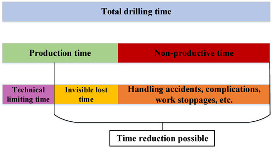
Figure 1.
Division and composition of drilling operation time.
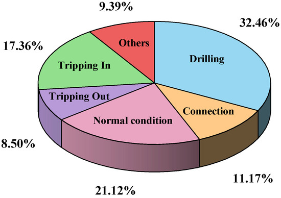
Figure 2.
Total time breakdown chart from test wells.
Utilizing comprehensive logging data to discriminate drilling conditions is a research hotspot and a difficult point for scholars in recent years, and some artificial intelligence and big data technologies have also produced remarkable results.
In 2015, Galina V [5] conducted a comparative analysis of multiple machine learning algorithms for drilling condition identification across 10 conditions. The study identified RF, AdaBoostM2, and RUSBoost as highly reliable classification methods for real-time automated detection of drilling conditions, achieving an accuracy of over 90%. In 2018, Qishuai YIN [6] used mathematical statistics, artificial empirical modeling, and cloud computing to automatically identify eight types of conditions and discover invisible loss time through big data mining technology, thus improving drilling efficiency. The quality control of logging data was carried out through the “3” principle to remove outliers; the relationship between logging parameters and drilling conditions was utilized to carry out real-time drilling conditions identification through computer programming. Furthermore, in 2022, Qishuai YIN [7] proposed a new artificial neural network (ANN) model for rig state classification to recognize eight conditions with 93% accuracy for drilling crew performance evaluation, which resulted in a 45.23% reduction in non-productive time (NPT) and a 31.19% improvement in overall drilling performance. In 2019, Christopher Coley [8] employed 5 machine learning algorithms for drilling condition identification across 15 conditions and tested them on multiple datasets. Based on the F1 score, random forest, decision tree, and k-nearest neighbor classifiers (kNN) demonstrated strong classification performance for previously unseen training data. In contrast, logistic regression and neural network learners performed significantly worse. Additionally, the study found that incorporating engineered features was highly beneficial to the modeling process. In 2019, Sun Ting [9] proposed a support vector machine (SVM) method for drilling condition identification, which analyzes and compares the kernel functions by building multiple intelligent identification models to derive the optimal values of the model parameters. In 2019, Yuxing Ben [10] developed a universal CNN model for drilling condition identification across 16 basins. The CNN model was proven to be the best-performing approach, offering high accuracy, short computation time, and excellent scalability, making it well-suited for big data applications.
In 2021, Francesco Curina [11] compared the accuracy of various machine learning algorithms for drilling condition identification across five conditions and concluded that the optimized random forest model consistently demonstrated high accuracy across all datasets, maintaining an accuracy rate above 90%. However, the study did not specify the optimization methods used. Additionally, the implementation of a system for monitoring rig and equipment parameters was discussed, where machine learning algorithms were applied to optimize drilling, tripping, and casing parameters, thereby reducing NPT. In 2022, Hu [12] developed a data transmission module based on the Wellsite Information Transfer Standard (WITS) and Wellsite Information Transfer Standard Markup Language (WITSML) and created a fusion algorithm model that combines the threshold and neural network methods. In 2022, Mustafa Mohamed Amer [13] employed a support vector machine (SVM) classification model for drilling condition identification across five conditions. The results validated that the model achieved an average accuracy of 85% and a recall rate of 75%, demonstrating its potential to reduce daily morning report data input by 40%. In 2022, Qiao et al. [14] proposed a parallel hybrid model combining a convolutional neural network (CNN) and a bidirectional gated recurrent unit (BiGRU), referred to as CNN-BiGRU, for drilling condition identification. The results demonstrated that this model outperformed individual models, such as CNN, BiGRU, and BiLSTM, achieving an improvement in recognition accuracy of over 6%. Compared to serial hybrid models, the CNN-BiGRU not only improved accuracy by 3% but also doubled the training speed, significantly enhancing computational efficiency. Comparative analysis showed that the proposed method achieved recognition accuracies above 87% for all seven typical drilling conditions, with an overall accuracy reaching 94%. In 2023, Wang Haitao et al. [15] developed a real-time identification model for nine typical drilling conditions by integrating a bidirectional long short-term memory network (BiLSTM) with a conditional random field (CRF). The results indicated that the proposed method significantly improved classification accuracy, achieving a recognition rate of up to 96.49%. In 2023, Yonghai Gao et al. [16] proposed a drilling condition classification method based on an improved stacked ensemble learning approach. By incorporating feature engineering techniques, they enhanced the meta-model components of the stacking algorithm. The model was primarily used to predict eight drilling conditions, achieving both accuracy and recall rates exceeding 90%. In 2024, Ying Qiao [17] combined the encoder layer with an improved graph attention network (GAT) and integrated the K-nearest neighbor (KNN) algorithm to accurately identify seven drilling conditions.
As shown in Table 1, most existing studies on drilling condition identification focus on conventional conditions and lack in-depth recognition of complex or transitional states. The number of identified drilling conditions is generally limited to fewer than 20 categories, which fails to meet the demands of detailed drilling condition identification. This limitation is primarily attributable to the insufficient sensitivity of traditional methods to parameter variations, which hinders the extraction of indicative features from subtle fluctuations in mud logging parameters. As a result, overlapping conditions are difficult to distinguish, and parameter adjustment responsiveness remains insufficient. Moreover, most studies have not emphasized algorithmic structure optimization or multidimensional parameter fusion, thereby constraining model performance in detailed drilling condition identification. Consequently, the high proportion of NPT continues to hinder drilling efficiency improvements.

Table 1.
The differences between this paper and previous works.
To address the current limitations in classification granularity and predictive accuracy in drilling condition recognition, this study employs advanced machine learning algorithms to support detailed drilling condition identification. By classifying 33 distinct conditions—far exceeding the level of differentiation in most existing studies—this work significantly enhances the resolution and interpretability of drilling condition monitoring. A key motivation for this work stems from the observation that traditional methods exhibit low sensitivity to parameter variations, which hinders the extraction of indicative features from subtle fluctuations in mud logging parameters. As a result, overlapping conditions are difficult to distinguish, and parameter adjustment responsiveness remains insufficient. To overcome these challenges, the integration of the Kepler optimization algorithm (KOA) with random forest (RF) introduces a novel optimization framework that improves model performance through adaptive hyperparameter tuning. This approach not only fills a notable gap in the fine-grained classification of complex drilling scenarios but also contributes a high-precision, scalable method for real-time drilling optimization.
2. The Process of Drilling Condition Identification
2.1. Comparison Between Conventional Condition Identification and Detailed Drilling Condition Identification
Drilling conditions refer to the types of conditions in the drilling process that have distinct characteristics and can be differentiated through clear rules. Currently, on-site drilling conditions can be identified through drilling data combined with manual judgment criteria, such as drilling, reaming, back reaming, circulating, trip out, trip in, and connecting. Table 2 presents the basic judgment rules for conventional condition identification [18].
Table 2.
Recognition rules for regular working conditions.
However, conventional condition identification primarily relies on basic drilling parameter indicators. This method often lacks sensitivity to the subtle variations in the drilling process, which may overlook critical information, leading to an increase in invisible lost time and negatively affecting drilling efficiency. For example, conventional condition identification rules cannot effectively differentiate the subtle distinctions between tripping out, tripping in, and connecting. During the drilling string connection phase, conventional condition identification can only distinguish between connected and non-connected states. In contrast, with detailed drilling condition identification, the entire weight-to-weight connection process can be subdivided into the following three parts: weight-to-slip, slip-to-slip, and slip-to-weight. Take the drilling state as an example, where weight-to-slip includes tripping out preparation, short trip out, and setting into slips; slip-to-slip includes connecting; slip-to-weight includes remove slips, short trip in, and connection completed. Similarly, this approach can be extended to other conditions, categorizing the drilling process into drilling (Drlg), tripping out (POH), and tripping in (TIH) states. Each state involves reaming, back reaming, circulating, and connecting. Consequently, the conventional 9 conditions (rotary, sliding, tripping out, tripping in, reaming, back reaming, circulating, connecting and others) are refined into 33 detailed conditions (Table 3).
Table 3.
Results of detailed drilling condition identification.
However, due to the finer segmentation of drilling conditions, relying on traditional rule-based judgment methods may lead to inaccuracies in detailed drilling condition identification, thereby increasing the risk of misjudgment. Such inaccuracies hinder the implementation of fine-grained operational management, making it difficult to monitor subtle transitions between drilling states. As a result, sources of non-productive time (NPT) may go undetected, leading to reduced drilling efficiency and elevated operational costs. To address these challenges, this study leverages machine learning algorithms to achieve detailed drilling condition identification, aiming to enhance recognition accuracy, enable real-time decision-making, and support more efficient and intelligent drilling operations.
2.2. Research Framework of This Study
This study proposes a KOA-RF model for detailed drilling condition identification. This approach leverages data-driven techniques to understand real-time drilling conditions and predict potential issues. The model is designed to learn from real-time data and historical data to improve accuracy and reliability. This paper presents the theoretical foundations and methodological framework for model optimization, detailing the specific optimization process. Finally, the effectiveness of KOA in optimizing the hyperparameters of RF is validated. The results demonstrate that the proposed method can accurately identify multiple drilling conditions, providing an efficient and reliable solution for processing large volumes of logging data.
The workflow for detailed drilling condition identification relies on the following five steps (Figure 3):
- (1)
- Logging data collection from sensor devices;
- (2)
- Data transmission system based on WITSML;
- (3)
- Data preprocessing and construction of the well logging dataset;
- (4)
- Drilling condition identification (manual experience or machine learning—this study focuses on discussing machine learning methods, it be marked * in Figure 3);
- (5)
- Improve drilling performance by real-time monitoring and KPI analysis.
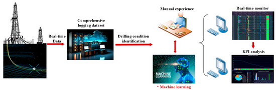
Figure 3.
The process of drilling condition identification.
3. KOA-Optimized RF Model
Random forest (RF) effectiveness largely depends on the selection of hyperparameters, such as the number of decision trees, the maximum number of features considered for splitting at each node, and the maximum depth of the trees. Traditional approaches that rely on random selection or manual tuning are often time-consuming, struggle to find the global optimal solution, and suffer from slow convergence. As a result, the training outcomes can be inconsistent, leading to unstable model performance that fails to achieve optimal results and may even introduce overfitting or underfitting issues. Therefore, to enhance the predictive performance and training efficiency of the RF model, optimization algorithms are introduced to automate hyperparameter selection. The following section presents the optimization algorithm employed in this study.
3.1. RF Algorithm
Random Forest (RF) is a machine learning algorithm composed of an ensemble of in-dependent decision trees, typically based on the Classification and Regression Tree (CART) methodology. It has demonstrated strong performance in classification tasks, making it well-suited for drilling condition identification. Through bootstrap sampling, input training samples are subjected to resampling with replacement to generate diverse training sets. Subsequently, each decision tree produces classification predictions, culminating in the integration of these predictions by the random forest model, as shown in Figure 4. The different colors in the decision trees represent diverse feature splits and classification paths resulting from the use of distinct bootstrap training subsets. The final output is determined through a voting mechanism, with the category receiving the highest number of votes designated as the ultimate result [19].
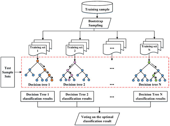
Figure 4.
RF classification algorithm schematic diagram.
3.2. Comparison of Algorithms for Optimizing RF
Since different optimization algorithms vary in their search space for hyperparameters, convergence speed, and ability to achieve the global optimum, a comparative analysis allows for the evaluation of their advantages and disadvantages in terms of accuracy, computational efficiency, and model stability. This study selects three novel optimization algorithms to enhance the random forest model, comparing their optimization strategies to improve the model’s adaptability to complex tasks. The principles of these optimization algorithms are outlined as follows.
3.2.1. Improved Grey Wolf Optimization Algorithm
The IGWO algorithm emulates the hierarchical structure and hunting dynamics observed in gray wolf populations in nature [20]. The specific optimization process is as follows:
Step 1: The Euclidean distance Equation (1) between the current position Xi(t) and the candidate position Xi-gow(t + 1) is used to calculate the radius Ri(t), as follows:
Step 2: The domain Ni(t) of Xi(t) is computed from Equation (2), where Ri(t) is the radius and Di is the Euclidean distance between Xi(t) and Xj(t), as follows:
where Pop represents the current population, i.e., all candidate solutions.
Step 3: Multi-neighborhood learning is performed through Equation (3), where Xn,d(t) is a random neighborhood chosen from Ni(t) and Xr,d(t) is a random wolf chosen from Pop, as follows:
Step 4: Selection and updating is carried out by comparing the fitness values of the two candidate solutions through Equation (4). If the fitness value of the selected candidate is less than Xi(t), Xi(t) is updated by the selected candidate. Otherwise, Xi(t) remains unchanged in the Pop. Equation (4) is as follows:
Step 5: Each iteration counter iter is increased by 1 until the iteration number Maxiter is reached, ending the calculation.
The optimization flowchart is shown in Figure 5, where Xα, Xβ, and Xδ are combinations of hyperparameters in RF, Xα represents the optimal position in the current iteration, i.e., the best hyperparameter combination, which is usually the position with the lowest (or highest) value of the evaluation function. Xβ represents the suboptimal position, which is the combination of hyperparameters with the second lowest value of the evaluation function. Xδ stands for the second-suboptimal position, which is the combination of hyperparameters with the third-lowest value of the evaluation function. D(t) represents the optimal positions of Xα, Xβ, and Xδ.
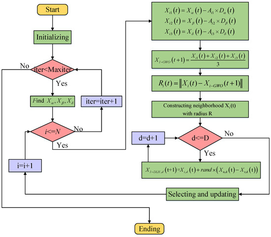
Figure 5.
IGWO flowchart.
3.2.2. Coati Optimization Algorithm
The coati optimization algorithm (COA) mimics two distinct natural behaviors of long-nosed coatis [21], as follows:
Stage I: Hunting and attack strategies for iguanas (exploration phase).
In the exploration phase of the search space, the initial population update of long-nosed raccoons mirrors their strategic behavior observed during iguana attacks. The specific optimization process is as follows:
Step 1: The position of the long-nosed raccoon in the tree is mathematically modeled using the following Equation (5):
Step 2: Once the iguana falls to the ground, it is randomly positioned within the search space. Based on this position, the long-nosed raccoon on the ground traverses the search space and updates its position using the following Equations (6) and (7):
where
N represents the population size.
t represents the current number of iterations.
lbj represents the lower bound of the jth dimensional variable.
ubj represents the upper bound of the jth dimensional variable.
Fitness (t) is used to compute the fitness value.
r denotes a random number between [0, 1].
I denotes a random integer from the set of integers {1,2}.
denotes the new position of the iguana after falling to the ground.
denotes the value of the jth dimension variable for the ith individual under the current iteration.
In short, individuals in the first half of the population climbed trees and updated their positions using Equation (5); individuals in the second half of the population waited on the ground for the iguanas to land and updated their positions using Equations (6) and (7).
Step 3: If the new position computed for each long-nosed raccoon improves the value of the objective function, the new position is acceptable; otherwise, the long-nosed raccoon stays at the previous position. This means performing a greedy selection, as shown in the following Equation (8):
Stage II: Escape from Predators (Development Phase)
To mimic this behavior, random positions are generated near each long-nosed raccoon’s current location, as described in the following Equations (9) and (10):
If the newly calculated position enhances the objective function value, the position is suitable for simulation using Equation (9), which involves performing another greedy selection. The flowchart for the COA algorithm is presented in Figure 6.
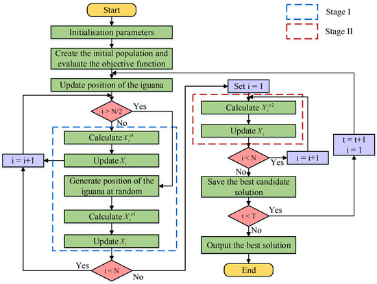
Figure 6.
COA flowchart.
3.2.3. Kepler Optimization Algorithm
The Kepler optimization algorithm, based on Kepler’s laws of planetary motion, is a heuristic optimization method. It mimics the orbital dynamics of planets around the sun to navigate towards optimal solutions, especially when exploring the hyperparameter space to identify the best combinations [22]. The detailed steps are as follows:
Step 1: During initialization, N planets, referred to as the population size, are randomly distributed in d-dimensional space according to the following formula:
where
Xi indicates the ith planet (candidate solution) in the search space.
N represents the number of solution candidates in the search space.
d represents the dimension of the problem to be optimized.
represent the upper bounds.
represent the lower bounds.
rand[0,1] is a randomly generated number between 0 and 1.
Step 2: Calculate gravitational force using Equation (12).
where
and denote the normalized values of and , which represent the masses of and , respectively.
is a small value.
is the universal gravitational constant.
is the eccentricity of a planet’s orbit, which is a value between 0 and 1.
is a value that is randomly generated between 0 and 1;
is the normalized value of that represents the Euclidian distance between and .
Step 3: Calculate the objects’ velocities using the following Equation (13).
where
represents the velocity of object i at time t.
represents object i.
and are randomly generated numerical values at intervals [0, 1].
and are two vectors that include random values between 0 and 1.
and represent solutions that are selected at random from the population.
and represent the masses of and , respectively.
represents the universal gravitational constant.
is a small value for preventing a divide-by-zero error.
represents the distance between the best solution and the object at time t.
represents the semimajor axis of the elliptical orbit of object i at time t.
Step 4: Escaping from the local optimum.
Step 5: Updating the objects’ positions using the following Equation (14):
where
is the new position of object i at time t+1.
is the velocity of object i required to reach the new position.
is the best position of the Sun found thus far.
F is used as a flag to change the search direction.
Step 6: Updates the distance with the Sun using the following Equation (15):
where h is an adaptive factor for controlling the distance between the Sun and the current planet at time t.
Step 7: Implements an elitist strategy to ensure the best positions for planets and the Sun using the following Equation (16):
The specific flowchart is shown in Figure 7.
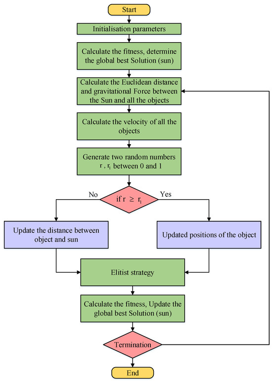
Figure 7.
KOA flowchart.
3.2.4. Comparison of the Optimized RF Results
In this study, the primary optimized hyperparameter combinations are shown in Table 4. Let the optimized hyperparameter combination be defined as follows:
X = (num_trees, max_depth, min_samples_split, min_samples_leaf, max_features).
Table 4.
Parameter description.
Through the above process, the RF algorithm is optimized, and the classification prediction results for the three drilling operational conditions are shown in Figure 8, Figure 9 and Figure 10. In these figures, the input data consist of logging-while-drilling parameters, including variables, such as drilling depth, rate of penetration, hook load, rotary torque, etc. The model outputs the predicted classification results for the drilling conditions. The horizontal axis represents the indices of the test samples, while the vertical axis denotes the corresponding drilling condition classifications. Each test sample’s prediction is plotted against its true label to visualize the model performance. The vertical deviation between the predicted and true values directly reflects the prediction error—smaller deviations indicate better predictive accuracy. It can be clearly observed that the KOA-RF model yields minimal classification error across the test set, thereby achieving the highest prediction accuracy and demonstrating robust generalization capability.
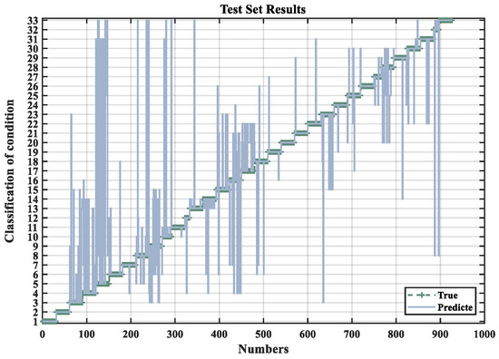
Figure 8.
IGWO-RF prediction results.
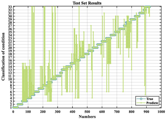
Figure 9.
COA-RF prediction results.
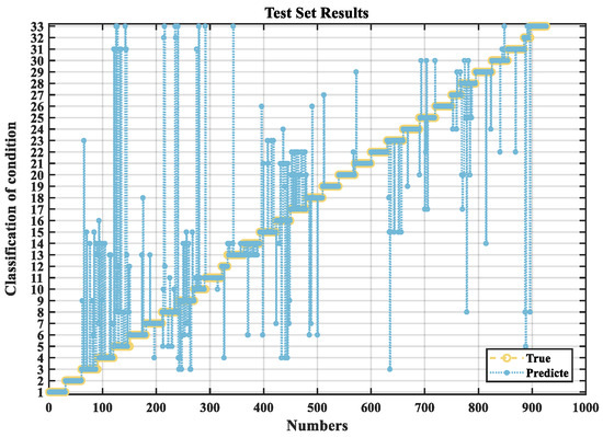
Figure 10.
KOA-RF prediction results.
The experimental findings underscore KOA’s superiority in optimizing the random forest model, particularly evident in the comparison of various parameters, such as accuracy, precision, recall, F1-score, and specificity, among others. These results, presented in the accompanying table, distinctly highlight the superior performance of the KOA-RF model, as shown in Table 5.
Table 5.
Performance comparison of different optimization algorithms for condition prediction.
Based on 10-fold cross-validation, the performance of each model was evaluated with respect to two key metrics, namely accuracy and F1-score, as illustrated in Figure 9. The KOA-RF model consistently achieved accuracy levels ranging from 95.3% to 95.9% across all validation folds, with an average accuracy of 95.65%, which is notably higher than those of the IGWO-RF and COA-RF models. Moreover, the KOA-RF model exhibited a significantly smaller standard deviation, indicating minimal performance fluctuation across different data partitions and demonstrating excellent stability and robustness.
In terms of the F1-score, KOA-RF also showed superior and consistent performance, with scores concentrated in the range of 87.1% to 87.6% and an average F1-score of 87.32%. This highlights its effectiveness in maintaining a balance between precision and recall, making it substantially more competitive than the other models in terms of classification performance.
To further validate the improved performance of the KOA-RF model, an independent sample t-test analysis was conducted based on the results of the 10-fold cross-validation. The results indicate that the KOA-RF model shows significant differences in accuracy compared to the IGWO-RF and COA-RF models, with t-values of 25.68 and 14.52, respectively, and statistical significance with p-values less than 0.001, as shown in Figure 11. The small dots shown on the right side of each box plot represent individual data points of the corresponding classification accuracy results. These dots, overlaid on the kernel density estimation curves, provide a visual distribution of the sample values, helping to illustrate the data spread and concentration around the mean. This enhances the interpretability of the model performance comparison. This suggests that the performance difference between the KOA-RF model and the other two models is highly significant, further confirming the effectiveness and reliability of the KOA-RF model in improving accuracy. Therefore, these findings not only demonstrate the advantage of the KOA-RF model in terms of accuracy but also provide strong statistical support for the improvements made to the model.
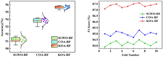
Figure 11.
10-fold cross-validation results of different models.
Upon analyzing the outcomes derived from various optimization algorithms used for random forest parameter optimization, it becomes evident through the examination of multiple graphical representations that the KOA-RF model consistently demonstrates superior performance compared to its counterparts, as shown in Figure 12.
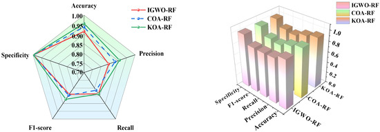
Figure 12.
Comparison results of optimizing random forest models using different algorithms.
As illustrated in the fitness curve comparison in Figure 13, the fitness values of all three optimization algorithms exhibit a decreasing trend with increasing iterations, eventually stabilizing. Among them, KOA-RF demonstrates the fastest convergence rate and attains the lowest final fitness value. In contrast, COA-RF converges more slowly and yields a relatively higher fitness value, while IGWO-RF, despite achieving a slightly lower final fitness value, converges at a comparatively slower rate. These results indicate that the KOA optimization algorithm exhibits the most effective performance in optimizing the hyperparameters of the random forest model.
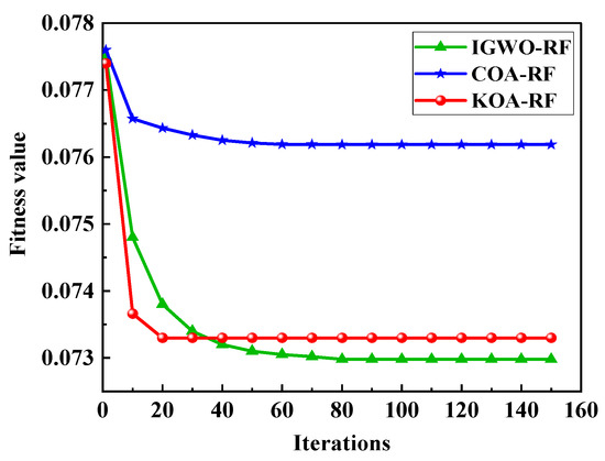
Figure 13.
Comparison of fitness curves.
The receiver operating characteristic (ROC) curves of different models are presented in Figure 14, where the horizontal axis represents the false positive rate (FPR) and the vertical axis denotes the true positive rate (TPR). The ROC curve is a graphical representation used to evaluate the performance of classification models at various threshold settings, illustrating the trade-off between sensitivity and specificity. A curve closer to the upper left corner signifies superior classification performance, as it indicates a higher true positive rate and a lower false positive rate. The analysis reveals that the ROC curves of the optimized models outperform those of traditional algorithms, with KOA-RF’s curve nearly adhering to the upper left corner, demonstrating the best classification performance.
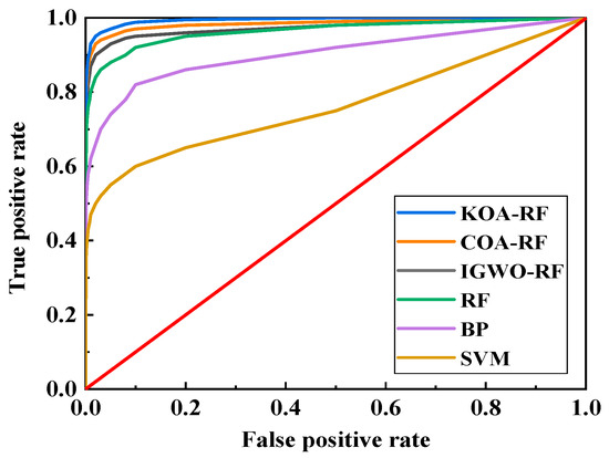
Figure 14.
ROC curve comparison results.
3.3. KOA-RF Model Construction
The performance of a traditional random forest (RF) model is highly dependent on the proper tuning of multiple hyperparameters. Improper parameter settings can result in suboptimal model performance, with training outcomes varying from satisfactory to poor, often necessitating multiple training iterations. The drilling dataset, characterized by a large volume of samples and high feature dimensionality, imposes significant computational demands, while the current algorithm exhibits limited accuracy. To overcome these challenges, the Kepler Optimization Algorithm (KOA) can be employed to optimize the RF model, thereby enhancing its global search capability and training accuracy. The KOA-based RF optimization procedure is illustrated in Figure 15, with its corresponding flowchart presented in Figure 16. The detailed implementation steps are as follows:
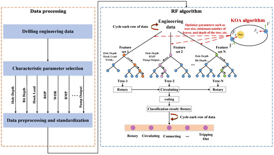
Figure 15.
KOA-RF model schematic diagram.
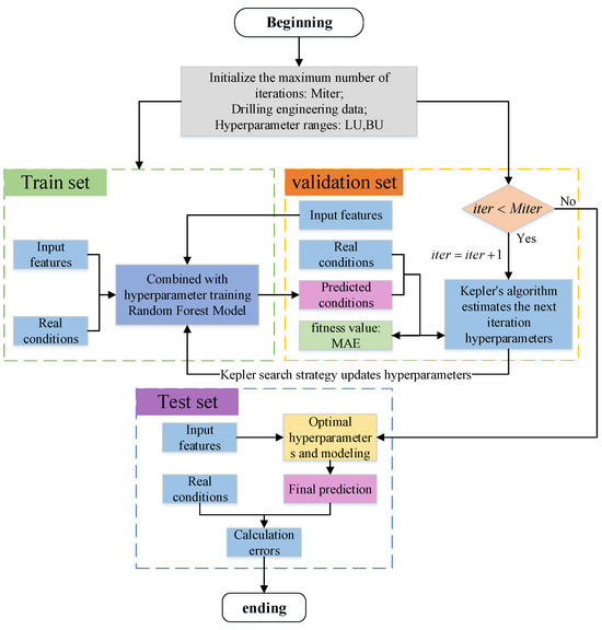
Figure 16.
KOA-RF model flow chart.
Step 1: Initialize random forest parameters;
Step 2: Set the KOA algorithm parameters;
Step 3: Input drilling data for data cleaning, feature selection and normalization;
Step 4: Enter the random forest algorithm, which loops through each row of data in turn for voting;
Step 5: In each iteration, the best combination of hyperparameters of the KOA-optimized random forest is used for training to obtain new predictions;
Step 6: Calculate the error between the prediction result and the true value, which is used to evaluate the effectiveness of the model;
Step 7: Check whether the indicator satisfies the termination condition of the prediction model. If satisfied, output the prediction results; otherwise, continue Step 3 until a satisfactory solution is obtained.
Among them, the blue color on the left represents the input of logging data, which then enters the random forest algorithm. The different colors in the decision trees indicate various feature splits and classification paths arising from distinct bootstrap training subsets. The orange color highlights the prediction results of drilling conditions.
The global search capability of the KOA algorithm is used to optimize the random forest so that the overall model accuracy is improved, the number of training times is reduced, and the computational resources are greatly saved.
4. Application of the KOA-RF Model in Drilling Condition Identification
4.1. Well Example
To demonstrate the application of the proposed KOA-RF model in detailed drilling condition identification, a well from a specific block, namely Well X, was selected for analysis. The well is a horizontal well with a vertical depth of 3230 m and a total drilling depth of 6530 m. The dataset consists of 359 × 194,371 data points, collected over a period of 23 days, which showcases the effectiveness of the proposed algorithm. The well was drilled using five drill bits, with a total drilling time of 175.26 h. The average rate of penetration (ROP) was 12.36 m/h. A subset of the raw data is presented in Figure 17 below.
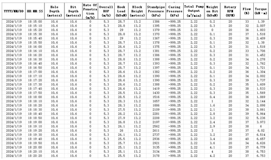
Figure 17.
Partial initial logging data.
4.2. Drilling Data Preprocessing
4.2.1. Feature Selection
The original well logging data encompass multiple key parameters from the drilling process, which thoroughly reflect the diversity and complexity of the drilling conditions. Due to the large number of features, conducting correlation analysis for each parameter individually would be excessively time-consuming and resource-intensive. To optimize the research process and ensure the scientific and rational selection of features, 11 feature parameters were identified based on the drilling process, and these parameters were selected for further study. Their corresponding names are listed in Table 6.
Table 6.
Parameter selection.
4.2.2. Data Preprocessing
Based on the analysis of drilling site data and ensuring the accurate identification of drilling conditions, the frequency required for the model to identify drilling conditions can be simplified to once every 10 s. This moderate sample size clearly represents the trends of each characteristic parameter, making it easier for subsequent machine learning algorithms to extract features and establish long-term dependencies. To effectively support the construction of subsequent machine learning models, data preprocessing is required, which primarily includes the following steps:
- (1)
- Invalid Data Handling
In drilling engineering data processing, invalid data, such as −999.25 and NaN, are typically caused by sensor failures, data transmission errors, or equipment malfunctions. These invalid data points are usually clearly marked in the dataset and can be easily located and deleted using Python 3.11.4’s NumPy and Pandas data processing tools.
- (2)
- Missing Data Handling
Missing data can occur due to sensor failures, incomplete data collection, signal interruptions, and other reasons. Since missing data is rare and much smaller in quantity compared to the overall dataset, it is acceptable to delete the missing data without significantly affecting the overall data quality.
- (3)
- Abnormal Value Handling
Abnormal values are a common issue in data processing. These anomalies may result from equipment malfunctions, sensor errors, or unexpected events, and typically require detection and treatment.
In order to facilitate the subsequent working condition classification prediction, the logging data should be preprocessed, including the processing of missing values, outliers, etc., so as to make the data form a standardized and unified data set. This study utilizes Python tools to clean various parameters. A comparison of the data before and after cleaning is shown in Figure 18.
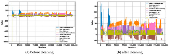
Figure 18.
Comparison of data before and after processing.
4.2.3. Dataset Construction
The cleaned data more accurately reflect the characteristics of the drilling conditions, thereby enhancing the model’s prediction accuracy and its practical value in engineering applications. The cleaned well logging data is shown in Table 7.
Table 7.
Partial drilling parameters data.
4.3. Drilling Condition Identification Based on KOA-RF Model
The KOA algorithm is initialized with a population size of N = 20, and initialize X hyperparameter individuals. The maximum number of iterations is set to Max_iter = 150 and define the search range as [lb, ub] = [0, 200]. Drilling engineering data (well depth, bit depth, WOB, RPM, torque, etc.) are input into the model after undergoing preprocessing and normalization. The random forest (RF) algorithm is employed, with each row of data processed sequentially via majority voting. During this process, indi-viduals are continuously updated based on Kepler’s laws, where each individual ad-justs its position and updates its velocity under gravitational influence. The gravita-tional control mechanism ensures dynamic adjustments around the optimal solution, achieving a balance between global and local searching. The prediction error is calcu-lated between the predicted results and actual values and compute the fitness value to evaluate the model’s effectiveness. We check whether the evaluation metrics meet the termination conditions of the predictive model. If satisfied, the prediction results are generated; otherwise, the iteration process continues until the maximum number of it-erations is reached, obtaining the optimal solution.
The optimized prediction results are shown in the Figure 19 below, with testing conducted on test sets containing 1000 and 3500 samples, respectively. The first 80% of the dataset was used for training, while the remaining 20% was reserved for testing. The average prediction accuracy improved by 5.67% after optimization, demonstrating effective parameter optimization. The detailed optimization results are presented in Table 8 and Table 9.
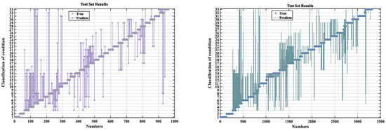
Figure 19.
KOA-RF model test set result graph.
Table 8.
Comparison of performance parameters.
Table 9.
Parameter optimization results.
Overall, the prediction accuracy of KOA-RF for detailed drilling conditions reaches 95.65%, and the confusion matrix of the test set shows that the prediction accuracy of various conditions is high, while the overall effect of the training set is better, as shown in Figure 20. However, the prediction error rate of some conditions is higher than others, e.g., the prediction error rate of the two conditions labeled “Drlg BackReaming” and “Drlg ShortTripOut”, as shown in Figure 17. The error rates are 32.7% and 40%, respectively. This may be caused by the proximity of parameter variations in these two operating conditions. In addition, subsequent studies can continue to supplement the amount of data or increase the differentiation of the characteristic parameters to achieve the best results, with certain complex conditions needing further attention through feature engineering or ensemble modeling.
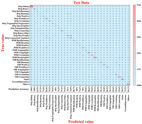
Figure 20.
Confusion matrix for the KOA-RF model test set.
Using the above algorithm and process, detailed drilling condition identification was performed for a specific time interval of the well. Figure 21a shows the identification results for a single day. As can be seen from the figure, the KOA-RF algorithm accurately captures short-term condition changes, identifies high-frequency condition switches, and detects non-productive time. Figure 21b presents the analysis of the identification results over a certain period. The figure shows that the operational conditions for each day are finely classified (with different colored blocks indicating different conditions, for example, the red blocks represent the drilling condition "Drlg Rotary" corresponding to the horizontal axis). These colored blocks can be used to assess the proportion of conditions at various operational stages, identify periodic issues, and optimize overall operational strategies.
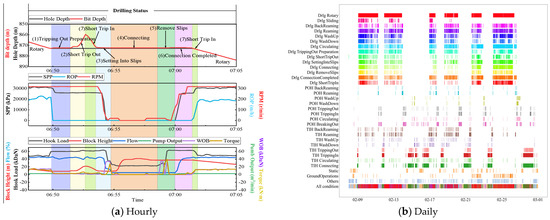
Figure 21.
Detailed drilling condition identification results.
The KOA-RF algorithm proposed in this study for detailed drilling condition identification can be programmed into software (Figure 22 and Figure 23) to enable automated, real-time, and intelligent identification of drilling conditions on-site. Based on the results of detailed condition identification, drilling KPI analysis is conducted to quantify the duration and switching frequency of each condition [23], thereby optimizing drilling operation efficiency.
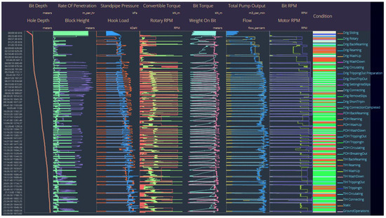
Figure 22.
Real-time monitoring chart (the leftmost side shows the time and feed changes, the middle shows the changes in all kinds of parameters, and the rightmost side shows the results of identifying the drilling conditions at each moment).
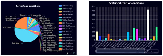
Figure 23.
Drilling KPI analysis chart.
Figure 23 presents the KPI analysis of the drilling conditions. The left panel of Figure 23 allows users to click buttons to display additional legend content, as only part of the legend is currently shown. And it provides a detailed breakdown of the time distribution for each drilling condition and further analyzes the daily and monthly drilling rig operational times. This enables the calculation of the daily proportion of invisible downtime. By conducting an in-depth analysis of the causes behind this downtime, data-driven insights can be provided to optimize the drilling process, ultimately leading to a significant reduction in such time losses.
5. Conclusions
(1) In this study, by leveraging extensive drilling site data, a machine learning-based KOA-RF model was developed to automate the detailed identification of drilling conditions and to perform detailed time analysis for each condition. This approach addresses the limitations of traditional RF models, which are prone to local optimization and are insufficient in analyzing conventional condition times. By enhancing prediction accuracy and identifying sources of invisible time loss, the model provides actionable insights and enables the intelligent classification of detailed drilling conditions along with time analysis.
(2) After comparing the three algorithms of IGWO, COA, and KOA to optimize the RF, the results show that the KOA-RF model is the most effective, with an accuracy rate of 95.65% and an F1-score of 87.23%, which basically meets the field requirements. Based on the identification results of this model, KPI analysis can be conducted to quantify the duration of each drilling condition and identify invisible lost time, thereby optimizing operational efficiency. Furthermore, a software system is proposed to enable automated, real-time, and intelligent identification of on-site drilling conditions. Engineers can take appropriate measures based on the monitoring results to minimize invisible lost time, enhance drilling efficiency, and ultimately reduce drilling costs and time.
(3) In subsequent research, external datasets will be incorporated to conduct further validation, thereby enhancing the generalization capability of the proposed model. Future work will also focus on the intelligent identification of complex working conditions, such as stuck pipes, downhole vibration, and overflow monitoring. By leveraging real-time parameter monitoring to construct machine learning algorithms for early warning of abnormal conditions, the system will assist engineers to make timely adjustments of drilling operations, thus reducing the occurrence of anomalies and improving overall drilling efficiency.
Author Contributions
K.S.: Writing—review and editing, Supervision, Data curation. Z.Z.: Writing—original draft, Validation, Methodology. Z.G.: Validation, Investigation. Y.L.: Resources. J.W.: Validation. M.L.: Validation, Investigation. Z.Y.: Validation, Investigation. J.M.: Resources. All authors have read and agreed to the published version of the manuscript.
Funding
This research was funded by the National Natural Science Foundation of China (Project Number: 51974052), the Chongqing Research Program of Basic Research and Frontier Technology (Project Number: cstc2019jcyj-msxmX0199), and the China National Petroleum Corporation (CNPC) Research Project: “Drilling Safety Control Software” (Project Number: 2024ZZ46-05).
Data Availability Statement
The original contributions presented in the study are included in the article. Further inquiries can be directed to the corresponding author.
Conflicts of Interest
Authors Zhen Guan, Jianhua Wang, Zhiguo Yang and Jintao Mao were employed by the Kunlun Digital Technology Co., Ltd. The remaining authors declare that the research was conducted in the absence of any commercial or financial relationships that could be construed as a potential conflict of interest.
References
- Mohd Mazlan, F.; Ahmad Redzuan, A.Z.; Amiruddin, M.I.; Ramli, A.F.; Slagel, P.; Mondali, M. Optimising Well Times Through Drilling Connection Practices. In Proceedings of the International Petroleum Technology Conference, Online, 23 March–2 April 2021. [Google Scholar] [CrossRef]
- Alsubaih, A.; Albadran, F.; Abbood, N.; Alkanaani, N. Optimization of the Tripping Parameters to Prevent the Surge Related Wellbore Instability. In Proceedings of the ARMA US Rock Mechanics/Geomechanics Symposium, Seattle, WI, USA, 17–20 June 2018. [Google Scholar]
- Cao, D.; Ben, Y.; James, C.; Ruddy, K. Developing an Integrated Real-Time Drilling Ecosystem to Provide a One-Stop Solution for Drilling Monitoring and Optimization. In Proceedings of the SPE Annual Technical Conference and Exhibition, Calgary, AB, Canada, 30 September–2 October 2019. [Google Scholar] [CrossRef]
- Al Hadabi, F.; Al Rashdi, Z.; Al Bulushi, M. Integrated Drilling Services Model Driving Cost Optimization and Operation Efficiency. In Proceedings of the Abu Dhabi International Petroleum Exhibition and Conference, Abu Dhabi, United Arab Emirates, 3–6 November 2023. [Google Scholar]
- Veres, G.; Sabeur, Z. Date Analytics for Drilling Operational States Classifications; Presses Universitaires de Louvain: Louvain-la-Neuve, Belgium, 2015; p. 409. [Google Scholar]
- Yin, Q.; Yang, J.; Zhou, B.; Jiang, M.; Chen, X.; Fu, C.; Yan, L.; Li, L.; Li, Y.; Liu, Z. Improve the Drilling Operations Efficiency by the Big Data Mining of Real-Time Logging. In Proceedings of the SPE/IADC Middle East Drilling Technology Conference and Exhibition, Abu Dhabi, United Arab Emirates, 29–31 January 2018. [Google Scholar] [CrossRef]
- Yin, Q.; Yang, J.; Hou, X.; Tyagi, M.; Zhou, X.; Cao, B.; Sun, T.; Li, L.; Xu, D. Drilling performance improvement in offshore batch wells based on rig state classification using machine learning. J. Pet. Sci. Eng. 2020, 192, 107306. [Google Scholar] [CrossRef]
- Coley, C. Building a Rig State Classifier Using Supervised Machine Learning to Support Invisible Lost Time Analysis. In Proceedings of the SPE/IADC International Drilling Conference and Exhibition, The Hague, The Netherlands, 5–7 March 2019. [Google Scholar] [CrossRef]
- Sun, T.; Zhao, Y.; Yang, J.; Yin, Q.; Wang, W.; Chen, Y. Real-Time Intelligent Identification Method under Drilling Conditions Based on Support Vector Machine. Pet. Drill. Tech. 2019, 47, 28–33. [Google Scholar] [CrossRef]
- Ben, Y.; James, C.; Cao, D. Development and Application of a Real-Time Drilling State Classification Algorithm with Machine Learning. In Proceedings of the 7th Unconventional Resources Technology Conference, Denver, CO, USA, 22–24 July 2019; OnePetro: Richardson, TX, USA, 2019. [Google Scholar] [CrossRef]
- Curina, F.; Abdo, E.; Rouhi, A.; Mitu, V. Rig State Identification and Equipment Optimization Using Machine Learning Models. In Proceedings of the OMC Med Energy Conference and Exhibition, Ravenna, Italy, 28–30 September 2021. [Google Scholar]
- Hu, Z.; Yang, J.; Wang, L.; Hou, X.; Zhang, Z.; Jiang, M. Intelligent identification and time-efficiency analysis of drilling operation conditions. Oil Drill. Prod. Technol. 2022, 44, 241–246. [Google Scholar]
- Amer, M.M.; Otaibi, B.M.; Othman, A.I. Automatic Drilling Operations Coding and Classification Utilizing Text Recognition Machine Learning Algorithms. In Proceedings of the Abu Dhabi International Petroleum Exhibition and Conference, Abu Dhabi, United Arab Emirates, 31 October–3 November 2022. [Google Scholar] [CrossRef]
- Qiao, Y.; Lin, H.; Zhou, W.; Hu, B. Intelligent Identification of Drilling Conditions Based on a Parallel Hybrid CNN-BiGRU Network. In 2022 China Oil and Gas Intelligent Technology Conference—5th High-End Forum on Artificial Intelligence in Petroleum and Petrochemical Industries & 8th Open Forum on Intelligent Digital Oilfields; Beijing Energy Association; China University of Petroleum (Beijing); State Key Laboratory of Oil and Gas Resources and Exploration; State Key Laboratory of Heavy Oil; Baidu AI Cloud. Southwest Petroleum University, School of Computer Science; Sinopec Southwest Oil & Gas Company, Information Management Center: Chengdu, China, 2022; p. 11. [Google Scholar] [CrossRef]
- Wang, H.; Wang, J.; Qiu, C.; Mao, J.; Li, H. Recognition method of drilling conditions based on bi-directional long-short term memory recurrent neural network and conditional random field. Pet. Drill. Prod. Technol. 2023, 45, 540–547+554. [Google Scholar] [CrossRef]
- Gao, Y.; Yu, X.; Su, Y.; Yin, Z.; Wang, X.; Li, S. Intelligent Identification Method for Drilling Conditions Based on Stacking Model Fusion. Energies 2023, 16, 883. [Google Scholar] [CrossRef]
- Qiao, Y.; Luo, Y.; Shang, X.; Zhou, L. An efficient drilling conditions classification method utilizing encoder and improved Graph Attention Networks. Geoenergy Sci. Eng. 2024, 233, 212578. [Google Scholar] [CrossRef]
- Yang, X.; Zhang, Y.; Zhou, D.; Ji, Y.; Song, X.; Li, D.; Zhu, Z.; Wang, Z.; Liu, Z. Drilling conditions classification based on improved stacking ensemble learning. Energies 2023, 16, 5747. [Google Scholar] [CrossRef]
- Breiman, L. Random forests. Mach. Learn. 2001, 45, 5–32. [Google Scholar] [CrossRef]
- Nadimi-Shahraki, M.H.; Taghian, S.; Mirjalili, S. An improved grey wolf optimizer for solving engineering problems. Expert Syst. Appl. 2021, 166, 113917. [Google Scholar] [CrossRef]
- Dehghani, M.; Montazeri, Z.; Trojovská, E.; Trojovský, P. Coati Optimization Algorithm: A new bio-inspired metaheuristic algorithm for solving optimization problems. Knowl.-Based Syst. 2023, 259, 110011. [Google Scholar] [CrossRef]
- Abdel-Basset, M.; Mohamed, R.; Azeem, S.A.A.; Jameel, M.; Abouhawwash, M. Kepler optimization algorithm: A new metaheuristic algorithm inspired by Kepler’s laws of planetary motion. Knowl.-Based Syst. 2023, 268, 110454. [Google Scholar] [CrossRef]
- Saini, G.S.; Hender, D.; James, C.; Sankaran, S.; Sen, V.; van Oort, E. An Automated Physics-Based Workflow for Identification and Classification of Drilling Dysfunctions Drives Drilling Efficiency and Transparency for Completion Design. In Proceedings of the SPE Canada Unconventional Resources Conference, Virtual, 29 September–2 October 2020. [Google Scholar] [CrossRef]
Disclaimer/Publisher’s Note: The statements, opinions and data contained in all publications are solely those of the individual author(s) and contributor(s) and not of MDPI and/or the editor(s). MDPI and/or the editor(s) disclaim responsibility for any injury to people or property resulting from any ideas, methods, instructions or products referred to in the content. |
© 2025 by the authors. Licensee MDPI, Basel, Switzerland. This article is an open access article distributed under the terms and conditions of the Creative Commons Attribution (CC BY) license (https://creativecommons.org/licenses/by/4.0/).