
Probabilistic Modeling and Interpretation of Inaccessible Pore Volume in Polymer Flooding


Abstract
1. Introduction
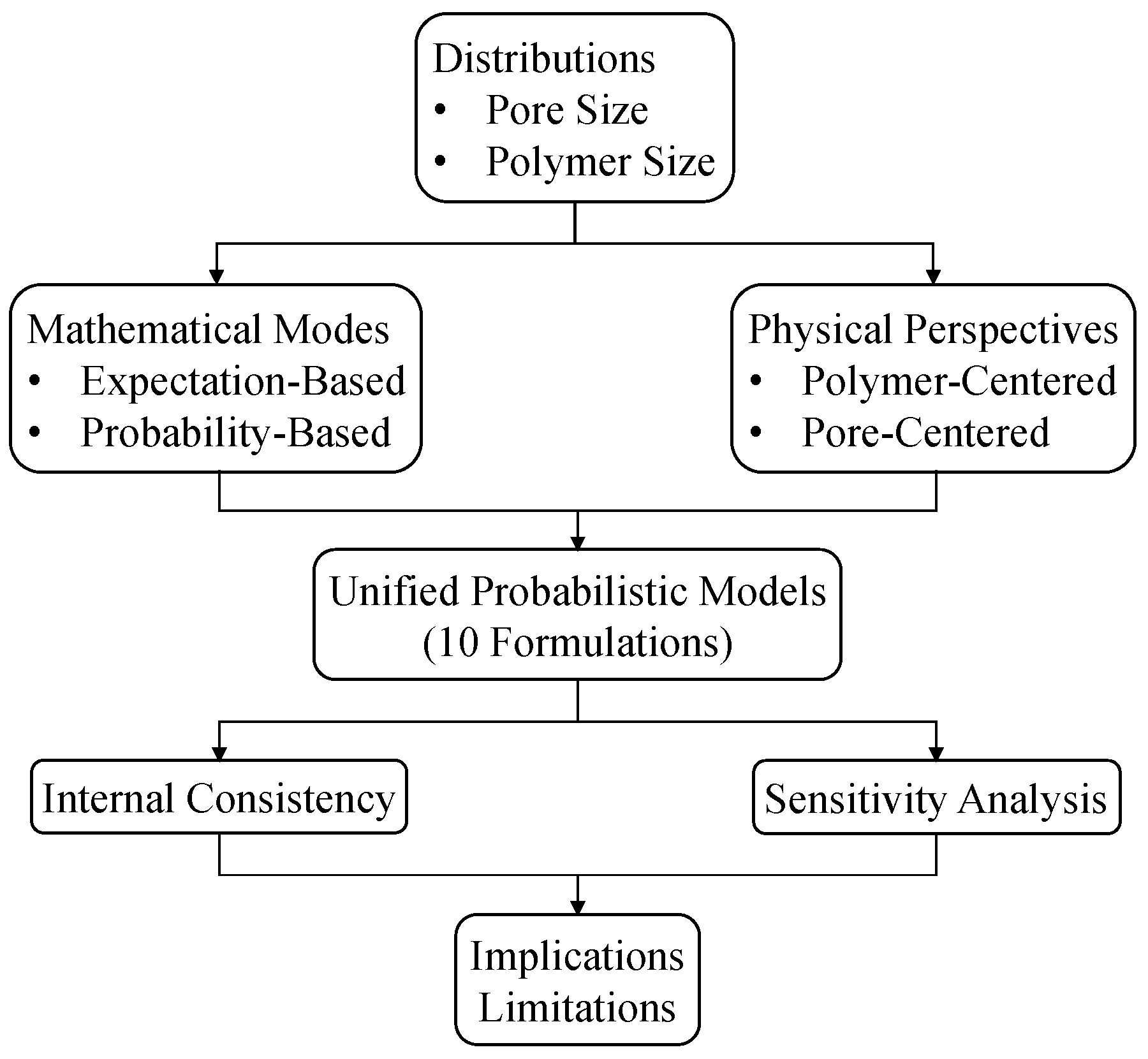
2. Probabilistic Foundation
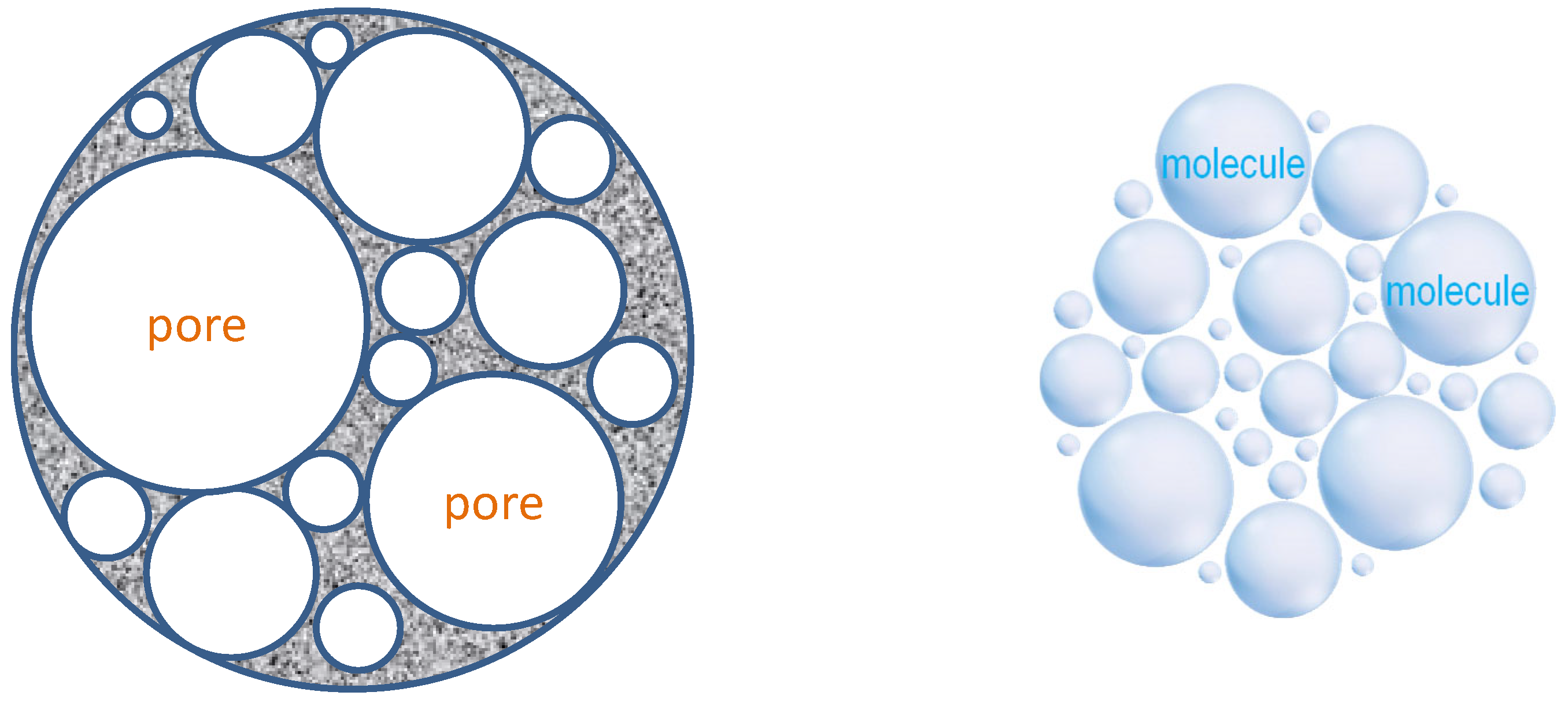
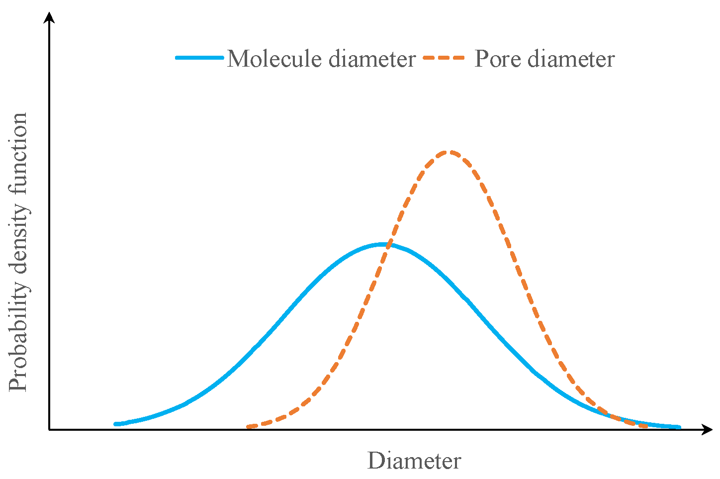
2.1. Randomness in Pore and Polymer Sizes
2.2. Size Exclusion Rule
2.3. Probabilistic Interpretation of the IPVF
2.3.1. Mathematical Standpoint
- Expectation-based interpretation
- Event probability interpretation
2.3.2. Physical Standpoint
- The polymer particle perspective
- The pore perspective
3. Model Formulations
3.1. Modeling Logic and Variable Setup
3.1.1. Assumptions and Variable Definitions
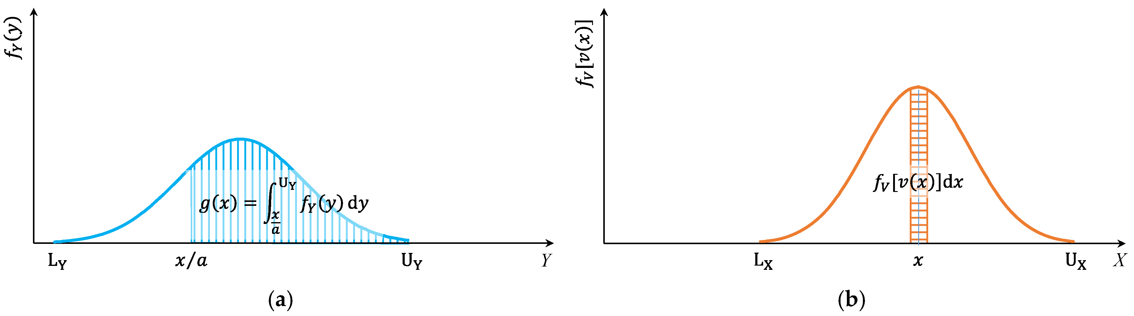
3.1.2. Conversion of Number Probability to Volume Probability
3.2. Expectation-Based Models
3.2.1. From the Perspective of Pores
3.2.2. From the Perspective of Molecules
3.3. Probability-Based Models
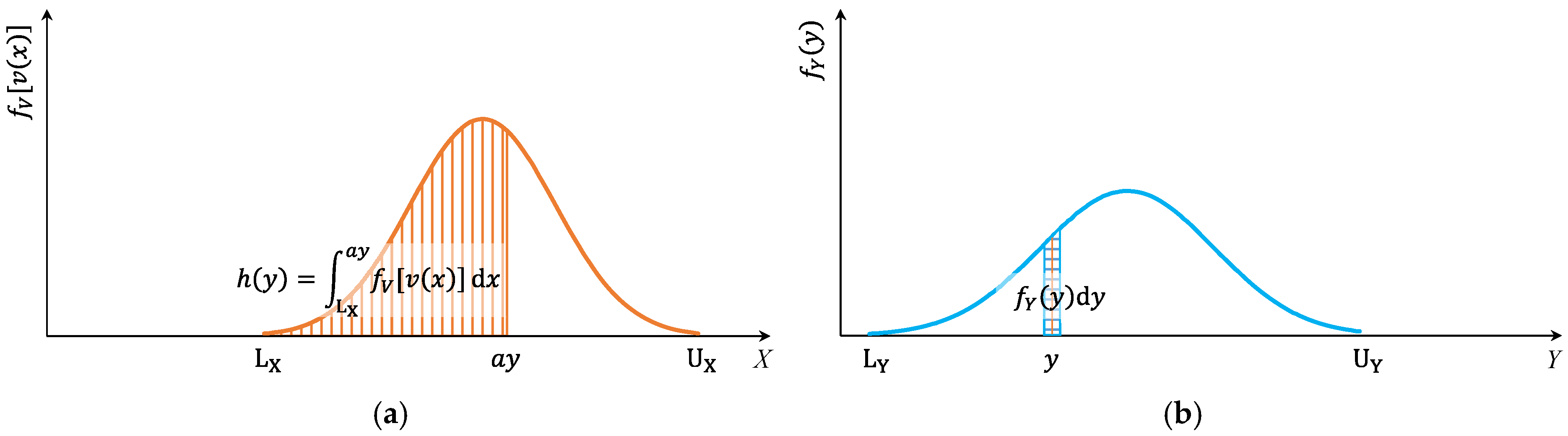
3.3.1. Function Definition
3.3.2. Continuous Cases
3.3.3. Discrete Cases
3.4. Mathematical Equivalence
4. Numerical Evaluation and Model Interpretation
4.1. Synthetic Case Design and Input Configuration
4.2. Model Results, Sensitivity, and Practical Insights
4.2.1. Validation of Model Consistency (Discrete)
4.2.2. Validation of Model Consistency (Continuous)
4.2.3. Sensitivity to Input Distribution and Exclusion Threshold
4.2.4. Physical Interpretation of Simulation Results
4.2.5. Practical Implementation and Model Recommendations
5. Conclusions
6. Future Work
- Validating model predictions using experimental datasets with measured pore and polymer size distributions;
- Investigating the physical basis and calibration of the exclusion factor;
- Extending the framework to hierarchical or network-based pore systems;
- Coupling with additional transport mechanisms such as adsorption or rheological effects;
- Integrating probabilistic IPVF formulations into machine learning workflows for predictive modeling.
Author Contributions
Funding
Data Availability Statement
Conflicts of Interest
Nomenclature
| IPVF | Inaccessible pore volume fraction |
| Pore size (diameter), a stochastic variable | |
| Minimum pore size | |
| Maximum pore size | |
| Molecule size (diameter), a stochastic variable | |
| Minimum molecule size | |
| Maximum molecule size | |
| Size exclusion factor (typically between 3 and 5) | |
| Number probability density function (nPDF) of pores with size corresponding to x | |
| Number probability density function (nPDF) of molecules with size corresponding to y | |
| Number probability mass function (nPMF) of pores with size corresponding to x | |
| Number probability mass function (nPMF) of molecules with size corresponding to y | |
| Volume probability density function (vPDF) of pores with size corresponding to x | |
| Volume probability mass function (vPMF) of pores with size corresponding to x | |
| Mathematical expectation operator | |
| Linear function of X and Y | |
| Probability density function (PDF) of Z | |
| Cumulative distribution function of Z | |
| Probability of event A |
References
- Hassan, A.M.; Zeynalli, M.; Adila, A.S.; Al-Shalabi, E.W.; Kamal, M.S.; Patil, S. Core-to-Field Scale Simulations of Low Salinity Polymer (LSP) Flooding in Carbonate Reservoirs under Harsh Conditions. In Proceedings of the SPE 218223-MS, Tulsa, OK, USA, 22–25 April 2024. [Google Scholar]
- Alexis, D.; Smith, E.; Dwarakanath, V.; Kim, D.H.; Solano, M.; New, P.; Winslow, G. Selection of EOR Polymers for Carbonates from Laboratory Scale to Yard Scale: Observations and Insights. In Proceedings of the SPE 218207-MS, Tulsa, OK, USA, 22–25 April 2024. [Google Scholar]
- Tang, E.; Zhang, J.; Jin, Y.; Li, L.; Xia, A.; Zhu, B.; Sun, X. Optimization of Discontinuous Polymer Flooding Processes for Offshore Oilfields Using a Novel PSO–ICA Algorithm. Energies 2024, 17, 1971. [Google Scholar] [CrossRef]
- Grover, K.; Saadi, J.A.; Farsi, M.A.; Shetty, S.; Villar, J.; Doroudi, A. Utilizing a Design of Experiment Approach in Reservoir Simulation for Pattern Balancing and Optimizing a Polymer Flood. In Proceedings of the SPE 218621-MS, Muscat, Oman, 22–24 April 2024. [Google Scholar]
- Serrano, V.; Ojeda, N.; Tosi, A.; Guillen, P.; Hernandez, L.; Zurletti, A.; Martinez, D.; Campos, H.; Ruiz, A.; Juri, J.E.; et al. Surfactant-Polymer Flooding-Coupling the Development to a Previous Mobile-Modular Polymer Development. In Proceedings of the SPE Improved Oil Recovery Conference, Tulsa, OK, USA, 22–25 April 2024. [Google Scholar]
- Akbari, S.; Mahmood, S.M.; Nasr, N.H.; Al-Hajri, S.; Sabet, M. A Critical Review of Concept and Methods Related to Accessible Pore Volume during Polymer-Enhanced Oil Recovery. J. Pet. Sci. Eng. 2019, 182, 106263. [Google Scholar] [CrossRef]
- AlSofi, A.M.; Wang, J.; AlShuaibi, A.A.; AlGhamdi, F.A.; Kaidar, Z.F. Systematic Development and Laboratory Evaluation of Secondary Polymer Augmentation for a Slightly Viscous Arabian Heavy Reservoir. In Proceedings of the SPE 183793-MS, Manama, Bahrain, 6–9 March 2017. [Google Scholar]
- AlSofi, A.M.; Wang, J.; Kaidar, Z.F. SmartWater Synergy with Chemical EOR: Effects on Polymer Injectivity, Retention and Acceleration. J. Pet. Sci. Eng. 2018, 166, 274–282. [Google Scholar] [CrossRef]
- AlSofi, A.M.; Wang, J.; Leng, Z.; Abbad, M.; Kaidar, Z.F. Assessment of Polymer Interactions with Carbonate Rocks and Implications for EOR Applications. In Proceedings of the SPE 188086-MS, Dammam, Saudi Arabia, 24–27 April 2017. [Google Scholar]
- Najafiazar, B.; Yang, J.; Simon, C.R.; Karimov, F.; Torsæter, O.; Holt, T. Transport Properties of Functionalised Silica Nanoparticles in Porous Media. In Proceedings of the SPE Bergen One Day Seminar, Bergen, Norway, 20 April 2016. [Google Scholar]
- Huh, C.; Bryant, S.L.; Sharma, M.M.; Choi, S.K. pH Sensitive Polymers for Novel Conformance Control and Polymerflood Applications. In Proceedings of the SPE 121686-MS, The Woodlands, TX, USA, 20–22 April 2009. [Google Scholar]
- Dawson, R.; Lantz, R.B. Inaccessible Pore Volume in Polymer Flooding. Soc. Pet. Eng. J. 1972, 12, 448–452. [Google Scholar] [CrossRef]
- Zaitoun, A.; Kohler, N. The Role of Adsorption in Polymer Propagation through Reservoir Rocks. In Proceedings of the SPE 16274-MS, San Antonio, TX, USA, 4–6 February 1987. [Google Scholar]
- Hughes, D.S.; Teeuw, D.; Cottrell, C.W.; Tollas, J.M. Appraisal of the Use of Polymer Injection to Suppress Aquifer Influx and to Improve Volumetric Sweep in a Viscous Oil Reservoir. Soc. Pet. Eng. J. 1990, 5, 33–40. [Google Scholar] [CrossRef]
- Wassmuth, F.R.; Green, K.; Hodgins, L.; Turta, A.T. Polymer Flood Technology for Heavy Oil Recovery. In Proceedings of the PETSOC 2007-182, Calgary, AB, Canada, 12–14 June 2007. [Google Scholar]
- Wan, H.; Seright, R.S. Is Polymer Retention Different under Anaerobic vs. Aerobic Conditions? In Proceedings of the SPE 179538-MS, Tulsa, OK, USA, 11–13 April 2016. [Google Scholar]
- Zhao, J.; Jin, Z.; Hu, Q.; Jin, Z.; Barber, T.J.; Zhang, Y.; Bleuel, M. Integrating SANS and Fluid-Invasion Methods to Characterize Pore Structure of Typical American Shale Oil Reservoirs. Sci. Rep. 2017, 7, 15413. [Google Scholar] [CrossRef]
- Hernando, L.; Alotaibi, M.; Salehi, N.; Zaitoun, A.; Fahmi, M.; Wang, J.; Alfakeer, T.; Mirzayev, K. Designing an In-Depth Conformance Gel System for Carbonate Reservoirs. In Proceedings of the SPE 218181-MS, Tulsa, OK, USA, 22–25 April 2024. [Google Scholar]
- Corredor, L.M.; Espinosa, C.; Delgadillo, C.L.; Llanos, S.; Castro, R.H.; Quintero, H.I.; Cañas, M.C.R.; Bohorquez, A.R.R.; Manrique, E. Flow Behavior through Porous Media and Displacement Performance of a SILICA/PAM Nanohybrid: Experimental and Numerical Simulation Study. ACS Omega 2024, 9, 7923–7936. [Google Scholar] [CrossRef]
- Mezzomo, R.F.; Moczydlower, P.; Sanmartin, A.N.; Araujo, C.H.V. A New Approach to the Determination of Polymer Concentration in Reservoir Rock Adsorption Tests. In Proceedings of the SPE Improved Oil Recovery Conference, Tulsa, OK, USA, 13–17 April 2002. [Google Scholar]
- Manichand, R.N.N.; Seright, R.S.S. Field vs. Laboratory Polymer-Retention Values for a Polymer Flood in the Tambaredjo Field. SPE Reserv. Eval. Eng. 2014, 17, 314–325. [Google Scholar] [CrossRef]
- Mukherjee, S.; Garrido, G.I.; Prasad, D.; Behr, A.; Reimann, S.; Ernst, B. Injectivity, Propagation and Retention of Biopolymer Schizophyllan in Porous Media. In Proceedings of the SPE EOR Conference at Oil and Gas West Asia, Muscat, Oman, 26–28 March 2018. [Google Scholar]
- Poellitzer, S.; Florian, T.; Clemens, T. Revitalising a Medium Viscous Oil Field by Polymer Injection, Pirawarth Field, Austria. In Proceedings of the SPE Europec featured at EAGE Conference and Exhibition, Amsterdam, The Netherlands, 8–11 June 2009. [Google Scholar]
- Lötsch, T.; Müller, T.; Pusch, G. The Effect of Inaccessible Pore Volume on Polymer Coreflood Experiments. In Proceedings of the SPE International Conference on Oilfield Chemistry, Phoenix, Arizona, 9–11 April 1985. [Google Scholar]
- Lund, T.; Bjørnestad, E.Ø.; Stavland, A.; Gjøvikli, N.B.; Fletcher, A.J.P.; Flew, S.G.; Lamb, S.P. Polymer Retention and Inaccessible Pore Volume in North Sea Reservoir Material. J. Pet. Sci. Eng. 1992, 7, 25–32. [Google Scholar] [CrossRef]
- Alfazazi, U.; Thomas, N.C.; Al-Shalabi, E.W.; AlAmeri, W. Investigation of the Effect of Residual Oil and Wettability on Sulfonated Polymer Retention in Carbonate under High-Salinity Conditions. SPE J. 2024, 29, 1091–1109. [Google Scholar] [CrossRef]
- Ferreira, V.H.S.; Moreno, R.B.Z.L. Modeling and simulation of laboratory-scale polymer flooding. Int. J. Eng. Technol. 2016, 16, 24–33. [Google Scholar]
- Osterloh, W.T.; Law, E.J. Polymer Transport and Rheological Properties for Polymer Flooding in the North Sea. In Proceedings of the SPE Improved Oil Recovery Conference, Tulsa, OK, USA, 19–22 April 1998. [Google Scholar]
- Al-Hashmi, A.R.; Divers, T.; Al-Maamari, R.S.; Favero, C.; Thomas, A. Improving Polymer Flooding Efficiency in Oman Oil Fields. In Proceedings of the SPE 179834-MS, Muscat, Oman, 21–23 March 2016. [Google Scholar]
- Al-Maamari, R.S.; Al-Hashami, A.R.; Al-Sharji, H.H.; Dupuis, G.; Bouillot, J.; Templier, A.; Zaitoun, A. Development of Thermo-Gels for in Depth Conformance Control. In Proceedings of the SPE Asia Pacific Enhanced Oil Recovery Conference, Kuala Lumpur, Malaysia, 11–13 August 2015. [Google Scholar]
- Divers, T.; Al-Hashmi, A.R.; Al-Maamari, R.S.; Favero, C. Development of Thermo-Responsive Polymers for CEOR in Extreme Conditions: Applicability to Oman Oil Fields. In Proceedings of the SPE EOR Conference at Oil and Gas West Asia, Muscat, Oman, 26–28 March 2018. [Google Scholar]
- Dupuis, G.; Antignard, S.; Giovannetti, B.; Gaillard, N.; Jouenne, S.; Bourdarot, G.; Morel, D.; Zaitoun, A. A New Thermally Stable Synthetic Polymer for Harsh Conditions of Middle East Reservoirs. Part I. Thermal Stability and Injection in Carbonate Cores. In Proceedings of the Abu Dhabi International Petroleum Exhibition and Conference, Abu Dhabi, United Arab Emirates, 13–16 November 2017. [Google Scholar]
- Gaillard, N.; Giovannetti, B.; Favero, C.; Caritey, J.-P.; Dupuis, G.; Zaitoun, A. New Water Soluble Anionic NVP Acrylamide Terpolymers for Use in Harsh EOR Conditions. In Proceedings of the SPE Improved Oil Recovery Symposium, Tulsa, OK, USA, 12–16 April 2014. [Google Scholar]
- Pancharoen, M.; Thiele, M.R.; Kovscek, A.R. Inaccessible Pore Volume of Associative Polymer Floods. In Proceedings of the SPE 129910-MS, Tulsa, OK, USA, 24–28 April 2010. [Google Scholar]
- Manrique, F.R.; Rousseau, D.; Bekri, S.; Djabourov, M.; Bejarano, C.A. Polymer Flooding for Extra-Heavy Oil: New Insights on the Key Polymer Transport Properties in Porous Media. In Proceedings of the SPE 172850-MS, Mangaf, Kuwait, 8–10 December 2014. [Google Scholar]
- Li, K.; Jing, X.; He, S.; Wei, B. Static Adsorption and Retention of Viscoelastic Surfactant in Porous Media: EOR Implication. Energy Fuels 2016, 30, 9089–9096. [Google Scholar] [CrossRef]
- Idahosa, P.E.G.; Oluyemi, G.F.; Oyeneyin, M.B.; Prabhu, R. Rate-Dependent Polymer Adsorption in Porous Media. J. Pet. Sci. Eng. 2016, 143, 65–71. [Google Scholar] [CrossRef]
- AlSofi, A.M.; Liu, J.S.; Han, M. Numerical Simulation of Surfactant–Polymer Coreflooding Experiments for Carbonates. J. Pet. Sci. Eng. 2013, 111, 184–196. [Google Scholar] [CrossRef]
- Hatzignatiou, D.G.; Norris, U.L.; Stavland, A. Core-Scale Simulation of Polymer Flow through Porous Media. J. Pet. Sci. Eng. 2013, 108, 137–150. [Google Scholar] [CrossRef]
- Leng, J. Simulation Study of Macromolecules Inaccessible Pore Volume Mechanism in Heterogeneous Porous Media. Int. J. Sci. Res. 2021, 10, 396–403. [Google Scholar] [CrossRef]
- Lüftenegger, M.; Clemens, T. Chromatography Effects in Alkali Surfactant Polymer Flooding. In Proceedings of the SPE 185793-MS, Paris, France, 12–15 June 2017. [Google Scholar]
- Stavland, A.; Jonsbraten, H.; Lohne, A.; Moen, A.; Giske, N.H. Polymer Flooding Flow Properties in Porous Media versus Rheological Parameters. In Proceedings of the SPE 131103-MS, Barcelona, Spain, 14–17 June 2010. [Google Scholar]
- Li, J.; Liu, Y.; Guo, S.; Li, B. A Method for Calculating Inaccessible Pore Volume of Polymer. Petrol. Geol. Oilfield Dev. Daqing 2008, 27, 114–117. [Google Scholar]
- Zhang, W.; Sun, L.; Qi, M.; Ye, Y. Laboratory Experiment on Inaccessible Pore Volume of Polymer Flooding. J. Petrochem. Univ. 2016, 29, 35. [Google Scholar] [CrossRef]
- Li, Z.; Dean, R.M.; Lashgari, H.; Luo, H.; Driver, J.W.; Winoto, W.; Pope, G.A.; Thach, S.; Dwarakanath, V.; Mathis, L.; et al. Recent Advances in Modeling Polymer Flooding. In Proceedings of the SPE Improved Oil Recovery Conference, Tulsa, OK, USA, 22–25 April 2024. [Google Scholar]
- El Hana, A.; Hader, A.; Hajji, Y.; Amallah, L.; Hariti, Y.; Tarras, I.; Boughaleb, Y. Stochastic Process Describing Fluid Flow in Porous Media: Langevin Dynamics. Mater. Today Proc. 2022, 66, 396–401. [Google Scholar] [CrossRef]
- Fleurant, C.; van der Lee, J. A Stochastic Model of Transport in Three-Dimensional Porous Media. Math. Geol. 2001, 33, 449–474. [Google Scholar] [CrossRef]
- Tartakovsky, A.M.; Tartakovsky, D.M.; Meakin, P. Stochastic Langevin Model for Flow and Transport in Porous Media. Phys. Rev. Lett. 2008, 101, 44502. [Google Scholar] [CrossRef] [PubMed]
- Delgoshaie, A.H. Stochastic Models for Flow and Transport in Heterogeneous Porous Media; Stanford University: Stanford, CA, USA, 2018. [Google Scholar]
- Serebe, Y.A.A.; Ouedraogo, M.; Sere, A.D.; Sanou, I.; Zagre, W.-K.J.E.; Aubert, J.-E.; Gomina, M.; Millogo, Y. Optimization of Kenaf Fiber Content for the Improvement of the Thermophysical and Mechanical Properties of Adobes. Constr. Build. Mater. 2024, 431, 136469. [Google Scholar] [CrossRef]
- Juang, C.H.; Lovell, C.W. Measurement of Pore-Size Density Function in Sand. Trans. Res. Record 1986, 1089, 97–101. [Google Scholar] [CrossRef]
- Sakurovs, R.; He, L.; Melnichenko, Y.B.; Radlinski, A.P.; Blach, T.; Lemmel, H.; Mildner, D.F.R. Pore Size Distribution and Accessible Pore Size Distribution in Bituminous Coals. Int. J. Coal Geol. 2012, 100, 51–64. [Google Scholar] [CrossRef]
- Brandrup, J.; Immergut, E.H. Polymer Handbook, 3rd ed.; Wiley-Interscience: New York, NY, USA, 1989. [Google Scholar]
- Fetters, L.J.; Hadjichristidis, N.; Lindner, J.S.; Mays, J.W. Molecular Weight Dependence of Hydrodynamic and Thermodynamic Properties for Well-Defined Linear Polymers in Solution. J. Phys. Chem. Ref. Data 1994, 23, 619–640. [Google Scholar] [CrossRef]
- Flory, P.J. Principles Of Polymer Chemistry; Cornell University Press: New York, NY, USA, 1953. [Google Scholar]
- Calhoun, A. Multilayer Flexible Packaging, 2nd ed.; William Andrew: Oxford, UK, 2016. [Google Scholar]
- Abrams, A. Mud Design to Minimize Rock Impairment Due to Particle Invasion. J. Pet. Technol. 1977, 29, 586–592. [Google Scholar] [CrossRef]
- Cozic, C.; Rousseau, D.; Tabary, R. Novel Insights into Microgel Systems for Water Control. SPE Prod. Oper. 2009, 24, 590–601. [Google Scholar] [CrossRef]
- Wang, D.; Cheng, J.; Wu, J.; Wang, G. Experiences Learned after Production of More than 300 Million Barrels of Oil by Polymer Flooding in Daqing Oil Field. In Proceedings of the SPE 77693-MS, San Antonio, TX, USA, 29 September–2 October 2002. [Google Scholar]
- Yan, D.D.; Li, Y.Q.; Dong, D.F.; Wang, F.Y.; Gu, J.X. Study on Matching Relationship of Polymer Hydrodynamic Size and Pore Throat Size for Stratum in Sand Reservoir. In Proceedings of the OTC 24682-MS, Kuala Lumpur, Malaysia, 25–28 March 2014. [Google Scholar]
- Sheng, J.J.; Leonhardt, B.; Azri, N. Status of Polymer-Flooding Technology. J. Can. Pet. Technol. 2015, 54, 116–126. [Google Scholar] [CrossRef]
- Li, Z.; Yang, H.; Sun, Z.; Espinoza, D.N.; Balhoff, M.T. A Probability-Based Pore Network Model of Particle Jamming in Porous Media. Transp. Porous Media 2021, 139, 419–445. [Google Scholar] [CrossRef]


| Types | Advantages | Disadvantages | References | |
|---|---|---|---|---|
| Tracer-based core flooding | Single-slug method | Simple implementation with a single polymer flood cycle | Potential inaccuracies with unfavorable mobility ratios | [7,8,9,10,11,12] |
| Double-slug method | Highly reliable due to repeated flood cycles | Time-intensive due to multiple injection steps | [13,14,15,16,17,18,19,20,21,22,23,24,25,26,27,28,29,30,31,32,33,34] | |
| Tracer-free core flooding | Half concentration method | Streamlined process without tracer necessity | Accuracy compromised in fractured media or large dead volumes | [35,36,37] |
| Numerical simulation | Avoids laboratory-based determination | Computationally demanding, requires extensive data calibration | [38,39,40,41] | |
| Empirical model | Minimal experimental data needed (one polymer flood cycle and RRF data) | Lack of independent verification | [39,42] | |
| Deterministic exclusion method | Straightforward analytical method | Oversimplification by using a singular polymer size value | [43,44] | |
| Cutoff model | Convenient and user-friendly | Arbitrary nature affecting reliability | [45] | |
| Formulation Logic | Expectation-BASED | Probability-Based | ||
|---|---|---|---|---|
| Input Types | Continuous | Discrete | Continuous | Discrete |
| Equations | Equations (10) and (14) | Equations (12) and (16) | Equations (20a)–(20d) | Equations (23a) and (23b) |
| Pairs | Equation (10) ≡ Equation (20a) | |||
| Equation (14) ≡ Equation (20b) | ||||
| Equation (12) ≡ Equation (23a) | ||||
| Equation (16) ≡ Equation (23b) | ||||
| Cases | Types of Variables | μm | μm | ||
|---|---|---|---|---|---|
| #1 |
| = 2.0 = 12.0 | Interval = 0.10 | = 1.0 = 2.0 | Interval = 0.05 |
| #2 | Interval = 0.10 | ||||
| #3 | Interval = 0.20 | Interval = 0.05 | |||
| #4 | Interval = 0.10 | ||||
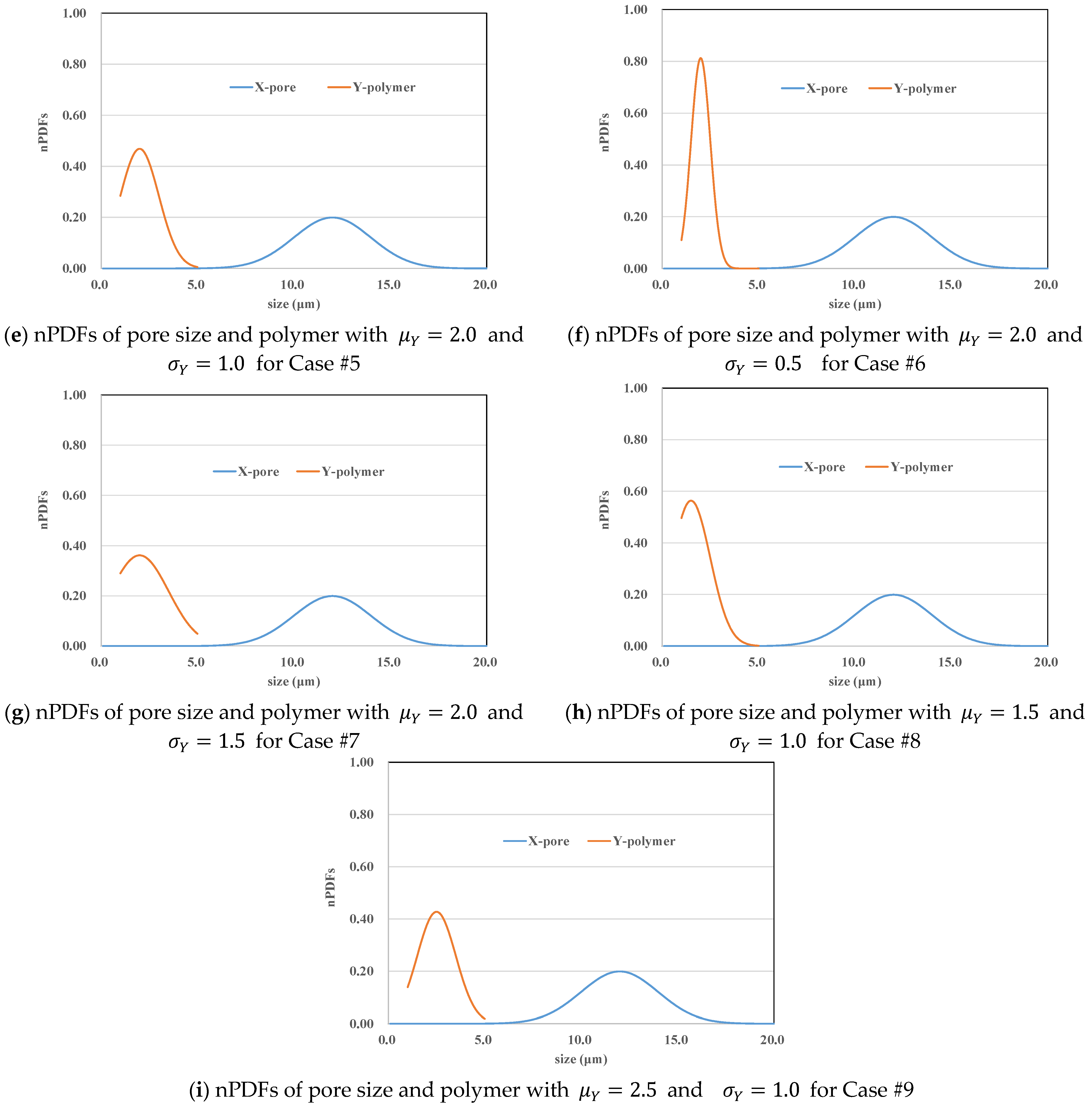
| #5 |
| = 2.0 = 12.0 | ; | ||
| #6 | ; | ||||
| #7 | ; | ||||
| #8 | ; | ||||
| #9 | ; | ||||
| Cases | Sampling Intervals | a = 3.0 | a = 5.0 | |||
|---|---|---|---|---|---|---|
| X | Y | Equations (12)/(23a) | Equations (16)/(23b) | Equations (12)/(23a) | Equations (16)/(23b) | |
| #1 | 0.10 | 0.05 | 0.0367 | 0.0367 | 0.3713 | 0.3713 |
| #2 | 0.10 | 0.10 | 0.0392 | 0.0392 | 0.3832 | 0.3832 |
| #3 | 0.20 | 0.05 | 0.0356 | 0.0356 | 0.3676 | 0.3676 |
| #4 | 0.20 | 0.10 | 0.0380 | 0.0380 | 0.3794 | 0.3794 |
| Cases | a = 3.0 | a = 5.0 | ||||||||
|---|---|---|---|---|---|---|---|---|---|---|
| Equations (10)/(20a) | Equations (14)/(20b) | Equation (20c) | Equation (20d) | Equations (10)/(20a) | Equations (14)/(20b) | Equation (20c) | Equation (20d) | |||
| #5 | 1.0 | 2.0 | 0.0359 | 0.0358 * | 0.0359 | 0.0359 | 0.3685 | 0.3685 | 0.3685 | 0.3685 |
| #6 | 0.5 | 2.0 | 0.0034 | 0.0034 | 0.0034 | 0.0034 | 0.2065 | 0.2065 | 0.2065 | 0.2065 |
| #7 | 1.5 | 2.0 | 0.0907 | 0.0894 * | 0.0907 | 0.0907 | 0.4740 | 0.4740 | 0.4740 | 0.4740 |
| Cases | a = 3.0 | a = 5.0 | ||||||||
|---|---|---|---|---|---|---|---|---|---|---|
| Equations (10)/(20a) | Equations (14)/(20b) | Equation (20c) | Equation (20d) | Equations (10)/(20a) | Equations (14)/(20b) | Equation (20c) | Equation (20d) | |||
| #5 | 1.0 | 2.0 | 0.0359 | 0.0358 * | 0.0359 | 0.0359 | 0.3685 | 0.3685 | 0.3685 | 0.3685 |
| #8 | 1.0 | 1.5 | 0.0160 | 0.0160 | 0.0160 | 0.0160 | 0.2437 | 0.2437 | 0.2437 | 0.2437 |
| #9 | 1.0 | 2.5 | 0.0746 | 0.0742 * | 0.0746 | 0.0746 | 0.5209 | 0.5209 | 0.5209 | 0.5209 |
Disclaimer/Publisher’s Note: The statements, opinions and data contained in all publications are solely those of the individual author(s) and contributor(s) and not of MDPI and/or the editor(s). MDPI and/or the editor(s) disclaim responsibility for any injury to people or property resulting from any ideas, methods, instructions or products referred to in the content. |
© 2025 by the authors. Licensee MDPI, Basel, Switzerland. This article is an open access article distributed under the terms and conditions of the Creative Commons Attribution (CC BY) license (https://creativecommons.org/licenses/by/4.0/).
Share and Cite
Zhao, C.; Zhao, Y.; Zhan, S. Probabilistic Modeling and Interpretation of Inaccessible Pore Volume in Polymer Flooding. Processes 2025, 13, 1720. https://doi.org/10.3390/pr13061720
Zhao C, Zhao Y, Zhan S. Probabilistic Modeling and Interpretation of Inaccessible Pore Volume in Polymer Flooding. Processes. 2025; 13(6):1720. https://doi.org/10.3390/pr13061720
Chicago/Turabian StyleZhao, Chuanfeng, Yifan Zhao, and Shengyun Zhan. 2025. "Probabilistic Modeling and Interpretation of Inaccessible Pore Volume in Polymer Flooding" Processes 13, no. 6: 1720. https://doi.org/10.3390/pr13061720
APA StyleZhao, C., Zhao, Y., & Zhan, S. (2025). Probabilistic Modeling and Interpretation of Inaccessible Pore Volume in Polymer Flooding. Processes, 13(6), 1720. https://doi.org/10.3390/pr13061720