Three-Dimensional Geomechanical Modeling and Hydraulic Fracturing Parameter Optimization for Deep Coalbed Methane Reservoirs: A Case Study of the Daniudi Gas Field, Ordos Basin

Abstract

Deep coalbed methane (CBM) resources represent a significant opportunity for future exploration and development. The combination of horizontal well drilling and hydraulic fracturing technology has emerged as the most efficient method for extracting deep CBM. By optimizing the fracturing parameters for horizontal wells, we can improve the effectiveness of reservoir stimulation even further. In this paper, taking the deep coalbed methane in the Daniudi gas field in the Ordos Basin as the research object, using Numerical simulation software such as Petrel, comprehensively considering the field logging, logging data and laboratory experimental data of rock mechanical parameters, the three-dimensional geomechanical and stress field model of deep coalbed methane is established, and on this basis, the numerical simulation research on the fracture network expansion and construction parameter optimization of single well and well group is carried out. Through the qualitative evaluation of fracture network morphology, the change of in situ stress field, the quantitative evaluation of post-pressure conductivity and fracture volume, the section spacing, construction fluid volume, and construction displacement under the conditions of single well and well group were optimized. The results show that under the condition of a certain well spacing, the fracture propagation of the well group is affected by stress shadowing and channeling, and the fracture pattern is more complex, and the construction scale is smaller than that of a single well. These findings provide critical insights for improving the efficiency of deep CBM recovery.

1. Introduction

With advancements in exploration technologies, deep subsurface energy resources have garnered increasing attention [1,2]. As a critical component of unconventional energy, China’s deep CBM exploration has achieved significant breakthroughs [3]. Estimates suggest that CBM resources at depths exceeding 2000 m exceed 40.7 × 10¹² m³ [4,5]. Deep CBM reservoirs are characterized by high in situ stress, formation pressure, and temperature (“triple-high” conditions) [6]. Challenges such as low permeability, structural complexity, and substantial heterogeneity hinder effective stimulation and produce low well productivity [7]. Horizontal wells with hydraulic fracturing aim to create complex fracture networks, yet optimizing fracture propagation in deep CBM reservoirs remains understudied.

CBM, a self-sourced and self-reserved unconventional natural gas adsorbed in coal seams, exhibits significant differences in genetic and development mechanisms compared to conventional oil and gas reservoirs [8]. This results in distinct variations in attribute modeling between CBM geological and conventional reservoir modeling [9]. Scholars have recently attempted to characterize coal reservoirs using geological modeling techniques quantitatively. Huai et al. achieved differentiation between coal seams and non-coal attributes through facies-controlled 3D modeling [10]. Ma et al. established permeability models by correlating coal permeability with stress and coal lithology [11]. Chen et al. constructed 3D coal structure models using single-well coal structure characterization [12]. Liu investigated pressure drop characteristics during CBM drainage using geological modeling [13]. Li et al. quantitatively analyzed the impact of coal structure on productivity based on coal structure models [14]. Lü developed multi-layer 3D models through characterization of coal seam roof and floor surfaces [15]. Zhou et al. established gas content models using relationships between logging parameters (depth, density, natural gamma, and resistivity) and gas content [16].

Numerous studies have been conducted on numerical simulation and parameter optimization of hydraulic fracture propagation in deep CBM reservoirs. Ren et al. utilized CT scanning and triaxial hydraulic fracturing experiments to investigate hydraulic fracture initiation and propagation in bedded deep coal seams, revealing that bedding planes with lower fracture energy significantly influence fracture behaviour [4]. Wang et al. conducted supercritical CO₂ fracturing experiments demonstrating its effectiveness in enhancing fracture complexity [17]. A Qi et al. proposed a volume fracturing technology for Shenfu deep CBM reservoirs in Ordos Basin, featuring “multi-cluster limited-entry perforation, composite fluid fracturing (high-viscosity fluid for rock breaking + low-viscosity fluid for complex fractures), and multi-size proppant combinations” [18]. Li et al. optimized horizontal well length and completion parameters through numerical simulation based on 79 production wells in Shenfu Block [19]. Yang et al. developed large-scale extreme-volume fracturing technology addressing challenges in deep coal seams, such as high plasticity and difficult proppant placement [20]. Liu Xiao conducted field tests comparing fracture networks under different treatment scales, establishing optimal stimulation practices [21]. Xiong et al. demonstrated enhanced stimulation effects through multi-stage diversion processes based on microseismic monitoring [22]. Tian et al. established a 2D fluid–solid coupling finite element model using ABAQUS to simulate fracture propagation [23]. Zhao et al. revealed weak structural surfaces’ significant impacts on fracture patterns through actual triaxial experiments and acoustic emission monitoring [24].

To a certain extent, these studies have clarified the hydraulic fracture propagation law of coalbed methane, optimized the hydraulic fracturing parameters of deep coalbed methane, and proposed the corresponding hydraulic fracturing technology, but these studies have not carried out the geological modeling research of deep coalbed methane reservoirs, nor have they designed the optimization of hydraulic fracture parameters of well groups under the influence of stress shadow during deep coalbed methane fracturing. In this paper, the three-dimensional geological model of deep coalbed methane in the Ordos Basin-Yuyang favorable block is first established, and then the numerical simulation of construction parameters optimization under the conditions of hydraulic fracturing of a single well and a well group of deep coalbed methane is carried out. The results of this paper show that hydraulic fracturing of deep coalbed methane has certain guiding significance.

2. Geological Setting Area

The primary productive coal seams are located in deep coal reservoirs beneath 2000 m. Structurally, the field typically features a gentle monocline that slopes from the northeast (higher elevation) to the southwest (lower elevation), with an average gradient of 6–9 m per kilometer. The formation dip angles range from 0.3° to 0.6°. Additionally, there are locally developed, nose-shaped uplifts that exhibit orientations striking nearly east to west.

According to the comprehensive logging interpretation diagram of a pilot hole in the target block, the depth of the Tai 1 section is 2851.50–2874.00 m, the apparent thickness is 22.50 m, and the lithology is black coal, gray coal, gray-black mudstone, and limestone. The location of the target horizon 8# coal is 2851.50–2865.00 m, the apparent thickness is 14.50 m, and the mudstone is sandwiched with 2.5 m in the middle. The gas saturation result is 8.3~26.3%, and the average gas saturation is 22% (

Table 1. Logging interpretation result table.

Layer Number	Measuring Depth (m)	Visual Thickness (m)	Vertical Depth (m)	Porosity (%)	Permeability (mD)	Gas Saturation (%)	Interpret Conclusions
1	2798.5–2801.7	3.2	2738.75–2741.85	5.6	0.29	26.4	Gas-bearing layer
2	2806.8–2811.9	5.1	2746.79–2751.74	7.7	0.57	33.8	Differential gas layer
3	2830.2–2834.2	4	2769.47–2773.34	4.8	0.19	28.3	Gas-bearing layer
4	2836.8–2838.5	1.7	2775.85–2777.50	7	0.42	28.9	Gas-bearing layer
5	2850.7–2855.1	4.4	2789.31–2793.57	7.7	0.54	46.3	Differential gas layer
6	2862.0–2865.4	3.4	2800.25–2803.54	5.2	0.02	12.4	Carbonaceous mudstone
7	2869.3–2870.7	1.4	2807.31–2808.67	6.7	0.35	22.3	Coal
8	2880.1–2882.0	1.9	2817.77–2819.61	7.2	0.32	27.8	Coal
9	2884.8–2897.1	12.3	2822.33–2834.25	4.6	0.19	22.1	Dry layer
10	2897.9–2904.6	6.7	2835.02–2841.52	5.9	0.42	31.3	Coal
11	2904.6–2909.4	4.8	2841.52–2846.17	2.8	0.71	17.4	Dry layer
12	2909.4–2911.5	2.1	2846.17–2848.21	4.5	0.04	11.2	Carbonaceous mudstone

). The structure of 8# coal body is relatively complete, which is the primary-fractured type, and the macroscopic type of coal and rock is mainly the semi-bright type, followed by the bright type, a small amount of the semi-dark type and dull type, and is interbedded with multiple layers of carbonaceous mudstone and gray or black mudstone with a thickness of 2–3 m. The degree of thermal evolution of coal is moderate, and the Ro of coal rock is between 1.2~1.7%, which belongs to medium metamorphic degree, medium and low volatile bituminous coal; the cleavage and fractures formed by thermal metamorphism and tectonic action are relatively developed.

To enhance production capacity, horizontal wells combined with large-scale volume fracturing are employed onsite to create complex fracture networks. However, optimizing key parameters for such large-scale volume fracturing operations requires further investigation. This study will conduct 3D geomechanical modeling of deep coalbed methane reservoirs and perform fracturing parameter optimization research based on field-derived parameters.

3. Three-Dimensional Geological and Mechanical Modeling

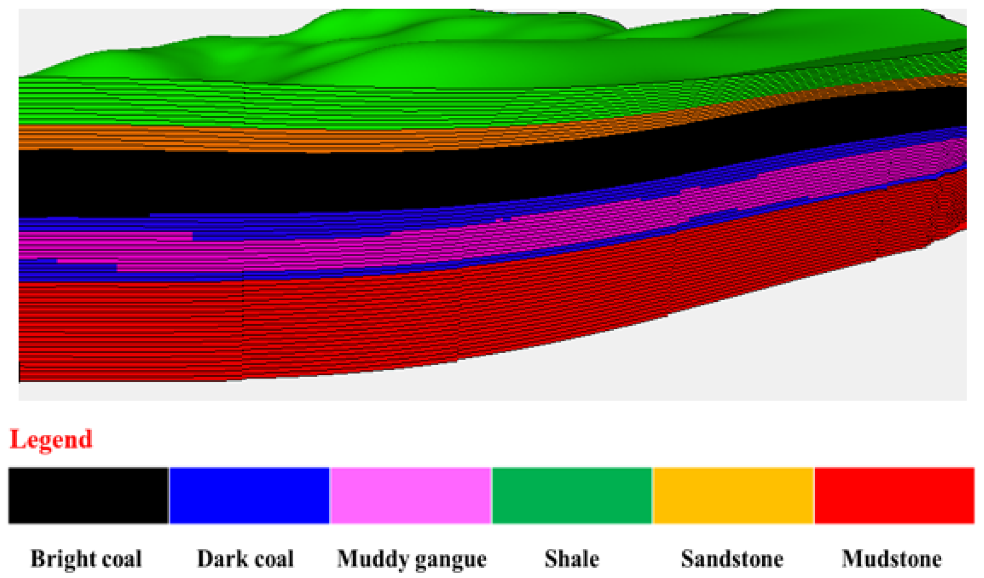
3.1. Geological Facies Modeling

Data were imported from 282 wells, including information on wellhead, deviation, stratification, logging, and wellbore trajectory, into Petrel. After defining the boundaries based on the logging interpretation results of the target block, the pay zones were identified as four layers: T2-3-T2-2-T2-1-T1-2-T1-1. The target area covers approximately 38 square kilometers, with a pay zone thickness of about 14 m. The grid step size was set to 25 m × 25 m in the horizontal plane and 1 m in the vertical direction. Figure 1 is a schematic diagram of the construction model.

The petrofacies division standard, shown in

Table 2. Standard table of lithofacies division.

Lithofacies	Truncated Value
Bright coal	GR ≤ 60GAPI, DEN ≤ 1.6 g/cm3, LLD > 3000 Ω.cm
Semi-bright coal	60 < GR < 100GAPI, DEN ≤ 1.6 g/cm3, LLD > 3000 Ω.cm
Semi-dark coal	100 ≤ GR < 120GAPI, 1.6 < DEN ≤ 1.85 g/cm3, LLD > 500 Ω.cm
Dull coal	120 ≤ GR < 140GAPI, 1.6 < DEN ≤ 1.85 g/cm3, LLD > 500 Ω.cm
Gangue	GR < 140GAPI, DEN ≤ 2 g/cm3
Limestone	GR < 60GAPI, DEN > 2 g/cm3, CNL ≤ 7%
Semi-dark coal	100 ≤ GR < 120GAPI, 1.6 < DEN ≤ 1.85 g/cm3, LLD > 500 Ω.cm
Dull coal	120 ≤ GR < 140GAPI, 1.6 < DEN ≤ 1.85 g/cm3, LLD > 500 Ω.cm

, was formulated by comparing the logging curves such as gamma, density, and deep lateral resistance with the logging data while drilling. The pay zones primarily consist of bright coal along with carbonaceous mudstone and shale, which are overlain by sandstone and limestone and underlain by mudstone.

Figure 2 is the reservoir lithofacies profile. The roof is about 10 m thick and is a limestone–sandstone formation. The coal seam is about 14 m thick, with bright coal on top and 2–3 m of carbonaceous mudstone partings in the middle and lower part. The lower part is mainly semi-bright and semi-dark coal. The floor is about 8 m thick and mainly mudstone.

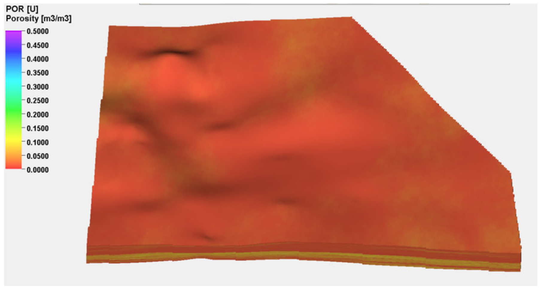
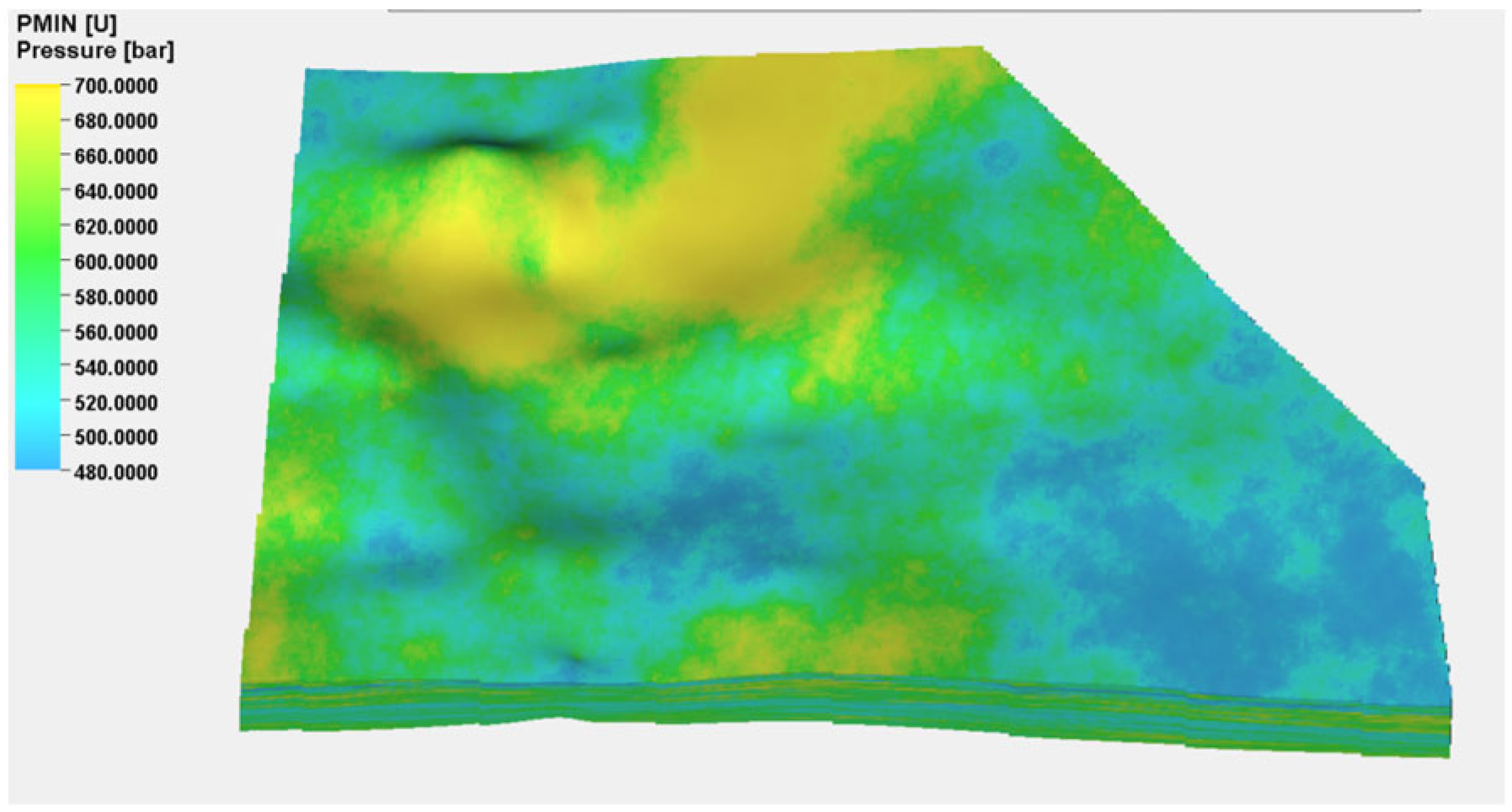
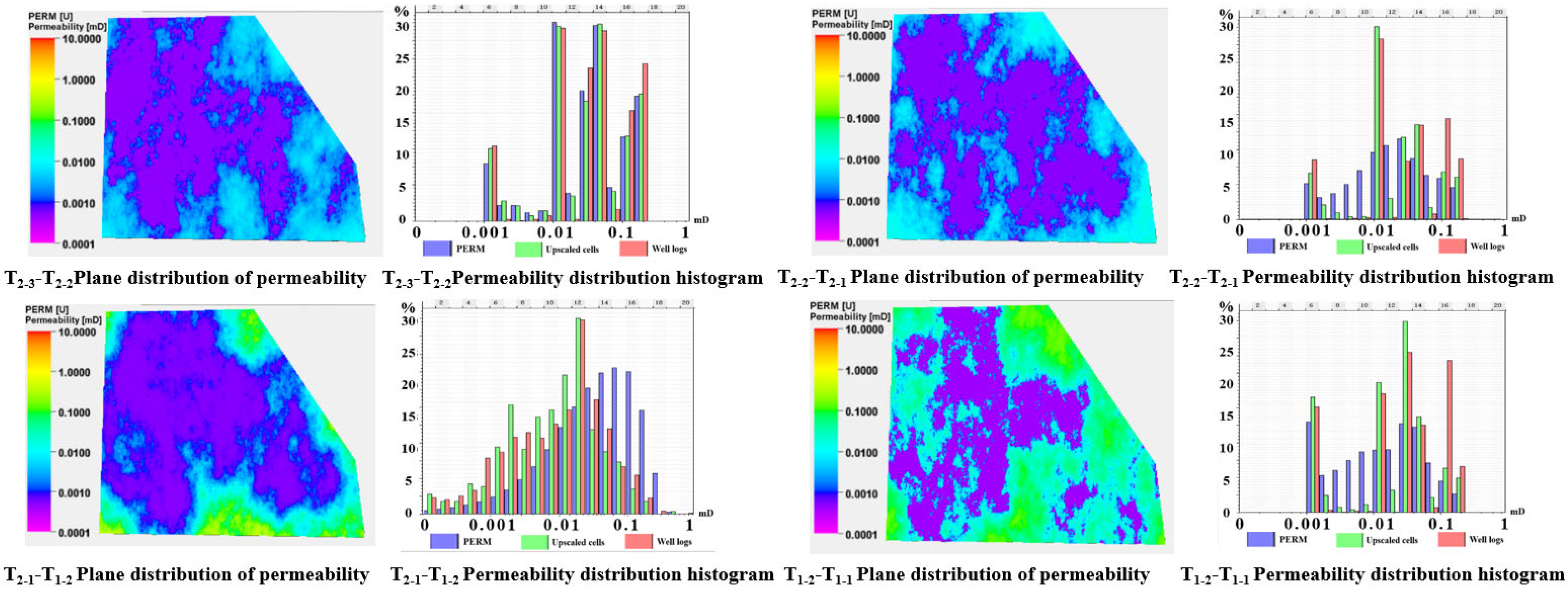
3.2. Geological Property Modeling

Due to the strong correlation between coal seam density and porosity and permeability, the empirical formula for calculating coal seam porosity and permeability using density logging data can be obtained through regression, and the porosity and permeability logging interpretation curves in the target block are calculated by using the density logging curve. The porosity and permeability profiles of each single well are obtained after comparison and correction with the logging data.

Porosity:

$$POR=38.725e^{-1.291\ast DEN}$$

(1)

Permeability:

$$PERM=0.0002e^{-0.8492\ast POR}$$

(2)

where POR is the porosity of the reservoir, %; PERM is the reservoir permeability, mD; DEN is the apparent density of the reservoir, g/cm³.

New well logs were added for porosity, permeability, and gas saturation. The average algorithm was utilized to discretize these properties. Afterward, the harmonic mean, facies-controlled, and sequential Gaussian simulation algorithms were applied to create 3D geological property models for both porosity and permeability. The porosity model is shown in Figure 3 and the permeability model is shown in Figure 4.

The porosity distribution of the uppermost roof ranges from 0.5% to 3.5%, with an average of 1.3%. The coal seam exhibits a porosity distribution of 1% to 10%, averaging 5%. The floor’s porosity distribution spans from 0.5% to 8%, averaging 1.5%. The porosity plane distribution and histogram are shown in Figure 5.

The permeability range of the uppermost roof is 0.001 mD to 0.12 mD, with an average of 0.05 mD. For the coal seam, it ranges from 0.001 mD to 0.6 mD, averaging 0.085 mD. The floor has a permeability distribution of 0.001 mD to 0.12 mD, averaging 0.04 mD. This reservoir exhibits strong heterogeneity. The permeability plane distribution and histogram are shown in Figure 6.

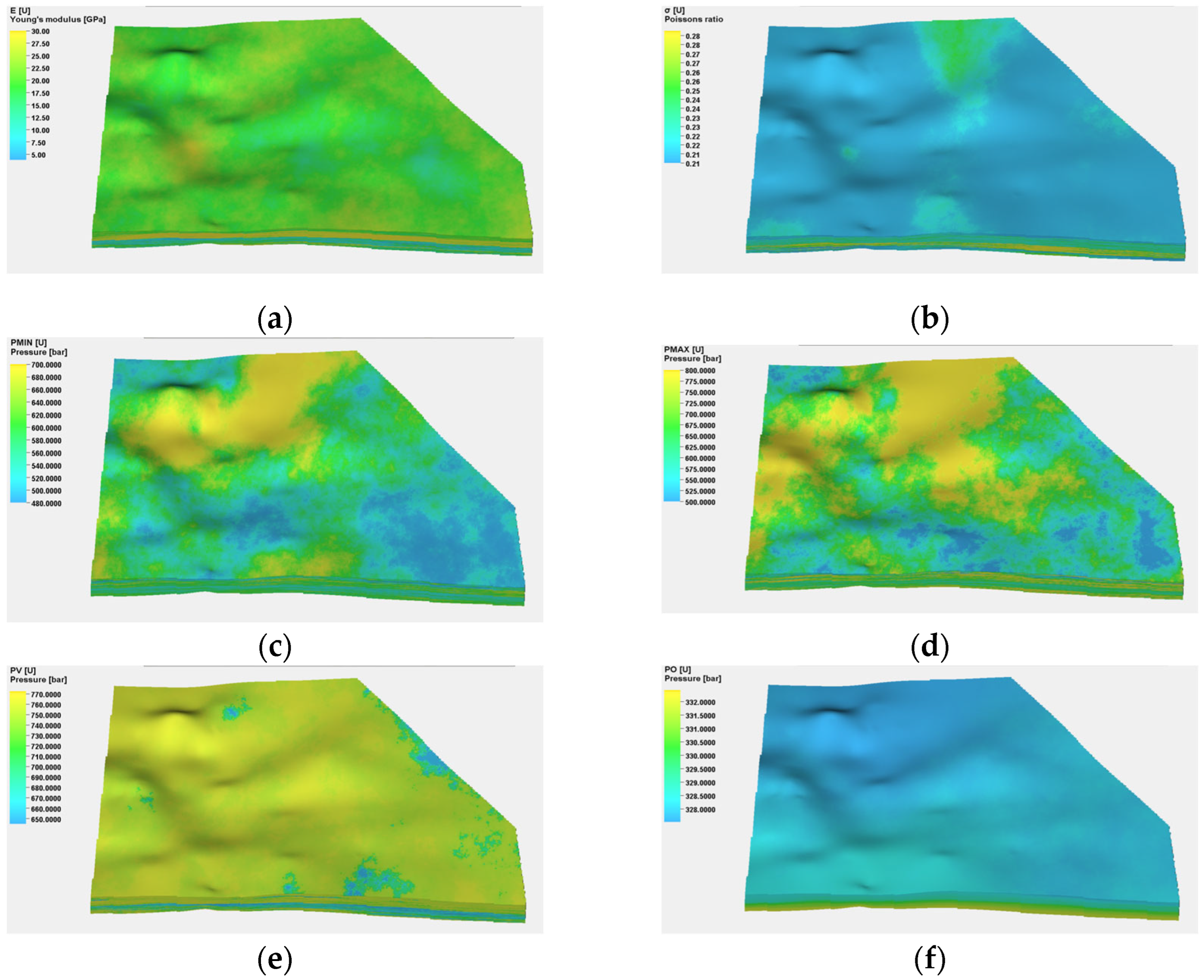
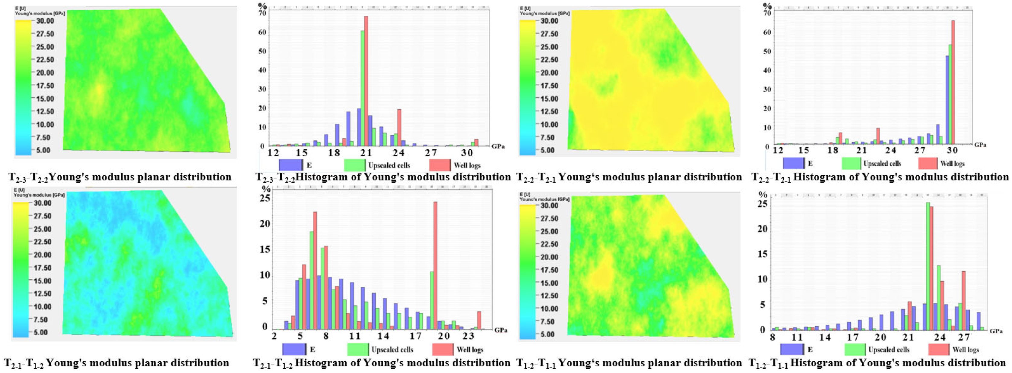
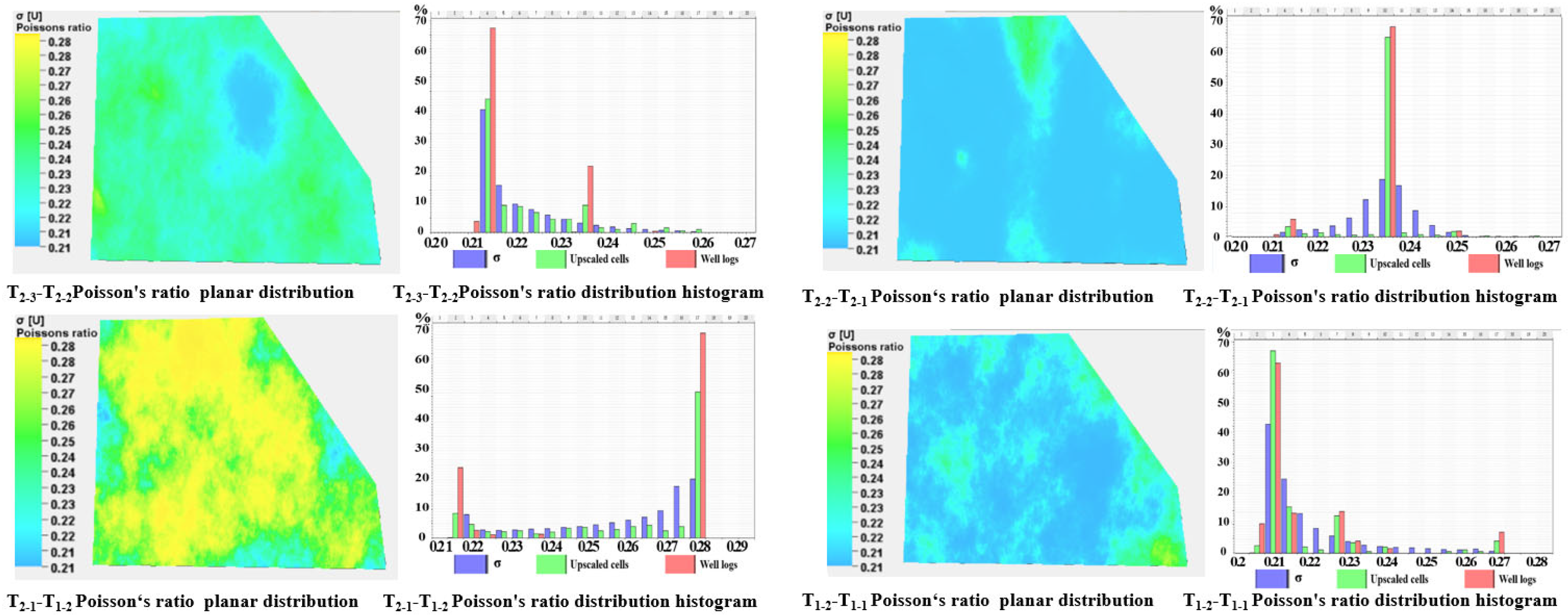
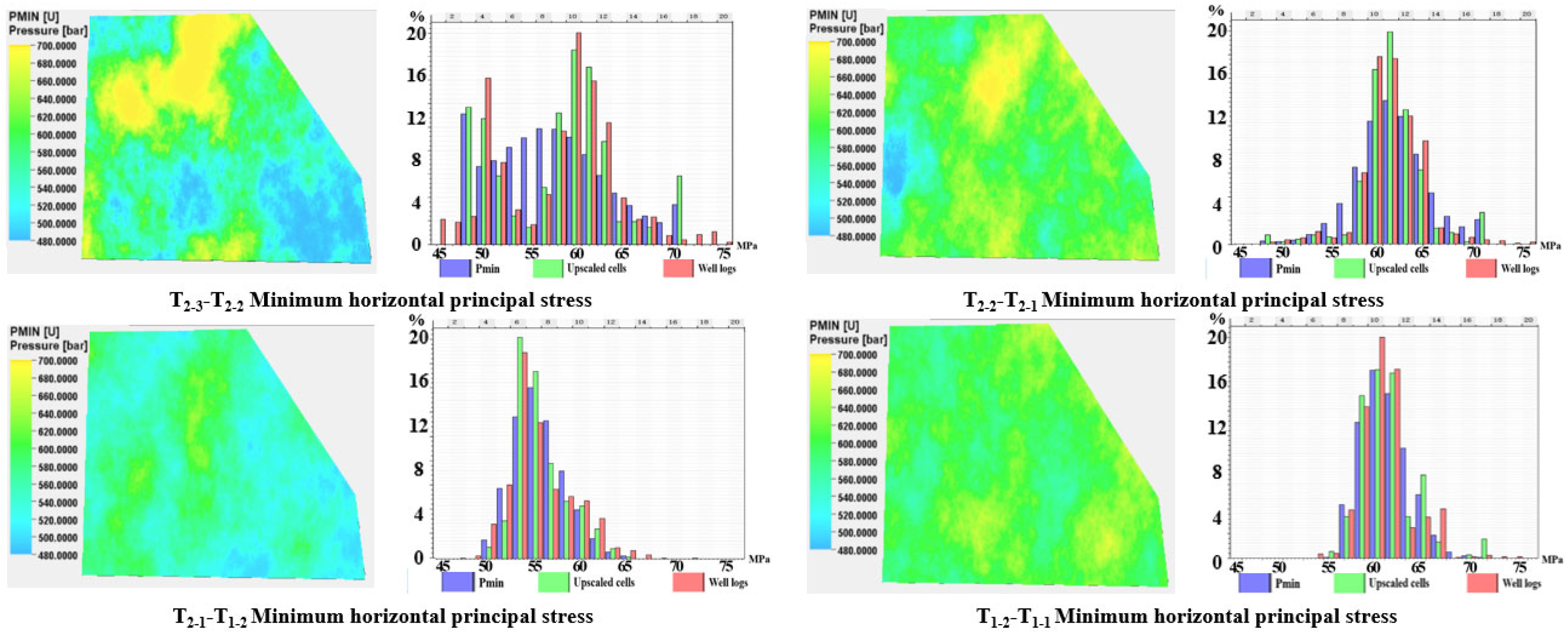
3.3. Rock Mechanics and Stress Modeling

Acoustic travel time logs are utilized to determine the rock mechanics and stress parameters of each well. This is performed using regression formulas for P-to-S wave conversion, empirical rock mechanics equations, and the deep coal-seam-applicable Ge model. New well logs were created to include Young’s modulus, Poisson’s ratio, and the minimum and maximum horizontal and vertical principal stresses. An average algorithm was applied, and the properties were discretized. Additionally, harmonic mean, facies-controlled, and sequential Gaussian simulation algorithms were employed to generate 3D geological property models for these parameters. The geological model of the rock mechanics and stresses in the target area is shown in Figure 7.

As shown in Figure 8, the Young’s modulus of the roof ranges from 14 GPa to 32 GPa, with a mean value of 30 GPa. The Young’s modulus of coal varies from 3 GPa to 12 GPa, averaging 7.5 GPa. The floor’s Young’s modulus spans from 10 GPa to 25 GPa, with a mean of 20 GPa.

As shown in Figure 9, the roof has a Poisson ratio of 0.21 to 0.28, with an average of 0.23. The coal has a Poisson ratio ranging from 0.26 to 0.29, averaging 0.28. The floor’s Poisson ratio varies from 0.2 to 0.26, with a mean of 0.21.

As shown in Figure 10, the minimum horizontal principal stress for the roof ranges from 48 MPa to 70 MPa, with an average of 61 MPa. For the coal seam, the minimum horizontal principal stress is between 49 MPa and 64 MPa, averaging at 53 MPa. The floor exhibits a minimum horizontal principal stress ranging from 55 MPa to 70 MPa, with an average of 59 MPa.

As shown in Figure 11, the maximum horizontal principal stress of the roof ranges from 50 MPa to 81 MPa, with an average value of 72 MPa. For the coal seam, the maximum horizontal principal stress varies from 56 MPa to 75 MPa, with a mean of 61 MPa. The floor exhibits a maximum horizontal principal stress that ranges from 61 MPa to 80 MPa, averaging 71 MPa.

As shown in Figure 12, the vertical principal stress of the roof and floor is approximately 75 MPa, while that of the coal seam is around 66 MPa. In the coal seam, the vertical stress (66 MPa) exceeds the maximum horizontal principal stress (61 MPa), which in turn is greater than the minimum horizontal principal stress (53 MPa). The difference between the horizontal stresses is about 8 MPa. Additionally, the stress difference among the coal seam, roof, and floor ranges from 8 to 12 MPa. The average pore pressure of the reservoir is 32.5 MPa. The pore pressure profile is shown in Figure 13.

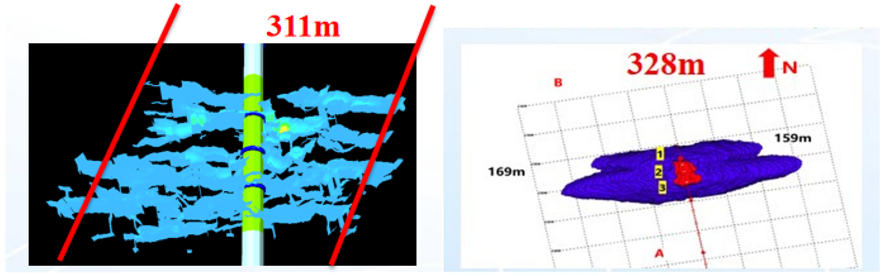
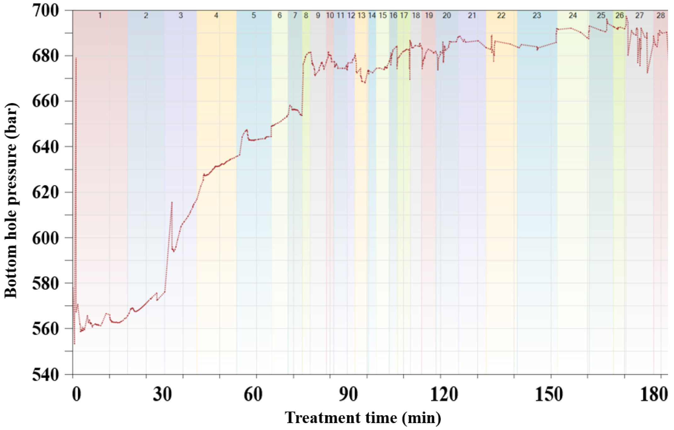
3.4. Establishment and Calibration of Hydraulic Fracturing Model for Deep Coal Reservoirs

Based on established 3D geological and stress field models, we developed a hydraulic fracturing model that takes into account natural fractures and coal seam cleats. The fracturing parameters and pumping program for Field X well were simulated for different azimuth fracture models. After adjusting for the loss coefficient of the fractures (including their length and height), we utilized the closest fracture network morphology as the natural fracture model for the healthy group area. Figure 14 compares the monitoring results of the fracturing fluid wavefront from well X with the results of numerical simulations. Figure 15 illustrates the construction pressure fitting of the established fracturing model using the construction parameters from well X, which aligns with the actual site conditions.

The geological parameters of the coal seam in the fracturing model are as follows: average Poisson’s ratio of 0.28, Young’s modulus of 3–9 GPa, minimum horizontal principal stress of 53 MPa, maximum horizontal principal stress of 60 MPa, and vertical principal stress of 65.5 MPa. The stress difference between Taiyi coal seam and roof is 11–13 MPa, and the stress difference between Taiyi coal seam and bottom plate is 8–10 MPa; the main drilling encounter rock facies is bright coal. The numerical simulation uses the Y well group, which has a total of four horizontal wells, of which the horizontal section length of Y1, Y3 and Y4 wells is 1000 m, the horizontal section length of Y2 well is 800 m, the well spacing of Y1 and Y2 wells is 4000 m, and the adjacent well spacing of the rest of the wells is 350 m. Figure 16 is a schematic diagram of the borehole trajectory of the well group.

4. Fracturing Parameter Optimization

Considering the influences of intersection fracture spacing, construction fluid volume, and construction displacement on fracture propagation under single well conditions and well group conditions, the above construction parameters were optimized by comparing the fracture propagation morphology, in situ stress field change, conductivity, fracture making volume, and other factors. The specific process is as follows: Firstly, according to the construction data of the site, the control variable method is used to simulate the law of mesh propagation and crack parameters under different inter-section seam spacing, and the optimal inter-segment seam spacing is optimized by comprehensively considering the seam network ripple area, channeling situation, stress interference, conductivity and seam volume value. Then, the optimized inter-segment seam spacing was replaced by the inter-segment seam spacing used in the on-site construction scheme, and then the control variable method was used to simulate the seam network expansion law under different construction fluid quantities to optimize the construction fluid volume. Finally, the optimized inter-segment joint spacing and liquid volume are replaced by the inter-segment joint spacing and liquid volume used in the on-site construction scheme, and the construction displacement is optimized according to the above process.

The construction parameters of the foundation are a section of 3 clusters: cluster spacing 20 m; each cluster perforation is 1 m, and the hole density is 16 rounds/m; phase angle 60°; the comprehensive sand ratio is 14%; the viscosity of fracturing fluid is 31 mPa.s; the single well simulation uses a perforated well section of 600 m (3720~4320 m) of Well Y1, and the gap spacing between the sections is 30–90 m. Construction fluid volume 2500–4500 m³; construction row 10–30 m³/min. The perforated sections of the well group were a 600 m horizontal section (3720~4320 m) of Well Y3 and a 600 m horizontal section (3670~4270 m) of Well Y4, and the gap spacing between sections was 30–90 m; construction fluid volume: 2500–4500 m³; the construction displacement is 10–30 m³/min. For the specific pumping procedure, please refer to the on-site construction data of Well X1.

4.1. Single Well Fracturing Parameter Optimization

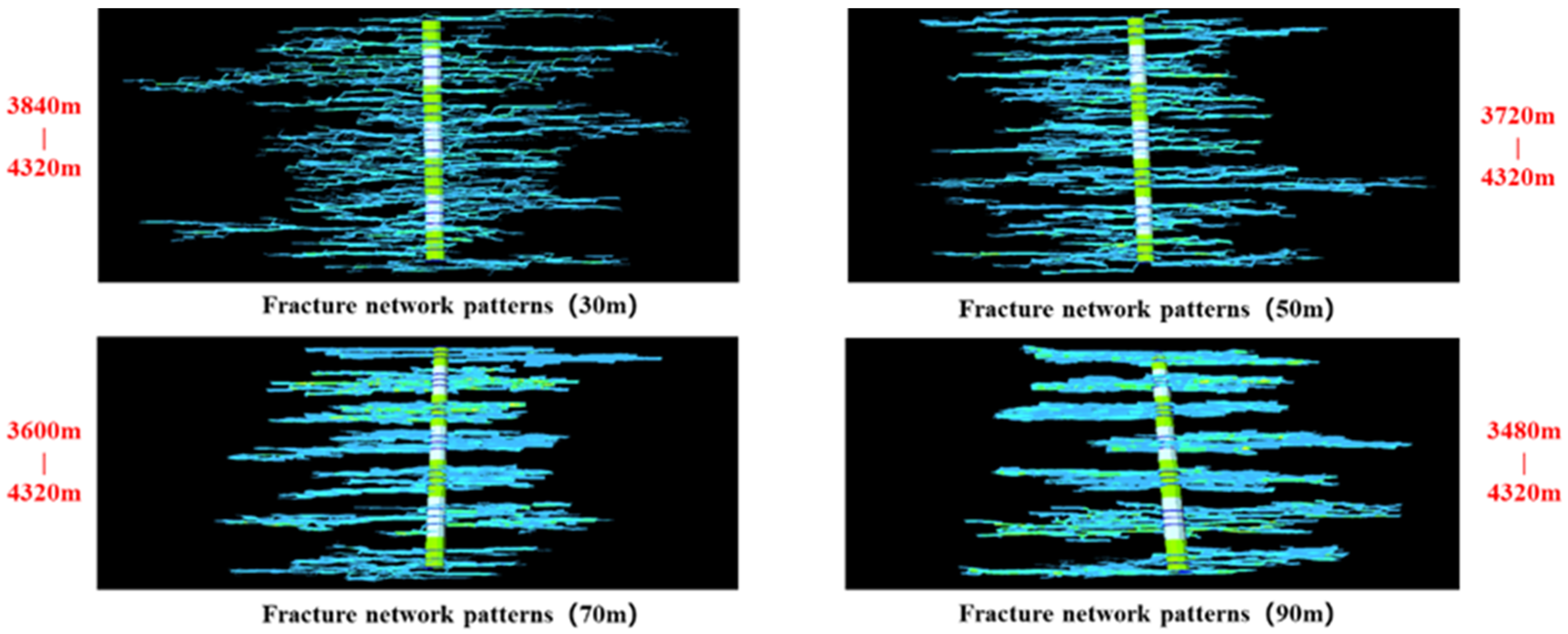
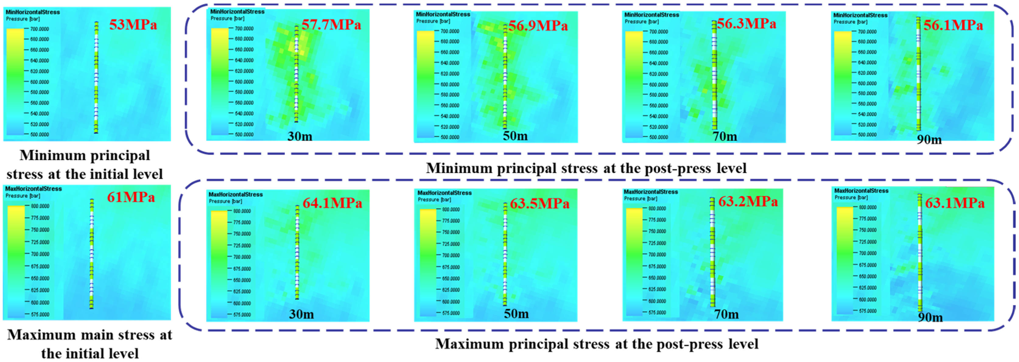
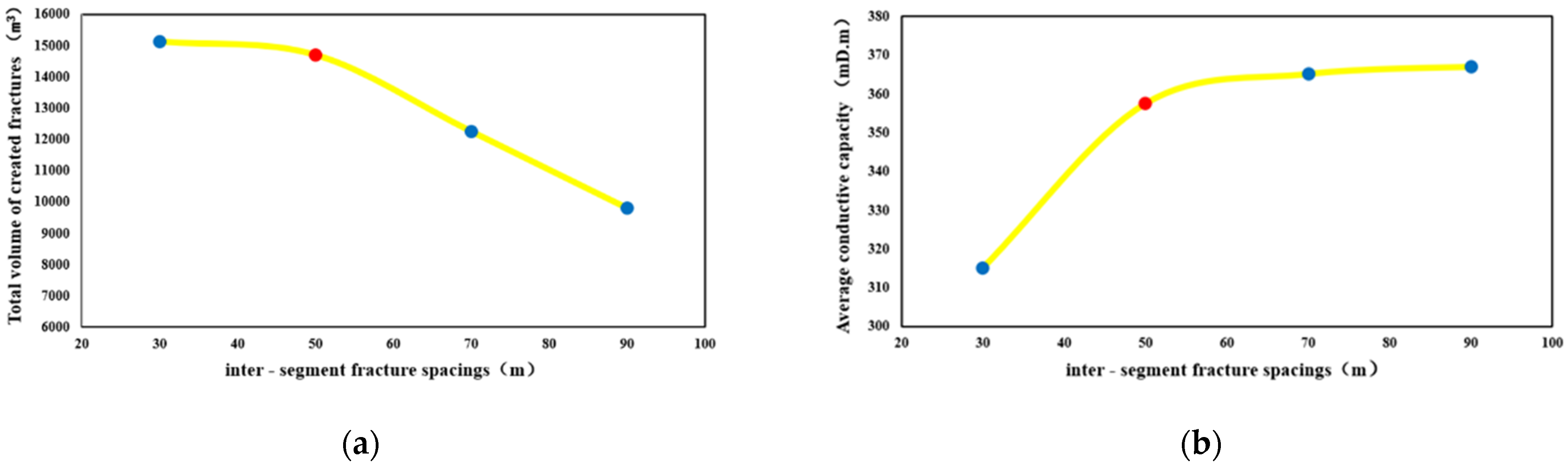
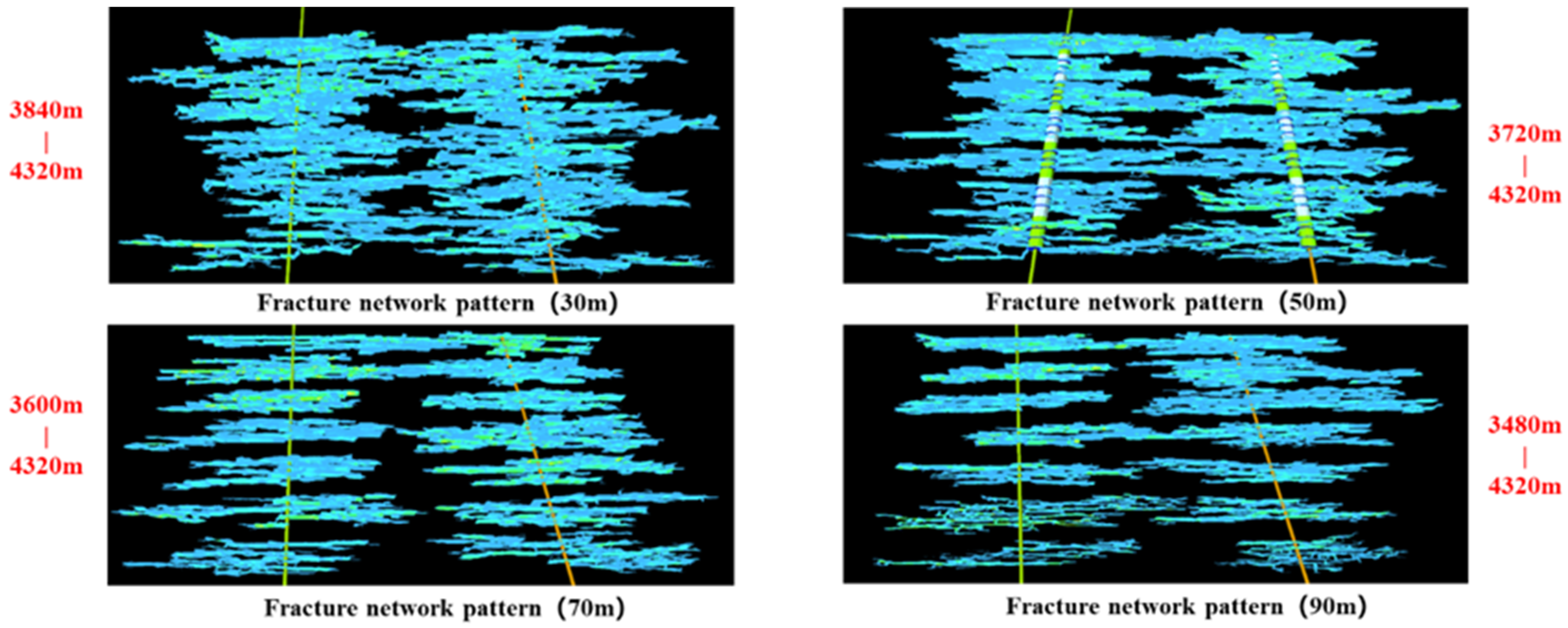
4.1.1. Inter-Stage Fracture Spacing

The inter-stage fracture spacing is the distance between the previous stage’s last perforation hole and the next stage’s first perforation hole. Figure 17 shows the fracture network morphology under different inter-stage fracture spacings. Results show that at 30 m spacing, inter-cluster and inter-stage interference are severe. At 50 m, there is almost no interference. No interference occurs when spacing exceeds 50 m, but the unfractured area between stages increases, leading to insufficient reservoir stimulation.

Figure 18 illustrates the variation of horizontal stress with different inter-stage fracture spacings. When the spacing is 30 m, there is a significant interference in horizontal stress. At 50 m spacing, the area of stress change is the largest, and the interference between stages is minimal. When the spacing exceeds 50 m, the interference in horizontal stress becomes weak. As the inter-stage fracture spacing increases, the rate of increase in horizontal stress decreases. After fracturing, the minimum horizontal principal stress increases by approximately 3.9 MPa, and the maximum horizontal principal stress increases by 2.5 MPa. Geological structure, rock properties, and fracturing parameters influence the variation in horizontal stress with inter-stage fracture spacing.

Figure 19 illustrates the total fracture volume and average conductivity curves for various inter-stage fracture spacings in a 1000 m horizontal coalbed methane well. When the spacing is less than 50 m, the total fracture volume experiences a slight decrease as the spacing increases, while the average conductivity per cluster improves. However, when the spacing exceeds 50 m, the total fracture volume drops significantly, and the average conductivity per cluster increases at a slower rate. These findings align with research on fracture conductivity in tight reservoirs, where factors such as stress closure and proppant properties have a significant impact on conductivity.

A comprehensive evaluation of fracture network morphology, total fracture volume, and conductivity under different inter-stage fracture spacings shows that around 50 m spacing yields the best results for the overall fracture network morphology, total fracture volume, and conductivity.

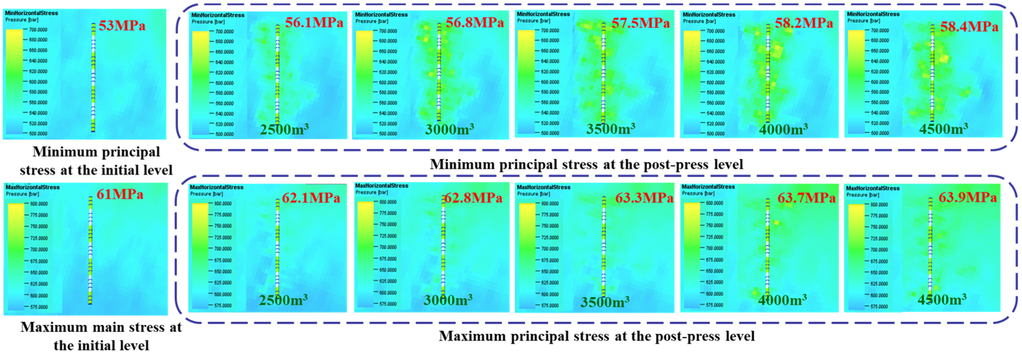
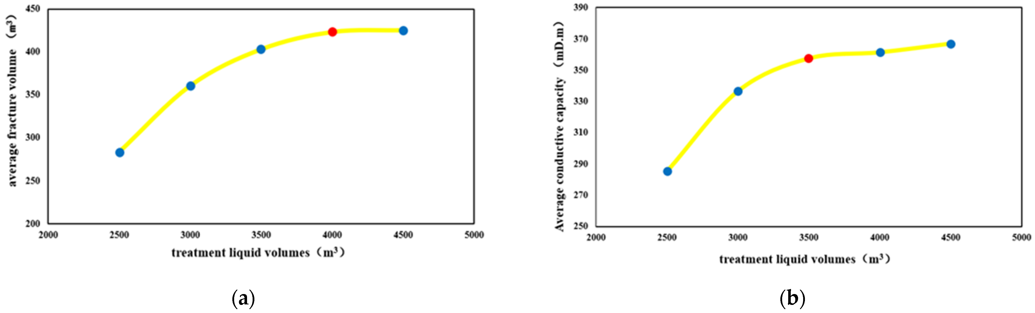
4.1.2. Fracturing Liquid Volume

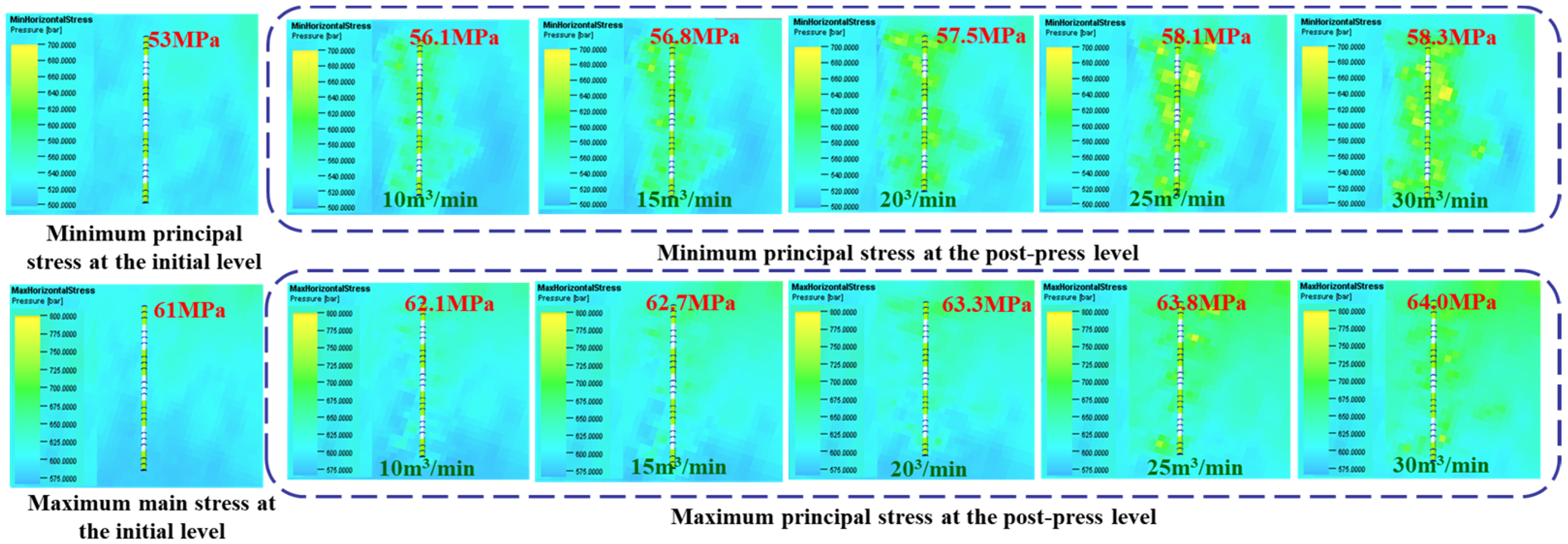
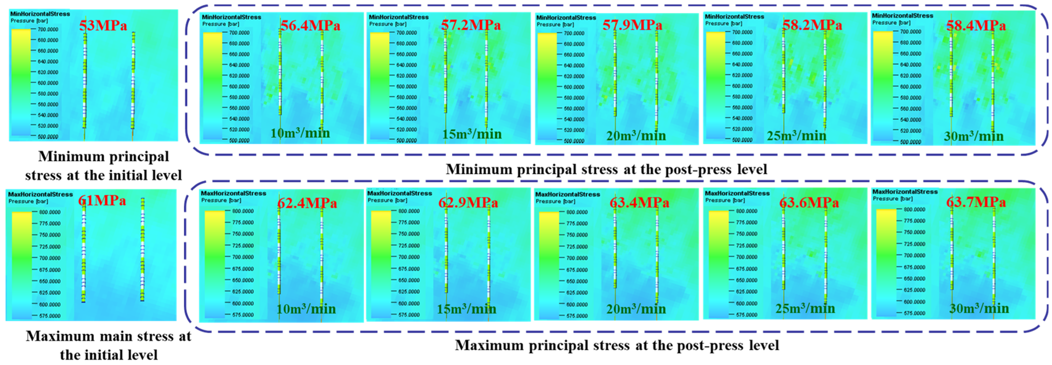
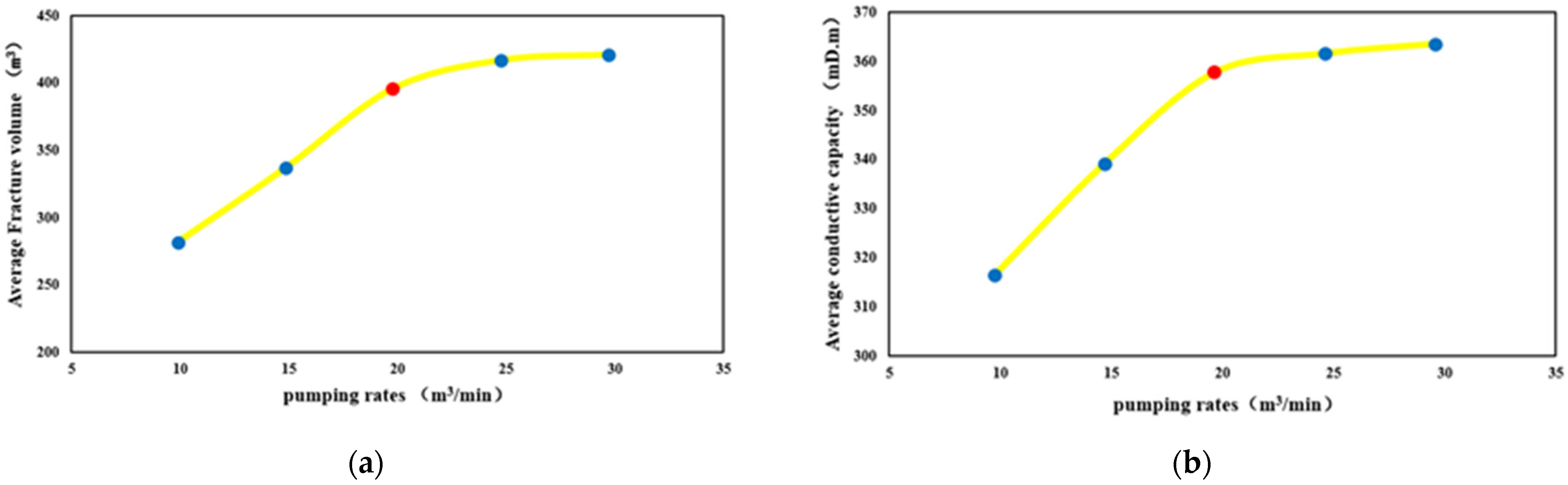
Figure 20 illustrates the fracture network morphology under different pumping liquid volumes. The volume of liquid used significantly impacts fracture network coverage. During the early fracturing stages, the stimulated volume increases rapidly with increasing liquid volume, then slows down after reaching a specific volume. For a coalbed methane horizontal well with a 50 m inter-stage fracture spacing and 18 m³/min discharge rate, the fracture coverage is low at 2500 m³ and 3000 m³ liquid volumes. The fracture coverage is better at 3500 m³ and 4000 m³, with minor inter-stage interference. At 4500 m³, the fracture coverage is high, but there is significant inter-stage interference. These findings are consistent with research indicating that excessive liquid volume can lead to rapid pressure drops and sustainability challenges in fracture networks.

Figure 21 shows the stress changes under different pumping liquid volumes. At 2500 m³ and 3000 m³ liquid volumes, the stress change area is small, with weak inter-stage and cluster interference, but there are still many unfractured areas. Stress increases with liquid volume. The stress change area is large at liquid volumes above 3500 m³, but there is substantial inter-well and inter-stage interference. Stress increases slowly with liquid volume. After fracturing, the minimum horizontal principal stress increased by about 4.5 MPa, and the maximum horizontal principal stress increased by about 2.3 MPa.

Figure 22 illustrates the relationship between total fracture volume and average conductivity across different pumping liquid volumes. When the liquid volume per stage is below 4000 m³, both the total fracture volume and average conductivity increase as the liquid volume rises. However, once the liquid volume per stage exceeds 4000 m³, while both the total fracture volume and average conductivity continue to increase, the rate of increase slows significantly.

A comprehensive evaluation of fracture network morphology, stress changes, total fracture volume, and conductivity under varying volumes of fracturing liquid indicates that approximately 3500–4000 m³ per stage yields optimal results for fracture network morphology and conductivity.

4.1.3. Pumping Rate

Figure 23 shows fracture network morphologies under different pumping rates. With an inter-stage fracture spacing of 50 m and a liquid volume of 4000 m³, fracture coverage is low at rates of 10–15 m³/min. At 20 m³/min, there is minor inter-stage interference and better fracture coverage. Fracture coverage is high at 25–30 m³/min, but there is significant inter-stage and cluster interference.

Figure 24 shows the stress changes under different pumping rates. When the pumping rate is below 20 m³/min, the area of stress change is small, with some unfractured regions remaining between stages. As the pumping rate increases, the stress change also increases. However, when the rate exceeds 20 m³/min, the area of stress change becomes significantly larger, leading to noticeable interference between stages, and the rate of stress change increases more slowly. After the fracturing process, the minimum horizontal principal stress increases by approximately 3.6 MPa, while the maximum horizontal principal stress rises by about 2.2 MPa.

Figure 25 illustrates the total fracturing volume and average conductivity at varying pumping rates. When the rate is below 22 m³/min, both volume and conductivity increase with the rate. Above 22 m³/min, the rate of increase in conductivity slows down.

A comprehensive evaluation of fracture network morphology, stress variation, and fracture volume and conductivity shows that the overall fracture network morphology and fracture parameter results are optimal at a pumping rate of around 20–22 m³/min.

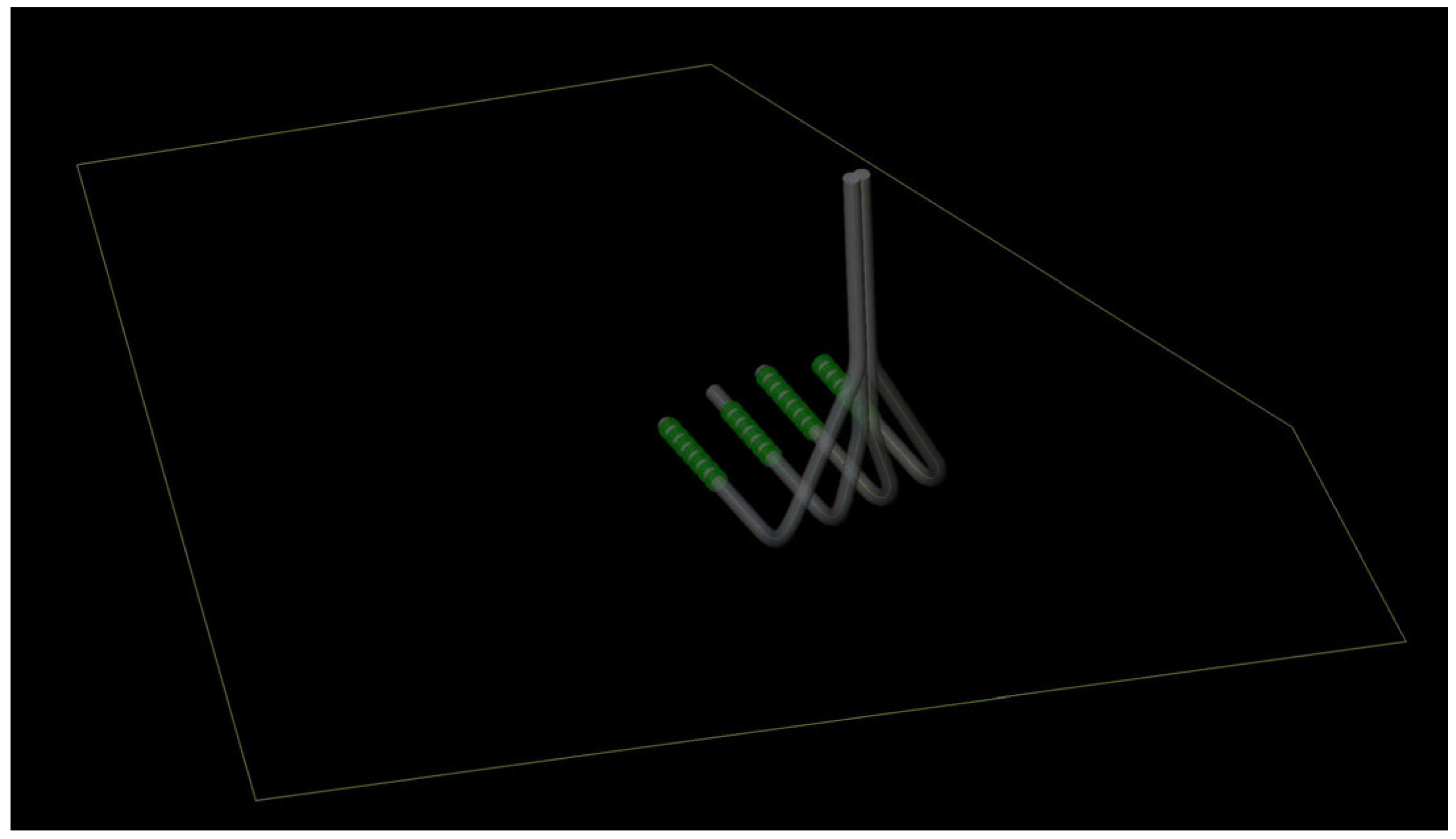
4.2. Well Group Fracturing Parameter Optimization

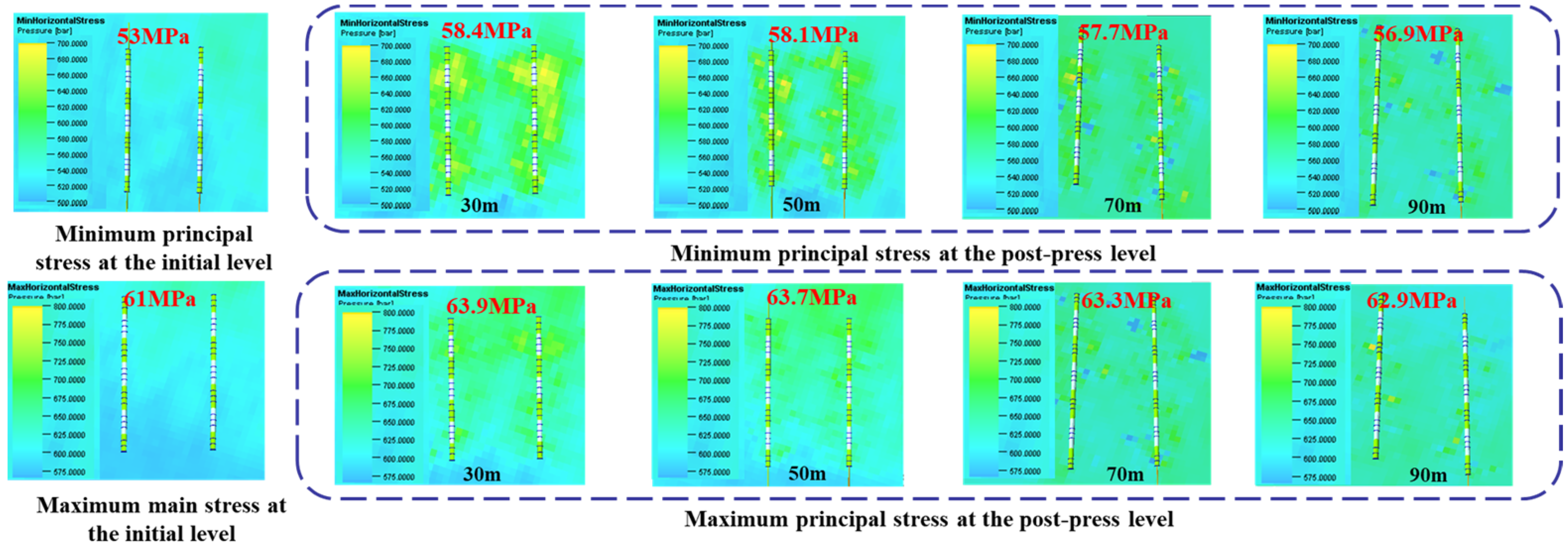
4.2.1. Inter-Stage Fracture Spacing

Figure 26 illustrates the morphology of the fracture network under various inter-stage fracture spacings, using a liquid volume of 3500 m³ and a discharge rate of 22 m³/min. At a spacing of 30 m, there is significant inter-cluster and inter-well interference. When the spacing is adjusted to 50 m, only minor inter-stage and inter-well interference is observed. However, when the spacing exceeds 70 m, inter-well interference is minimal, but this results in low fracture coverage and insufficient stimulation of the reservoir.

Figure 27 illustrates how stress varies with inter-stage fracture spacing. As the spacing increases, inter-stage interference decreases, leading to a reduced post-fracturing increase in stress. At 30 m of spacing, both inter-stage and inter-well stress interference are significant. At 50 m of spacing, the area of stress change is large, but inter-well interference becomes minimal. Beyond 50 m, the unfractured areas between stages and wells increase. After fracturing, the minimum horizontal principal stress rises by approximately 5 MPa, while the maximum horizontal principal stress increases by about 2.7 MPa.

Figure 28 illustrates the total fracture volume and average conductivity curves for varying inter-stage fracture spacings. When the spacing is less than 60 m, the total fracture volume decreases gradually as the spacing increases, while the average conductivity per cluster improves. However, when the spacing exceeds 60 m, the total fracture volume drops significantly, and the average conductivity per cluster increases at a slower rate.

A comprehensive evaluation of fracture network morphology, stress changes, total fracture volume, and conductivity shows that around 60 m inter-stage fracture spacing yields the best overall results for fracture network morphology, total fracture volume, and conductivity.

Based on the qualitative evaluation of the mesh morphology, the change of in situ stress, the total fracture volume and the quantitative evaluation of the conductive capacity under different intersection seam spacing, when the inter-section seam spacing is about 60 m, the results of the overall seam network morphology, total seam volume and conductive capacity are optimal.

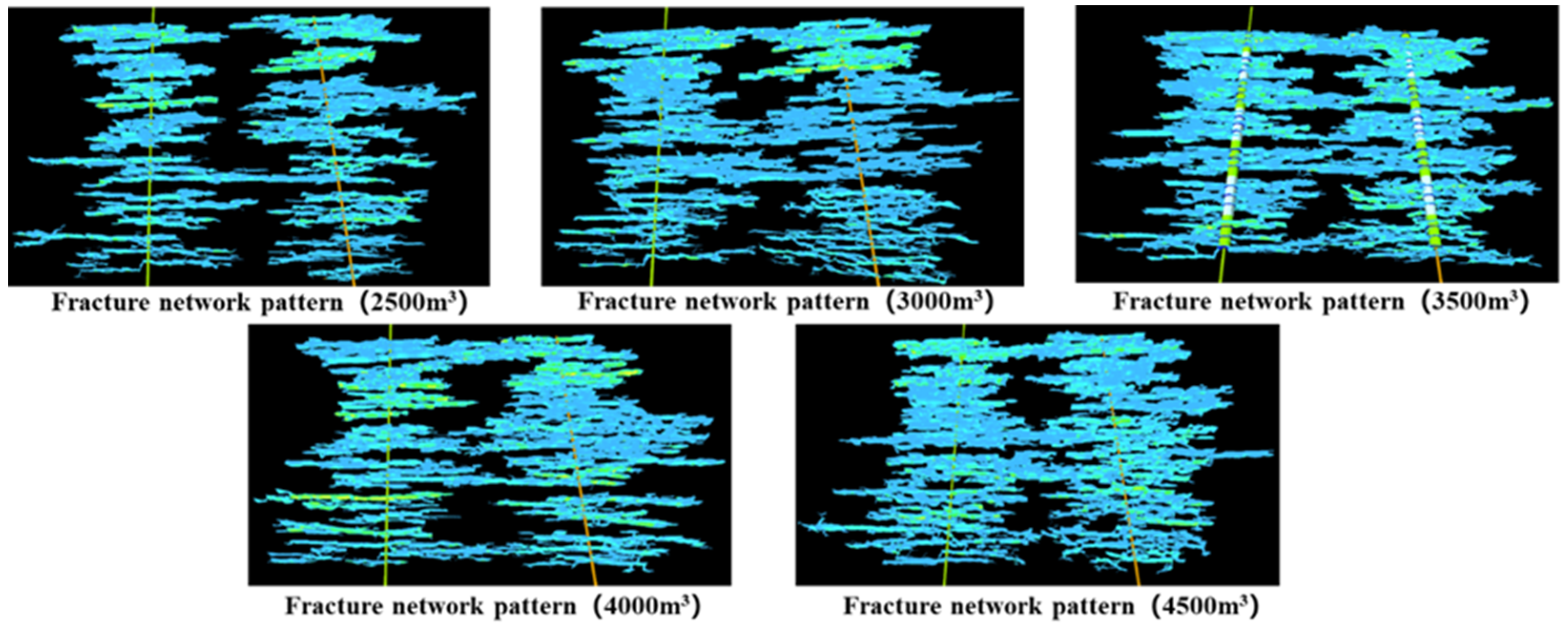
4.2.2. Fracturing Liquid Volume

Figure 29 presents the fracture network morphology under different fracturing liquid volumes with an inter-stage fracture spacing of 60 m and a 22 m³/min discharge rate. When the liquid volume is 2500–3000 m³, the fracture coverage between stages and wells is low. At 3500–4000 m³, coverage improves. At 4500 m³, coverage is high but with significant inter-stage and inter-well interference.

Figure 30 shows the stress variation under different fracturing liquid volumes. At 2500–3000 m³, the stress change area is small, with weak inter-well and inter-stage interference, but many unfractured areas exist. Stress increases with liquid volume. Above 3500 m³, the stress change area is large but with strong inter-well and inter-stage interference, and stress increases slowly with liquid volume. Post-fracturing, the minimum horizontal principal stress rises by about 5 MPa, and the maximum horizontal principal stress increases by 2.7 MPa.

Figure 31 illustrates the fracture volume and average conductivity at varying volumes of fracturing liquid. When the liquid volume per stage is less than 3500 m³, both fracture volume and conductivity increase with the volume. However, beyond 3500 m³, the rate of increase slows down.

A comprehensive evaluation of fracture network morphology, stress variation, fracture length, volume, and conductivity shows that around 3500 m³ per stage yields the best overall results.

Based on the qualitative evaluation of fracture network morphology, in situ stress change, and fracture length, fracture volume, and conductivity under different fracturing fluid volumes, when the single-stage fracturing fluid volume is about 3000–3500 m³, the overall fracture network morphology and conductivity are optimal.

4.2.3. Pumping Rate

Figure 32 shows the fracture network morphology under different pumping rates. With an inter-stage fracture spacing of 60 m, a liquid volume of 3500 m³ per stage, and pumping rates of 10–15 m³/min, fracture coverage between stages and wells is low. At 20 m³/min, there is minor inter-stage and inter-well interference and better fracture coverage. At 25–30 m³/min, fracture coverage is high but with significant inter-stage and inter-well interference.

Figure 33 illustrates the variations in stress under different pumping rates. Below a rate of 20 m³/min, the area experiencing stress changes is small, and there are some unfractured regions between the wells. As the pumping rate increases, the stress changes also increase. However, when the rate exceeds 20 m³/min, the area of stress change becomes significantly larger, leading to noticeable interference between the wells. In this case, the increase in stress changes occurs at a slower rate. After the fracturing process, the minimum horizontal principal stress increases by approximately 4 MPa, while the maximum horizontal principal stress rises by about 2.5 MPa.

Figure 34 presents the fracturing volume and average conductivity under different pumping rates. When the rate is below 20 m³/min, the volume and conductivity rise. Above 20 m³/min, the increase in conductivity slows down.

A comprehensive evaluation of fracture network morphology, stress variation, and fracture volume and conductivity shows that the overall fracture network morphology, fracture parameters, fracture volume, and conductivity are optimal at a pumping rate of around 18–20 m³/min.

4.3. Sensitivity Analysis

The optimization results of the construction parameters of the single well show that the construction parameters of Well Y1 are 50 m spacing, the construction fluid volume of the single section is 3500–4000 m³, the construction displacement is 20–22 m³/min, and the m0.ain seam length is about 315 m. The results of the optimization of the construction parameters of the well group show that the optimal construction parameters of wells Y3 and Y4 are 60 m spacing, 3000–3500 m³ of single-stage construction fluid, 18–20 m³/min, and about 303 m of main seam length.

Combined with the analysis of geological factors and engineering factors, it is concluded that the size of the fracture spacing between the sections is closely related to the degree of hydraulic fracture penetration, too large the fracture spacing between the sections will cause the hydraulic fractures to not be able to affect the middle area of the two adjacent sections, too small the spacing of the sections will cause the fracture network to be unable to extend outward due to the interference between the sections, and when the fracture spacing between the fracturing sections of the target coal seam reaches 50–60 m, the fracture network will be fully affected and the channeling phenomenon will be slight. When the amount of construction fluid is small, it is not conducive to the extension of hydraulic cracks and the formation of effective support joints, the larger the amount of construction fluid, the better the fracturing effect, but when the scale of construction fluid reaches a critical value, the increase of filtration loss and the phenomenon of channeling will lead to the continuous increase of scale and the effect of improving fracturing effect is not obvious, so when the construction fluid volume in the target area is 3000–4000 m³, a more ideal fracture length is formed. It also avoids the adverse effects of channeling and filtration, and saves costs. Although increasing the displacement is conducive to the expansion of the fracture network, the excessively high displacement may penetrate the roof and bottom plate of the reservoir, resulting in the obstruction of the expansion of the fracture network, so the fracturing effect is optimal when the current coal seam displacement reaches 18–22 m³/min.

5. Conclusions

(1) Based on the logging data of the well area, the three-dimensional natural fracture geology and in situ stress model of the well group area was calculated and established by modifying the calculation formula of deep coalbed methane mechanics and in situ stress, and the hydraulic fracturing simulation results of Well X were compared with the field fracture monitoring results. The results show that the mean value of Young’s modulus of the coal seam is 7.5 GPa, the average Poisson’s ratio is 0.28, the vertical principal stress is 66 MPa, the minimum horizontal principal stress is 53 MPa, the maximum horizontal principal stress is 61 MPa, and the stress difference between the top and bottom plate is 8–12 MPa.

(2) Based on the qualitative evaluation of the seam network morphology, the change of in situ stress, the quantitative evaluation of the fracture length, the volume of the fracture and the conductivity under different construction parameters, the results show that the optimal construction parameters of a single well are 50 m between sections, 3500–4000 m³ of construction fluid volume for a single section, 20–22 m³/min for construction displacement, and 315 m for the average main seam length.

(3) Based on the qualitative evaluation of the seam network morphology, the change of in situ stress, the quantitative evaluation of the fracture length, the fracture volume and the conductivity under different construction parameters, the results show that the optimal construction parameters are 60 m between sections when the well spacing is 350 m, the construction fluid volume of a single section is 3000–3500 m³, the construction displacement is 18–20 m³/min, and the average main seam length is 305 m. It can be seen that under the influence of stress shadow and fracture disturbance, the construction scale is smaller than that of a single well, and the fracture length is shorter.

(4) In the study area with an initial minimum horizontal principal stress of 53 MPa and a maximum of 57 MPa, the optimal parameters increase the single well’s minimum horizontal principal stress by 4.5 MPa and maximum by 2.3 MPa. The post-fracturing stress increase for good groups is more significant due to inter-well stress interference.

References

1. Pang, X.Q.; Jia, C.Z.; Wang, W.Y. Petroleum geology features and research developments of hydrocarbon accumulation in deep petroliferous basins. Pet. Sci. 2015, 12, 1–53. [Google Scholar] [CrossRef]
2. Xu, C.G.; Zhu, G.H.; Ji, H.Q. Exploration progress and reserve increase strategy of onshore natural gas of CNOOC. China Pet. Explor. 2024, 29, 32–46. [Google Scholar]
3. Zhang, Q.; Jiang, W.P.; Jiang, Z.B. Present situation and technical research progress of coalbed methane surface development in coal mining areas of China. Coal Geol. Explor. 2023, 51, 139–158. [Google Scholar]
4. Qing, S.R.; Cun, Z.; Guang, W. Hydraulic fracture initiation and propagation in deep coalbed methane reservoirs considering weak plane: CT scan testing. Gas Sci. Eng. 2024, 125, 205286. [Google Scholar]
5. Zhou, D.H.; Chen, G.; Chen, Z.L. Exploration and development progress, key evaluation parameters and prospect of deep CBM in China. Nat. Gas Ind. 2022, 42, 43–51. [Google Scholar]
6. Xie, H.P.; Gao, F.; Ju, Y. Research and exploration of deep rock mass mechanics. Chin. J. Rock Mech. Eng. 2015, 34, 2161–2178. [Google Scholar]
7. Xiong, D.; He, J.Y.; Ma, X.F. Fracturing simulation with different perforation positions atdeep coal seam and roof/floor rock—case study at the No.8 deep coal seam of a gas-field in the Ordos basin. J. China Coal Soc. 2024, 49, 4897–4914. [Google Scholar] [CrossRef]
8. Lei, N.Z. Predication and Stochastic Modeling of Coalbed Methane Reservoir Properties in Luling Well Field. Ph.D. Thesis, China University of Mining and Technology, Xuzhou, China, 2012. [Google Scholar]
9. Qu, L.C. Geological Modeling Technology and Application of Coalbed Methane. Ph.D. Thesis, China University of Geosciences (Beijing), Beijing, China, 2013. [Google Scholar]
10. Huai, Y.C.; Zhang, M.; Yang, L.W. 3D geological modeling of coalbed methane reservoirs based on facies control. J. Earth Sci. Environ. 2017, 39, 275–282. [Google Scholar]
11. Ma, P.H.; Shao, X.J.; Huo, M.Y. Geological modeling ideas and methods for coal reservoirs. Pet. Geol. Oilfield Dev. Daqing 2018, 39, 601–610. [Google Scholar]
12. Chen, B.; Tang, D.Z.; Zhang, Y.P. Logging inversion and 3D geological modeling of coal body structure. Coal Sci. Technol. 2019, 47, 88–94. [Google Scholar]
13. Liu, W.; Zhang, S.A.; Peng, C. Research on pressure drawdown characteristics during coalbed methane drainage. Coal Technol. 2019, 38, 18–21. [Google Scholar]
14. Li, Y.; Jiang, Z.B.; Liu, Y.H. Analysis of production characteristics of coalbed methane wells based on 3D geological modeling. Coal Mine Saf. 2020, 51, 190–194. [Google Scholar]
15. Lü, J.T.; Zhang, M.; Huai, Y.C. Wang Dianao Coal Reservoir Logging Analysis and Fine Geological Modeling Technology: A Case Study of Coalbed Methane Area in Surat Basin, Australia. J. China Coal Soc. 2020, 45, 1824–1834. [Google Scholar]
16. Zhou, Y.; Zhang, S.H.; Tang, S.H. 3D modeling of gas content in coalbed methane reservoirs. Coal Geol. Explor. 2020, 48, 96–103. [Google Scholar]
17. Xiang, L.W.; Jie, N.P.; Yi, J. Morphology and propagation of supercritical carbon dioxide-induced fractures in coal based on a non-destructive surface extraction method. Fuel 2025, 384, 133948. [Google Scholar]
18. An, Q.; Yang, F.; Yang, R.Y. Volume fracturing practice and understanding of deep coalbed methane in the Shenfu area, Ordos Basin. J. Coal Sci. Eng. 2024, 49, 2376–2393. [Google Scholar]
19. Li, B.; Yang, F.; Zhang, H.J. Research on efficient development technology of deep coalbed methane in the Shenfu area. Coal Geol. Explor. 2024, 52, 57–68. [Google Scholar]
20. Yang, F.; Li, B.; Wang, Q.J. Large-scale limit volume fracturing technology for deep coalbed methane horizontal wells. Pet. Explor. Dev. 2024, 51, 389–398. [Google Scholar]
21. Liu, X. Comparison of fracture network morphology in coal reservoirs under different fracturing scales. Reserv. Eval. Dev. 2024, 14, 510–518. [Google Scholar]
22. Xiong, X.Y.; Zhen, H.B.; Li, S.G. Multi-round turn fracturing technology and application for deep coalbed methane in the Da Ning-Ji County area. Coal Geol. Explor. 2024, 52, 147–160. [Google Scholar]
23. Zhong, Z.T.; Zhuang, X.; Yu, H.W. Numerical simulation of fracture propagation in deep coalseam reservoirs. Energy Sci. Eng. 2023, 11, 3559–3574. [Google Scholar]
24. Zhi, H.Z.; Tian, Y.W.; Jian, C.G. Study on the Spatial and Temporal Evolution Law of Large-Size Fracture Propagation in Deep Coalbed Based on Acoustic Emission Technology. Rock Mech. Rock Eng. 2025, 58, 3799–3814. [Google Scholar] [CrossRef]
Figure 1. Construction model diagram.
Processes 13 01699 g001
Figure 2. Reservoir lithofacies profile.
Processes 13 01699 g002
Figure 3. Geological model of porosity for the target block.
Processes 13 01699 g003
Figure 4. Geological model of permeability for the target block.
Processes 13 01699 g004
Figure 5. Histogram of porosity distribution for each small layer in the well group area.
Processes 13 01699 g005
Figure 6. Histogram of permeability distribution for each small layer in the well group area.
Processes 13 01699 g006
Figure 7. Geological model of rock mechanics and stress for the target area. (a) Young’s modulus; (b) Poisson’s ratio; (c) Minimum horizontal principal stress; (d) Maximum horizontal principal stress; (e) Vertical principal stress; (f) Pore pressure.
Processes 13 01699 g007
Figure 8. Distribution map of Young’s modulus for each small layer.
Processes 13 01699 g008
Figure 9. Distribution map of Poisson’s ratio for each small layer.
Processes 13 01699 g009
Figure 10. Distribution map of minimum horizontal principal stress for each small layer.
Processes 13 01699 g010
Figure 11. Distribution map of maximum horizontal principal stress for each small layer.
Processes 13 01699 g011
Figure 12. Vertical principal stress profile.
Processes 13 01699 g012
Figure 13. Pore pressure profile.
Processes 13 01699 g013
Figure 14. Comparison chart of X well’s fracturing fluid wave monitoring results and numerical simulation results.
Processes 13 01699 g014
Figure 15. Numerical simulation of the construction pressure curve of a well.
Processes 13 01699 g015
Figure 16. Schematic diagram of the borehole trajectory of the Y well group.
Processes 13 01699 g016
Figure 17. Fracture network patterns under different inter-segment fracture spacings.
Processes 13 01699 g017
Figure 18. Ground stress variations under different inter-segment fracture spacings.
Processes 13 01699 g018
Figure 19. Total fracture volume and average conductive capacity under different inter-segment fracture spacings. (a) Total volume of created fractures under different inter-segment fracture spacings; (b) Average conductive capacity under different inter-segment fracture spacings.
Processes 13 01699 g019
Figure 20. Fracture network patterns under different pumping liquid volumes.
Processes 13 01699 g020
Figure 21. Formation stress variations under different treatment liquid volumes.
Processes 13 01699 g021
Figure 22. Fracture volume and average conductive capacity under different treatment liquid volumes. (a) Total fracture volume under different treatment liquid volumes; (b) Average conductive capacity under different treatment liquid volumes.
Processes 13 01699 g022
Figure 23. Fracture network patterns under different pumping rates.
Processes 13 01699 g023
Figure 24. Formation stress variations under different pumping rates.
Processes 13 01699 g024
Figure 25. Total fracture volume and average conductive capacity under different treatment liquid volumes. (a) Fracture volume under different pumping rates; (b) Average conductive capacity under different pumping rates.
Processes 13 01699 g025
Figure 26. Fracture network patterns under different inter-segment fracture spacings.
Processes 13 01699 g026
Figure 27. Formation stress variations under different inter-segment fracture spacings.
Processes 13 01699 g027
Figure 28. Curve chart of total fracture volume and average conductive capacity under different inter-segment fracture spacings. (a) Total fracture volume under different inter-segment fracture spacings; (b) Average conductive capacity under different inter-segment fracture spacings.
Processes 13 01699 g028
Figure 29. Fracture network patterns under different treatment liquid volumes.
Processes 13 01699 g029
Figure 30. Formation stress variations under different treatment liquid volumes.
Processes 13 01699 g030
Figure 31. Total fracture volume and average conductive capacity under different treatment liquid volumes. (a) Average fracture volume per cluster under different liquid volumes; (b) Average conductive capacity under different liquid volumes.
Processes 13 01699 g031
Figure 32. Fracture network patterns under different pumping rates.
Processes 13 01699 g032
Figure 33. Formation stress variations under different pumping rates.
Processes 13 01699 g033
Figure 34. Total fracture volume and average conductive capacity under different pumping rates. (a) Average fracture volume under different pumping rates; (b) Average conductive capacity under different pumping rates.
Processes 13 01699 g034