Analyzing the Impact of Orifice Size and Retention Time in Private Tanks on Water Quality Indicators in Distribution Networks

Abstract

Chlorine decay in water distribution networks is significantly affected by the presence of private storage tanks, particularly due to the orifice size and retention time, which influence both hydraulic flow behavior and water residence time. This study introduces a novel simulation framework that integrates pressure-driven analysis with a first-order kinetic model for chlorine decay, implemented using the WQnetXL tool and validated through simulations in EPANET. Two schematic models, including a real-world case from Dubai, were analyzed under varying orifice sizes and retention times. Results show that larger orifices lead to higher initial chlorine concentrations during tank filling due to increased flow rates, but result in a rapid decline in chlorine levels once the tanks reach full capacity. In contrast, smaller orifices maintain more stable chlorine concentrations over time due to prolonged inflow durations. Extended retention times further delay tank filling and sustain higher chlorine levels until the system transitions to behavior typical of demand-driven analysis. A reliability assessment of the Dubai case study indicated that incorporating private tanks can result in deviations in chlorine concentration of up to 30 percent compared to conventional models. This approach addresses a key gap in conventional network modeling by quantifying the influence of decentralized storage on disinfection effectiveness and network reliability.

1. Introduction

Water quality analysis is essential for evaluating a network’s ability to deliver clean water. This is done to avoid prolonged retention times within the network system, which can increase the water age and compromise quality. As such, chlorine is added to the effluent of the water treatment plant to ensure that no microorganisms are produced on the pipe’s walls and that water remains drinkable for the end user [1]. However, chlorine concentration varies as it reacts with the pipe walls. Therefore, associated water quality models that perform first-order decay equations are used to observe the network’s performance and whether it can maintain a set quantity of chlorine concentration prescribed by the Code of Practice [1,2,3,4,5].

Generally, to assess the performance of water distribution networks (WDNs), a certain value of known chlorine concentration is added to the reservoir of the network model, and based on the steady-state analysis, the chlorine concentration is calculated in the rest of the components using the Lagrangian Algorithm. This is based on fluid movement, which plays a vital role in the overall reaction of chlorine particles with the walls of the pipes. The concentration of chlorine changes over time based on the reaction of water parcels within the system using decay equations. Since integrating private tanks can affect the flow, it is important to analyze their effect on the chlorine concentration within the system and assess whether it remains under the prescribed threshold when associated with different orifice inlets and retention times.

Summary of the Literature

Based on the history of water quality modelling, many models have been developed that simulate the chlorine concentration in the nodes that decay over time as the water spreads into the network. The basis of modelling chlorine concentration comes from the algorithm that can solve the convenient transport problem in WDNs. Most researchers have worked on two techniques to evaluate concentration during water transport: steady-state analysis [6,7,8,9,10,11,12,13] and dynamic mathematical modelling [12,14,15]. Both of these techniques have shown different levels of success based on their capabilities, especially in the work of Liou and Kroon [15]. Their study introduced an algorithm known as the Lagrangian Time Driven Method (TDM).

In steady-state analysis, models use the law of conservation of mass to obtain the concentration distribution of the containment parcel that occurs once the WDN has approached the hydraulic equilibrium [12]. On the other hand, dynamic mathematical modelling is based on a system simulation approach to obtain the motion and progress of the containments under variable demand, continuous supply, and hydraulic conditions [12]. When comparing the two approaches, dynamic modelling tends to perform better because the system of WDN is based on the continuous process of water being supplied at every time interval. Therefore, dynamic modelling shows a more accurate and realistic representation of the time-varying interaction of hydraulic behavior and water quality.

Over the years, more research has been conducted to improve the limitations of dynamic modelling, including limitations such as long computational time, difficulty obtaining detailed network components, and model memory requirements. These problems were seen largely in networks with relatively long pipes with low velocities, which resulted in a loss of accuracy. As such, emphasis was placed on finding a more robust and efficient method.

To this end, the work of Boulos et al. [2] focused on employing a much more rigorous system simulation approach. The study derived the Lagrangian Event Driven Method (EDM) technique, which allows the network to simulate the containment–transport process based on the distribution system activities. The main merit of this method was that it allowed the dynamic modelling to become less sensitive to the structure of the network, along with decreased computational memory and system requirements. Later on, Boulos et al. [2] provided an extension for this method, which allowed EDM to handle time-varying hydraulic conditions by adopting a one-dimensional transport model that mixes the materials completely and instantaneously. Similarly, another study by Mau et al. [3] proposed a Linear Compartment Model (LCM) algorithm formulated analytically from the continuity and mass balance principles. This method also accounts for affective transport, the mixing process between the materials, and kinetic reactions by placing a decay coefficient.

The decay coefficient calculates the rate of pipe wall decay based on the difference in chlorine concentration between two points and estimates the water travel time between those two points. These decay rates are determined based on laboratory experiments that aim to reduce errors. First-order decay rate equations are affected by several factors, including pipe materials [16], initial chlorine concentration, pipe corrosion [17], and biofilm [18]. A review of these factors was investigated by Hallam et al. [4], who confirmed the influence of these factors in the actual water distribution networks.

As computational software improved, more researchers focused on water quality reliability. These indicators use a fraction of delivered quality to assess a network based on the simulation runs that kept the supplied concentration below the threshold [19]. Moreover, the same concept was applied to modelling the reliability of chlorine concentration, which is the ratio of days the residual fulfils the standards required for chlorine to the total number of days in the simulation [20]. Later, booster station operation was introduced to minimize the chlorine injection quantity [20,21,22]. Wang et al. [23] found the factors that affect the chlorine injection to WDNs by obtaining a chlorine decay coefficient in individual pipes in a network. This further validated that these coefficient values can be generalized to similar characteristics. Overall, modelling chlorine decay requires understanding the system and properly calibrating and validating tools for hydraulic modelling. This also includes accurate values for the kinetic constants required for the decay modelling. Therefore, such a technique was adopted in EPANET, which has a predefined set of water qualities. This allowed us to model chlorine decay based on a decay coefficient from the pipe wall and bulk composition.

In many types of research, the EPANET modelling tool was extended to water quality reliability for different real-time networks and extreme cases such as COVID-19. The methodology would often remain the same in these cases. However, the unique condition of each site with different decay constants, bulk decay rates, and calibration showed unique solutions for each case. For instance, research from Garcia-Avila et al. [1] has demonstrated that 45% of the nodal junctions in Azogues, Ecuador’s water network failed to comply with the Ecuadorian standards during the pandemic. This was due to a rise in network demand, which led to changes in flow and velocities that eventually affected the network’s bulk and wall decay coefficient. As such, the behavior of the network differentiated from the intended scenarios. This sudden change in demand also encouraged other tools for measuring water quality based on the risk index of disease occurrence [1]. Another instance took place in the city of Mohammedia, Morocco, where a study conducted by Belcaid et al. in 2023 [24] analyzed the city’s WDN using chlorine decay modelling in EPANET to optimize the dosage of chlorine concentration by identifying the chemical components present in the network. Finally, the 2023 study by Giustolisi et al. [25] developed a solving tool known as “WQnetXL” that allows unlimited water parcels to be simulated in low-velocity conditions during water quality analysis using the Lagrangian approach. Their study allows the network to be simulated efficiently based on the memory of the computational system. The validity of these models was verified by field research studies such as the tracer-based measurement, although more emphasis on calibration was required to ensure higher accuracy is obtained from the water-based simulation tools [26,27].

Therefore, since many factors impact water quality modelling, any changes in the network’s hydraulic behavior can affect chlorine’s containment–transport process. Since it is already established that the integration of private tanks affects the flow and pressure of the network system, the present study observes the impact on chlorine concentration of the network for different orifice sizes and retention times when compared to the standard chlorine values proposed by the regulatory authority. As such, it would demonstrate the water quality reliability of the network.

Thus, this study addresses a significant gap in existing chlorine decay modelling by integrating private storage tanks and pressure-driven analysis (PDA) into a dynamic simulation framework using WQnetXL. While past studies have evaluated chlorine decay in standard looped networks, the unique influence of intermittent supply systems with decentralized storage has not been extensively explored.

By simulating water quality using Extended Period Simulation (EPS) and first-order kinetic equations in WQnetXL and validating outcomes against EPANET’s chlorine decay model, this research offers a robust dual-model verification. The novel use of variable inflow curves derived from different orifice sizes and retention times within both platforms allows for a more realistic assessment of chlorine decay in networks with household-level tanks. This dual-layer modeling approach captures both hydraulic dynamics and water quality interactions more accurately, especially under non-ideal flow conditions.

2. Materials and Methods

2.1. Demand-Driven Analysis (DDA) vs. Pressure-Driven Analysis (PDA)

Hydraulic demand-driven analysis (DDA) assumes that the full consumer demand is always satisfied at each node in a water distribution network, regardless of the actual pressure available. It is a widely used and computationally efficient method, especially under normal operating conditions with adequate system pressure. DDA is commonly implemented in hydraulic simulation tools like EPANET (https://www.epa.gov/water-research/epanet, accessed on 21 May 2025), where it uses fixed demand values in the mass and energy balance equations to compute flows and pressures. However, this method cannot account for pressure-deficient scenarios or interruptions in supply, which limits its applicability in complex or non-ideal situations.

On the other hand, pressure-driven analysis (PDA) provides a more realistic approach by linking nodal outflows directly to available pressure at each junction. It allows demand to vary from zero up to the desired level depending on the system’s hydraulic state, making it suitable for abnormal conditions such as pipe bursts, leakages, or low-pressure zones. Importantly, modelling private storage tanks in water distribution networks requires the use of PDA, as tank filling and emptying processes depend on pressure-dependent inflow and outflow rates. Since storage tanks interact dynamically with the network based on local pressure and volume, the fixed-demand assumptions used in DDA would not capture their behavior accurately.

2.2. Modelling with Integrated Private Tanks

To simulate a water distribution network (WDN) with local storage, the system’s hydraulic behavior is modelled using momentum and continuity equations expressed in matrix form, as shown in Equation (1) [28].

$$\begin{array}{ccc}{\mathrm{A}}_{pp}\left(t\right){\mathrm{Q}}_p\left(t\right)+{\mathrm{A}}_{pn}{\mathrm{H}}_n\left(t\right)& =& -{\mathrm{A}}_{p0}{\mathrm{H}}_0\left(t\right)\\ {\mathrm{A}}_{np}{\mathrm{Q}}_p\left(t\right)-{\displaystyle \frac{{\mathrm{V}}_n\left(t,{\mathrm{H}}_n\left(t\right)\right)}{\Delta T}}& =& 0_n\end{array}$$

(1)

In this formulation, Q_p(t) is the vector of unknown pipe flows, H_n(t) represents the unknown nodal heads, H₀(t) represents the known heads (e.g., reservoirs), and V_n(t,H_n(t)) is the vector of total outflows during time step ΔT. The matrices A_pn, A_np, and A_p0 represent the network topology and relate links to nodes.

The second half of Equation (1) captures the mass balance at the nodes, where V_n = d_n∙$∆$T, and d_n represents pressure-dependent demands. These demands are broken down in Equation (2) into five components as follows:

$${\mathrm{V}}_n\left(t,{\mathrm{H}}_n\left(t\right)\right)={\mathrm{V}}_n^{cons}\left(t,{\mathrm{H}}_n\left(t\right)\right)+{\mathrm{V}}_n^{priv-tank}\left(t,{\mathrm{H}}_n\left(t\right)\right)+{\mathrm{V}}_n^{orif}\left(t,{\mathrm{H}}_n\left(t\right)\right)+{\mathrm{V}}_n^{tank}\left(t,{\mathrm{H}}_n\left(t\right)\right)+{\mathrm{V}}_n^{leak}\left(t,{\mathrm{H}}_n\left(t\right)\right)$$

(2)

where:

• V_n^cons (t, H_n(t)) denotes consumer demand, delivered fully if pressure meets minimum service levels; otherwise, calculated using Torricelli’s law.
• V_n^priv-tank (t, H_n(t)) denotes the volume flowing into private tanks, depending on tank status and nodal pressure [29].
• V_n^orif (t, H_n(t)) denotes the flow rate through free orifices like hydrants or pipe bursts, either known or pressure-dependent.
• V_n^tank (t, H_n(t)) denotes the volume flowing into or out of urban tanks, linked to system-wide water balance.
• V_n^leak (t, H_n(t)) denotes leakage from the network, modelled as pressure-dependent outflows due to infrastructure flaws (e.g., cracks, joints).

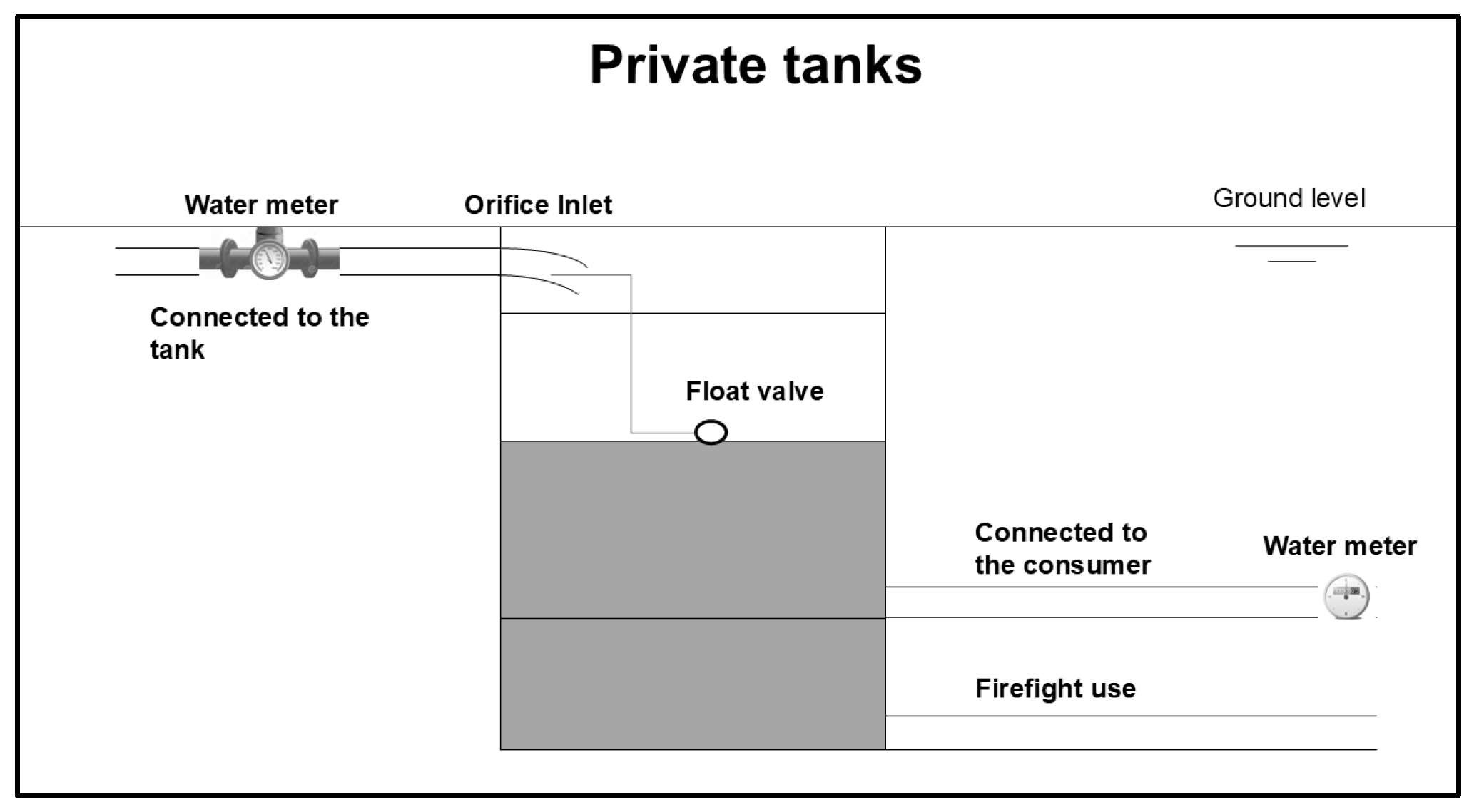
2.3. The Setup of Private Tanks

Under the Dubai Electricity and Water Authority’s (DEWA) regulations, every WDN connection must include a private storage tank sized to meet 24 h of consumption so that the supply remains uninterrupted during maintenance. In this study, private tanks were installed at each junction and sized according to DEWA’s 24-h demand standards, with retention intervals of 6, 12, 18, and 24 h evaluated [30]. Although water is pumped from these underground tanks up to rooftop tanks in practice, only the underground tank outlet is modelled here. A locally derived water demand profile was applied to all residential nodes, and the dynamics of tank filling and emptying were incorporated using a pressure-driven approach as shown in Figure 1 [31].

Each tank receives flow through a small diameter orifice, which is a short pipe whose effective area varies with the stored volume and directly links to the network junction. Orifices are typically located at the tank’s top, defining the junction’s elevation head. Their diameters range from 2 cm to 10 cm depending on local pressure and demand, and float valves govern orifice opening and closing in response to the tank’s water level based on the best practice from developers.

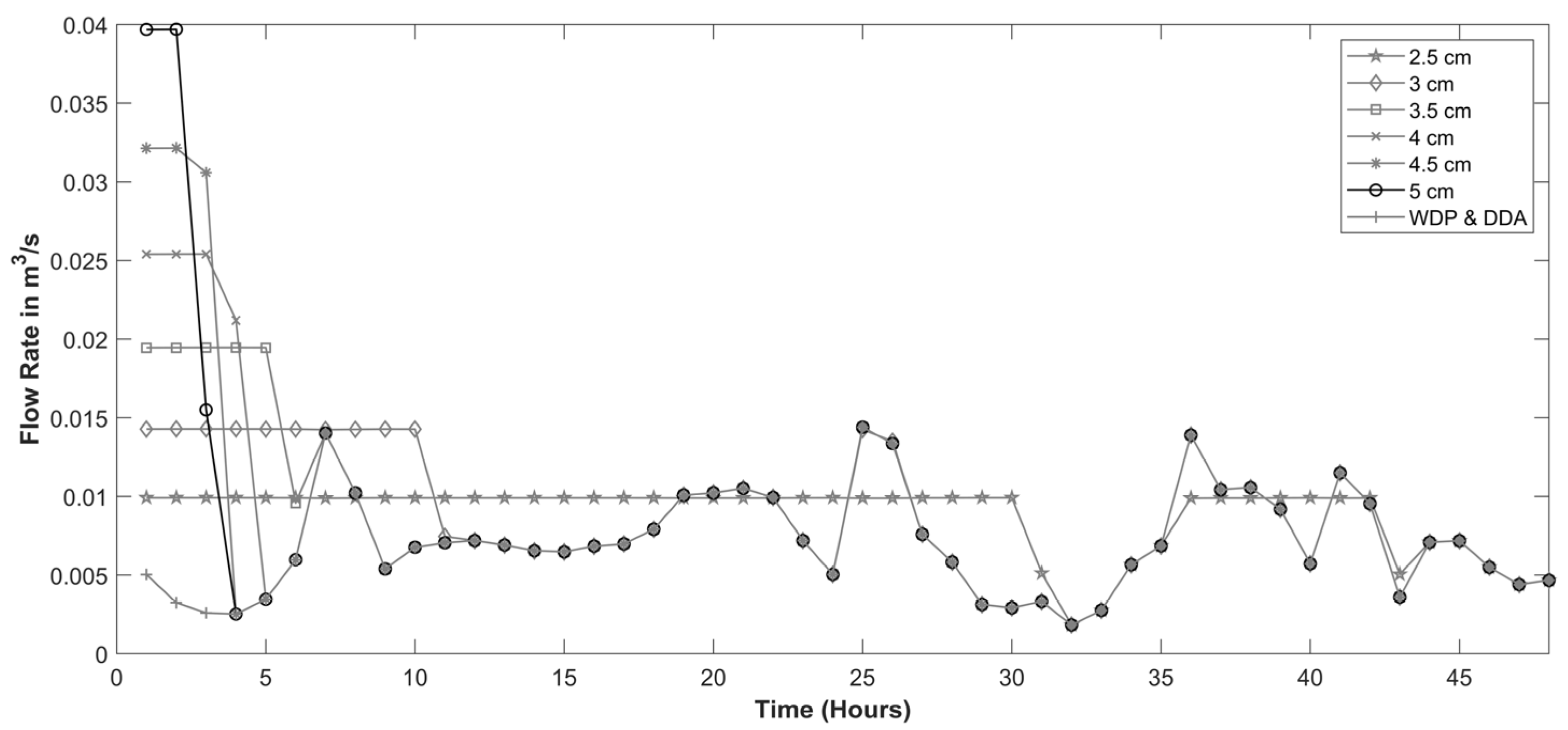
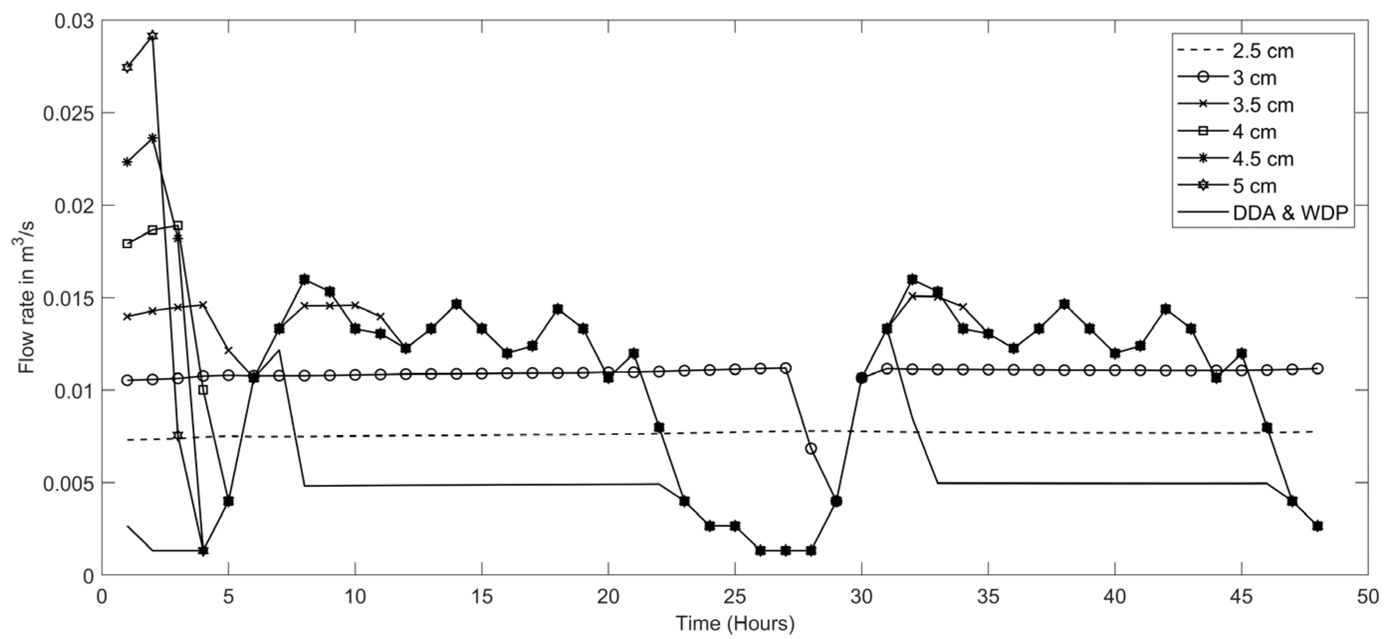
2.4. Modelling Flow to the Orifices of Private Tanks

The hydraulic model [29] used to simulate private storage tanks with a pressure-dependent demand function reflects tank filling and emptying based on orifice diameter, which changes depending on the tank’s stored volume. When the orifice operates in a binary ON/OFF mode (either fully open or closed), the coefficient C(t) remains constant during the time step ΔT, provided the maximum tank volume V_i^max is not exceeded. This allows the mass balance to be expressed as follows [29]:

$$V\left(t+\Delta T\right)=d^{fill}\Delta T-d^{act}\Delta T+V\left(t\right)\mathrm{with} d^{fill}\left(t\right)=C^{max}\sqrt{P\left(t\right)-\Delta z^{orif}}$$

(3)

where ${\mathrm{d}}^{\mathrm{f}\mathrm{i}\mathrm{l}\mathrm{l}} \left(\mathrm{t}\right)$, in cubic meter per second, is the average filling rate during ΔT; P(t), in meters, is the pressure head at time t; $\Delta {\mathrm{z}}^{\mathrm{o}\mathrm{r}\mathrm{i}\mathrm{f}}$, in meters, is the elevation of the orifice inlet; and ${\mathrm{C}}^{\mathrm{m}\mathrm{a}\mathrm{x}}$ is the maximum outflow coefficient of the orifice, which accounts for the orifice diameter via:

$$C^{max}={\displaystyle \frac{C_D\pi d^2\sqrt{2g}}{4}}$$

(4)

In Equation (4), C_D is the discharge coefficient, d is the orifice diameter, and g denotes gravitational acceleration.

The tank filling rate d_i^fill (t) and the actual customer demand d_i^act(t) at node i are defined as follows [29]:

$${d_i}^{fill}\left(P_i\left(t\right),V_i\left(t\right)\right)=\left\{\begin{array}{cc}{d_i}^{act}\left(t\right)+{\displaystyle \frac{{V_i}^{max}-V_i\left(t\right)}{\Delta T}}& V_i\left(t+\Delta T\right)>{V_i}^{max}\\ {C_i}^{max}\sqrt{P{\left(t\right)}_i-\Delta z^{orif}}& V_i\left(t+\Delta T\right)\le {V_i}^{max}\end{array}\right.$$

(5)

$${d_i}^{act}\left(P_i\left(t\right),V_i\left(t\right)\right)=\left\{\begin{array}{cc}{d}_i^{req,hum}\left(t\right)& V_i\left(t+\Delta T\right)>{V_i}^{max}\\ {C_i}^{max}\sqrt{P_i\left(t\right)-\Delta z^{orif}}+{\displaystyle \frac{V_i\left(t\right)}{\Delta T}}& V_i\left(t+\Delta T\right)\le {V_i}^{max}\end{array}\right.$$

(6)

If the tank becomes empty within ΔT, then V(t + $∆$T) = 0, and:

$${d_i}^{act}\left(t\right)={C_i}^{max}\sqrt{P_i\left(t\right)-\Delta z^{orif}}+{\displaystyle \frac{V_i\left(t\right)}{\Delta T}}$$

(7)

This implies the tank completely empties, and although the orifice is fully open, the incoming flow is insufficient to meet consumer demand.

Conversely, when the tank becomes full during ΔT, i.e., V_i(t + $∆$T) = V_i^max, the inflow is assumed constant:

$${C_i}^{max}\sqrt{P_i\left(t\right)-\Delta z^{orif}}\ge {d_i}^{act}\left(t\right)+{\displaystyle \frac{{V_i}^{max}-V_i\left(t\right)}{\Delta T}}\Rightarrow {d_i}^{fill}\left(t\right)={d_i}^{act}\left(t\right)+{\displaystyle \frac{{V_i}^{max}-V_i\left(t\right)}{\Delta T}}$$

(8)

In this case, consumer demand is fully met, so d_i^act(t) = d_i^req,hum(t), where d_i^req,hum(t) is the expected demand from the demand profile at time t.

2.5. Water Quality Model

Most water quality models investigate numerous parameters such as disinfectant residual, water color, dissolved oxygen, smell, and turbidity. As such, chlorine residuals are the most commonly investigated parameter in these parameters.

The purpose of chlorine residuals is to ensure that any disinfectant formed is safely removed by reacting with chlorine particles. This ensures that the water quality remains high. The algorithms simulating chlorine decay within a WDN are classified as steady-state or dynamic approaches to mimic this process. Particularly, the dynamic approach is more accurate as it allows the spatial distribution of pollutants to change during the simulation steps under a time-dependent demand or water demand profile (WDP). These dynamic models can be classified into Eulerian and Lagrangian-based models [23]. The pipes are usually divided into equivalent segments in the former model and into variable segments in the latter.

Therefore, based on 1-D advection-diffusion, the chlorine residual models are quantified based on Equation (9) as follows:

$${\displaystyle \frac{d{C}_{k,t}}{dt}}+v_k{\displaystyle \frac{d{C}_{k,t}}{dx}}+D_x{\displaystyle \frac{d^2{C}_{k,t}}{d{x}^2}}+R\left(C_{k,t}\right)=0$$

(9)

where ${\mathrm{C}}_{\mathrm{i},\mathrm{t}}$ is the cross-sectional average chlorine concentration (mg/L) in pipe k as a function of both time t (s) and distance x (m); ${\mathrm{v}}_{\mathrm{k}}$ represents the velocity (m/s) in pipe k; ${\mathrm{D}}_{\mathrm{x}}$ is the diffusion coefficient (m²/s) in the direction of the flow x; and $\mathrm{R}\left({\mathrm{C}}_{\mathrm{k},\mathrm{t}}\right)$ is the reaction rate (s⁻¹) measured as a function of concentration.

The reaction rate also accounts for the total source-sink function and the bulk and wall reaction intensity between chlorine and other substances in the pipes. Therefore, the chlorine reaction rate can be further categorized using the first-order reaction in Equation (10) [23].

$$R\left(C_{k,t}\right)=-k_0{C}_{k,t}$$

(10)

where ${\mathrm{k}}_0$ is the first-order reaction rate (s⁻¹), the chlorine decay rate would be proportional to the chlorine concentration to the first power if ${\mathrm{k}}_0$ is the first-order reaction rate (mg·s/L), represented in Equation (11) as follows:

$$k_0=k_b+{\displaystyle \frac{k_w{k}_f}{r_h(k_w+k_f)}}$$

(11)

where ${\mathrm{k}}_{\mathrm{b}}$ is the coefficient of bulk decay (s⁻¹), ${\mathrm{k}}_{\mathrm{w}}$ is the coefficient of wall demand (m/t), ${\mathrm{r}}_{\mathrm{h}}$ is the hydraulic radius (m), and ${\mathrm{k}}_{\mathrm{f}}$ is the coefficient of mass transfer (m/s). Each of these factors needs to be taken by field calibration. However, they can be assumed based on the experience of an engineer [23,32]. Furthermore, there are other factors including pH level and temperature, that can impact the concentration of chlorine. However, they are assumed to remain consistent in the simulation to ensure a fair test when analyzing the different parameters of the private tank. Thus, the assumed pH value based on the characteristics of the network in Dubai was taken as 7.6, and the temperature of water was assumed to $22 °\mathrm{C}$ [30]. Such models are incorporated into the simulation software to predict the chlorine residual in WDNs by considering their reaction with pipe walls and transportation.

Mathematical models incorporating chlorine kinetics, reaction rates, and transport phenomena are viable for simulating water chlorination. Water treatment systems can utilize models to forecast chlorine concentrations and disinfection outcomes. These models are established and authenticated through the application of actual data. The outcomes of the simulation aid in improving the chlorination process by enhancing the effectiveness of disinfection and reducing the production of disinfection by-products. The process of simulating water chlorination is commonly executed through the use of specialized software and tools. This enables water treatment experts to make informed decisions and ensure the provision of potable water that meets safety standards [25,32,33].

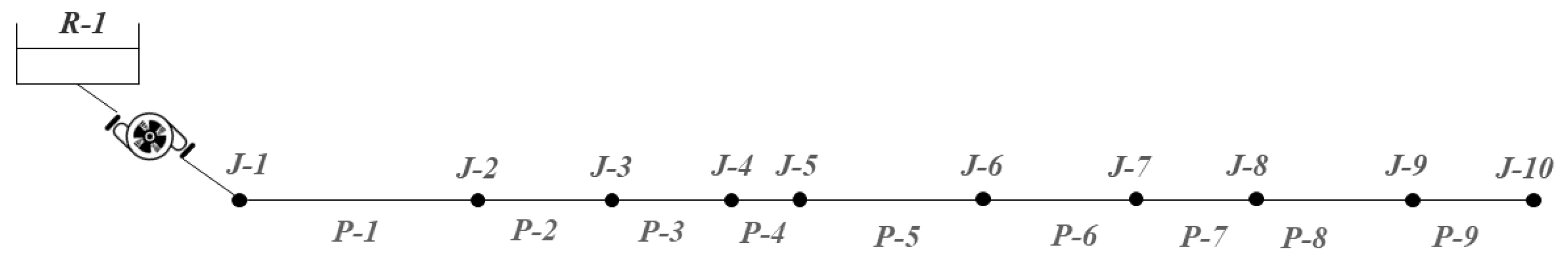
2.6. Sample Networks

The first sample WDN contains a single node connected directly to a reservoir by a single pump, as shown in Figure 2. The purpose of examining such a small network is to show the impact on different parameters of the network, such as pressure, flow, pump scheduling, aging, and chlorine concentration.

The second sample WDN contains a single source that supplies water using a single pump to a series of ten consecutive junctions, as shown in Figure 3. The purpose of examining this network configuration is to account for the head loss on the receiving parameters of the WDN. Furthermore, using this network allows us to see the downstream impacts due to the changes in the characteristics of the private tank’s parameters at the upstream junction.

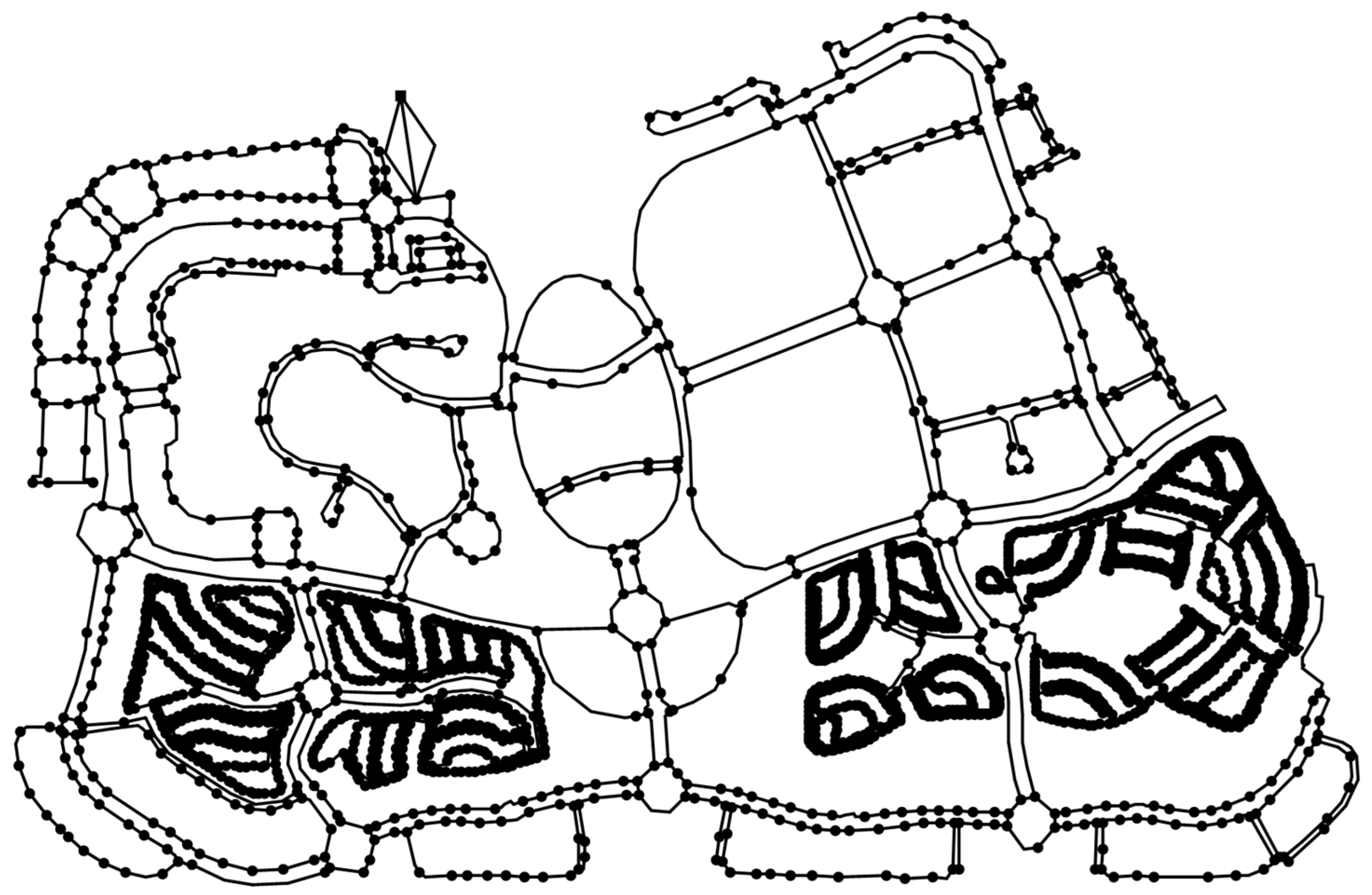
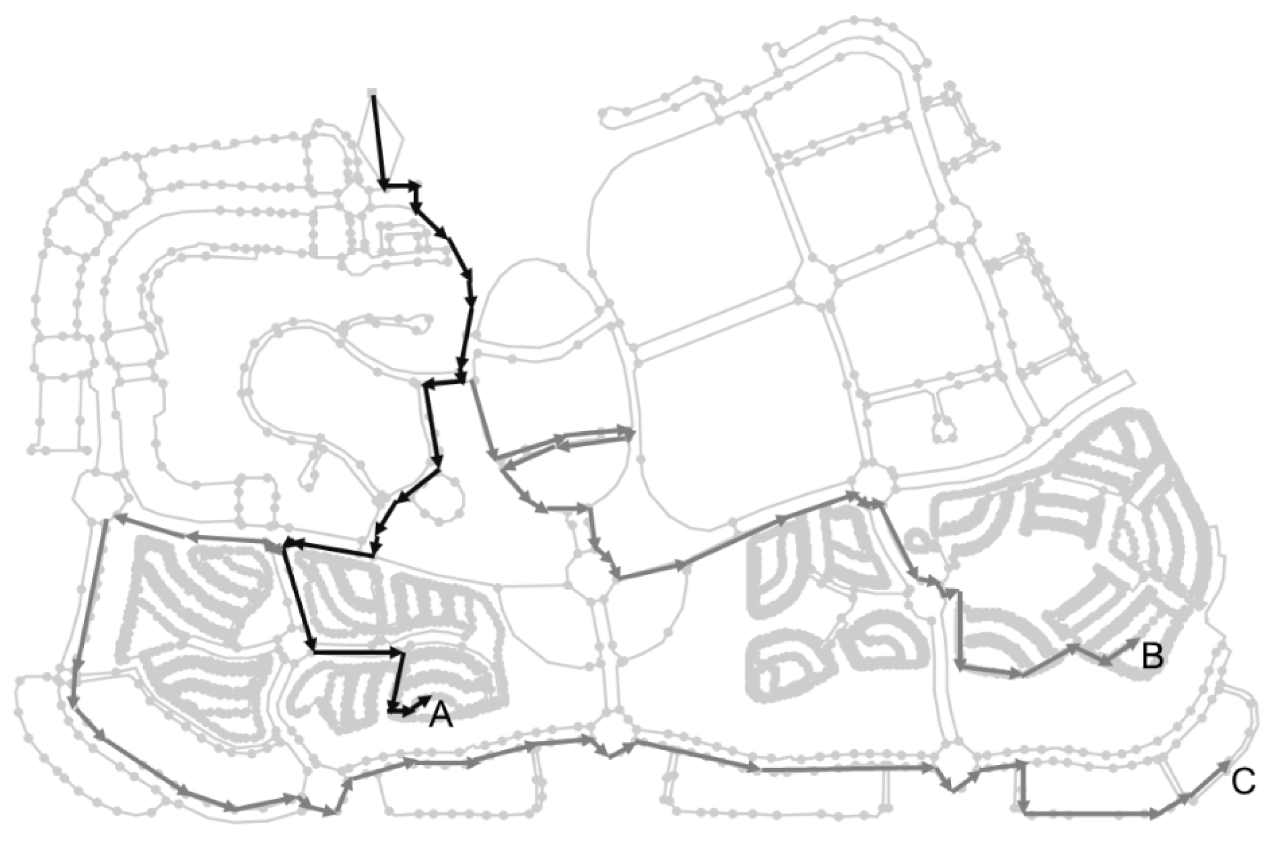
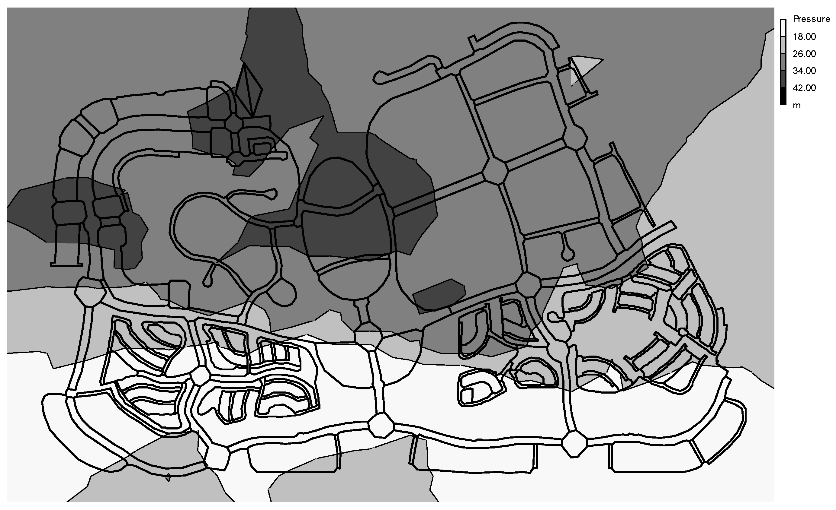
2.7. Real-World Network

The Dubai Silicon Oasis (DSO) network is typically a branched network comprising 2550 junctions and 2750 pipe links, see Figure 4 [31]. Water is sourced from a singular reservoir and is distributed through three parallel pumps. The range of pipe diameters falls within the range of 150 mm to 900 mm, whereas the daily per capita demand is approximately 300 liters per day [30]. The projected user count is approximately 165,000 individuals. The region’s topography exhibits altitude fluctuations, with limited regions surpassing the 30-m elevation of the reservoir’s apex. The network’s nodal characteristics exhibit variability due to the diverse structures present within the area, including residential buildings, villas, commercial buildings, educational institutions, governmental offices, and medical facilities. As such, the water quality analysis would use this network to test the reliability when integrated with private tanks.

2.8. Calibration Process

The calibration process in this study was tailored to its specific purpose: hydraulic and water quality modelling, since calibrated models are not universally applicable. Calibration involved reconstructing network geometry and estimating key parameters using often incomplete or erroneous data, necessitating field verification, which is limited by DEWA regulations. Integrating Geographic Information System (GIS) data helped identify missing information by comparing pipe layouts with road networks. While most physical parameters like pipe diameters and pump characteristics were stable, pipe roughness required calibration through flow rate comparisons in the literature due to its variability with age.

Water demand data, sourced from well-maintained DEWA meters, did not require calibration, but tank sizes were verified against developer-provided data. For the chlorine concentration models, wall decay coefficients were calibrated using the literature and lab data, although the high-quality desalinated water in Dubai reduced the need for changes. The calibration process also included aligning model pipes with GIS topography and verifying tank sizes at 12 locations per network. Variations were minor (under 4 percent), largely due to differences in building types and layouts. An error analysis was conducted to quantify uncertainties in tank sizes, pipe roughness, and chlorine concentrations using statistical measures like standard deviation. A summary of the calibration process is provided in Figure 5.

2.9. Procedure of the Application

The approach for adopting this technique is based on the EPS of the first-order kinetic equation and chlorine decay for a network with integrated private tanks using PDA in WQnetXL [25]. Furthermore, to validate the findings from WQnetXL, EPANET analysis was used to determine the chlorine concentration at the junctions. Like water age analysis, the inflow curve obtained from different orifice sizes and retention times was plugged into the EPANET model for water quality analysis. The process adopted in both approaches is based on the Lagrangian Transport Algorithm (LTA), which utilizes Equations (9) and (11) to simulate the chlorine concentration at each part of the junction.

The same methodology has been adopted to facilitate the integration of private tanks. As for water quality models, the principle of PDA with LTA utilizes the sizing of a segment carrying discrete water units. As the simulation continues, the size of upstream nodes can increase with more water entering the pipe, while having an equal loss in the size of the downstream segment when water leaves the pipe. However, the overall volume of every pipe segment would not change; therefore, the segments’ size of the leading and trailing segments would also remain unchanged. For the LTA model to perform quality analysis, the following actions were performed at each time step:

• The value for chlorine concentration was updated to reflect any reaction that has occurred over the time interval.
• For each upstream junction, the water from the leading segments of the pipe with the flow was mixed to calculate the new value of chlorine concentration. The volume contributed from each segment would equal the product of the pipe flow and the time interval. With the upcoming flow, if the volume exceeded that of the segment, then the segment was removed, and the next one behind it started contributing to the volume.
• The new quality was calculated for every junction based on the total inflow mass divided by the total inflow volume.
• The concentration at the junction was changed based on the contribution of external water quality sources, such as networks with two reservoirs.
• Finally, a new segment was built in the pipes, and the flow came out of the node. The volume of this new segment was again calculated using the product of the flow rate and time interval. Its quality was equated to the new quality found for the junction.

In this algorithm, the number of segments was limited for quicker analysis; new segments were only produced if the new junction’s quality differed more than a user-specified tolerance from the quality of the previous segment. This process was repeated for each time step.

2.10. Simulation

For this simulation, the first step was to compare the performance of DDA models with that of integrated private tanks. The next step was to increase the orifice diameter and retention time to observe their impact on the concentration of chlorine. As such, any external factor, including pipe wall reaction and bulk decay rate, was not considered, since the main emphasis was on observing private tank integration’s impact on simple networks. The initial quality of the reservoir was kept at 3 mg/L for each network, because this comes under the range of chlorine concentration specified by the DEWA. The simulation ran based on the following steps for 72 h during weekdays:

• Networks 1, 2, and DSO were run using DDA in EPANET, followed by the integration of private tanks using different orifice sizes and retention times under PDA.
• The water quality parameters (wall coefficient, bulk coefficient, limiting concentration and wall correlation) were selected based on this region.
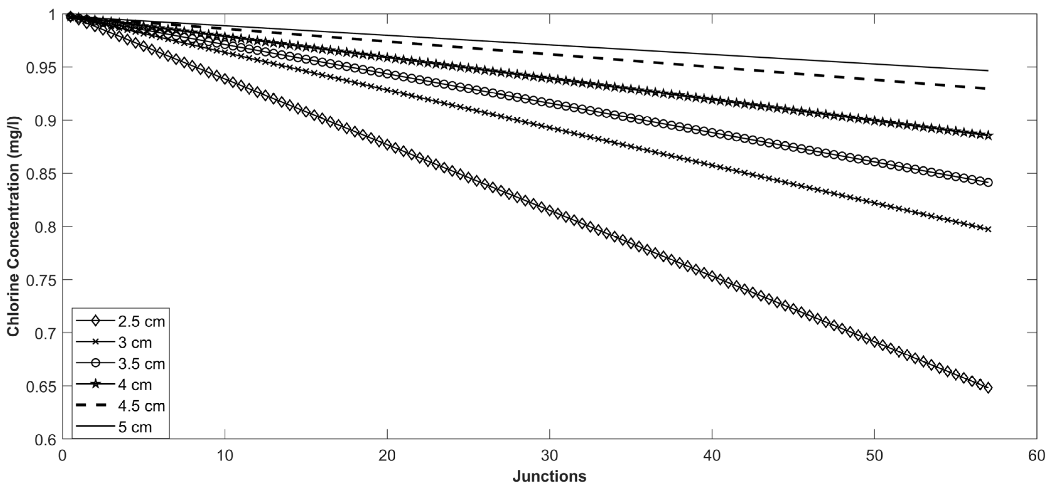
• The selected range of orifice size varied from 2 cm to 5 cm; the retention time varied from 6 h to 24 h.
• Each variation of orifice size was tested using LTA while keeping the retention time constant.
• Then, the same water quality simulation was performed by changing the retention time of the private tanks whilst keeping the orifice size the same.
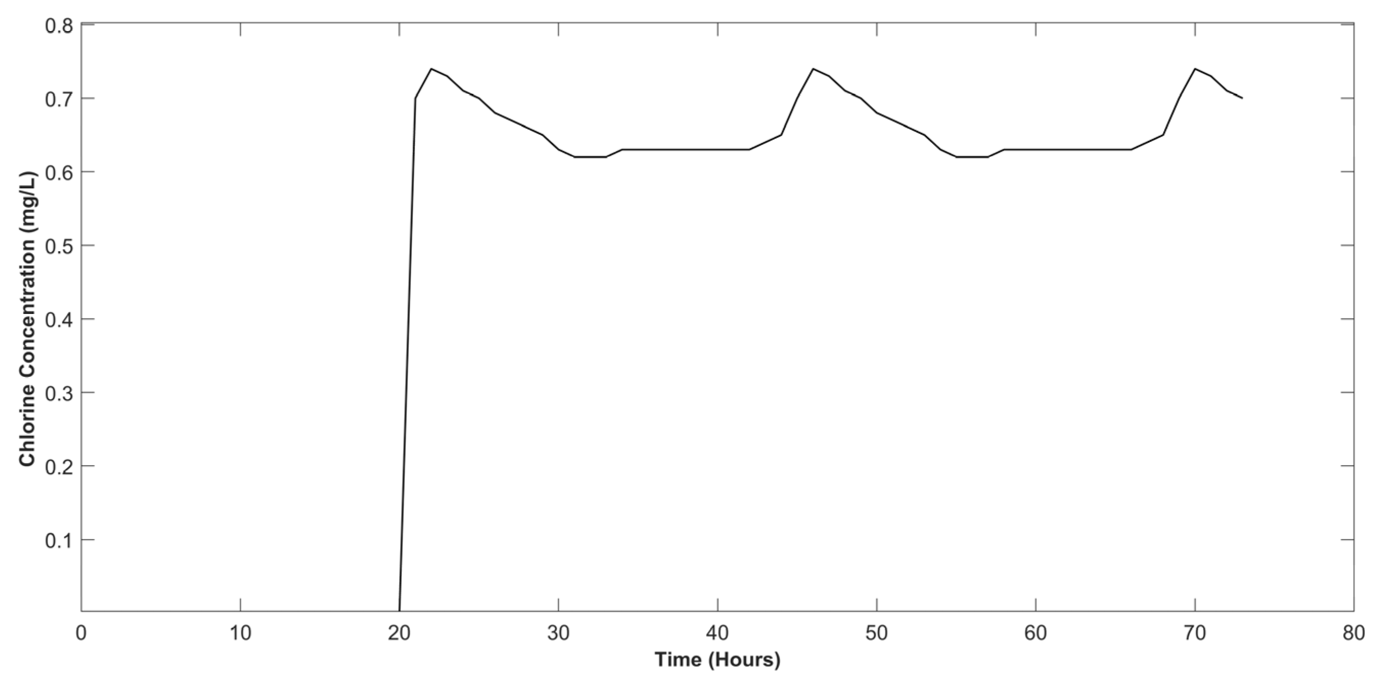
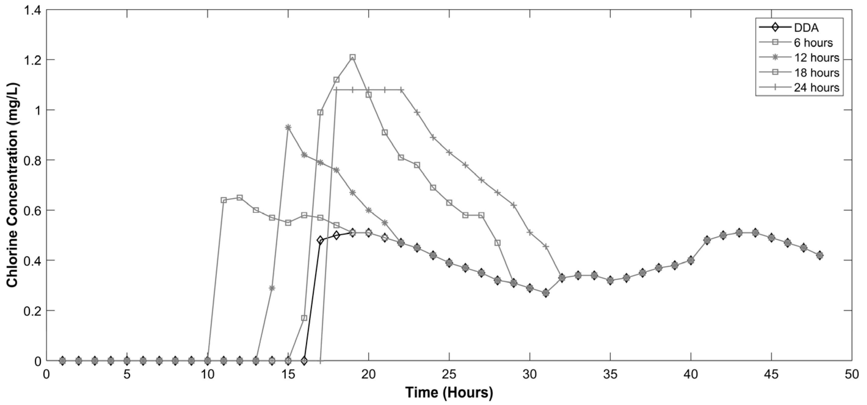
• A comparison of chlorine concentrations over time was graphed for the different scenarios.

The next part of the simulation considers the water quality reliability indicators that assess the junction’s chlorine concentration. These indicators calculate the network’s performance by using a ratio of junctions above the chlorine concentration level to the network’s overall junctions. The chlorine concentration level indicated by DEWA suggests that the chlorine concentration should always be greater than 0.3 mg/L at each junction. Therefore, a reliability assessment was carried out by changing the tank parameters of the network and comparing them with the design set up by engineers (DDA models). This reliability assessment followed the same steps mentioned previously to obtain the chlorine concentration. Afterward, the reliability indicator used Equation (12) to determine whether the junctions have passed or failed the assessment. For each retention time and orifice size, the reliability indicators in Equation (13) were used to calculate the percentage of junctions that have passed.

$$f_{t,Q}=\left\{\begin{array}{c}1, if C_{i,t}>0.3 \mathrm{mg}/\mathrm{L} \\ 0, if C_{i,t}\le 0.3 \mathrm{mg}/\mathrm{L}\end{array}\right.$$

(12)

$$R_Q=\left({\displaystyle \frac{\sum _{t=1}^N{f}_{t,Q}}{N}}\right)\%$$

(13)

where ${\mathrm{f}}_{\mathrm{t},\mathrm{Q}}$ denotes the failure event/condition at each time step t for the quality indicator (chlorine concentration) and ${\mathrm{R}}_{\mathrm{Q}}$ represents the percentage of passing and other variables.

3. Results and Discussion

For the first part of the following analysis, the comparison was graphed to establish the variation of chlorine level in the junction, with different orifice sizes and retention times.

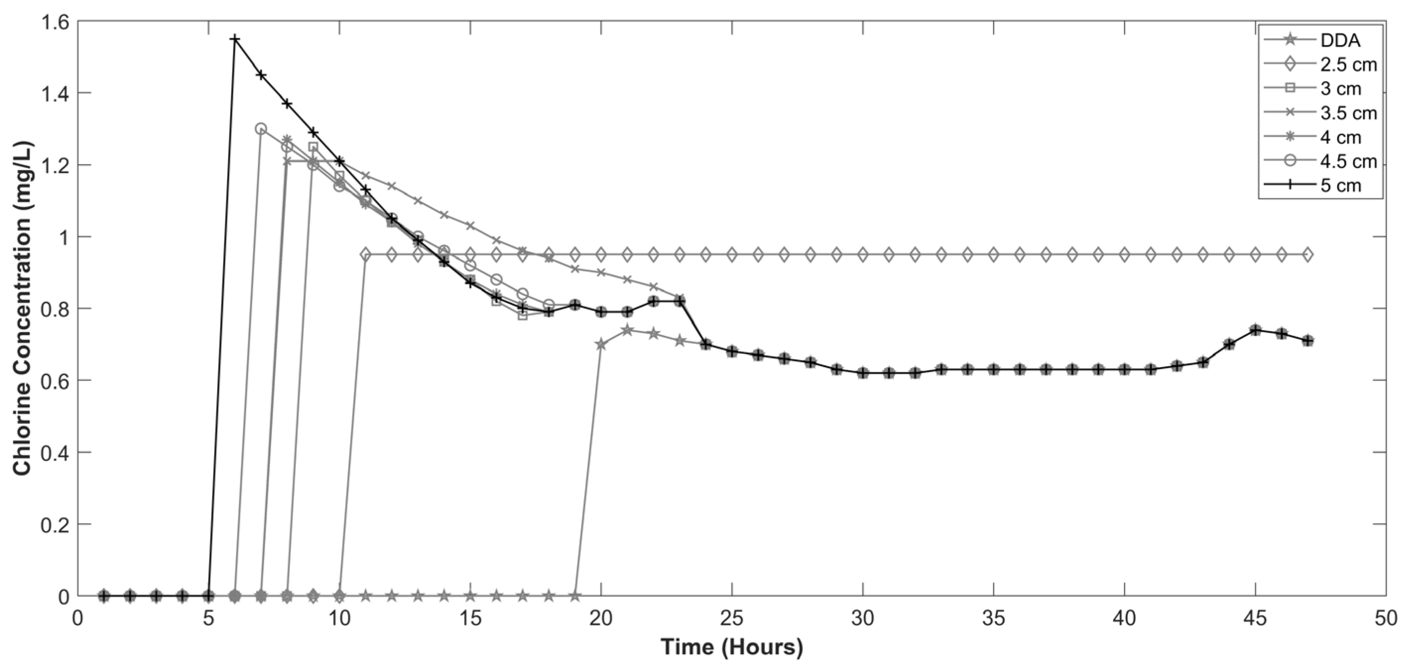
3.1. Impact of Orifice Size on Chlorine Concentration

As a result of the simulation of the DDA model of Network 1, Figure 6 shows the variation of the chlorine level through time. The demand profile is depicted in Figure 7.

It can be observed in Figure 6 that the chlorine level fluctuates continuously and periodically from 22 h to 72 h. The periods where the chlorine level drops are due to high demand in the network, which increases the flow rate, as it coincides with the high demand at 32 h in Figure 7. As a result, the chlorine level drops during the peak demand period. This impact was also validated by [34], who stated that an increased flow rate would reduce the chlorine concentration.

By comparing the DDA model to the model of integrated private tanks with different orifice sizes, Figure 8 shows the fluctuation level of chlorine at the junction for the network over the span of 48 h (a time span of 72 h was ignored because the behavior of chlorine concentration repeated). Furthermore, Figure 9 depicts how the inflow at the orifice inlet coincides with the quality level and the flow rate.

Based on the results shown in Figure 8, it can be observed that the chlorine concentration reaches a maximum level for the highest orifice inlet since it has the highest flow. As such, the chlorine concentration reaches the maximum value of 1.6 mg/L at a time of 6 h, compared to other inlet sizes that take another hour or more to reach the maximum value. Secondly, as soon as the tank is filled, the flow behavior is similar to DDA in each case of orifice size from 3 cm to 5 cm. Afterward, the chlorine concentration decreases based on the flow rate. Since this happens very quickly, the chlorine concentration drops immediately because the flow rate becomes very similar to that of DDA. However, based on observation after 12 h, it can be noted that the orifice size of 2.5 cm was not completely filled throughout the simulation; as a result, the chlorine concentration remained constant. Furthermore, the chlorine concentration of the orifice inlet of 2.5 cm remained higher than DDA and other cases after the time step of 15 h, as the flow rate for the orifice inlet of 2.5 cm remained higher than any of the other cases (because the volume of the private tank did not reach maximum capacity). This indicates that larger orifice sizes can increase the chlorine concentration because they are able to reach the junction quickly without reacting to the boundary wall. As a result, increasing the orifice size results in an increase in the chlorine levels at the junction.

Similar results were observed for Network 2, which can be seen in Figure 10, which compares different orifice inlets with the DDA model for junction 8.

This network also validates that increasing the orifice size would increase the chlorine level due to the high flow rate until the water level in the tank does not reach its full capacity. However, higher orifice sizes fill up the tank quickly, decreasing the system’s flow rate and ultimately decreasing the concentration. For instance, in Figure 11, the chlorine level has dropped from 1.7 mg/L to 0.6 mg/L in a time span of 9 h for the orifice inlet of 5 cm. This decrease in chlorine level is the highest when compared to another orifice inlet, since the flow decreases rapidly when the orifice inlet closes. This is evident from Figure 11, which showcases the drastic change in flow when the orifice size is decreased from 2 cm to 5 cm. The higher corresponding flow for orifice sizes of 5 cm resulted in higher chlorine concentration in the pipe in Figure 10. As a result, this can impact the chlorine concentration level in the network when the network has a much lower demand. Hence, lower orifice sizes are again preferred since they retain higher chlorine concentration for a long period of time, since the tank does not reach its maximum capacity.

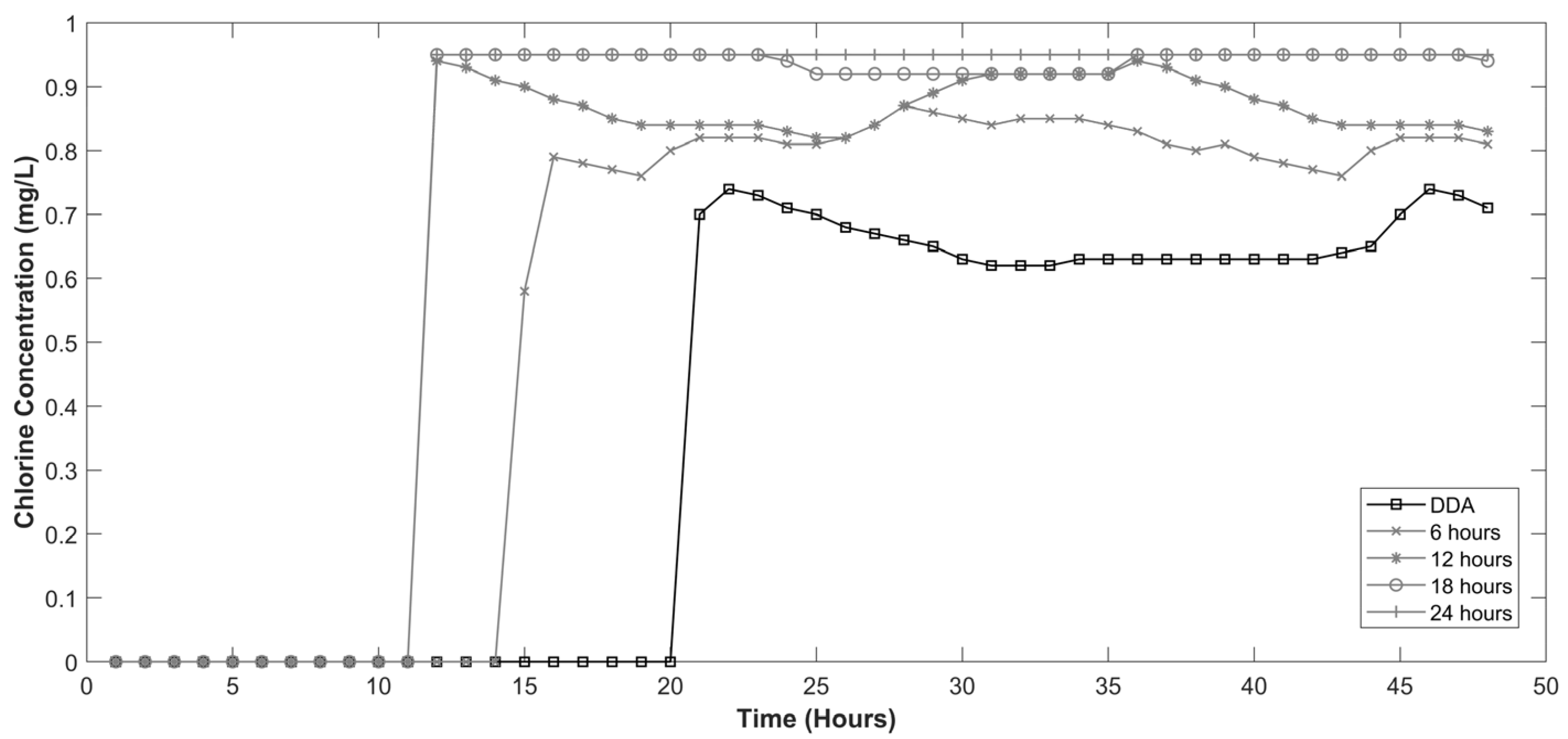
3.2. Impact of Retention Time on Chlorine Concentration

The impact of retention time relatively affects flow based on the water level in the tank, which can ultimately open or close the orifice. Under optimal orifice settings, the behavior of filling and emptying is regularly encouraged, which remains the same regardless of the tank’s retention time change. As a result, the only notable impact of changing retention time is observed when the orifice is sufficient to satisfy demand and discourage any drop in the water level. Such a scenario is observed when a float valve is placed in tanks that control the opening and closing of the orifice based on the water level. As such, the orifice sizes are kept larger to encourage quick opening and closing when water drops below a certain set level.

Therefore, for Network 1, the orifice level was kept at a constant value of 2.5 cm, while the retention time was changed to observe the impact on chlorine concentration. As a result, Figure 12 shows the chlorine level for the junction over time for the DDA and integrated tank models with different retention times.

From Figure 12, it can be observed that increasing the retention times of the private tank causes the chlorine concentration in junctions to increase. This is because the time the orifice inlet remains open increases, which causes more flow to enter the system. As expected from Figure 12, the private tank retention time of 6 h tends to fill first, followed by 12 h, then 18 h and 24-h retention time, which causes the chlorine concentration to increase over time. As soon as the private tank is full, the graph of chlorine concentration starts to become similar to that of the DDA model. As a result, the lower retention time of 6 h has behavior similar to that of the DDA model. It is also important to note that the maximum difference between the peak chlorine level of the DDA model and the model with a retention size of 24 h is 0.3 mg/L. This difference validates that inserting a certain storage volume tends to impact concentration because more water is added to the system.

Another observation from Figure 12 is that the variation in chlorine concentration remains similar for all the retention sizes. The changes in the chlorine level variation only happen when the tank’s water level reaches the maximum capacity. For instance, when observing the chlorine level from Figure 12 for the retention times of 18 h and 24 h, it can be observed that the variation of chlorine concentration remained similar since the tanks for both retention times did not reach the maximum capacity. There is a slight variation at 24 h, where the tank size with a retention time of 18 h reaches maximum capacity, which shows a small drop in chlorine concentration of 0.02 mg/L. Before this time, both curves were similar due to the longer opening of the orifice.

For Network 2, the same simulation was carried out to produce the chlorine concentration level for each junction. As such, the downstream junction (J-8) results are presented in Figure 13, which shows the chlorine level pattern for the DDA model and integrated private tanks with different retention times.

The results from Figure 13 validate the findings observed in the Network 1 simulation, as the chlorine levels tend to increase with increasing retention times. The model shows a relatively large difference in concentration levels because more junctions are present in the network, allowing more flow to be added. The maximum difference between the smallest retention time of 6 h and the largest 24 h retention time was close to 0.4 mg/L. Another observation based on Figure 13 shows that the chlorine concentration takes more time to increase for higher retention times. This is due to more flow being utilized by upstream nodes.

3.3. Reliability Analysis for the Real-Time Network

As observed for the cases of Network 1 and Network 2, the impact of both orifice sizes and retention time of the private tank tends to impact the chlorine concentration level due to the changes in flow. Therefore, a reliability analysis of the DSO network was conducted to account for whether these changes in chlorine concentration result in any failure when the network is set up without integrating private tanks (as done in the design stage). The analysis results presented in

Table 1. Percentage of junctions that passed the assessment based on different orifice sizes and retention times for the DSO network.

Retention Time	Orifice Sizes
	2.5 cm	3 cm	3.5 cm	4 cm	4.5 cm	5 cm
6 h	91%	92%	92%	94%	94%	95%
12 h	94%	95%	95%	96%	96%	97%
18 h	97%	98%	98%	98%	98%	98%
24 h	98%	99%	99%	100%	100%	100%

show the network’s performance with different orifice inlet sizes and retention times.

It can be observed from Table 1 that increasing the orifice inlet increases the network’s reliability because the system’s flow rate increases. Even when keeping an optimal orifice size of 2.5, the percentage of the junction with chlorine level higher than the standard level by DEWA is close to 98% for a retention time of 24 h. For an orifice size that goes up to 5 cm (retention time of 24 h), the optimal percentage of junction that had passed in the entire simulation was 100%, because larger orifice sizes cause a higher flow rate, resulting in increased chlorine concentration. Failure in the system largely occurs due to smaller retention times, which indicates a change in the initial concentration of the chlorine level, since the network would not be able to satisfy the demand quality for the consumer. As such, the initial chlorine dosage had to be increased by 50% for the smallest orifice size and retention time to achieve full network reliability without any failure.

In Table 1, it can also be observed that increasing the retention time increases the network’s reliability more effectively than changing orifice sizes. The percentage of passing increases from 94% to 100% when changing the retention time from 6 h to 24 h for an orifice size of 4 cm. As validated before from the simple networks, this is due to the system’s increased flow, which increases the chlorine concentration level. Moreover, most of these failures only occur in the simulation’s beginning time step, after which they become more similar. Furthermore, it implies again that the initial chlorine dosage in the reservoir has to increase to satisfy the water quality parameters.

Finally, the results of chlorine concentrations for different orifice sizes in the DSO network are showcased using flow path C shown in Figure 14. The pressure distribution of the network is depicted in Figure 15.

Based on the selected flow path C, the chlorine concentration obtained along the junctions from the reservoir to Junction C for different orifice sizes is presented in Figure 16.

From Figure 16, it can be noted that increasing the orifice size results in an increase in the chlorine concentration due to high flow. As such, the observed chlorine concentration for the last junction is closer to 0.97 mg/L for the orifice size of 5 cm. In comparison to the smallest orifice size, the chlorine concentration has decreased by 30% during the filling period of private tanks. However, this impact is only observed during the filling time of the tank; thereafter, once the tank has reached its full capacity, the observed concentration gradually decreases. Moreover, as the water flows through the pipe, the chlorine concentration decreases in the junction due to lower pressure, as seen in Figure 15, which decreases the overall flow of the pipe.

At the end of the analysis, it is also worth pointing out the limitations of the network; the uncertainty of WDP remains a factor due to the integration of private tanks. Secondly, the analysis assumes that the flow rate at each time step remains constant. While this assumption is quite helpful for quick analysis, it dampens some of the peaks that can be observed during a relative time step. As such, it increases the uncertainty of the reliability indicators as it does not account for any changes in demand during the time step. Finally, due to the restriction in accessing real-time networks, the coefficients were based on the literature rather than actual field tests for the DSO model. Data from a field test could have improved the accuracy of the result; however, since each condition had an equal fair test, it would not have impacted the findings.

From the results, it was noticed that larger orifice sizes were initially able to provide high chlorine concentration throughout the network, but were not able to maintain it since the tank became full and the flow in the system dropped. Ideally, the best case observed in this study suggested controlling the orifice area based on the pressure-demand relation [29]. This would allow continuous flow within the system without the water parcel being halted, thereby improving the water quality in the system.

Similarly, when the tank is being filled, the chlorine concentration would remain quite high for larger tank sizes compared to smaller tank sizes. In fact, the concentration of chlorine was 12% higher for large tanks (24 h retention time) when compared with the smallest tank size with a retention time of 6 h. The presence of more chlorine allows the water quality to be maintained as it reacts with any contaminants to achieve the standard required of drinking water. Similarly, the reliability with tank parameters was quite high, as large orifice sizes and retention times were able to achieve the highest reliability. In terms of scale, a study by Garcia-Avila et al. [26] mentions that 45% of the junctions were below index if they had unaccounted design constraints. The failure percentage for this analysis was significantly lower than the addition of private tanks on the system, and higher pipe diameters are advised in the Code of Practice [30].

3.4. Error Analysis

As observed during the investigation of water age, the impact of WDP is limited. Thus, when extended towards water quality, similar observations were made. However, in the chlorine concentration parameter, another key parameter is the wall reaction coefficient factor, which directly impacts the chlorine concentration. Since there was a limitation during the calibration of the wall decay coefficient parameters, due to restrictions on accessing the network, the range of values that was considered can be found in the Code of Practice [30]. The impact of different decay values (0.5 to 1) was implemented in the model to see the changes in the chlorine concentration.

Table 2. Change in chlorine concentration of the networks at peak hour for the DDA model due to different values of decay coefficient.

		Sample Network		Real-World Network
		1	2	DSO
Chlorine Concentration (mg/L)	Maximum Change	0.12	0.24	0.54
	Average Change	0.12	0.15	0.29
	SD	0	0.45	0.87

shows the differences in the value of chlorine concentration when using different values of the wall decay coefficient.

Based on the Code of Practice, the range of wall coefficient lies between 0.5 to 1, which shows the percentage uncertainty of chlorine concentration to range from 7% to 11% from the result in Table 2 throughout the difference junction for each network. These changes go higher in areas with lower flow rates, where maximum change in concentration was observed at 0.54 mg/L. While these differences are acceptable, such differences in values can increase or decrease the actual concentration of chlorine when applied in a real-life network. However, the maximum absolute uncertainty of chlorine concentration of 0.54 mg/L was concerning. However, in real life, the network can be regulated by performing calibration by doing laboratory testing for chlorine. Therefore, these errors can be accepted and are consistent for different orifice sizes and retention times, which does not impact the overall investigation of the result.

4. Conclusions

This study demonstrates the critical role of private storage tank parameters, namely, orifice size and retention time, in influencing chlorine concentration and network reliability in water distribution systems. Simulation results revealed that larger orifice sizes, such as 5 cm, led to higher initial chlorine concentrations, reaching peak values of up to 1.6 mg/L within 6 h. However, once the tank reached capacity, the flow rate dropped sharply, causing the chlorine concentration to decrease to as low as 0.6 mg/L over the next 9 h. In contrast, smaller orifice sizes, particularly 2.5 cm, maintained more stable concentrations throughout the simulation, as the tank did not fill completely and thus sustained a higher flow rate over time.

Retention time also played a significant role in water quality performance. Increasing retention time from 6 to 24 h improved chlorine concentration, with differences as high as 0.3 to 0.4 mg/L between the shortest and longest durations. Moreover, network reliability improved with both larger orifice sizes and longer retention times. For instance, the percentage of junctions meeting quality standards rose from 91 percent to 100 percent when the orifice size increased from 2.5 cm to 5 cm and retention time increased from 6 to 24 h.

These findings emphasize the need to account for tank-specific parameters in network design and quality analysis. Future work should consider integrating real-time smart meter data to improve the accuracy and efficiency of demand profiling. Additionally, collecting data on pipe wall decay from actual networks would improve the precision of chlorine decay modeling.

References

1. García-Ávila, F.; Avilés-Añazco, A.; Ordoñez-Jara, J.; Guanuchi-Quezada, C.; Flores del Pino, L.; Ramos-Fernández, L. Modeling of residual chlorine in a drinking water network in times of pandemic of the SARS-CoV-2 (COVID-19). Sustain. Environ. Res. 2021, 31, 12. [Google Scholar] [CrossRef]
2. Boulos, P.F.; Altman, T.; Jarrige, P.A.; Collevati, F. Discrete simulation approach for network-water-quality models. J. Water Resour. Plan. Manag. 1995, 121, 49–60. [Google Scholar] [CrossRef]
3. Mau, R.E.; Boulos, P.F.; Bowcock, R.W. Modelling distribution storage water quality: An analytical approach. Appl. Math. Model. 1996, 20, 329–338. [Google Scholar] [CrossRef]
4. Hallam, N.B.; West, J.R.; Forster, C.F.; Powell, J.C.; Spencer, I. The decay of chlorine associated with the pipe wall in water distribution systems. Water Res. 2002, 36, 3479–3488. [Google Scholar] [CrossRef]
5. Chhipi-Shrestha, G.; Mohammadiun, S.; Ishaq, S.; Hu, G.; Mian, H.; Pokhrel, S.; Hewage, K.; Sadiq, R. Modeling hydraulics and water quality in distribution networks: A review of existing mathematical techniques and software. In Water Engineering Modeling and Mathematic Tools; Elsevier: Amsterdam, The Netherlands, 2021; pp. 187–212. [Google Scholar]
6. Chun, D.G.; Selznick, H.L. Computer modeling of distribution system water quality. In Computer Applications in Water Resources; ASCE: Reston, VA, USA, 1985; pp. 448–456. [Google Scholar]
7. Males, R.M.; Grayman, W.M.; Clark, R.M. Modeling water quality in distribution systems. J. Water Resour. Plan. Manag. 1988, 114, 197–209. [Google Scholar] [CrossRef]
8. Murphy, S.B. Modeling Chlorine Concentrations in Municipal Water Systems. Doctoral Dissertation, College of Engineering, Montana State University-Bozeman, Bozeman, MT, USA, 1985. [Google Scholar]
9. Shah, M.; Sinai, G. Steady state model for dilution in water networks. J. Hydraul. Eng. 1988, 114, 192–206. [Google Scholar] [CrossRef]
10. Wood, D.J.; Ormsbee, L.E. Supply identification for water distribution systems. J.-Am. Water Work. Assoc. 1989, 81, 74–80. [Google Scholar] [CrossRef]
11. Fowler, A.G.; Jones, P. Simulation of water quality in water distribution systems. In Proceedings of the Water Quality Modeling in Distribution Systems 1991, Cincinnati, OH, USA, 4–5 February 1991; pp. 4–5. [Google Scholar]
12. Rossman, L.; Boulos, P.; Altman, T. Discrete Volume-Element Method for Network Water-Quality Models. J. Water Resour. Plan. Manag. 1993, 119, 505–517. [Google Scholar] [CrossRef]
13. Clark, R.M.; Grayman, W.M.; Males, R.M.; Hess, A.F. Modeling contaminant propagation in drinking-water distribution systems. J. Environ. Eng. 1993, 119, 349–364. [Google Scholar] [CrossRef]
14. Liou, C.P.; Kroon, J.R. Modeling the propagation of waterborne substances in distribution networks. J.-Am. Water Work. Assoc. 1987, 79, 54–58. [Google Scholar] [CrossRef]
15. Grayman, W.M.; Clark, R.M.; Males, R.M. Modeling distribution-system water quality; dynamic approach. J. Water Resour. Plan. Manag. 1988, 114, 295–312. [Google Scholar] [CrossRef]
16. Tansley, N.S.; Brammer, L.F. Chlorine residual modelling in distribution: The improvement of taste and the maintenance of effective disinfection. In Integrated Computer Applications in Water Supply (Vol. 2) Applications and Implementations for Systems Operation and Management; John Wiley and Sons Ltd.: West Sussex, UK, 1994; pp. 111–126. [Google Scholar]
17. Kiéné, L.; Lu, W.; Lévi, Y. Relative importance of the phenomena responsible for chlorine decay in drinking water distribution systems. Water Sci. Technol. 1998, 38, 219–227. [Google Scholar] [CrossRef]
18. Lu, W.; Kiéné, L.; Lévi, Y. Chlorine demand of biofilms in water distribution systems. Water Res. 1999, 33, 827–835. [Google Scholar] [CrossRef]
19. Ostfeld, A.; Kogan, D.; Shamir, U. Reliability simulation of water distribution systems–single and multiquality. Urban Water 2002, 4, 53–61. [Google Scholar] [CrossRef]
20. Gupta, R.; Dhapade, S.; Ganguly, S.; Bhave, P.R. Water quality based reliability analysis for water distribution networks. ISH J. Hydraul. Eng. 2012, 18, 80–89. [Google Scholar] [CrossRef]
21. Tryby, M.E.; Boccelli, D.L.; Uber, J.G.; Rossman, L.A. Facility location model for booster disinfection of water supply networks. J. Water Resour. Plan. Manag. 2002, 128, 322–333. [Google Scholar] [CrossRef]
22. Kang, D.; Lansey, K. Real-time optimal valve operation and booster disinfection for water quality in water distribution systems. J. Water Resour. Plan. Manag. 2010, 136, 463–473. [Google Scholar] [CrossRef]
23. Wang, Y.; Zhu, G.; Yang, Z. Analysis of water quality characteristic for water distribution systems. J. Water Reuse Desalin. 2019, 9, 152–162. [Google Scholar] [CrossRef]
24. Belcaid, A.E.; Taghlabi, F.; Tounsi, A. Chlorine Decay Modeling in a Water Distribution Network in Mohammedia City, Morocco. Ecol. Eng. Environ. Technol. (EEET) 2023, 24, 269–278. [Google Scholar] [CrossRef]
25. Giustolisi, O.; Ciliberti, F.G.; Berardi, L.; Laucelli, D.B. Leakage Management Influence on Water Age of Water Distribution Networks. Water Resour. Res. 2023, 59, e2021WR031919. [Google Scholar] [CrossRef]
26. García-Avila, F.; Asitimbay-Barbecho, G.; Espinoza-Bustamante, M.; Valdiviezo-Gonzales, L.; Sánchez-Cordero, E.; Cabello-Torres, R.; Gutiérrez-Ortega, H. Water age in drinking water distribution systems: A case study comparing tracers and EPANET. Case Stud. Chem. Environ. Eng. 2024, 10, 100817. [Google Scholar] [CrossRef]
27. Li, Z.; Liu, H.; Zhang, C.; Fu, G. Real-time water quality prediction in water distribution networks using graph neural networks with sparse monitoring data. Water Res. 2024, 250, 121018. [Google Scholar] [CrossRef] [PubMed]
28. Giustolisi, O.; Berardi, L.; Laucelli, D. Generalizing WDN simulation models to variable tank levels. J. Hydroinform. 2012, 14, 562–573. [Google Scholar] [CrossRef]
29. Giustolisi, O.; Berardi, L.; Laucelli, D. Modeling Local Water Storages Delivering Customer Demands in WDN Models. J. Hydraul. Eng. 2014, 140, 89–104. [Google Scholar] [CrossRef]
30. DEWA. Guide to Water Supply Regulations-Issue 5; Dubai Electricity and Water Authority: Dubai, United Arab Emirates, 2020. [Google Scholar]
31. Rizvi, S.; Rustum, R.; Giustolisi, O.; Wright, G.; Arthur, S.; Berardi, L. Effects of Orifice Diameter and Retention Time of Local Tanks on the Reliability and Carbon Footprint of Water Distribution Networks. J. Water Resour. Plan. Manag. 2021, 147, 05021023. [Google Scholar] [CrossRef]
32. Slavik, I.; Oliveira, K.R.; Cheung, P.B.; Uhl, W. Water quality aspects related to domestic drinking water storage tanks and consideration in current standards and guidelines throughout the world–a review. J. Water Health 2020, 18, 439–463. [Google Scholar] [CrossRef]
33. Cvelihárová, D.; Pauliková, A.; Kopilčáková, L.; Eštoková, A.; Stefanova, M.G.; Dománková, M.; Šutiaková, I.; Kusý, M.; Moravčíková, J.; Hazlinger, M. Optimization of the Interaction Transport System—Transported Medium to Ensure the Required Water Quality. Water 2023, 15, 2573. [Google Scholar] [CrossRef]
34. Liu, B.; Reckhow, D.A.; Li, Y. A two-site chlorine decay model for the combined effects of pH, water distribution temperature and in-home heating profiles using differential evolution. Water Res. 2014, 53, 47–57. [Google Scholar] [CrossRef]
Figure 1. Schematic of a private tank at the junction of a UAE water distribution network.
Processes 13 01674 g001
Figure 2. Schematics of Sample Network 1.
Processes 13 01674 g002
Figure 3. Schematics of Sample Network 2.
Processes 13 01674 g003
Figure 4. Schematic of the DSO Network.
Processes 13 01674 g004
Figure 5. Calibration process flowchart.
Processes 13 01674 g005
Figure 6. Chlorine concentration over time at the single junction in Network 1.
Processes 13 01674 g006
Figure 7. WDP in terms of multiplier for the 3-day simulation in Network 1.
Processes 13 01674 g007
Figure 8. Chlorine concentration over time for different orifice sizes, compared to the DDA model for the junction in Network 1.
Processes 13 01674 g008
Figure 9. Flow rate variation over time for the junction in Network 1 for different orifice sizes, compared to the DDA model.
Processes 13 01674 g009
Figure 10. Chlorine concentration over time at junction 8 for different orifice sizes, compared to the DDA model in Network 2.
Processes 13 01674 g010
Figure 11. Flow rate over time at junction 8 in Network 2 for different orifice sizes, compared to the DDA model.
Processes 13 01674 g011
Figure 12. Chlorine concentration over time at the junction for different retention times, compared to the DDA model in Network 1.
Processes 13 01674 g012
Figure 13. Chlorine concentration over time at junction 8 for different retention times, compared to the DDA model in Network 2.
Processes 13 01674 g013
Figure 14. Flow path for 3 stages, out of which flow path C was used.
Processes 13 01674 g014
Figure 15. Pressure distribution across the DSO network.
Processes 13 01674 g015
Figure 16. Chlorine concentration for different junctions in flow path C at a time step of 4 h.
Processes 13 01674 g016