Minimizing Makespan in Ordered Flow Shop Scheduling Using a Robust Genetic Algorithm

Abstract

In this study, the ordered flow shop scheduling problem, which is in the class of NP-hard optimization problems, is considered. This problem is used especially to increase the efficiency and prevent delays in the production process. The problem was first identified in the literature during the 1970s. The main objective of this study is to develop an efficient and fast method to overcome the complexity of this problem. For this purpose, the ordered flow shop scheduling problem is explained in detail and a robust meta-heuristic method is proposed. First of all, a genetic algorithm is developed by considering Smith’s convexity criterion. While performing operations such as crossover and mutation in the genetic algorithm, the pyramid structure is integrated to ensure that the solution has certain symmetry. The developed method is compared with other methods, such as the Nawaz–Enscore–Ham (NEH), pair insert, and iterated local search (ILS) methods. In order to increase the reliability of the results, the Pyramid Structure Adapted Tabu Search (PSA-TS) algorithm is also developed. The results are validated by statistical analysis using the Wilcoxon signed-rank test and Friedman test. The proposed genetic algorithm outperforms the methods with which it is compared. To the best of the authors’ knowledge, there is no other method in the literature that preserves the pyramid structure in the ordered flow shop scheduling problem. Therefore, this study is expected to make a significant contribution to the literature in this respect.

1. Introduction

Scheduling involves allocating resources to jobs with diverse characteristics within a defined period [1]. Scheduling problems involve a set of jobs, each requiring individual or multiple operations to be completed successfully, which is the main origin of scheduling complications. Moreover, it is crucial to emphasize that there is a specific machine assigned for each type of operation, implying that, for jobs requiring m operations, there must be m corresponding machines capable of processing the required operations. The jobs may be categorized into two primary groups considering their processing requirements. In the first group, jobs include operations that may be processed on a single machine (single-machine problems) or many identical machines running simultaneously (parallel-machine problems). On the other hand, flow shop problems, job shop problems, open shop problems, and their variants are classed as multi-machine problems.

The primary objective of this research is to effectively address the complexity associated with ordered flow shop scheduling problems and to develop a robust solution methodology. The findings of this study can be stated as follows: (1) presenting a meta-heuristic algorithm that efficiently solves the ordered flow shop problem; (2) generating four sets of random instances that are deployable as benchmark problems for the ordered flow shop scheduling problem; and (3) demonstrating that the proposed Pyramid Structure Adapted Genetic Algorithm (PSA-GA) achieves better solution quality compared to the Nawaz–Enscore–Ham (NEH) algorithm, pair insert algorithm, iterated local search (ILS) algorithm, and PSA-TS. The findings indicate that, according to the statistical analysis, the suggested genetic algorithm presents the most effective approach to handling the ordered flow shop problem considering all benchmark algorithms [2].

This study initially provides an explanation of both scheduling and the flow shop scheduling problem described by ordered processes. Afterward, it explores the use of genetic algorithms to solve the permutation flow shop problem. Finally, it clarifies the suggested approach, proposes solutions, and presents its results, with a comparison to four other algorithms, demonstrating the superior performance of the suggested algorithm. Ultimately, this study finishes by providing a concise overview and outlining potential directions for further research.

PSA-GA embraces the principle of convexity to achieve a reasonable result, incorporating the adoption of the mutation and crossover operators within this framework.

The complexity of the ordered flow shop scheduling problem is examined in this paper, and an effective solution is developed. Since there is just one comparable study in the literature and it is not particularly effective, it has been used as a benchmark.

2. Literature Review

Many studies involve the use of a comprehensive methodology that includes the implementation of a matrix of processing times. These processing times are from a predetermined distribution that is chosen at random. Assessing the effectiveness or/and efficiency of solution methods often requires the utilization of randomly created problem scenarios. These problems pertain to the processing times obtained from the same distribution utilized in research on job sequencing.

A fundamental distinction does not exist in complexity between theoretical and practical issues. Furthermore, given the prevalence of ordered flow shop problems across different industries, opting for problems with actual processing times provides practical advantages compared to depending on hypothetical situations.

It has been fifty-three years since Johnson [3] introduced the flow shop scheduling problem, and extensive research has been conducted on this subject. Various researchers, such as Dudek et al. [4], Elmaghraby [5], Gupta and Stafford [6], and Hejazi and Saghafian [7], have formulated variations of this problem.

Smith [8] is acknowledged as the originator of the ordered flow shop scheduling problem. This problem is alternatively referred to as the ordered matrices problem and is a specific subset of the flow shop problem. It primarily deals with processing times that are structured in a sequential fashion.

Based on Smith’s [8] seminal study on flow shop sequencing, the following studies have explored the subject of ordered flow shop scheduling, aiming to reduce the total time required to complete all jobs (makespan).

For the flow shop sequencing problem with ordered processing time matrices, Smith et al. [9] demonstrated that the longest processing time (LPT) is a highly efficient initial dispatching rule, especially when the longest processing times are seen on the first machine. The shortest processing time (SPT) is found to be the optimal initial dispatching rule if the longest processing times occur on the last machine.

Conversely, the schedule becomes classically NP-hard if the longest processing times are not attributed to the first or last machine [10]. Specifically, the mentioned inquiry focused on the case with three machines, where the time that a job spends on a machine is directly related to the job’s processing time divided by the machine’s speed.

Empirical evidence has demonstrated that the problem transitions into an NP-hard complexity class when the second machine operates at its lowest speed.

An investigation into the complexity of the three-machine ordered flow shop scheduling problem was carried out by Panwalkar et al. [11]. They specifically examined conditions where the second machine had the longest processing times. Their research provided further insights into the NP-hardness of this problem.

Smith et al. [12] demonstrated that the ordered flow shop scheduling problem with m machines and n jobs can be solved optimally by using a pyramid-shaped sequence. The optimality was verified by observing that the critical path consisted of the jobs with the longest processing times.

In the work of Panwalkar and Khan [13], it was determined that the makespan exhibited characteristics of a piecewise convex function, and its behavior depended on the placement of the job with the longest processing times.

In their work, Choi and Park [14] investigated the m-machine ordered flow shop scheduling problem involving two competing agents. The main objective of the study was to minimize the makespan. Each operator in their framework attempts to reduce the makespan for their specific set of jobs. A pseudo-polynomial time algorithm was devised to address this approach. Moreover, they demonstrated that the solution of a three-machine instance of the problem may be achieved in polynomial time provided that the job length on a machine is equal to the work’s processing time plus the setup time required by the machine. The study conducted by Kim et al. [15] examined a related issue concerning two machines. The objective was to reduce the time of jobs assigned to one agent, while also ensuring that the time of jobs assigned to the other agent did not exceed a predetermined limit. Their study explored three different scenarios in which the processing times followed specified structures.

The study carried out by Lee et al. [16] aimed to analyze the real-time version of the m-machine flow shop scheduling problem in order to minimize the overall completion time of all jobs. This variation creates a dynamic scheduling difficulty because jobs arrive at different times.

Specifically, their attention focused on problems that were defined by machine-ordered assumptions and job-ordered assumptions in the online variant environment. A detailed analysis was performed to evaluate the competitive ratio, demonstrated by a greedy algorithm, subsequently establishing minimum bounds on the ratio in various scenarios.

Koulamas and Panwalkar [17] proposed a new precedence approach for scheduling in an ordered flow shop with no waiting, which involved m-machines. Their main focus was on the job-ordered scenario, where the job with the longest processing time was either the first or last one on the machine. Their ability to reduce the makespan was demonstrated by showing that the problem could be best solved using the suggested method, with time complexity of O(nlogn).

Researchers have investigated different objective functions, including the total completion time and the number of late jobs, to study the ordered flow shop scheduling problem. Panwalkar and Koulamas [18] performed a study on a scheduling problem in a three-machine ordered flow shop with flexible stage ordering. They examined the possibility of adjusting the job execution sequence to some extent.

The main purpose was to ascertain an ideal plan and arrangement, taking into account both the makespan and total completion goals. Their research revealed that the most effective method in solving the problem was to use small–medium–large layouts and order work based on the shortest processing time (SPT) first dispatching criterion.

Koulamas and Panwalkar [19] examined the problem of job choice in scheduling for two-machine shops, particularly in two-stage shops with machines arranged in a certain order. During their analysis, they employed a well-established O(n²) algorithm specifically designed for optimizing the makespan. Their goal was to resolve the flow shop problem involving two sequential machines, with the aim of decreasing the makespan. In addition, they expanded their investigation to include similar issues in both open shop and job shop environments.

Furthermore, Panwalkar and Koulamas [20] conducted a study on permutation schedules for specific instances of the ordered flow shop scheduling problem [2]. Their aim was to reduce both the duration of the longest job and the overall time required to complete all jobs. In their research, they showed that, for a particular subset of the four-machine ordered flow shop problem, a non-permutation schedule is superior to permutation plans in terms of both the makespan and overall completion time requirements.

Park and Choi [21] examined the problem of unpredictable processing times in the context of the flow shop scheduling problem with m machines. Due to the NP-hardness of the overall problem, which aims to minimize the maximum deviation from the optimal solution across all problems [22], they diverted their focus to scenarios that involved ordered processing times. Specifically, they established processing times by utilizing a function that is defined by one parameter dependent on the job and another one dependent on the machine. They developed a solution strategy that runs in pseudo-polynomial time by concentrating on a specific set of problems and machines.

Khatami et al. [23] proposed a rapid-iterated local search algorithm with two effective heuristics. The algorithm was designed by exploiting the pyramidal nature of the problem. By generating three benchmark sets and performing thorough algorithm testing, they demonstrated the higher performance of the iterated local search.

2.1. Flow Shop Scheduling: An Overview

When dealing with scheduling scenarios, it is important to consider a scenario with n jobs and m machines, with the objective of efficiently allocating these jobs to the available machines. In order to fulfill the specifications of an m-machine flow shop, three essential prerequisites must be met. Initially, each job must consist of m operations, meaning that every job goes through a series of m unique activities. Furthermore, each job within a work instance requires the use of a distinct machine, guaranteeing varied machine usage during different stages of job processing. Finally, it is essential that all jobs strictly follow the established sequence as they move through the machines, ensuring a continuous and uninterrupted flow across the entire system. When a scheduling problem satisfies these three conditions, it can be properly recognized and dealt with as an m-machine flow shop problem [24].

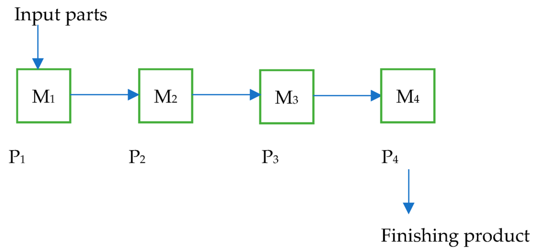
Figure 1 shows a flow shop scheduling process with four machines. The figure depicts four machines and four products. Each machine performs a single operation. The input parts enter the first machine and exit as finished products, labeled as P4.

In Figure 2, the flow shop scheduling process flowchart is presented. According to this process, the first step is to define the problem type and assumptions. Then, the number of jobs and machines, as well as the job sequence, should be determined. After the processing times are provided, a solution must be created using an appropriate algorithm. Once the schedule is generated, the makespan is calculated to reach the final result.

There are two classes into which flow shop scheduling problems may be grouped depending on the attributes of the machinery being used: those with buffer spaces and those where processing occurs continuously, without any interruptions between machines. The persistent execution of jobs without interruptions is known as the flow shop problem with no waiting time.

This matter is highly critical in industries such as food or metal production, where smooth and uninterrupted progression from beginning to end is absolutely essential for the production process [24].

The primary objective of this research is to investigate the m-machine flow shop problem, with a particular focus on minimizing the overall time required for completion. This is a crucial requirement, often referred to as the makespan objective.

This study examines scheduling situations involving many machines, with the goal of optimizing the total time needed to complete all jobs. This research provides useful insights into the topic of flow shop scheduling.

The ordered flow shop scheduling problem, initially introduced by Smith [8], represents a specialized subset of the classical flow shop scheduling problem characterized by specific structured properties of processing times. In the classical flow shop problem, the processing times are typically assumed to be independent across jobs and machines, with no inherent dependencies between them [23].

2.2. The Problem of Scheduling in Ordered Flow Shops

Two key conditions must be met by ordered flow shop problems. When comparing two jobs, A and B, which have fixed processing times, a crucial requirement is that, if job A takes less time to process on any machine than job B, then job A must also have an equal or shorter processing time than job B on all machines. This attribute guarantees a uniform sequence of processing durations for jobs A and B across several machines, establishing a fundamental feature in ordered flow shop issues [2].

Furthermore, in the context of ordered flow shop problems, a fundamental principle states that if a job has its jth shortest processing time on any machine, then every other job must also have its jth shortest processing time on the same machine. This condition emphasizes the significance of keeping a precise sequence across all jobs and machines involved in the flow shop scheduling problem. It ensures a constant and organized arrangement of processing times. The realization of these attributes contributes to the clearly defined framework and inherent qualities found in organized flow shop problems.

A sequencing approach can be used for jobs by arranging them in ascending order based on their processing times, provided that these two conditions are fulfilled. By strategically arranging the jobs, the original scheduling problem is transformed into an ordered flow shop problem, attempting to minimize the makespan and permutation schedules. This approach conforms to the prescribed sequence of processing times, which is in line with the core concepts of ordered flow shop issues. As a result, it facilitates the development of efficient and optimum scheduling solutions. This transformation enables a systematic and structured approach to addressing the problem, making it easier to create effective algorithms and procedures specifically designed for ordered flow shop settings.

Many flow shop sequencing problems have been studied in the literature [26]. Among the various instances, researchers have found that the classical (n × m), ordered (n × m), no-wait (n × m), and ordered no-wait (n × m) problems are the most interesting [2].

In the traditional problem, a key feature is the existence of unlimited intermediate storage spaces between machines, which means that there are no restrictions on the number of jobs that can be queued between consecutive units. Reddy and Ramamoorthy [27], in addition to Wismer [28], established a significant limitation called “no waiting”. They justified this change by establishing limitations that restrict or eliminate the queuing of jobs between machines.

Research on both the traditional (n × m) problem and a variant of the (n × m) problem without waiting goes beyond the makespan requirement to also include considerations of the mean flowtime criterion. Although it may not be possible to comprehensively achieve effective solution processes for these situations, there are some significant exceptions.

In the context of computational complexity, both of these issues are regarded as unsolvable. Nevertheless, it is feasible to create specific methods to deal with and reduce the computational difficulties linked to these issues, as proposed by Coffman [29]. These specific methods may provide useful insights and strategies to address the difficulties inherent in the classical and no-waiting flow shop sequencing problems, adding to the continuing discussion in the field of scheduling research.

Flow shop problems with the (n × m) ordered configuration have developed distinctive features in their processing times over time. Smith et al. [9] and Panwalkar et al.’s [30] contributions form the basis of this topic, highlighting the importance of taking into account particular characteristics associated with processing times.

Panwalkar and Woollam [31] studied the (n × m) ordered problem without waiting, with an emphasis on the makespan criterion. Throughout their research, they developed straightforward but effective techniques designed to deal with specific cases of this issue. Their study advances our knowledge of ordered flow shop problems, especially those involving the additional constraint of no waiting. It provides useful and efficient solution techniques for certain cases of the (n × m) ordered problem.

Smith [32] proved a crucial optimality finding for ordered flow shop problems. Specifically, in order to achieve optimal sequences, jobs must be arranged in either ascending or descending order in relation to their processing times. This ensures that the maximum processing time of each work instance is completed at the start or finish of the process. This realization gives rise to useful sequencing techniques. When each work instance takes the longest to process on the first machine, it is essential to prioritize arranging the jobs in descending order to achieve the most efficient arrangement. On the other hand, jobs should be arranged in ascending order to achieve the best schedules when the last machine experiences the longest processing time.

However, Smith et al. [32] proposed a technique aimed at decreasing the makespan in situations when the longest processing time is located on a middle machine. The best arrangement in this case is to arrange the jobs based on the processing times in ascending order first, and then to arrange the remaining jobs in reverse order. With its methodical approach to solving ordered flow shop problems and its ability to handle a wide range of machine-specific processing time distributions, this algorithm offers important insights into the best ways to sequence solutions for various problem scenarios.

Smith’s method produces 2ⁿ⁻¹ alternative sequences by following three steps. The first step is to arrange the jobs on the first machine in ascending order regarding their processing times. The second step is to assign the lowest-ranked job that is still unarranged to the array’s leftmost and rightmost empty spaces inside each subset of the sequence. We repeat Step 2 until each array has the first n-1 jobs allocated to it. Next, we assign the highest-ranked position to the open position. The third step is to evaluate the 2ⁿ⁻¹ sequences to obtain the makespan. Sequences that have the lowest makespans are regarded as optimal.

2.3. Utilizing Genetic Algorithms to Solve the Permutation Flow Shop Problem

Heuristic search techniques such as genetic algorithms, incorporating sophisticated stochastic search strategies, can provide nearly optimal results in complex circumstances [33]. These algorithms are extremely efficient in solving problems, particularly when dealing with large search areas, where conventional techniques may struggle to discover solutions effectively. Based on the fundamental principles of genetic inheritance and the mechanisms of natural selection, genetic algorithms (GAs) function by representing alternative solutions as chromosomes within the search space. The effectiveness of GAs depends on the specific formulation of the crossover and mutation operators used in each iteration. Therefore, correctly identifying these operators is a critical factor in determining the algorithm’s efficiency. GAs include inherent adaptability and exploration capabilities, which make them ideal tools in addressing complex optimization problems in several fields. Kumar et al. [34,35] also utilized a genetic algorithm to solve different flow shop problems.

When utilizing genetic algorithms (GAs) for problem-solving, the methodical approach entails several crucial phases. Initially, solutions that are feasible must be converted into chromosomes, presented as structures in the form of strings [33].

The initial stage of a typical genetic algorithm (GA) is to build a set of assumed or randomly generated solutions, known as chromosomes, to establish the initial population. The method advances through many sets of solutions, referred to as chromosomes, across multiple generations, intending to ultimately find the best possible solution for a particular problem. The suitability of each chromosome in every generation is determined by an objective function. In the context of flow shop scheduling problems, the fitness value of each chromosome is calculated as the inverse of the makespan.

Natural selection entails the selection of a certain set of chromosomes for reproduction, mostly depending on their degree of fitness. The reproductive success of each parent varies directly with its fitness level, and those with lower fitness levels are excluded. Once chromosomes have reproduced, genetic operators, including mutation and crossover, are used to create new chromosomes or offspring. The recently created chromosomes represent the succeeding generation, and this repetitive procedure persists until a termination condition is fulfilled. Genetic algorithms utilize a systematic technique to efficiently explore and exploit the solution space, resulting in the identification of optimal or near-optimal solutions for complicated problems.

The permutation flow shop problem entails the sequential processing of many jobs on a set of machines, following a predetermined order on each unit. This problem’s main goal is to determine the job sequence that takes the smallest amount of time to complete in total. This analysis focuses on a distinct assembly line situation within the topic of scheduling problems in permutation flow shops. This scenario involves a set of m separate jobs that need to be processed across a set of n different machines.

Importantly, all jobs must follow a consistent predetermined sequence on every machine, with their processing times preestablished and constant. The primary goal is to determine a sequence of jobs that results in the most efficient or shortest possible time for completion. This issue formulation is crucial in diverse manufacturing and production contexts, playing a significant role in optimizing the arrangement and sequencing of operations in flow shop environments.

The matrix displaying the processing time matrix for the problem is

P = (p_ij),      p_ij > 0,      i = 1, …, m      j = 1, …, n

Each machine is responsible for processing only one job at any given time. Moreover, each job is subjected to processing on just one machine. The objective of this problem is to set a job order with the aim of minimizing the makespan, i.e., minimizing the longest completion time among all jobs.

The objective is to minimize the maximum completion time, denoted as max_iC_i, where C_i represents the completion time for job i. This formulation focuses on optimizing the total production time by lowering the duration required for the last job to be completed.

The following traditional method can be used to successfully apply a genetic algorithm (GA) to the permutation flow shop problem. The fundamental components of a typical genetic algorithm are also described below.

The encoding scheme considers job sequences to be chromosomes. For example, a chromosome in a five-job scenario could be represented as [12543]. The order of jobs is indicated by this illustration, with Job 1 being processed on all machines first, followed by Job 2, Job 5, Job 4, and, lastly, Job 3 on all machines. An obvious and practical solution to the permutation flow shop problem is the encoding method.

Initial Population: N randomly generated job sequences constitute the initial population, where N is the population size.

Evaluation of Fitness Function: Natural selection, which favors the fittest individuals in evolution, is reflected in this function. It assigns a numerical number to each individual in the population to indicate their comparative excellence. Let r_i, represent the reciprocal of the makespan for each string in the population (with i = 1, …, N). The fitness value for string i is then given by f_i = r_i/∑_j r_j, making it proportional to r_i.

Reproduction: The chromosomes of the existing population are duplicated based on their individual fitness levels. The replication process involves selecting chromosomes in a random manner, with the likelihood of selection being based on their individual fitness ratings. In order to construct the next generation, there must be N × f _i instances of string i present in the gene pool. The mating pool is where the crossover and mutation operators are employed to produce the subsequent generation.

Crossover: The fundamental purpose of this procedure is to facilitate the exchange of information between parent chromosomes that are selected at random, leading to the production of offspring that are enhanced or improved. The crossover method involves the merging of genetic material from two parent chromosomes to produce offspring for the subsequent generation. The offspring inherit beneficial features from the parent chromosomes, with the goal of discovering superior gene combinations through genetic recombination [33].

Execution of Crossover: The execution of the crossover operation involves randomly selecting two parent chromosomes from the mating pool. They experience replication with a probability of 1 − p_c, where p_c is the likelihood of crossing.

Within the traditional genetic algorithm framework, a single-point crossover occurs between two parent chromosomes. To do this, a number k is selected randomly from the range 1 to l − 1, where l denotes the length of the string and is greater than 1. Swapping all characters starting from position k + 1 to l results in the creation of two distinct strings. It is worth mentioning that this encoding strategy has the potential to produce strings that are impossible to achieve. For example, in a situation where there are eight jobs and the parameter k is set to 3, the resulting strings after crossover could be [12345678] and [58142376].

This problem may give rise to potential solutions, such as [12342376] and [58145678], which are infeasible since they involve repetitive jobs. Hence, a change to the standard crossover approach is necessary. The initial modification involves replicating all characteristics of the chromosome from the first parent up to location k.

Mutation: During the crossover process, two distinct locations are selected at random within the chromosome, and the jobs placed at these positions are exchanged. Subsequently, the mutation operator is autonomously implemented on each offspring generated from the crossover process. The mutation operator applies a low probability, p_m, during its execution. Mutation is essential for expanding the range of possibilities in order to prevent selection and crossover from being too focused on a limited area. This precaution prevents the genetic algorithm from becoming trapped in a local optimum [33].

Termination Criterion: The maximum number of iterations at which the genetic algorithm (GA) will terminate is determined by this parameter.

The mathematical modeling of the genetic algorithm is given below [36].

Roulette, or proportional selection, is the primary method used in genetic algorithm selection. The goal of a crossover operation is to cross a single point and establish a fixed cross probability. The crossover probability is also fixed, and the mutation procedure is dependent on variation. The necessary parameters are established prior to implementing the genetic algorithm. The number of individuals in a population is represented by its size (M), which is typically between 20 and 100. In genetic operations, the numerical range of the evolution’s termination is often between 100 and 500. The variation probability p_m falls between 0 and 0.1, while the crossover probability p_c falls between 0.4 and 0.9. The ultimate solution, the solution time, and the genetic algorithm’s efficiency are all directly impacted by these four operating parameters.

The fitness value of individual i is represented by ${ƒ}_1$, and the population size is M. Equation (1) determines the likelihood that this person will be chosen. The method involves first calculating the fitness value ${ƒ}_1$ for each member of the population, where i = 1, 2… M.

$$Pi{\displaystyle \frac{{ƒ}_i}{{\sum }_{i=1}^M{ƒ}_i}}$$

(1)

Equation (2) computes the total fitness of all members of a population.

$$F={\sum }_{i=1}^M{ƒ}_i$$

(2)

Equation (3) calculates the likelihood of individual selection.

$$P_k={\displaystyle \frac{f_k}{{\sum }_{i=1}^M{f}_i}}, k= 1,2\dots \mathrm{M}$$

(3)

2.4. Reinforcement Learning

The production systems of today must contend with difficult circumstances, including customized mass manufacturing, fluctuating consumer demands, and other unpredictabilities. Reinforcement learning (RL) is frequently used to handle production planning and control issues, such as job shop scheduling (JSS), because of these intricacies and the dynamic nature of contemporary production systems [37].

In order to optimize an objective, JSS attempts to distribute a finite number of resources (machines) among several jobs. The jobs are subsequently handled in accordance with the schedule. RL can be used to address the job shop scheduling problem (JSSP). According to this machine learning paradigm, “learning agents are learning what to do—how to map situations to actions—in order to maximize a numerical reward signal” [38]. They learn how to accomplish their stated aim by interacting with their surroundings—that is, by acting and discovering the worth of their activity. However, the comprehension of its decision-making agents is hampered by (deep) RL’s black-box nature [39]. Explainable artificial intelligence (XAI)’s objective is to “produce details or reasons to make its functioning clear or easy to understand” [37].

2.5. Deep Reinforcement Learning

Scheduling problems are some of the most common challenges in the manufacturing sector, and manufacturing systems are essential to industrial production. The job shop scheduling problem (JSSP) is one of the most difficult combinatorial optimization and NP-hard scheduling problems among the different kinds of scheduling challenges [40].

Basic dispatching rules (DRs) were used by Jeong and Kim [41], O’Keefe and Kasirajan [42], and Shanker and Tzen [43]. Meanwhile, optimization algorithms, including tabu search (TS), simulated annealing (SA), genetic algorithms (GAs), particle swarm optimization (PSO), and ant colony optimization (ACO) (Brandimarte [44], Palmer [45], Kacem et al. [46], Ding and Gu [47], Sutton and Barto [48], and Jiang and Zhang [49]) are used in traditional methods for the FJSP.

GAs have been utilized by numerous researchers to tackle the FJSP because of their powerful search capabilities [40]. To overcome the FJSP, Ma et al. [40] suggested a DRL-assisted GA (DRL-A-GA) with the goal of minimizing the makespan. They created four FJSP-specific mutation operators and expressed the current population state of the GA using continuous state vectors. At several iterative stages, DRL helps the GA choose the appropriate parameters and evolutionary operators. These also appear in the literature as the latest alternative methods.

3. Materials and Methods

This section presents a comprehensive overview of the proposed approach, with a specific emphasis on PSA-GA, tailored to scheduling in an ordered flow shop. This method entails utilizing crossover and mutation processes to obtain a feasible solution characterized by convexity. The process is carefully defined in a sequential fashion, with each phase being clearly defined.

3.1. Pseudocode for Crossover Operations

The pseudocode for crossover operations is shown below: Crossover (Population)
{
Select Parent Index i randomly from the interval (1, Population.Size)
Select Parent Index j randomly from the interval (1, Population.Size)
Select random CutPoint from the interval (1, NoOfJobs) Create an empty new Child
For (k = 1 to CutPoint-1)
	Add Genek of the Parenti to the Child
End For For (k = CutPoint to NoOfJobs)
	If (Genek of the Parentj do not exist in the Child)
		Create a RandomValue from interval (0.1)
			If (RandomValue < 0.5)
				InsertFromLeft (Child, Parentj[Genek])
			Else
				InsertFromRight (Child, Parentj[Genek])
			End If
	End If
End For
For (k = CutPoint to NoOfJobs)
	If (Genek of the Parenti do not exist in the Child)
		Create a RandomValue from interval (0.1)
			if (randomValue < 0.5)
				InsertFromLeft (Child, Parenti[Genek])
			Else
				InsertFromRight (Child, Parenti[Genek])
			End If
	End If
End For
}

3.2. Pseudocode for Mutation Operations

The pseudocode for mutation operations is shown below: Mutation (Chromosome)
{
If (PeakGene is the first gene in the Chromosome)
	Select random index i from the interval [2, NoOfJobs]
	Remove Genei from the Chromose
	Insert Genei as the first Gene to the Chromosome
Else
	If (PeakGene is the first gene in the Chromosome)
		Select random index i from the interval [1, NoOfJobs-1]
		Remove Genei from the Chromose
		Insert Genei as the last Gene to the Chromosome
	Else
		Select random index i from the interval [1, PeakIndex)
		Select random index j from the interval (PeakIndex, NoOfJobs]
		Select the integer k randomly from {1,2,3}
		Remove Genei from the Chromosome
		Remove Genej from the Chromosome
			If (k==1)
				InsertFromLeft (Chromosome, Genej)
				InsertFromLeft (Chromosome, Genei)
			End If
			If (k==2)
				InsertFromRight (Chromosome, Genei)
				InsertFromRight (Chromosome, Genej)
			End If
			If (k==3)
				InsertFromLeft (Chromosome, Genej)
				InsertFromRight (Chromosome, Genei)
			End If
	End If
End If
}
InsertFromLeft (Chromosome, Gene)
{
If (The process time of the Gene > The process time of the PeakGene)
	Insert the Gene to immediately after the PeakGene
Else
	For (k = 1 to PeakIndex)
		If (The process time of the Genek ≥ The process time of the Gene)
			Insert Gene to Index k
			Break For
		End If
	End For
End If
}
InsertFromRight (Chromosome, Gene)
{
If (The process time of the Gene > The process time of the PeakGene)
	Insert the Gene to immediately after the PeakGene
Else
	For (k = NoOfJobs down to PeakIndex)
		If (The process time of the Genek ≥ The process time of the Gene)
			Insert Gene to Index k + 1
			Break For
		End If
	End For
End If
}

3.3. Steps of the Proposed Method

Data Initialization: The initial step of the proposed approach is to generate a matrix that specifies the times of jobs on various machines in a specific order. This matrix structure has two essential qualities that are typical of ordered flow shop problems. We assigned random values ranging from 0 to 999 to the elements of the matrix. The software obtained essential information regarding the number of jobs and available machines, specifically including instances with 10 jobs and 15 machines or 30 jobs and 10 machines. The proposed solution addresses issues related to job amounts ranging from 20 to 800 and machine quantities ranging from 5 to 60.

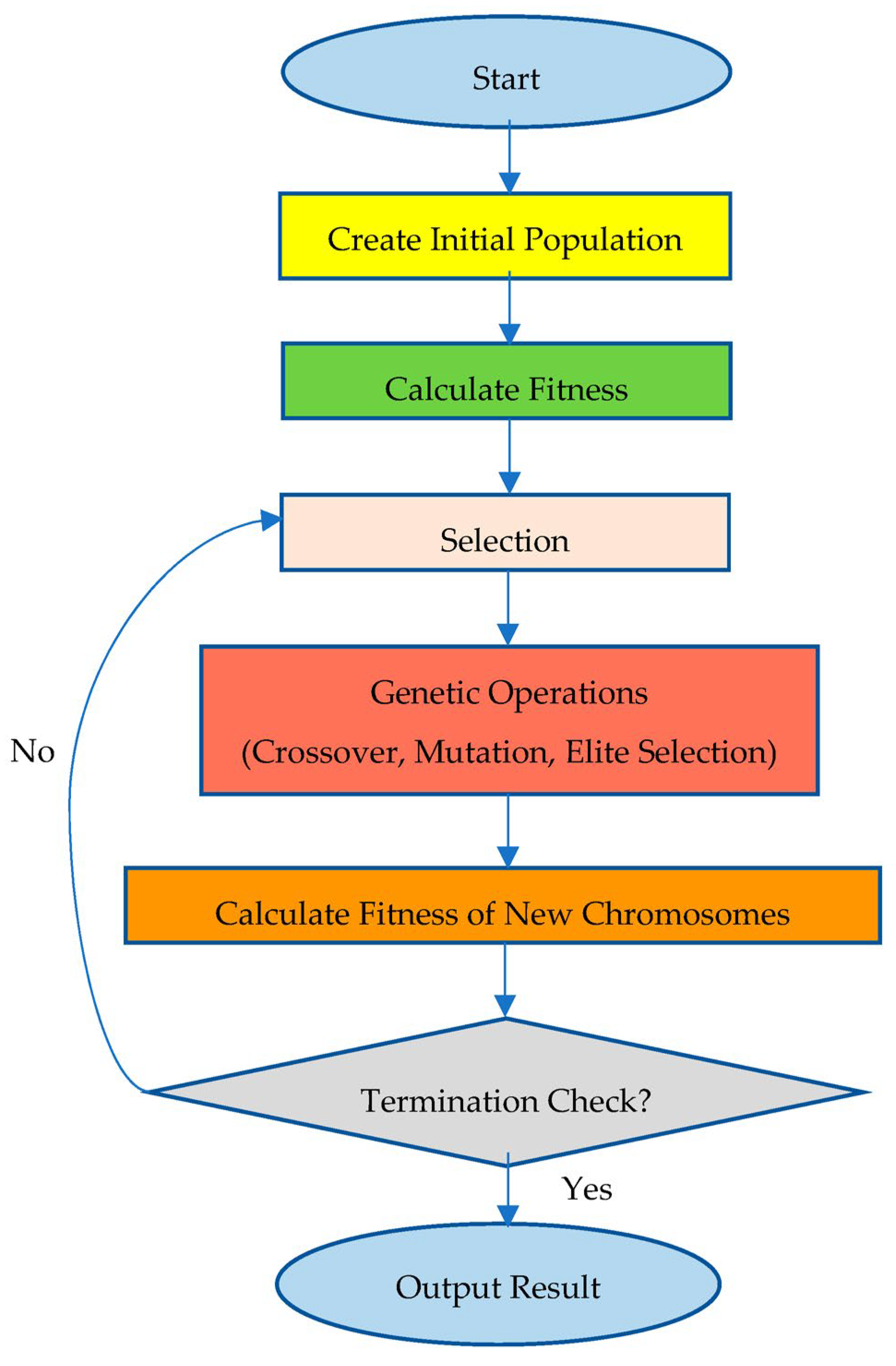
The proposed genetic algorithm flowchart is shown in Figure 3.

Population Size Determination: The determination of the population size has emerged as an important criterion that requires careful consideration in this step.

Initial Population: In the initial population, chromosomes are first created randomly (Figure 4 and Figure 5) and then modified to obtain a pyramid shape, defined as in Smith [8] as follows.

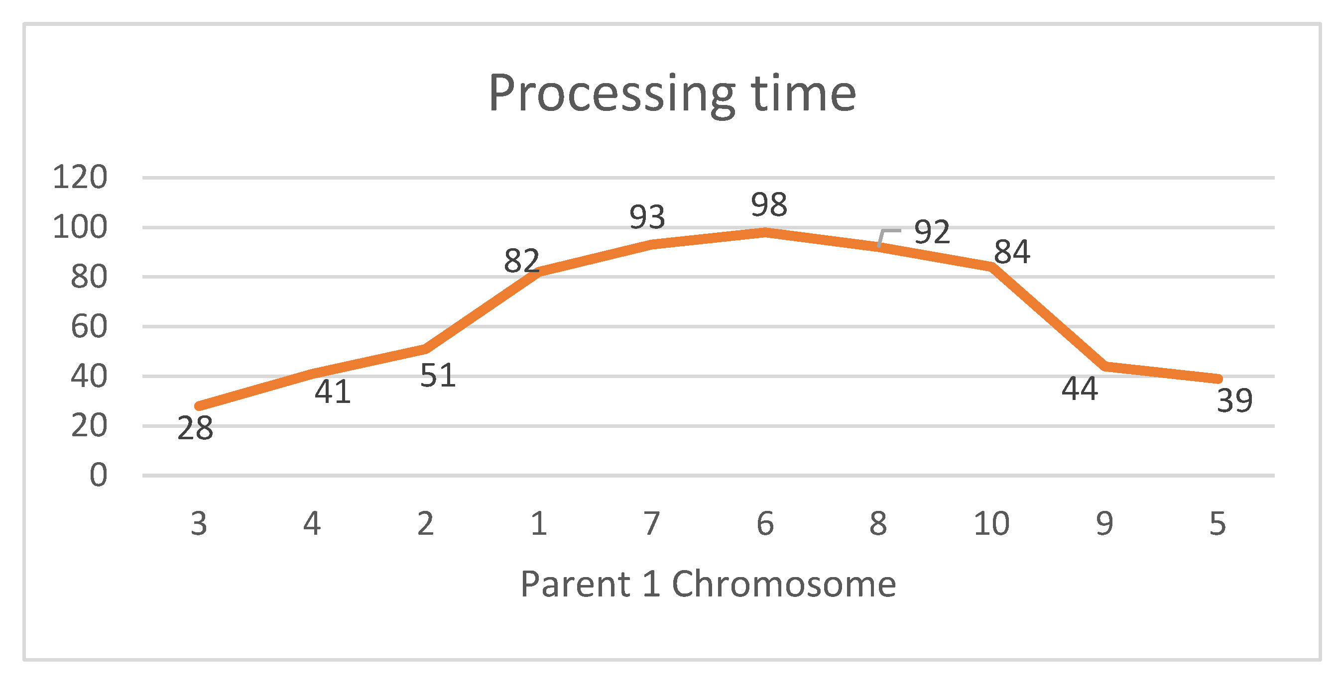
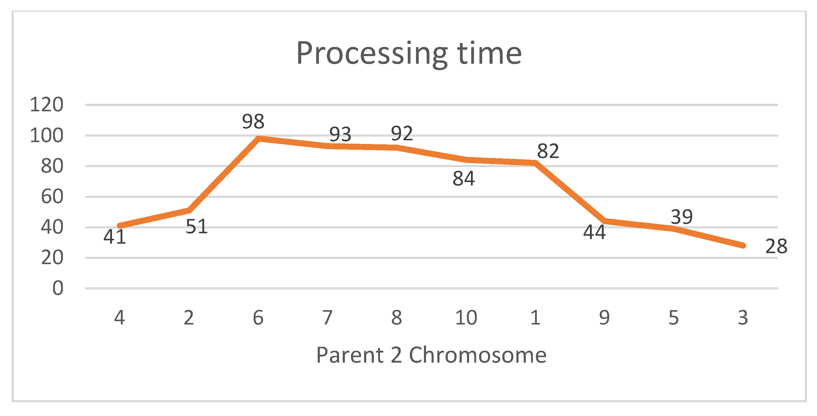
In the chromosome, first, the job with the largest processing time is selected and copied to the same position. Then, the jobs on the left of the selected job are ordered based on their processing times in non-decreasing order, and the jobs on the right of the selected job are ordered based on their processing times in non-increasing order, as seen in the following chromosome (Figure 6 and Figure 7).

There are two specific cases in creating the pyramid shape of the chromosomes. The first specific case has the longest job in the first position. In this case, all jobs will be moved to the right-hand side of the longest job in non-increasing order regarding their processing times.

The second specific case has the longest job in the last position. In this case, all jobs will be moved to the left-hand side of the longest job in non-decreasing order regarding their processing times.

Crossover Operator: In the proposed pyramidal genetic algorithm, one-point crossover with a modification to retain the pyramid shape is used. This modified one-point crossover operator works as follows.

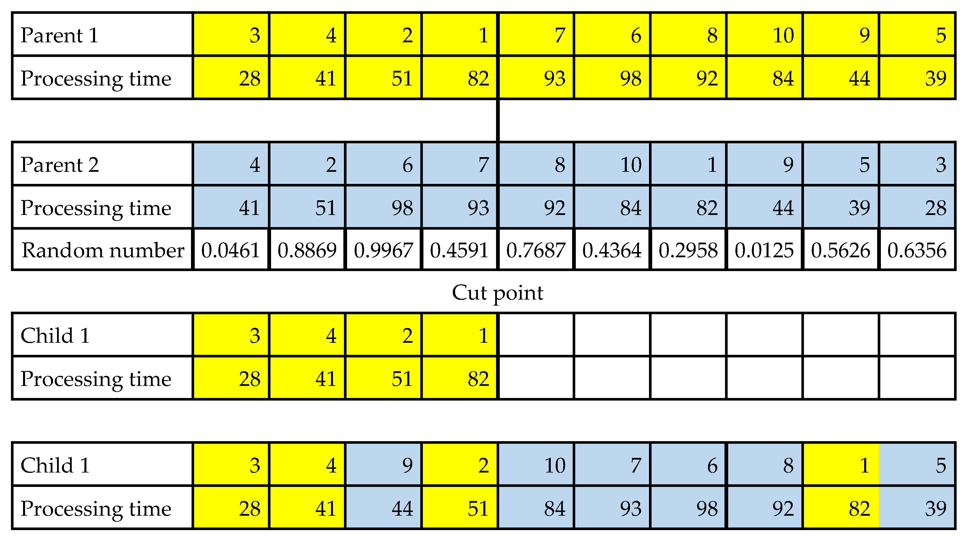
First, two parent chromosomes are selected by using roulette wheel selection. Then, to create the first child, a cut point is selected randomly. From the first parent, the first part of the chromosome is copied to the first child.

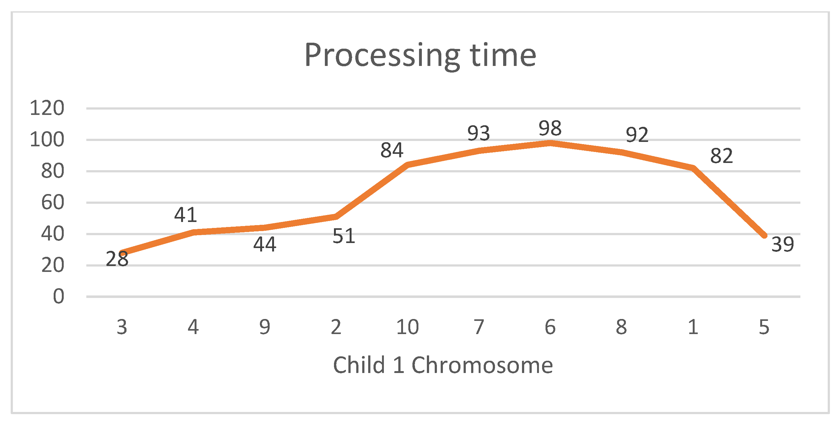
Then, the remaining part of the first child is taken from the second part of the second parent one at a time and inserted with a 50% probability, either from the left-hand side or from the right-hand side of the job, until the selected job’s processing time passes those of all jobs with shorter processing times (on the left-hand side by observing non-decreasing processing times or on the right-hand side by observing non-increasing processing times). When the end of the second parent chromosome is reached, the selection continues from the beginning of the second parent. An illustration of this processes can be seen in Figure 8, Figure 9, Figure 10 and Figure 11.

As can be seen in Figure 8, the first part of parent chromosome 1 is copied to the first child. Then, starting after the cut point, the jobs are taken from the second parent and added to the first child as follows: first, Job 8 is selected (since its random number is 0.7687 and greater than 0.5) and inserted from the right-hand side until its processing time passes the processing time of Job 1. Similarly, the rest of the jobs will be selected one at a time and inserted into the child chromosome if they are not already in the child chromosome, as can be seen in Figure 8.

The proposed crossover steps are shown in

Table 1. Proposed crossover steps.

Selected Job	Random Number	Direction of Placement	Placement Between Jobs
8	0.7687	From right	Between Job 2 and Job 1
10	0.4364	From left	Between Job 2 and Job 8
1	-	Already exists
9	0.0125	From left	Between Job 4 and Job 2
5	0.5626	From right	After Job 1
3	-	Already exists
4	-	Already exists
2	-	Already exists
6	0.9967	From right	Between Job 10 and Job 8
7	0.4591	From left	Between Job 10 and Job 6

. It illustrates where each job will be placed according to the random number.

Mutation Operator: Three different mutation operators are used in the proposed PGA. These mutation operators are used with equal probabilities.

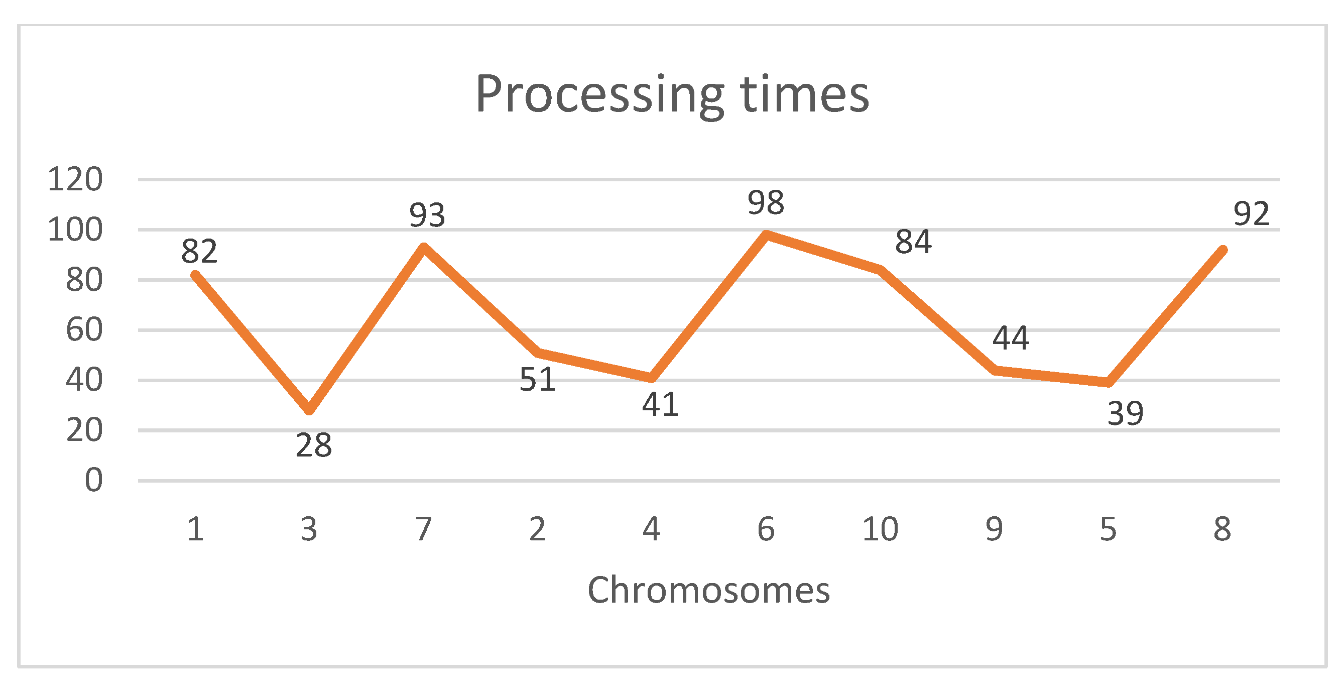
Mutation Operator 1: In this mutation operator, a random job is selected from the left-hand side of the job with the longest processing time and inserted at the right-hand side of the job with the longest processing time to retain the pyramid shape. The chromosomes and the processing times are presented in Figure 12 and additionally visualized in Figure 13.

Regarding the chromosome after mutation operator 1, Job 9 is selected and inserted at the right-hand side of the job with the longest processing time, namely Job 6, retaining the pyramid shape. The chromosomes and the processing times after mutation operator 1 are presented in Figure 14 and additionally visualized in Figure 15.

Mutation Operator 2: In this mutation operator, a random job is selected form the right-hand side of the job with the longest processing time and inserted at the left-hand side of the longest job to retain the pyramid shape. The chromosome and the processing times are shown in Figure 16 and are also illustrated in Figure 17.

Regarding the chromosome after mutation operator 2, Job 5 is selected and inserted at the left-hand side of the job with the longest processing time, namely Job 6, retaining the pyramid shape. The chromosome and processing times are provided in Figure 18 and further depicted in Figure 19.

Mutation Operator 3: In this mutation operator, two random jobs are selected—one from the left-hand side and the other from the right-hand side of the job with the longest processing time—and inserted at the opposite sides of the job with the longest processing time to retain the pyramid shape. Figure 20 and Figure 21 provide a graphical representation.

Regarding the chromosome after mutation operator 3, Job 2 is selected from the left-hand side and inserted at the right-hand side, and Job 8 is selected from the right-hand side and inserted at the left-hand side of the job with the longest processing time, namely Job 6. Figure 22 and Figure 23 illustrate these steps.

Termination Criteria Definition: The termination criteria were precisely defined for every member of the ordered matrix. The population size and termination criteria for the problem are specified in

Table 2. Parameters of proposed genetic algorithm.

Job, n	Pop Size	Time	Mutation	Crossover	Elitism
<300	2n	n	40%	60%	50%
≥300	2n	2n
≥500	N	3n

, with “n” being the number of jobs. The values in the table were carefully determined and selected using a design of examinations. In the conducted experiment, the population sizes were set as n and twice the value of n. The study employed mutation rates of 20%, 30%, and 40%; crossover rates of 60%, 70%, and 80%; and elitism values of 30%, 40%, and 50%, which were consistent with the findings of previous studies. A Taguchi analysis was conducted to determine the optimal parameters. In the Taguchi method, an orthogonal array is utilized to design experiments. This array represents a subset of the full factorial design trials, capturing the essential information required for analysis. Taguchi categorizes factors into two main groups: controllable factors and uncontrollable noise factors. These factors are employed to create test problems.

If a full factorial design is applied, then 27 combinations (three controllable factors with three levels for each) should be performed. Thus, 27 × 60 × 5 = 8100 instances should be solved in total. The Taguchi method suggests an orthogonal array L9 for an experiment with three factors, with each of them in three levels.

The method recommends analyzing variation using the signal-to-noise ratio (S/N). Since the goal is to minimize the objective function value, the appropriate S/N ratio formula is suggested as in Equation (4):

$$S/N=-10\times {\log }_{10}\left({\displaystyle \frac{1}{n}}{\sum }_{i=1}^n{y}_i^2\right)$$

(4)

This ratio reflects the variation in the response variable, where the signal represents the desirable value and the noise signifies the undesirable value, such as the standard deviation.

Table 3. Parameters and S/N ratios.

Parameter	Mutation	Crossover	Elitism	S/N Ratio
1	0.20	0.60	0.30	−105.9716590
2	0.20	0.60	0.40	−105.9716537
3	0.20	0.60	0.50	−105.9716364
4	0.20	0.70	0.30	−105.9716711
5	0.20	0.70	0.40	−105.9716921
6	0.20	0.70	0.50	−105.9716828
7	0.20	0.80	0.30	−105.9717025
8	0.20	0.80	0.40	−105.9716920
9	0.20	0.80	0.50	−105.9716722
10	0.30	0.60	0.30	−105.9716246
11	0.30	0.60	0.40	−105.9715927
12	0.30	0.60	0.50	−105.9716276
13	0.30	0.70	0.30	−105.9716472
14	0.30	0.70	0.40	−105.9716364
15	0.30	0.70	0.50	−105.9716046
16	0.30	0.80	0.30	−105.9716451
17	0.30	0.80	0.40	−105.9716325
18	0.30	0.80	0.50	−105.9716192
19	0.40	0.60	0.30	−105.9715882
20	0.40	0.60	0.40	−105.9715982
21	0.40	0.60	0.50	−105.9716038
22	0.40	0.70	0.30	−105.9716255
23	0.40	0.70	0.40	−105.9716141
24	0.40	0.70	0.50	−105.9716415
25	0.40	0.80	0.30	−105.9716442
26	0.40	0.80	0.40	−105.9716060
27	0.40	0.80	0.50	−105.9716136

shows the S/N ratios of the 27 parameters.

According to

Table 4. Factors and their levels.

Analysis	Mutation	Crossover	Elitism
Level 1	−105.97167	−105.97162	−105.971645
Level 2	−105.97163	−105.97165	−105.971635
Level 3	−105.97162	−105.97165	−105.971634
Delta	0.0000585	0.0000270	0.0000118
Rank	1	2	3
Best Value	0.40	0.60	0.50

, the best values for mutation, crossover, and elitism are 0.4, 0.6, and 0.5, respectively.

Once the ordered matrix was created, the subsequent job involved generating parents. The parents were randomly selected and a technique was used to identify the peak. Afterward, the parents were arranged in ascending order from the beginning to the highest point and in descending order from the highest point to the end. Notably, it was verified that the matrix possessed only a single peak.

During the third phase, the crossover operation was executed to produce offspring by combining the genetic material of the chosen parents. The parents underwent stochastic division into two parts, with a 60% likelihood, and the division did not necessarily occur at the halfway point. The initial portion of the primary parent was replicated, while the latter section of the secondary parent was assimilated in accordance with the directives provided in the subsequent phase. This principle necessitates organizing the jobs in ascending order until the highest point is reached and subsequently arranging them in descending order. A crucial aspect that was carefully taken into account during the implementation of the crossover operation was the continuation of a singular peak in the matrix.

In the fourth stage, the mutation process involved the random selection of two elements while keeping the rest unchanged. The selected elements were relocated in accordance with the rule established in the second step, with a probability of 40%. This rule requires the arrangement of jobs in ascending order until reaching the peak; thereafter, they occur in descending order. The mutation process involved three separate scenarios: reciprocal displacement, both on the left side, and both on the right side. The parental candidate selection approach employed the roulette wheel selection technique, which entailed selecting two numbers at random and thereafter selecting parents whose combined fitness values closely matched these numbers. It is crucial to emphasize that the fitness values were evaluated by taking the reciprocal of the C_max values of the parents.

The final stage used elitism to create a new population, which represented the solution. This approach involved selecting the top 25% of individuals from the existing population and an additional 25% from the offspring population, representing a total of 50% of the new population. The other half of the new population comprised individuals from both the current population and the offspring population who were not chosen in the previous step.

4. Results

The effectiveness of the suggested methodology was evaluated across various termination criteria and mutation rates and varied numbers of machines and jobs. The technique was executed utilizing the C# programming language on Visual Studio 2019 Community Edition Version 16.9.4. (Microsoft Corporation, Redmond, WA, USA). Here, we describe a specific instance and its corresponding results.

Table 5. Matrix arranged in order.

J/M	M1	M2	M3	M4	M5
J1	2	34	9	18	14
J2	28	62	40	56	52
J3	3	41	13	28	17
J4	39	90	53	79	65
J5	48	104	68	94	70

shows the ordered matrix created using computer processes that employed random values based on the guidelines explained in this study.

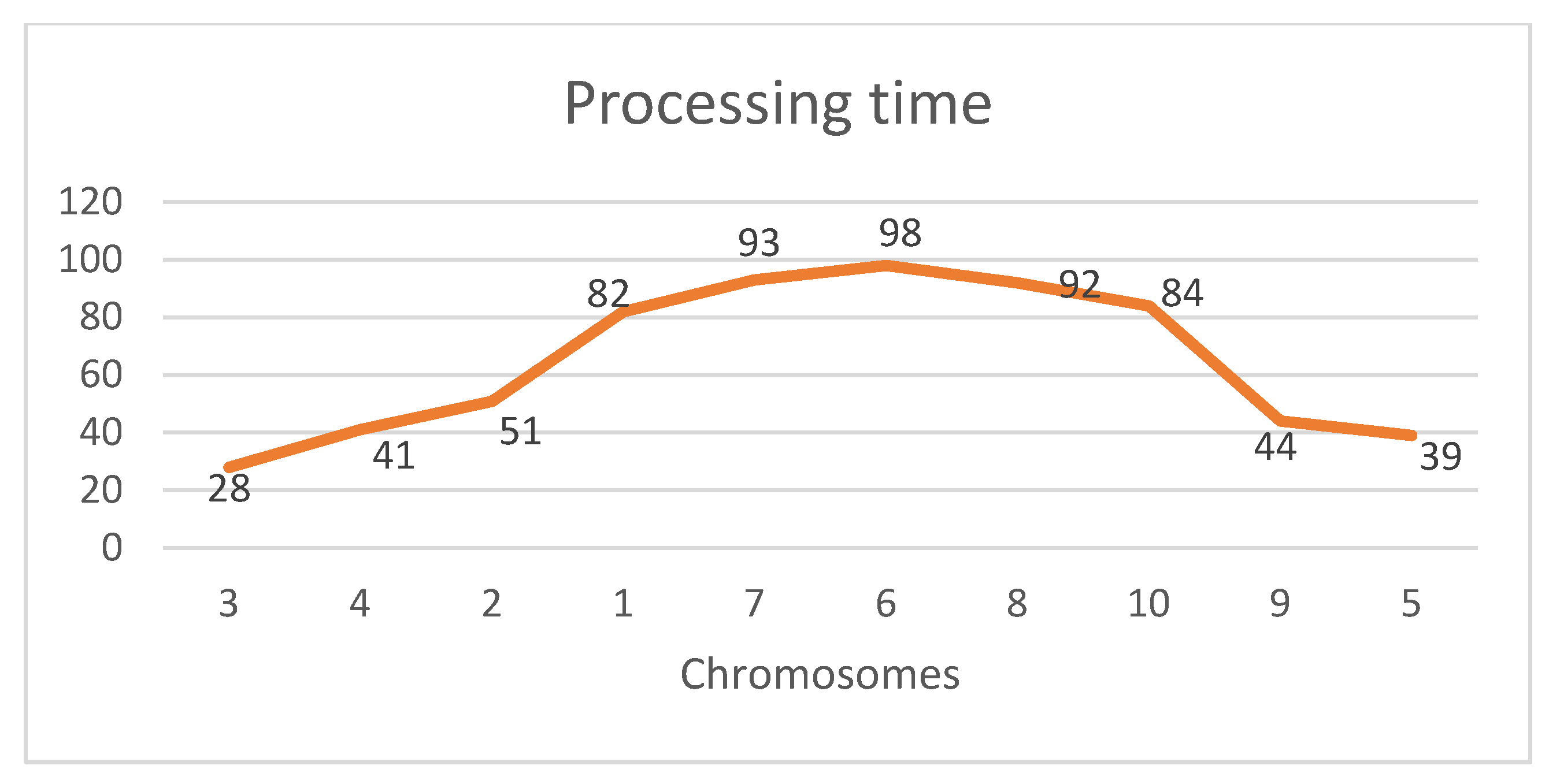
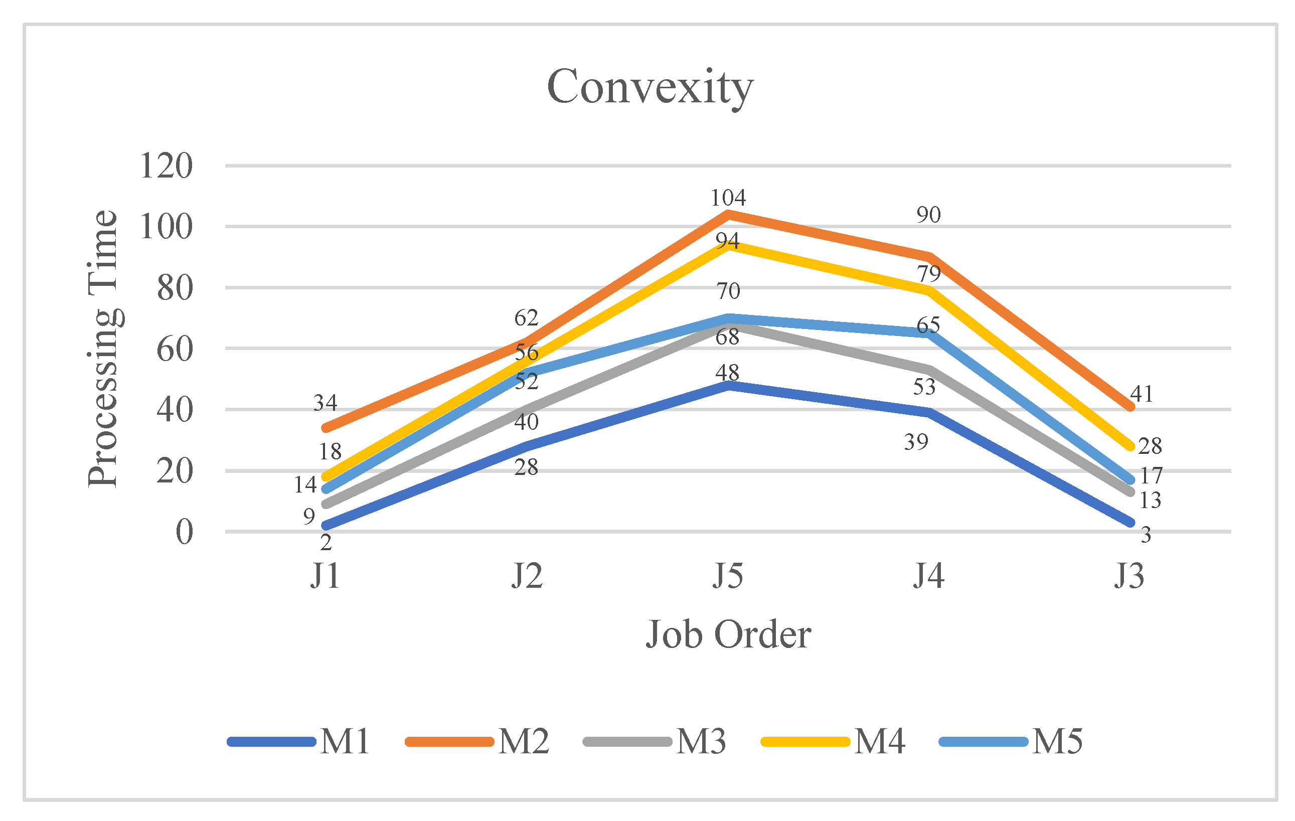
The lowest achieved number, 525, was the best fitness value for the optimal solution to this issue instance. Consequently, [J₁, J₂, J₅, J₄, J₃] was found to be the ideal job sequence linked to this fitness value.

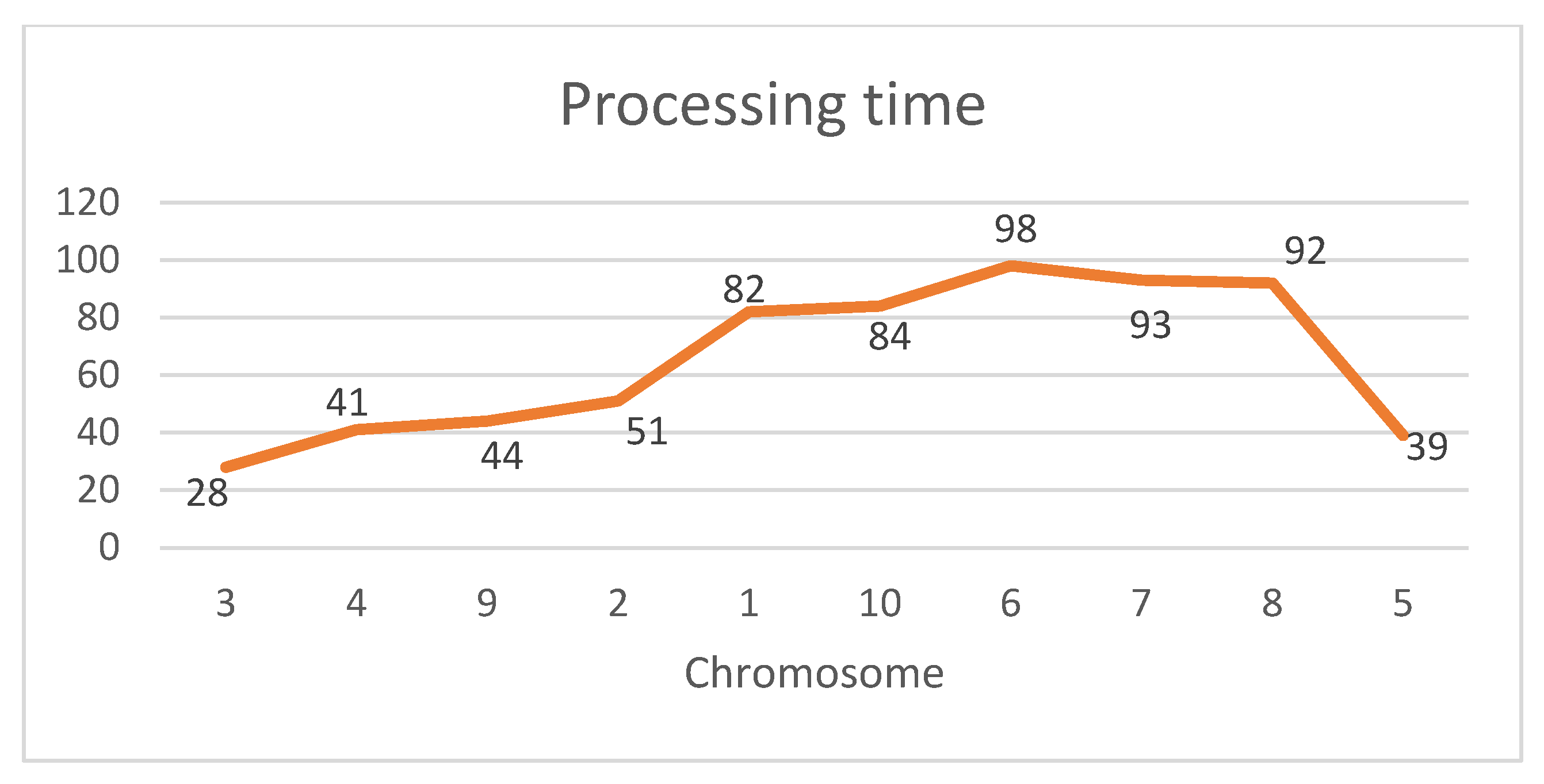
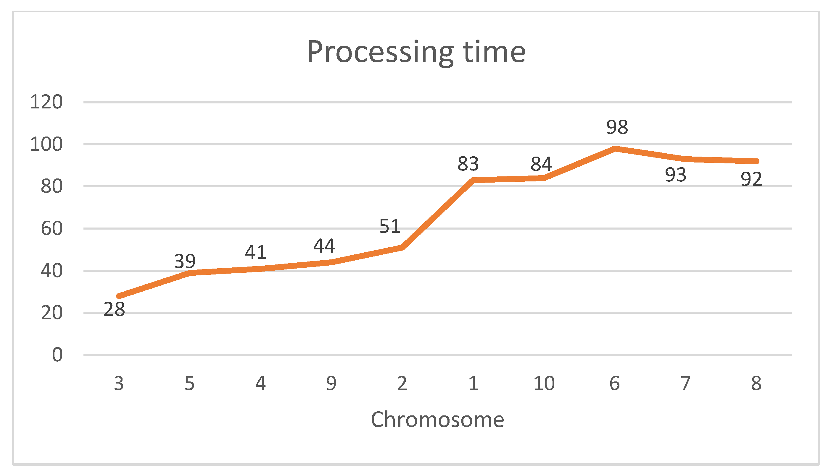
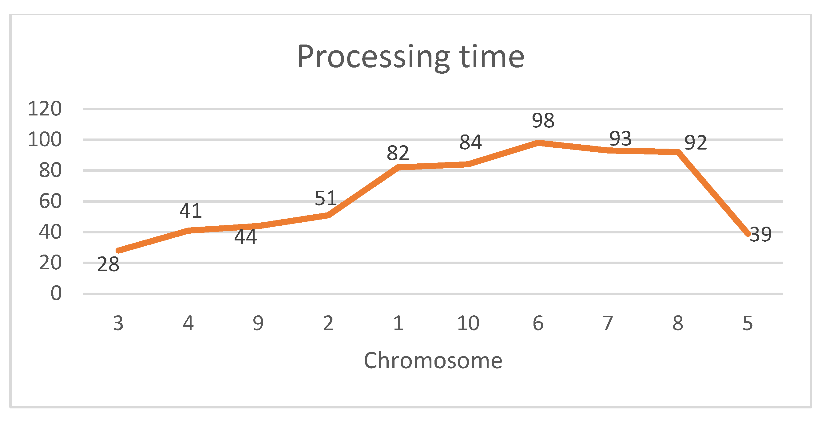
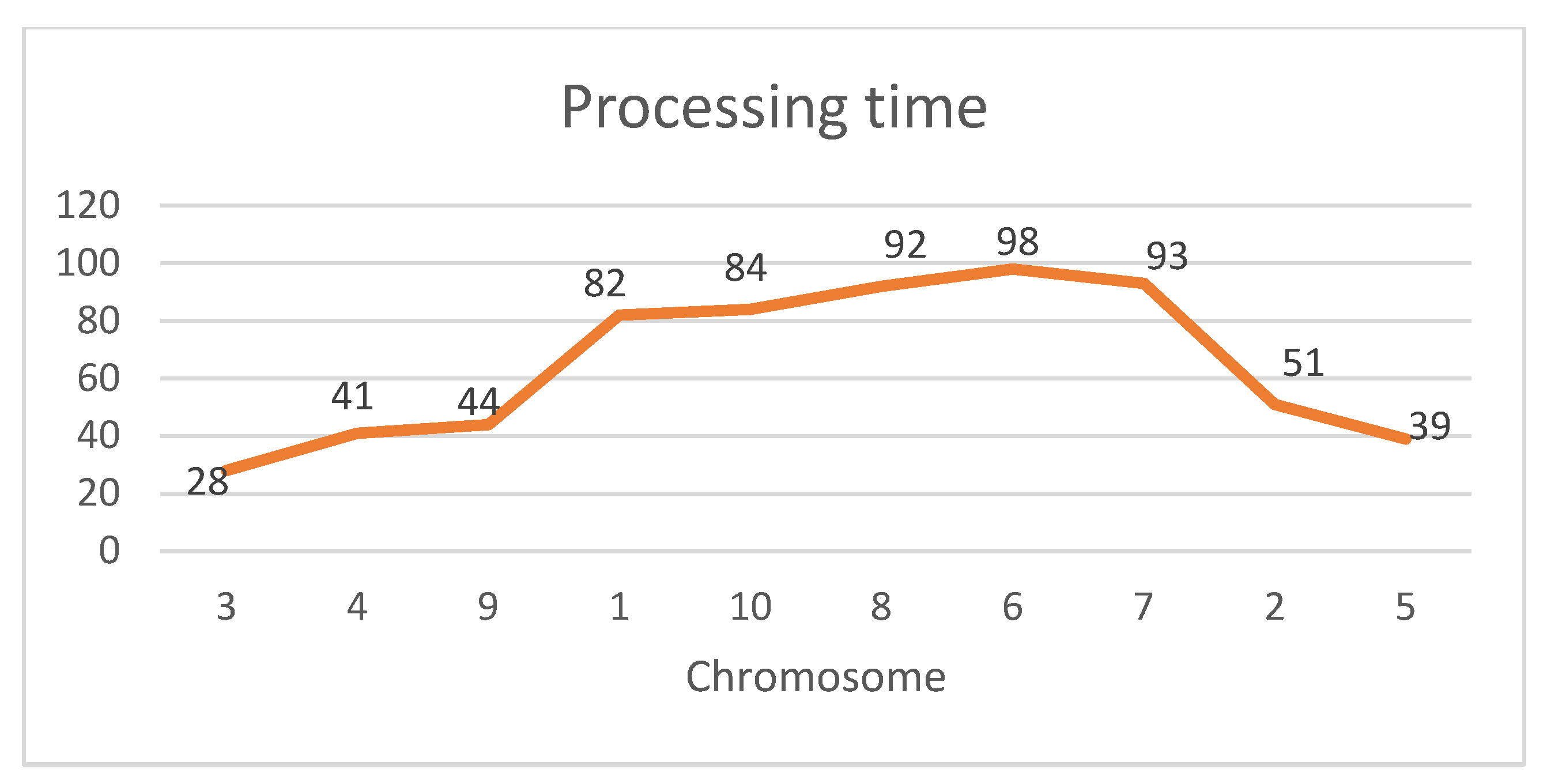
Figure 24 clearly demonstrates the convex nature of the generated result. The graphic depicts the processing times of individual machines, organized based on the most efficient work sequence. The graphic clearly shows a convex pattern, with an initial increase and subsequent decrease in the processing times, confirming the fundamental convex relationship in the solution. When examining the graph from beginning to end, it is also possible to observe a form of symmetry. In the sequence, jobs up to the longest job are ordered according to the SPT rule, while jobs after the longest job are ordered according to the LPT rule, creating a type of symmetry. According to Smith, this type of symmetry is necessarily present in the optimal schedule.

The experiment entailed creating processing times between 0 and 999. For each problem size, such as 10 jobs and 5 machines, five distinct instances were executed five times to obtain average makespan values.

Every computational experiment was carried out on a PC (Dell Technologies Inc., Round Rock, TX, USA) with an 8 GB RAM-equipped Intel^® CoreTM i7-6500U processor (Intel Corporation, Santa Clara, CA, USA) operating at 2.60 GHz. The Windows 10 Home OS was the operating system used in the trials.

The proposed method takes a methodical approach, starting by placing jobs in ascending order based on how long they take to process. Then, these jobs are sequentially added one at a time to the first and last empty slots in the array. This approach yields a total of 2ⁿ⁻¹ arrays in a scenario with n jobs.

Then, each array’s makespan and processing time are calculated, making it possible to determine which arrays are best suited based on certain optimization criteria. This procedure guarantees a thorough investigation of the solution space to find configurations that produce better results in terms of the processing time and makespan.

4.1. Instance and Set Generation

Currently, there is just one set of published benchmark examples available for the ordered flow shop scheduling problem, based on the most up-to-date information. Nevertheless, the current values in this study exhibit a lack of variety as they are closely grouped together. As a result, we have created supplementary benchmark problems available for this topic, aiming to offer a wider range of difficult benchmark problems. The reason for this is that, when the current datasets undergo changes, they yield comparable results for all techniques mentioned in the literature.

The benchmark examples in our database have a wide range, spanning from 5 to 60 machines and 20 to 800 jobs. The dataset has 39 combinations labeled as (n, m), with examples such as (20, 5), (30, 10), (50, 20), (75, 60), (100, 40), (200, 60), (300, 40), (500, 20), (700, 60), and various others. A total of 195 instances were generated by generating five examples for each combination.

In order to facilitate the analysis, we classified the occurrences into three groups: small (S), medium (M), and large (L). The S set consisted of instances containing 20 to 75 jobs, the M set included examples containing 100 to 500 jobs, and the L set comprised instances containing 600 to 800 jobs.

4.2. Parameters of Genetic Algorithm

Table 3 shows the parameters utilized in PSA-GA. Significantly, if the job size is zero or larger, the population size is set to double the value of n, and the termination criteria are determined by n, which reflects the number of jobs. Uniform settings for mutation, crossover, and elitism were consistently utilized for all problem settings.

The parameter values were carefully established and selected using a systematic design of experiments, as described in Section 3.3.

4.3. Comparison of the Proposed Method and Other Methods

The proposed approach was tested using four benchmark methods, with the comparison criteria focused on the number of best solutions obtained (N_BEST) and the average relative percentage deviation (ARPD).

The level of excellence of the results is assessed through the relative percentage deviation (RPD), calculated as ${\displaystyle \frac{z-\mathrm{z}\ast }{\mathrm{z}\ast }}\times 100$, where z represents the algorithm’s objective function value (makespan), and z* is the best-known objective function value for the specific instance. The ARPD is calculated by taking the average of the RPDs for different groups of instances. Each instance has been solved five times, and the stated results reflect the mean of these five iterations.

Table 6. Comparison of algorithms on S-sized problems.

Problem Size (n-m)	PSA-GA		NEH		Pair Insert		ILS+Pair Insert		PSA-TS
	NBEST	ARPD	NBEST	ARPD	NBEST	ARPD	NBEST	ARPD	NBEST	ARPD
20-5	5	0.0000	0	1.5839	0	1.4015	1	0.0748	4	0.0194
20-10	5	0.0000	0	0.9368	0	0.7372	4	0.0015	5	0.0000
20-20	5	0.0000	0	0.4499	0	0.3459	5	0.0000	4	0.0010
30-5	4	3.9810	0	11.1357	0	10.7289	0	4.2543	3	0.0019
30-10	4	0.0013	0	1.3062	0	1.0292	3	0.0131	5	0.0000
30-20	3	0.0019	0	0.8772	0	0.5043	1	0.0125	5	0.0000
40-5	3	0.0026	0	0.5388	0	0.4017	0	0.0473	4	0.0016
40-10	3	0.0066	0	0.7835	0	0.6968	0	0.0161	5	0.0003
40-20	1	0.0208	0	0.6186	0	0.4394	0	0.0524	4	0.0011
50-5	5	0.0004	0	0.9542	0	0.7510	0	0.1982	3	0.0049
50-10	2	0.0078	0	0.8894	0	0.7670	0	0.0902	3	0.0043
50-20	3	0.0026	0	0.7025	0	0.5168	0	0.0286	2	0.0036
75-20	4	0.0013	0	0.8094	0	0.5488	0	0.0339	3	0.0024
75-40	4	0.0003	0	0.3320	0	0.2606	0	0.0118	2	0.0016
75-60	3	0.0037	0	0.5513	0	0.5042	0	0.1210	2	0.0015
Total	54	0.0512	0	22.4694	0	19.633	14	4.9559	54	0.0434

presents the results of the five techniques (PSA-GA, NEH, pair insert method, ILS method, and PSA-TS) for the benchmark S instances.

Table 7. Comparison of algorithms on M-sized problems.

Problem Size (n-m)	PSA-GA		NEH		Pair Insert		ILS+Pair Insert		PSA-TS
	NBEST	ARPD	NBEST	ARPD	NBEST	ARPD	NBEST	ARPD	NBEST	ARPD
100-20	5	0.0000	0	1.2497	0	1.1745	0	0.8365	0	1.0488
100-40	4	0.0003	0	0.3568	0	0.2321	0	0.0142	2	0.0027
100-60	2	0.0017	0	0.3490	0	0.2661	0	0.0136	3	0.0007
200-20	4	4.3718	0	4.7984	0	4.7425	0	4.4286	1	0.0023
200-40	4	0.0001	0	0.5324	0	0.3564	0	0.0193	2	0.0167
200-60	5	0.0000	0	0.2447	0	0.1785	1	0.0079	1	0.4692
300-20	4	0.0002	0	0.2846	0	0.2297	0	0.0750	2	0.0064
300-40	4	0.0001	0	0.2345	0	0.1769	0	0.0161	2	0.0057
300-60	5	0.0000	0	0.2152	0	0.1659	0	0.0079	1	0.0220
400-20	4	0.0005	0	0.3866	0	0.3155	0	0.0331	1	0.0037
400-40	3	0.0004	0	0.4282	0	0.2759	0	0.0480	2	0.0080
400-60	2	0.0006	0	0.2950	0	0.2298	0	0.0079	4	0.0011
500-20	1	0.0021	0	0.4207	0	0.3023	0	0.0743	5	0.0000
500-40	2	0.0008	0	0.2847	0	0.2456	0	0.0526	3	0.0025
500-60	3	0.0003	0	0.2335	0	0.1710	0	0.0125	2	0.0023
Total	52	0.0074	0	10.3139	0	9.0627	1	5.6476	31	1.5921

displays the results for the benchmark M cases, whereas

Table 8. Comparison of algorithms on L-sized problems.

Problem Size (n-m)	PSA-GA		NEH		Pair Insert		ILS+Pair Insert		PSA-TS
	NBEST	ARPD	NBEST	ARPD	NBEST	ARPD	NBEST	ARPD	NBEST	ARPD
600-20	3	0.0006	0	0.3260	0	0.2766	0	0.0556	2	0.0046
600-40	4	0.0007	0	0.4329	0	0.3513	0	0.0587	1	0.0088
600-60	5	0.0000	0	0.3043	0	0.2133	0	0.1000	0	0.0620
700-20	5	0.0000	0	0.2274	0	0.2018	0	0.0367	1	0.0361
700-40	5	0.0000	0	0.2525	0	0.1924	0	0.0603	0	0.0355
700-60	5	0.0000	0	0.2582	0	0.2157	0	0.0292	0	0.0846
800-20	5	0.0000	0	0.2218	0	0.1821	0	0.0684	0	0.0699
800-40	5	0.0008	0	0.2091	0	0.1840	0	0.0377	0	0.1286
800-60	5	0.0015	0	0.1966	0	0.1594	0	0.0090	1	0.2281
Total	42	0.0036	0	2.4289	0	1.9767	0	0.4556	5	0.6583

shows the results for the benchmark L instances. In Table 6, the comparative performance of various methods is illustrated. Both PSA-GA and PSA-TS achieve the optimal solution in 54 instances. In contrast, the ILS method attains the best solution 14 times, while the NEH and pair insert methods do not achieve the optimal solution in any of the cases. Furthermore, when comparing the average relative percentage deviation (ARPD) of PSA-GA and PSA-TS, PSA-GA demonstrates superior performance, exhibiting the lowest ARPD.

As evidenced by Table 6, which details the comparison of the five algorithms applied to S-sized problems, PSA-GA consistently outperforms the others. Thus, based on this analysis, PSA-GA is identified as the most effective approach.

Table 7 presents a comparison of the five algorithms applied to M-sized problems. The data indicate that PSA-GA attains the optimal solution 52 times, outperforming PSA-TS, which achieves the best solution 31 times. The remaining algorithms fall significantly short of these results, failing to approach the performance of PSA-GA and PSA-TS. Additionally, when comparing the average relative percentage deviation (ARPD) of PSA-GA with that of the PSA-TS method, PSA-GA exhibits exceptional performance, demonstrating superior ARPD values.

According to Table 8, in terms of N_BEST or ARPD, none of the other algorithms approached the performance of PSA-GA. PSA-GA has thus clearly demonstrated its superior efficacy in handling large problems.

Table 9. Evaluation metrics (N_BEST and ARPD) for the PSA-GA, NEH, pair insert, ILS, and PSA-TS methods on the four benchmark sets.

Metric	Benchmark	PSA-GA	NEH	Pair Insert	ILS+Pair Insert	PSA-TS
NBEST	S	53	0	0	14	54
	M	51	0	0	1	32
	L	42	0	0	0	5
	Sum	146	0	0	15	91
ARPD	S	4.0302	22.4694	19.6333	4.9560	0.0435
	M	4.3790	10.3140	9.0627	5.6477	1.5922
	L	0.0036	2.4289	1.9767	0.4556	0.6583
	Average	2.8043	11.7374	10.2242	3.6864	0.7646

presents a comprehensive overview of the computational results obtained from the five methodologies. PSA-GA has exceptional performance according to the N_BEST measure, outperforming the previous algorithms. Furthermore, the solutions generated by PSA-GA have exceptional quality, as evidenced by the ARPD metric. Specifically, PSA-GA consistently produces solutions of superior quality in comparison to the alternative algorithms.

If we are confident that all necessary conditions have been fulfilled, we can proceed with performing normality tests and applying parametric testing [50]. Since the general practice and recommendations highlight non-parametric approaches, we conduct non-parametric tests. In this application, two types of tests should be conducted consecutively. First, we must use a test to evaluate whether there is a different algorithm within the groups. If the p-value is significant in this test, it means that at least one of the tested samples is different. If at least one different result is obtained, pairwise tests are performed to determine which ones are different.

The choice of test here depends on whether the situation is parametric and whether the samples are correlated with each other. In our case, we choose the Wilcoxon test, as it is non-parametric.

The referenced article explains how metaheuristics should be compared. In brief, due to its non-parametric nature and the absence of an assumption of equal variance, we initially applied the Friedman test. Subsequently, we conducted the Wilcoxon test to further analyze the results.

In the benchmark, S, M, and L refer to the small group, medium group, and large group, respectively. The small dataset consists of 20 to 75 machines, the medium dataset includes 100 to 500 machines, and the large dataset comprises 600 to 800 machines. Because the p-value is less than 0.05 for all groups (S, M, and L), it can be concluded that there is a substantial difference in the results produced by at least one method for each problem set. Consequently, Wilcoxon tests are utilized on each group to determine the algorithms that yield distinct results. Based on the test data of all three groups, the algorithms can be ranked as follows: PSA-GA performs the best, followed by PSA-TS and ILS. The NEH and pair insert algorithms do not achieve the minimum result first for any of the problem types. Additionally, the number of times that each method found the best result is presented in Table 9. According to Table 9, in the small group, PSA-GA found the best result 53 times, while PSA-TS found it 54 times. In the medium group, PSA-GA found the best result 51 times, compared to 32 times for PSA-TS. In the large group, PSA-GA found the best result 42 times, whereas PSA-TS did so only five times. Overall, PSA-GA achieved the highest number of best results, with a total of 146. Additionally, as can be seen, the number of times that PSA-GA finds the best result becomes significantly higher compared to the others as the number of machines increases.

The Wilcoxon signed-rank test was performed on the RPDs of the five algorithms (see

Table 10. Comparison: Wilcoxon signed-rank test and Friedman test.

Benchmark	Comparison	Wilcoxon Signed-Rank Test		Friedman Test
		Test Statistic	p-Value	Chi-Squared	p-Value
S	PSA-GA vs. ILS	−6.702	<0.001	273.726	<0.001
	PSA-GA vs. NEH	−7.525	<0.001
	PSA-GA vs. Pair Insert	−7.525	<0.001
	PSA-GA vs. PSA-TS	−0.532	0.595
	ILS vs. PSA-TS	−6.937	<0.001
	NEH vs. ILS	−7.525	<0.001
	NEH vs. Pair Insert	−6.647	<0.001
	NEH vs. PSA-TS	−7.525	<0.001
	Pair Insert vs. ILS	−7.525	<0.001
	Pair Insert vs. PSA-TS	−7.525	<0.001
M	PSA-GA vs. ILS	−7.525	<0.001	257.527	<0.001
	PSA-GA vs. NEH	−7.525	<0.001
	PSA-GA vs. Pair Insert	−7.525	<0.001
	PSA-GA vs. PSA-TS	−4.109	<0.001
	ILS vs. PSA-TS	−5.133	<0.001
	NEH vs. ILS	−7.525	<0.001
	NEH vs. Pair Insert	−6.675	<0.001
	NEH vs. PSA-TS	−6.812	<0.001
	Pair Insert vs. ILS	−7.525	<0.001
	Pair Insert vs. PSA-TS	−6.738	<0.001
L	PSA-GA vs. ILS	−5.695	<0.001	141.326	<0.001
	PSA-GA vs. NEH	−5.841	<0.001
	PSA-GA vs. Pair Insert	−5.841	<0.001
	PSA-GA vs. PSA-TS	−5.638	<0.001
	ILS vs. PSA-TS	−0.683	0.495
	NEH vs. ILS	−5.785	<0.001
	NEH vs. Pair Insert	−5.728	<0.001
	NEH vs. PSA-TS	−5.085	<0.001
	Pair Insert vs. ILS	−5.401	<0.001
	Pair Insert vs. PSA-TS	−4.645	<0.001

) to determine their performance. This test confirmed that PSA-GA outperforms the other algorithms, particularly in solving all cases, with a 99% confidence level.

4.4. Experimental Design

In this study, a comprehensive experimental design was established to evaluate the performance of the proposed PSA-GA algorithm in comparison with four existing methods: NEH, pair insert, ILS + pair insert, and PSA-TS. The experiments were conducted using a wide range of problem instances, categorized into three groups based on the number of machines:

Small group—20 to 75 machines;

Medium group—100 to 500 machines;

Large group—600 to 800 machines.

The number of jobs in the datasets ranged from 20 to 800. Each algorithm was executed five times on each problem instance to account for randomness and to ensure statistical reliability.

The primary performance metric used was the makespan, and the best makespan value obtained across all runs was recorded as the result for each algorithm in each instance. To validate the significance of the performance differences, two non-parametric statistical tests were employed: the Wilcoxon signed-rank test and the Friedman test.

Following these tests, the number of times that an algorithm produced the best result (N_BEST) and the average relative percentage deviation (ARPD) were calculated. The outcomes of these analyses clearly demonstrated that the PSA-GA algorithm consistently outperformed the other methods across all problem sizes, especially as the number of machines increased.

5. Conclusions and Future Work

Flow shop scheduling problems are classified as NP-hard optimization problems in the literature. Among these problems, the ordered flow shop scheduling problem is a sub-problem that attracts attention in the literature due to the difficulties associated with ordered processing times. In this study, the complexity of the ordered flow shop scheduling problem is addressed and an efficient method is developed for its solution.

This study, which includes the NEH, pair insert, and ILS methods, stands out as one of the few in the literature that compares different approaches to solving the ordered flow shop scheduling problem. Researchers have used three different methods (NEH, pair insert, and ILS) to solve this problem. The results show that the ILS algorithm outperforms other algorithms but breaks the traditional pyramid structure.

Thus, a new genetic algorithm was developed for pyramid structure preservation by taking into account the limitations in the study conducted by Khatami et al. [23]. The developed method was tested on small, medium, and large datasets, and the results were compared with those of the NEH, pair insert, and ILS methods. These algorithms were selected as they are the ones that are most commonly discussed in the literature for the ordered flow shop problem. In order to increase the reliability of the results, a Tabu Search algorithm was also developed, and the algorithm was adapted to the pyramid structure by adding an insert operator and a swap operator. The statistical significance of the results was analyzed with the Wilcoxon signed-rank test and the Friedman test. The analysis revealed that the developed genetic algorithm-based method outperformed the other methods by preserving the convexity and pyramid structure. Following this, it was observed that the Tabu Search algorithm gave better results than the NEH, pair insert, and ILS methods.

Although there are numerous studies in the literature on flow shop problems, no studies exist specifically on the ordered flow shop problem, a specialized subset of flow shop problems, apart from the work by Khatami et al. (2019) [23]. However, Katami’s study does not provide fast solutions. Therefore, we used their study as a benchmark and demonstrated, through our research, that our approach achieves superior performance in ordered flow shop problems. Considering the limited studies in the literature on ordered flow shop scheduling, it can be said that there is a significant gap in this area. In future studies, the development of new algorithms for ordered flow shop scheduling problems with maintenance processes could be considered as an interesting and useful research topic in this field.