Abstract
In a modern flexible interconnected distribution network, the dynamic coupling effect between the traditional AC network model and the power electronic converter significantly enhances the nonlinearity and non-convexity of power flow calculations. In particular, when a one-end converter station quits operating due to a fault, it is necessary to ensure that the remaining converter stations can continue to maintain the normal operation of the interconnected system, which leads to the convergence problem of the traditional physical-driven iterative method. Aiming to address this problem, this study discusses the data-driven linearization method of the current distribution network power flow in depth and proposes a linearized power flow calculation (LPFC) of a flexible interconnected distribution network based on a data–physical fusion drive. Based on the traditional linearization method based on physical characteristics and first-order Taylor expansion, the model uses the partial least squares method to compensate for the linearization error and can normally cope with the failure of the flexible interconnected system. The proposed model greatly improves the convergence and computational efficiency of the power flow model under the premise of ensuring the linearization accuracy and can adapt to different load levels to achieve accurate error compensation. In addition, based on an actual engineering example, this paper introduces the converter station model, constructs a flexible interconnected system, and verifies the applicability of the proposed model.
1. Introduction
As the power flow calculation of a power system is essentially a problem of solving nonlinear equations, it is still difficult to find a solution using strict analytical methods [1]. With the expansion of the power system scale, the existing nonlinear solution algorithms are faced with the problems of the rapid increase in computational complexity and insufficient convergence in flexible interconnected distribution networks [2,3]. Therefore, the linearization method of the power flow equation is used to effectively improve the solution efficiency of power flow calculations under the premise of ensuring a certain calculation accuracy, which has become an important way to solve the above problems [4].
The current converter model has limitations such as insufficient model simplification and scene adaptability. The literature [5] points out that the traditional quasi-steady-state model (such as PQ-controlled VSC) ignores the switching loss and dynamic coupling effect, accumulating errors in medium-voltage distribution network scenes. Although the multi-terminal DC model proposed in reference [6] supports droop control, it does not solve the cooperative calculation problem of the AC/DC hybrid system. Reference [7] shows that the existing methods are mostly oriented to low-voltage microgrids or high-voltage direct current transmission, lacking a general framework for medium-voltage flexible interconnected distribution networks, especially for distributed power sources.
Therefore, references [8,9] propose deriving linear power flow models using Taylor series expansion. Although this physical model can effectively reduce linearization errors, it only applies to light-load conditions and lacks general applicability. References [10,11] compares the accuracy of six common physics-based linearization methods. The results show that the accuracy of these physical models in heavy-load conditions is insufficient [12]. With the widespread application of deep learning in engineering fields, data-driven linearization methods have emerged. Existing studies have shown that methods such as Bayesian regression [13] and support vector regression [14] can produce highly accurate linearized models without relying on the true system topology. In addition, reference [15] proposes a distributed stochastic gradient descent method based on adaptive matrix estimation to improve the efficiency of solving linear power flow equations and introduces a recursive forgetting factor to ensure real-time optimization. However, its accuracy is not significantly improved compared to the Adam regression method. Data-driven training of linearized power flow models requires large datasets [16]. If the training data are insufficient, the accuracy of the linearized model may decline. Moreover, for large-scale systems, the solution time for training the model also increases. To address the issue of data scarcity, references [17,18] propose a data–physical-fusion-driven approach. Based on reference [19], the modeling of discrete variables such as transformer tap changers and shunt capacitors is considered. Reference [20] introduces physical model parameters to assist the data-driven training process, achieving excellent accuracy and robustness under severe data shortages.
However, although the existing data-driven and physical model linearization power flow calculation methods have achieved certain results in specific scenarios, their application in flexible interconnected distribution networks still faces significant limitations. Firstly, although the linearization method based on a physical model (such as Taylor series expansion) performs well under light-load conditions, in the heavy-duty AC/DC hybrid system with multi-port flexible multi-state switch (SOP), the calculation accuracy is significantly reduced due to the coupling effect of converter loss nonlinearity and time-varying power interaction [8]. Secondly, although data-driven methods (such as Bayesian regression) can improve the accuracy, they are highly dependent on the full-condition operating data of flexible interconnected equipment (such as solid-state transformer PET). In the actual system, the discrete control strategy of SOP and multi-area asynchronous communication often leads to data timing fracture and feature loss [8,9,10,11], which greatly restricts the generalization ability of the model. In addition, the existing fusion methods still have two defects in the flexible interconnection scenario: it is difficult to quantitatively describe the dynamic boundary of PET virtual inertial control, and it also fails to effectively embed the influence of discrete variables (such as SOP’s circulating current suppression logic and the transformer’s tap changer) on the sparsity of a Jacobian matrix [18,19,20,21].
In response to the above challenges, this paper proposes a data–physical fusion LPFC model for flexible interconnected distribution networks. The main contributions include the following:
(1) The calculation principles of three power flow linearization methods are studied, and their calculation accuracy and applicable scenarios are analyzed in depth, especially in the flexible distribution network system;
(2) Based on the traditional physical linearization, a partial least squares data-driven method is proposed to compensate for the linearization error. This model significantly improves the convergence of the power flow calculation in the flexible interconnected system scenario and has a high level of computational efficiency.
The effectiveness of the proposed method is verified by a 44-node flexible inter-connected system. The results show that the proposed model greatly improves the convergence of the power flow calculation while ensuring the accuracy of the solution, as shown in Table 1.

Table 1.
Comparison of this paper with current research.
2. Power Flow Model
Linearized data-driven methods have shown excellent performance in handling high-dimensional complex systems. By adopting a data-driven approach, these methods can effectively reduce dependence on system models and enhance the generalization ability of the models. Additionally, linearization methods offer advantages in real-time performance and computational efficiency, which are crucial for real-time monitoring and control in practical applications. Therefore, this paper selects three data-driven linearization models for in-depth study. The following sections introduce the main processes of these three data-driven methods.
2.1. Linearized Power Flow Model
Reference [11] proposes a data-driven method for the online construction of linear power flow models. The entire process is divided into three stages. First, Kalman filtering is used to process the raw measurement data, removing measurement noise and outliers to improve data quality. Then, the Distributed Stochastic Gradient Descent method based on Adaptive Moment Estimation (Adam-DSGD) is employed. This method integrates the parallel computation capabilities of Distributed Stochastic Gradient Descent (DSGD) with the automatic learning rate adjustment feature of Adaptive Moment Estimation (Adam). It significantly enhances model construction efficiency while maintaining linearization accuracy. Adam-DSGD divides the original problem into multiple sub-problems, which are assigned to multiple computational agents to solve in parallel. Each agent updates its local parameters based on its local data and model parameters, achieving global parameter consistency through inter-agent communication. During this process, the Adam method is introduced to adaptively adjust the learning rate for each parameter, dynamically adjusting it based on the first and second moments of the gradient, thereby accelerating convergence and avoiding oscillations near saddle points. Under the conditions of large-scale historical data and systems, this approach can significantly reduce the computation time. Finally, during real-time optimization, the Recursive Forgetting Factor (RFF) method is used to continuously update the parameters of the linear power flow model, adapting to the constantly changing operating conditions of the system and improving the accuracy of the linear model.
2.2. Linearized Power Flow Model Based on IDL Data-Driven Method
Reference [17] proposes a nonlinear adaptive data-driven power flow constraint method for distribution network optimization. The core idea is to divide the independent variables into optimization variables u and uncontrollable variables x. The optimization variables uuu either remain in their original linear space or are transformed into a quadratic space to simplify optimization, while the uncontrollable variables x are fitted to the power flow nonlinearity using the Incomplete Dimension Lifting (IDL) method. To address the issue of gradient direction errors caused by nonlinear overfitting, a first-order sensitivity constraint is introduced to improve model accuracy. A power flow map from the nonlinear power injection to the original voltage space is established, enabling the direct incorporation of power equipment capacity constraints. Additionally, a semidefinite programming relaxation method is proposed to simplify the optimization and solution of IDL-based quadratic constraints. This method, while ensuring optimization performance, better accommodates the nonlinear characteristics of distribution network power flow through variable decoupling and the selection of nonlinear state space, thereby improving the accuracy and applicability of data-driven power flow constraints.
2.3. Parameterized Linear Power Flow for High-Fidelity Voltage Solutions in Distribution Systems
Reference [18] proposes a new parameterized linear power flow model for more accurately calculating voltages in distribution systems. The main idea of this model is as follows:
The model is based on the nonlinear power equations of the Branch Flow Model (BFM) and derives a new linearized equation through assumptions such as small-angle approximations. Unlike the previously simplified DistFlow model, this new model introduces a system-related parameter λ. When λ = 0, the new model is reduced to the simplified DistFlow model. This linearization process retains the mathematical simplicity of the simplified DistFlow model but provides a better approximation of voltage magnitudes, achieving high accuracy across various load levels.
To further enhance the model’s applicability under different operating conditions, the authors employed a Gaussian process (GP) to parameterize the model’s parameter λ. In this context, the dependent variable y of the Gaussian process corresponds to the square of the voltage magnitude V2, while the independent variables x correspond to the active and reactive power injections P and Q. By learning the relationship between y and x, the parameterized linear power flow model is obtained. The resulting model can provide point estimates and confidence intervals for voltage magnitudes under different operating conditions without the need for recalculations. This improves the model’s flexibility and adaptability, allowing it to cover a wider range of operating conditions. Overall, this new parameterized linear power flow model maintains a simple mathematical form while providing a more accurate description of voltage characteristics in distribution systems, delivering good performance under various load conditions. However, the accuracy of the model is highly dependent on the training data, which may affect the model’s generalization ability.
3. Data–Physics-Fusion-Driven Linearization Model
The linearization methods driven by physical models focus on how to linearize the exact mathematical models derived from physical laws. This approach effectively preserves physical characteristics and reflects the relationships governed by physical principles. However, its linearization accuracy tends to be lower under heavy-load conditions. On the other hand, data-driven methods can improve the linearization accuracy of power flow models, but they fail to retain information about the connectivity of the network, making it difficult to describe relevant branch constraints in optimization and dispatching. Therefore, this chapter proposes a data–physical-fusion-driven linearization method that combines the advantages of both physical-model-driven and data-driven approaches.
3.1. Bad Data Identification Based on MINLP
As shown in Figure 1, establishing the Three-Phase Line Model for a medium-voltage distribution network requires the system’s admittance matrix to be formed. The admittance matrix is a complex matrix of order n × n, which is expressed as follows:
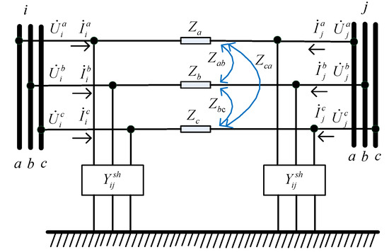
Figure 1.
Three-Phase Line Model.
The phase injection current at any bus can be expressed as the product of the bus voltage and the admittance between the buses as follows:
where n is the number of the AC bus; ; m is the phase mark, indicating three phases; and j is the phase voltage amplitude of the bus bar.
The expression for the phase power injection of the bus bar is as follows:
The phase injection current of the bus in Formula (2) is substituted into Formula (3), and the power expression can be expanded as follows:
where is the voltage phase angle difference: .
The LTC includes two parts: the “transformer” and “tap changer”. Unlike traditional transformers, an OLTC sets the tap position as an unknown variable during modelling. By controlling the amplitude of the secondary side voltage to meet a certain dead band range, the OLTC adjusts the tap position to maintain the voltage level at the load center within a certain error range, thereby enhancing the power quality for the user. This paper proposes a droop control model for the OLTC, in which the amplitude of the secondary side voltage and the tap turn ratio of the OLTC align with the droop control curve.
Defining the column name of the nodal association matrix to represent the nodes ,, , , , and , the line names correspond to the branch connected to , the branch connected to , the branch connected to , the branch connected to , the branch connected to , and the branch connected to , where , represent the nodes and , , represent the three phases of each node. The nodal correlation matrix is as follows:
According to the real and imaginary parts, the phase node power expression of the bus bar of the formula is expanded (4):
In the formula, A represents the active and reactive power of the bus and phase injection.
Among them, the active and reactive power of the branch can be expressed as follows:
3.2. Flexible Interconnection Model
The Flexible Interconnection Model consists of two or more VSC transducers connected to the DC side. When one of the transducers is out of operation due to a fault, the other transducers can continue to maintain the normal operation of the interconnection system, making the system more reliable. Figure 2 uses one end of a VSC station as an example to show the basic structure of the AC connection of a flexible interconnection device to a distribution network.
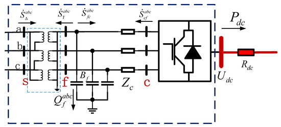
Figure 2.
VSC station structure.
In the figure, the converter station model consists of an AC bus, coupling transformer, AC filter, phase reactor, AC-DC converter, DC bus, and DC line. The AC filter is connected with the phase reactor to form a low-pass filter to prevent harmonics from entering the AC system. The MILP bad data identification method is not affected by the leverage point and can quickly and accurately identify the bad data in the leverage measurement.
3.2.1. VSC Model
In the optimization of scheduling, the voltage source converter (VSC) can be modeled as a “virtual controllable voltage source” after the phase reactor, AC filter, and transformer processing, which can be treated by the symmetric component method. The three-phase voltage and current are converted into positive-sequence, negative-sequence, and zero-sequence components and then controlled, according to specific references [22] (Ju et al., 2021). The three-phase symmetrical control mode can also be adapted to meet the negative-sequence and zero-sequence control; that is, the VSC AC side bus control is three-phase symmetric:
Transformers in converter stations usually adopt the Delta-Y three-phase transformer model as shown in Figure 3.
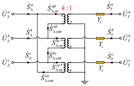
Figure 3.
Delta-Y three-phase transformer model.
The Delta-Y three-phase transformer has a triangular connection on the primary side and a star connection on the secondary side. The primary side branch power , , , , , and can be expressed as follows:
where , , and , respectively, represent the primary side bus voltage, , , , and , respectively, represent the secondary side bus voltage; is equivalent to the internal impedance of the transformer to the secondary side; and represents the ratio between the primary side and the secondary side of the transformer in the converter station.
The primary side branch power meets the constraints, as shown below:
The secondary side branch power , can be expressed as follows:
Assuming that the AC filter in the converter station has no loss, the reactive power it provides to the network is as follows:
The power flowing into the AC network at the converter bus end can be expressed as follows:
The power flowing into the phase reactor from the secondary side of the transformer can be expressed as follows:
In Formulas (12–14), is the phase scale, indicating three phases ; represents the phase voltage amplitude of the secondary side of the coupling transformer, which is equivalent to that in Figure 3 ; represents the phase voltage amplitude on the AC side of the converter; is the AC filter phase susceptance if the AC filter is not considered; and ; is the admittance of the phase reactor.
A voltage source converter can realize independent active and reactive power control, which can control the bus voltage or active power on the DC side and can also control the bus voltage or reactive power on the AC side.
For active power control, the DC part of the control includes the following two categories:
(1) Constant P control mode: the total active power injected into the AC power grid by the voltage source converter is constant, where ;
(2) Constant AC-U control mode: the converter keeps the AC bus voltage constant by adjusting the reactive power injected into the AC grid.
Due to the loss of the VSC DC transmission system to be considered, the injection of active power of the constant converter is unknown. The converter loss can be expressed using the generalized loss formula as follows:
where is the phase scale; indicate the three phases; and are the three parts of the loss coefficient: no-load loss, linear loss, and nonlinear loss of the current amplitude on the AC side of the converter.
The current amplitude of the converter is expressed as follows:
When considering the converter loss, the converter power constraint can be expressed as follows:
where the active power of the converter is injected into the DC bus . For the converter loss, is the total active power flowing into the AC network at the converter end .
According to the literature [20], when the converter station is applied to the optimal scheduling of the distribution network group, the loss of the VSC is small, so the model built in this paper ignores the impact of this loss, and the formula is simplified as follows:
3.2.2. DC Grid Model
The current injected into the DC bus is equal to the current flowing to the other buses in the DC network, expressed as follows:
where the line admittance between the DC bus and the line impedance is expressed as ; and and , respectively, are the bus voltage of the DC bus and .
The active power injected by the DC bus is as follows:
where indicates the progression of the DC system.
3.3. Data–Physics-Fusion-Driven Linearization Model
3.3.1. Physical Linearization
First, we introduce the principle of linearization based on physical properties. According to the State Grid Company’s “Grid voltage quality Technical Specifications” (Q/GDW 114-2017) [23], the voltage qualification rate of the distribution network is the ratio of the voltage qualification time of the distribution network in a certain time and the total time, which is generally stipulated to be more than 95%.
It can be considered that under the normal operation of the distribution network, the voltage amplitude of each node of the power grid is close to the rated voltage. Based on this, the approximate principle for defining the voltage amplitude of the node is as follows:
where represents the phase sequence; and represents the per unit value.
There are a large number of nonlinear sine and cosine terms in the AC power flow system, which have a great influence on the solving efficiency and convergence. In this paper, the following methods are used to deal with sine and cosine terms in trigonometric functions:
where represents the phase angle difference between the node and the node ; and represents the initial value of the phase angle difference under the normal operation state of the distribution network .
In combination with (13) and (14), the linearization of the four types of nonlinear terms in the power flow equation is carried out as follows:
For the nonlinear terms’ expressions in the converter station model, the first-order Taylor expansion is used to carry out physical linearization.
Define a function to represent the constraints of this class:
Perform a first-order Taylor expansion of the above formula:
where the formula represents the first partial derivative of the function at its initial value .
The expressions of branch power and node injection power after the linearization based on physical characteristics can be obtained by substituting the formula as (23), (27) − (28).
3.3.2. Data-Driven Error Compensation
When the end load of the distribution network is large, that is, when the line is heavy, the voltage loss on the distribution network line is large, and the voltage amplitude of the end node will be greatly offset from the rated voltage. The traditional linearization method based on physical characteristics has large errors and certain limitations. Therefore, in this paper, based on the linearization of physical characteristics, we superposition the compensation error based on the data drive, modify the linearization power equation of the power flow, and obtain the linearization expression after the data–physical fusion drive.
The compensation error expression is defined as follows:
where represents the nonlinear constraint compensation error in the node active power, reactive power balance equation, and converter station model obtained based on the data drive; is the fitting coefficient matrix and is the constant matrix, both obtained by a partial least squares regression (PLSR) analysis and fitting; is the independent variable matrix composed of the load ; and represents the vector composed of the active and reactive loads of the system’s a, b, and c phases, respectively.
(1) Data acquisition and preprocessing
First, it is necessary to collect grid operation data, including key parameters such as the node voltage, active/reactive power, and load current. The original data are cleaned (such as by eliminating outliers and filling in missing values) and standardized (such as via Z-score normalization) to ensure data quality. Subsequently, the independent variable matrix (including the three-phase loads Pa, Pb, Pc, Qa, Qb, Qc, etc.) and the dependent variable matrix (such as the residual error of the nonlinear power flow equation) are constructed to provide structured input for subsequent modeling.
(2) Error modeling based on PLSR
The data-driven error is analyzed by a partial least squares regression (PLSR), and the linear expression of the compensation error is established. The specific steps include the following (Figure 4): a PLSR is used to reduce the dimensions and regression analysis of the independent variable and dependent variable matrix, extracting the principal components to eliminate multicollinearity; the coefficient matrix and constant matrix are obtained by fitting W and C; and the compensation error model is formed . Finally, the goodness of fit of the model (such as R2, the mean square error) is verified, and the number of principal components is optimized to improve the accuracy.
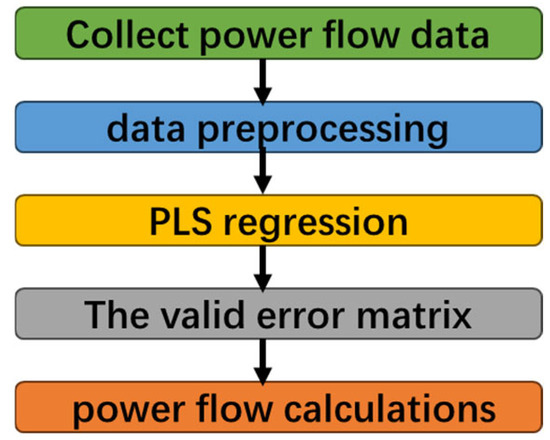
Figure 4.
The specific implementation steps of PLS.
(3) Linearization correction of physical–data fusion
The data-driven error compensation is added to the physical linearization model to correct the traditional power flow equation. After establishing the initial linearization equation based on the physical characteristics (such as the first-order Taylor expansion), the PLSR is introduced to compensate for the error. The modified power balance equation is ‘physical linearization equation + Δ’.
(4) Model validation and iterative optimization
The accuracy of the fusion model is verified by simulations or measured data. In the heavy-load scenario (such as that with a severe terminal voltage drop), the voltage estimation errors of the traditional method and the fusion model are compared, and the error distribution characteristics are analyzed. We adjust PLSR parameters (e.g., the number of principal components) or introduce dynamic update mechanisms (e.g., online learning) based on the results. If further optimization is needed, the compensation error model can be refined in combination with other data-driven methods (such as neural networks) until the engineering accuracy requirements are met.
4. Case Study
4.1. Case Study Introduction
In order to analyze and verify the effectiveness and applicability of the proposed power flow calculation method, this paper selects the 44-node system in the actual project of a province in China and the IEEE 33-bus system, as shown in Figure 5, to construct different system models.
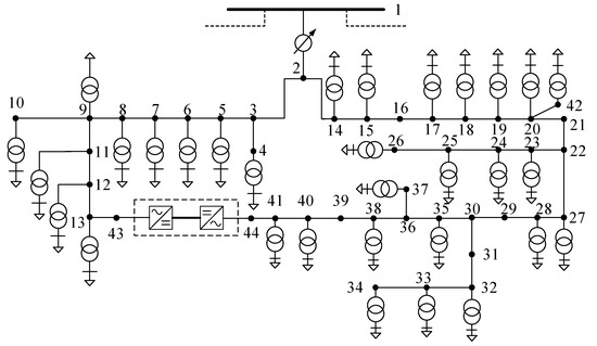
Figure 5.
Schematic diagram of the 44-node test system.
Model 1: 44-node test system of the actual project;
Model 2: 44-node test system with flexible interconnection device;
Model 3: The actual project IEEE 33-bus system;
Model 4: IEEE 33-bus system with flexible interconnection device.
4.2. Evaluation Metrics
The accuracy of the linearized models was compared by the average absolute error (AAE) and max absolute error (MAE) of the branch power in all test examples. The expressions of the AAE and MAE are as follows:
where N is the number of variables in all test examples; is the true value of the fourth variable; and is the linear value of the fourth variable calculated using the linear power flow model.
4.3. Comparison of Linearization Accuracy Under Different Scenarios
In the actual distribution system, the load of the system during the year will change with the season, weather, market, and other factors. As shown in the Figure 6 below, for different load levels, if the same data-driven error compensation model is adopted, the training samples need to include all load samples at different load levels. In this case, the load fluctuation range of the samples is large (interval A), which is not conducive to the improvement of the data-driven model’s accuracy. In this paper, a data–physical-fusion-driven linearization method is proposed to adapt to different load levels. That is, for different load levels, historical data of corresponding periods are selected to construct training samples, so as to reduce the load fluctuation range (interval a) in the sample dataset, and thus improve the data-driven error compensation accuracy.
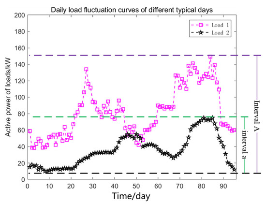
Figure 6.
Daily load fluctuation curves of different typical days.
The 42-node three-phase distribution network system in Section 4.1 is also tested. The following four test groups are set based on different seasons. In this paper, according to the simulation results and the actual situation, the scaling factor is changed to the form of the interval, and one factor in the interval can be randomly selected for the calculation. The details are as follows:
Typical scenario 1: The temperature in spring is relatively mild, and the load is generally at a medium level, which is generally lower than that in summer and winter. Therefore, the spring load is set as the reference load in this paper;
Typical scenario 2: Summer is the season with a high power load, and the use of air conditioning is high, resulting in the peak load. The summer load sample set is constructed, and the sample load is equal to the spring load multiplied by the coefficient of 120–140%;
Typical scenario 3: The temperature gradually decreases in autumn, and the load will generally decrease, but not as obviously as in spring. Therefore, the autumn load sample set is constructed, and the sample load is equal to the spring load multiplied by the coefficient of 75–80%;
Typical Scenario 4: In winter, the temperature is low, the heating load will increase, and the load in winter is usually slightly higher than that in spring. But not as summer. Therefore, the autumn load sample set is constructed, and the sample load is equal to the spring load multiplied by the coefficient of 115–125%.
The nonlinear power flow model and the linearized power flow model are used to calculate and compare the accuracy of linearization. First, the nonlinear power flow model generates data-driven training samples, in which the sample load is calculated by multiplying the rated load by a random coefficient within a specified variation range. A total of 150 training samples are used for this process.
M1: A linear power flow model driven by data–physics fusion is proposed in this paper;
M2: A linear power flow model based on Adam-DSGD proposed in the literature [15] (Liu et al., 2023);
M3: The optimal power flow of a distribution network based on the IDL model and the nonlinear adaptive data-driven model in the literature [20] (Zhang et al., 2024);
M4: A parameterized linear power flow model proposed in reference [21] (Markovic et al., 2023).
From Table 2 and Table 3, it can be seen that the three-phase power flow linearization method proposed in this paper performs best in terms of AAE and MAE values and can still maintain a high solution accuracy in different typical scenarios, reflecting the good applicability of the model under different load levels. In addition, the simulation results of the IEEE 33-bus system are equivalent to those of the 44-node system, which proves that the model has good adaptability to topology changes.
Table 2.
Comparison of AAE values.
Table 3.
Comparison of MAE values.
4.4. Analysis of Bad Data Identification Results
To verify the stability and reliability of the model proposed in this paper, the impact of different training sample sizes on the linearization accuracy is tested, which makes selecting the appropriate training sample size according to the actual situation convenient. Taking the 44-node system without a flexible interconnection device as an example, the number of training samples is further set to 120 groups, 90 groups, and 30 groups. The load level is the rated load of the system, and the random variation range of the load is 95~105% of the rated load. The AAE and MAE of the branch power obtained with different training data sample numbers are shown in the table below.
As can be seen from Table 4, the linearization method proposed in this paper can obtain a linearization error model with a high accuracy even when the number of retraining samples is small.
Table 4.
Comparison of AAE and MAE for different training data sample sizes.
4.5. Comparative Analysis of the Converter
The converter models in references [4,5,6,7] are compared in a 44-node flexible interconnected system. The comparison results are as follows Table 5:
Table 5.
Comparative analysis of the converter.
The voltage error of the model (0.35%) in this paper is 87% lower than that of Model A (2.71%) and 73% lower than Model C (1.32%). The calculation time of the model in this paper (0.95 s) is 89% higher than that of Model B (8.45 s) and better than Model C (1.78 s). The power regulation delay of the model in this paper (85 ms) is close to the SOP hardware limit (80 ms), which verifies the optimization effect of the VSC dynamic control strategy in reference [7].
4.6. Analysis of Power Flow Calculation Efficiency of Different Models
The model proposed in this paper is compared with the power flow calculation solution time of the existing data–physical fusion drive model, namely, M2, M3, and M4. The results are shown in Figure 7 The number of training samples is set to 150 groups, and the load level is selected as the typical daily load of the four seasons in one year. The example test is carried out on the MATLAB 2020 software platform. The computer processor used is an Intel (R) Core (TM) i7-8565U CPU @ 1.80GHz 1.99GHz.
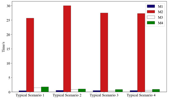
Figure 7.
Comparison of computing time.
4.7. Comparative Analysis of Initial Value Verification
To verify the effect of the traditional Newton–Raphson algorithm and the plug-and-play optimization architecture method constructed in this paper on the initial value selection strategy, the following initial value generation method is selected for analysis:
Scheme I: Predictive value based on linearized power flow;
Scheme II: Physically driven flat start (the voltage amplitude = 1 p.u. and phase angle = 0°)
The evaluation indicators are as follows:
It can be seen from Figure 7 that M1 greatly improves the time of the power flow calculation. And the other models proposed in this paper have less time to find a solution than the existing data–data-data-diiiata-data-physical-fusion-driven model.
In the formula, is the true solution of the system, is the initial guess of the algorithm, is the solution at the end of the iteration of the algorithm, and is the error transfer rate.
As shown in Table 6, the data show that under the same initial value strategy, the proposed method significantly reduces the sensitivity to the initial error (the error transfer rate is reduced by 84.6%), which indirectly verifies the improvement of the robustness of the initial value.
Table 6.
Comparative analysis of initial value verification.
5. Conclusions
Because the traditional power flow calculation method cannot meet the calculation accuracy of the new power system, the data-driven power flow calculation needs to meet the requirements of a large number of datasets and cannot retain the physical characteristics of the system. In order to adapt to the calculation accuracy and calculation efficiency of the current flexible interconnected distribution network power flow, this paper draws the following two conclusions:
(1) This paper considers the characteristics of electronic power components of a VSC introduced by distributed power generation and establishes a power flow calculation model suitable for the current flexible interconnected distribution network;
(2) An LPFC model driven by data–physical fusion is proposed. The physical model combined with a partial least squares regression (PLSR) is used to compensate for the error of the nonlinear term, which not only improves the solution efficiency, but also significantly improves the accuracy of the power flow calculation. The feasibility and effectiveness of the proposed data–physical-fusion-driven LPFC method are verified by an actual 44-bus system and a power system with flexible interconnection devices.
Author Contributions
W.L., Y.Y. and T.L. contributed to the conceptualization, methodology, software development, validation, formal analysis, investigation, data curation, and writing of the original draft. Y.J. and Y.M. contributed to the supervision, project administration, review, and editing, as well as the funding acquisition. All authors have read and agreed to the published version of the manuscript.
Funding
This paper is sponsored by Science and Technology Project of State Grid Liaoning Electric Power Supply Co., Ltd. (project name: Research on Planning and Design Technology of Active Distribution Network Sensing System for Large-scale Access of Distributed Power Sources; project number: 2024YF-29).
Data Availability Statement
The original contributions presented in this study are included in the article. Further inquiries can be directed to the corresponding authors.
Acknowledgments
The authors express their gratitude to the editors and reviewers for their valuable feedback and support in advancing this work.
Conflicts of Interest
Authors Wanyuan Li, Yang You and Tianze Liu were employed by the State Grid Panjin Electric Power Supply Company, State Grid Liaoning Electric Power Supply Co., Ltd. The remaining authors declare that the research was conducted in the absence of any commercial or financial relationships that could be construed as a potential conflict of interest.
References
- Wang, L.; Zhao, H.; Yu, Q.; Wen, Q.; Zhang, Y.; Wang, W. Linear Power Flow Calculation Methods for Urban Network. In Proceedings of the 2022 IEEE/IAS Industrial and Commercial Power System Asia (I&CPS Asia), Shanghai, China, 8–11 July 2022. [Google Scholar] [CrossRef]
- Yang, Z.; Xie, K.; Yu, J.; Zhong, H.; Zhang, N.; Xia, Q. A General Formulation of Linear Power Flow Models: Basic Theory and Error Analysis. IEEE Trans. Power Syst. 2019, 34, 1315–1324. [Google Scholar] [CrossRef]
- Yang, J.; Zhang, N.; Kang, C.; Xia, Q. A State-Independent Linear Power Flow Model with Accurate Estimation of Voltage Magnitude. IEEE Trans. Power Syst. 2017, 32, 3607–3617. [Google Scholar] [CrossRef]
- Wei, Z.; Zhang, Q.; Zhao, J.; Liu, J.; He, T.; Sun, G.; Zang, H. Review and Improvement of Power System Linearization Models. Power Syst. Technol. 2017, 41, 2919–2927. [Google Scholar] [CrossRef]
- Yin, S. Research on Modeling and Application of Converter Operating State Based on Port Current Timing Characteristics; South China University of Technology: Guangzhou, China, 2022. [Google Scholar] [CrossRef]
- Liang, G.; Zhang, J. Research on modulation strategy of modular multilevel converter. Electr. Technol. 2021, 5, 15–18+23. [Google Scholar] [CrossRef]
- Lian, P.; Liu, W.; Tang, Y.; Yang, Z.; Yu, S.; Li, X. Research on efficient electromagnetic transient simulation method of modular multilevel converter. Chin. J. Electr. Eng. 2020, 40, 7980–7989+8235. [Google Scholar] [CrossRef]
- Fan, Z.; Yang, Z.; Yu, J. Error Bound Restriction of Linear Power Flow Model. IEEE Trans. Power Syst. 2022, 5, 808–811. [Google Scholar] [CrossRef]
- Garces, A. A Linear Three-Phase Load Flow for Power Distribution Systems. IEEE Trans. Power Syst. 2016, 31, 827–828. [Google Scholar] [CrossRef]
- Yuan, Z. Formulations and Approximations of Branch Flow Model for General Power Networks. J. Mod. Power Syst. Clean Energy 2022, 10, 1110–1126. [Google Scholar] [CrossRef]
- Chen, J.; Wu, W.; Roald, L.A. Data-Driven Piecewise Linearization for Distribution Three-Phase Stochastic Power Flow. IEEE Trans. Smart Grid 2022, 13, 1035–1048. [Google Scholar] [CrossRef]
- Liu, Y.; Zhang, N.; Wang, Y.; Yang, J.; Kang, C. Data-Driven Power Flow Linearization: A Regression Approach. IEEE Trans. Smart Grid 2019, 10, 2569–2580. [Google Scholar] [CrossRef]
- Li, P.; Wu, W.; Wang, X.; Xu, B. A Data-Driven Linear Optimal Power Flow Model for Distribution Networks. IEEE Trans. Power Syst. 2023, 38, 956–959. [Google Scholar] [CrossRef]
- Liu, Y.; Li, Z.; Sun, S. A Data-Driven Method for Online Constructing Linear Power Flow Model. IEEE Trans. Ind. Appl. 2023, 59, 5411–5419. [Google Scholar] [CrossRef]
- Shao, Z.; Zhai, Q.; Wu, J.; Guan, X. Data-Based Linear Power Flow Model: Investigation of a Least-Squares Based Approximation. IEEE Trans. Power Syst. 2021, 36, 4246–4258. [Google Scholar] [CrossRef]
- Tan, Y.; Chen, Y.; Li, Y.; Cao, Y. Linearizing Power Flow Model: A Hybrid Physical Model-Driven and Data-Driven Approach. IEEE Trans. Power Syst. 2020, 35, 2475–2478. [Google Scholar] [CrossRef]
- Ju, Y.; Yang, M.; Wu, W. Hybrid Data-Physical-Driven Linearization Method for Three-Phase Optimal Power Flow in Distribution Network. Autom. Electr. Power Syst. 2022, 46, 43–52. [Google Scholar] [CrossRef]
- Bazrafshan, M.; Gatsis, N. Comprehensive Modeling of Three-Phase Distribution Systems via the Bus Admittance Matrix. IEEE Trans. Power Syst. 2018, 33, 2015–2029. [Google Scholar] [CrossRef]
- Shao, Z.; Zhai, Q.; Guan, X. Physical-Model-Aided Data-Driven Linear Power Flow Model: An Approach to Address Missing Training Data. IEEE Trans. Power Syst. 2023, 38, 2970–2973. [Google Scholar] [CrossRef]
- Zhang, Y.; Guo, L.; Liu, Y.; Wang, Z.; Li, X.; Bai, L.; Wang, C. Nonlinearity-Adaptive Data-Driven Power Flow Constraint for Distribution Network Optimization. IEEE Trans. Power Syst. 2024, 39, 341–354. [Google Scholar] [CrossRef]
- Markovic, M.; Hodge, B.-M. Parameterized Linear Power Flow for High Fidelity Voltage Solutions in Distribution Systems. IEEE Trans. Power Syst. 2023, 38, 4391–4403. [Google Scholar] [CrossRef]
- Ju, Y.; Liu, W.; Wang, J.; Li, J.; Huang, Y.; Chen, X.; Dong, Z. Power Flow Analysis of Integrated Energy Microgrid Considering Non-Smooth Characteristics. IET Gener. Transm. Distrib. 2021, 16, 2777–2790. [Google Scholar] [CrossRef]
- Q/GDW 114-2017; Grid Voltage Quality Technical Specifications. State Grid Corporation of China: Beijing, China, 2017.
Disclaimer/Publisher’s Note: The statements, opinions and data contained in all publications are solely those of the individual author(s) and contributor(s) and not of MDPI and/or the editor(s). MDPI and/or the editor(s) disclaim responsibility for any injury to people or property resulting from any ideas, methods, instructions or products referred to in the content. |
© 2025 by the authors. Licensee MDPI, Basel, Switzerland. This article is an open access article distributed under the terms and conditions of the Creative Commons Attribution (CC BY) license (https://creativecommons.org/licenses/by/4.0/).