Comparison Between AICV, ICD, and Liner Completions in the Displacement Front and Production Efficiency in Heavy Oil Horizontal Wells

Abstract

Autonomous inflow control devices (AICDs) offer a promising means of delaying early water breakthrough in heavy oil horizontal wells; yet, current design practices remain largely empirical. A three-dimensional, field-calibrated computational fluid dynamics (CFD) model was developed to establish a mechanistic basis that solves the transient Navier–Stokes equations for turbulent two-phase flow via a volume-of-fluid formulation. Pressure-controlled inflow boundaries were tuned to build up data from four Colombian heavy oil producers, enabling a quantitative comparison with production logs. Model predictions deviate by no more than ±14% for oil rate and ±10% for water rate over a 500-day horizon, providing confidence in subsequent scenario analysis. Replacing a slotted liner completion with optimally sized AICDs lowers cumulative water-cut by up to 93%, reduces annular friction losses by 18%, and cuts estimated life cycle CO₂ emissions per stock-tank barrel by 82%. Sensitivity analysis identifies nozzle diameter as the dominant design variable, with a nonlinear interaction between local drawdown pressure and the oil–water viscosity ratio. These findings demonstrate that CFD-guided AICD design can materially extend wells’ economic life while delivering substantial environmental benefits. The validated workflow establishes a low-risk, physics-based path for tailoring AICDs to reservoir conditions before field deployment.

1. Introduction

Advancements in technology have ushered in a new era where society can enhance production efficiency while mitigating the environmental impact and reducing industrial costs. Amidst the ongoing energy transition, a pivotal focus for oil producers lies in augmenting oil production efficiency to facilitate a smoother transition. However, heavy oil producers encounter a formidable obstacle, notably excessive water production. Associated water production often surpasses oil production by up to fiftyfold, resulting in a steep escalation of lifting costs, energy expenditure, carbon emissions, and a decrease in the recovery factor, particularly at water-cuts exceeding 90% [1,2,3]. Addressing this challenge, various innovative technologies have emerged, such as Downhole Water Mechanical Devices, encompassing different iterations such as inflow control devices (ICDs), inflow control valves (ICVs), autonomous control devices (AICDs), and autonomous control valves (AICVs). These are examples of Intelligent Completion Technologies, which entail the installation of static or autonomous devices along the completion of a horizontal well to regulate fluid inflow, uniformizing the drawdown. The primary objective is to ensure uniform fluid inflow within the well horizontal section, with less water production, thereby enhancing oil production efficiency and curbing water production [4,5]. These innovative water-management technologies enable more sustainable oil production by reducing environmental impacts while maximizing resource recovery in mature heavy oil fields. This approach supports UN Sustainable Development Goals 7 (Affordable and Clean Energy), 9 (Industry, Innovation and Infrastructure), and 13 (Climate Action) through minimized carbon footprints, enhanced energy efficiency, and responsible resource utilization.

The operational principles of these technologies have been elucidated by numerous researchers across a broad spectrum of designs. For instance, passive ICDs employ channels and orifices to manage pressure drop and fluid inflow [6,7,8,9,10,11]. Conversely, more sophisticated variants like AICDs, with or without moving components, are utilized to control flow. Examples include designs without moving parts, such as diode configurations [12,13,14,15,16,17], or those with moving components like disks and flappers, such as RCP valves, which regulate flow through the actuation of moving parts. Finally, the latest generation of AICVs boasts superior efficiency to AICDs and incorporates autonomous moving parts, like disks, capable of choking fluid inflow by up to 90% [18,19,20,21].

However, challenges in their proper implementation diminish their efficacy, with the most crucial issue being optimal design. This entails considerations such as the number of valves along the well, their positioning, dimensional aspects, and other factors [19,22,23]. Additionally, forecasting their dynamic behavior, influenced by multiphase flow in both the reservoir and the well, poses further complexity. This dynamic interplay affects displacement stability, well inflow uniformity, and pressure drop along the well.

Optimization methodologies based on the wellbore-to-reservoir pressure drop ratio have been developed [5,24], resolving well–reservoir interaction dynamics through multisegment well modeling. Unlike the full Navier–Stokes simulations employed in our study, these approaches utilize reduced-order modeling techniques. Nevertheless, they enable effective AICD completion design by predicting optimal AICD placement and quantity, device type selection, and comparison-specific AICD density.

Similarly, other researchers have conducted studies addressing optimal inflow technology and design. For instance, comparisons among various types of ICDs, AICDs, and AICVs have been explored in previous work [19,23,25,26]. Most studies have employed reservoir simulators capable of dynamically coupling the wellbore and reservoir. These studies reveal that all inflow devices delay early water breakthroughs compared to conventional liners. Moreover, AICD/AICVs demonstrate superior performance compared to passive ICDs. Variables impacting the efficacy of AICD/AICVs, such as reservoir heterogeneity, fractures, and swell packer size, have been considered in these studies.

Parallelly, rapid advancements in computational capabilities have facilitated a deeper understanding and more detailed design of Downhole Water Mechanical Devices through Computational Fluid Dynamics (CFD) studies. Conventional CFD codes typically solve the complete set of Navier–Stokes equations in 3D, coupled with closure relations, enabling more detail on the multiphase flow phenomena occurring near the wellbore and directly within the well. This advanced level of detail has been thoroughly demonstrated in recent CFD investigations [27,28,29,30,31]. Moreover, they can explicitly depict the flow dynamics between the reservoir (near wellbore) and the well down completion with or without different Water Control Devices, either static or dynamic. The flow dynamics coupling well and reservoir systems have been extensively investigated [31,32,33,34,35], focusing on reservoir heterogeneities, formation damage, annulus configurations, and performance comparisons between Water Control Devices and conventional technologies like sand screens.

Key features observed in such studies include explicit modeling of single- and multiphase flow dynamics, numerical calculations of friction and obstruction losses, turbulence effects, material erosion analysis, fluid–solid interaction, and performance curve derivation. Examples of CFD-assisted design for diode-type AICDs are documented in [14,36,37], while passive ICD and alternative AICD configurations are examined in [18,38,39,40,41,42]. Additionally, coupled CFD and fluid–solid interaction (FSI) simulations of moving-part valves (e.g., RCP types) are demonstrated in [43].

CFD technology can overcome limitations in studying the design of Downhole Water Mechanical Devices completion. For instance, it leverages the Navier–Stokes equations in 3D to provide a more detailed description of multiphase flow within the device and the well and reservoir, utilizing complete Eulerian solutions for each phase. Moreover, CFD can solve fluid flow from near the wellbore into the horizontal section and through the Downhole Water Mechanical Device (fixed or autonomous) rather than relying on coupling separate solutions and leveraging the device performance curves [4,22].

This study aims to advocate for CFD as a tool for designing Intelligent Wells and Well Management strategies to mitigate water pollution, lower energy consumption, and decrease carbon emissions during oil production. Therefore, this study presents a comparative CFD analysis of different Downhole Water Mechanical Devices—ICD, AICD, and slotted liners—for heavy oil wells in the Llano Basin, Colombia. It examines their influence on aquifer disturbance, displacement front stability, well fluid dynamics, and oil and water production profiles. A comparative analysis between these completion technologies was conducted across different wells to determine their effectiveness in improving production efficiency by substantially reducing water production. The impact on the CO₂ footprint was also estimated.

2. Methodology

The numerical models were constructed utilizing commercial CFD Software STAR-CCM+ v2402 (Siemens, Germany) previously used in other studies [31]. To elucidate the multiphase flow dynamics of heavy oil/water in the reservoir, near the wellbore, within the completion, and throughout the well, the Eulerian Volume of Fluid (VOF) model with the High-Resolution Interface Capturing scheme was implemented. Additionally, gravity was accounted for as a significant force influencing phase segregation, impacting not only the reservoir rock but also the completion and the well. The numerical code employs a segregated solver with the SIMPLE algorithm to solve the conservation equations.

Conversely, four (4) horizontal heavy oil wells were considered for this study, each with distinct completion designs and Downhole Water Mechanical technologies (ICD/AICD/slotted liner). Furthermore, reservoir heterogeneity was incorporated using data from well-logging measurements in the field. It is important to note that no manufacturer has considered the detailed geometry of fixed and autonomous devices. Instead, the effect of these devices was considered through the boundary conditions. Namely, to simulate choking in the AICD study cases, a flow restriction was programmed at the boundary between the device hole and the upstream section. Finally, it should be noted that all wells were modeled using an expandable screen configuration along the wellbore. This approach simulates a scenario in which the screen is in direct contact with the reservoir rock, disregarding the presence of any annular space or formation damage effects. All simulations were executed on a computer with an 8-core Intel Xeon E5-2690 processor and 64 GB of RAM. As a result, on average, all simulations required about a week for modeling 100 production days.

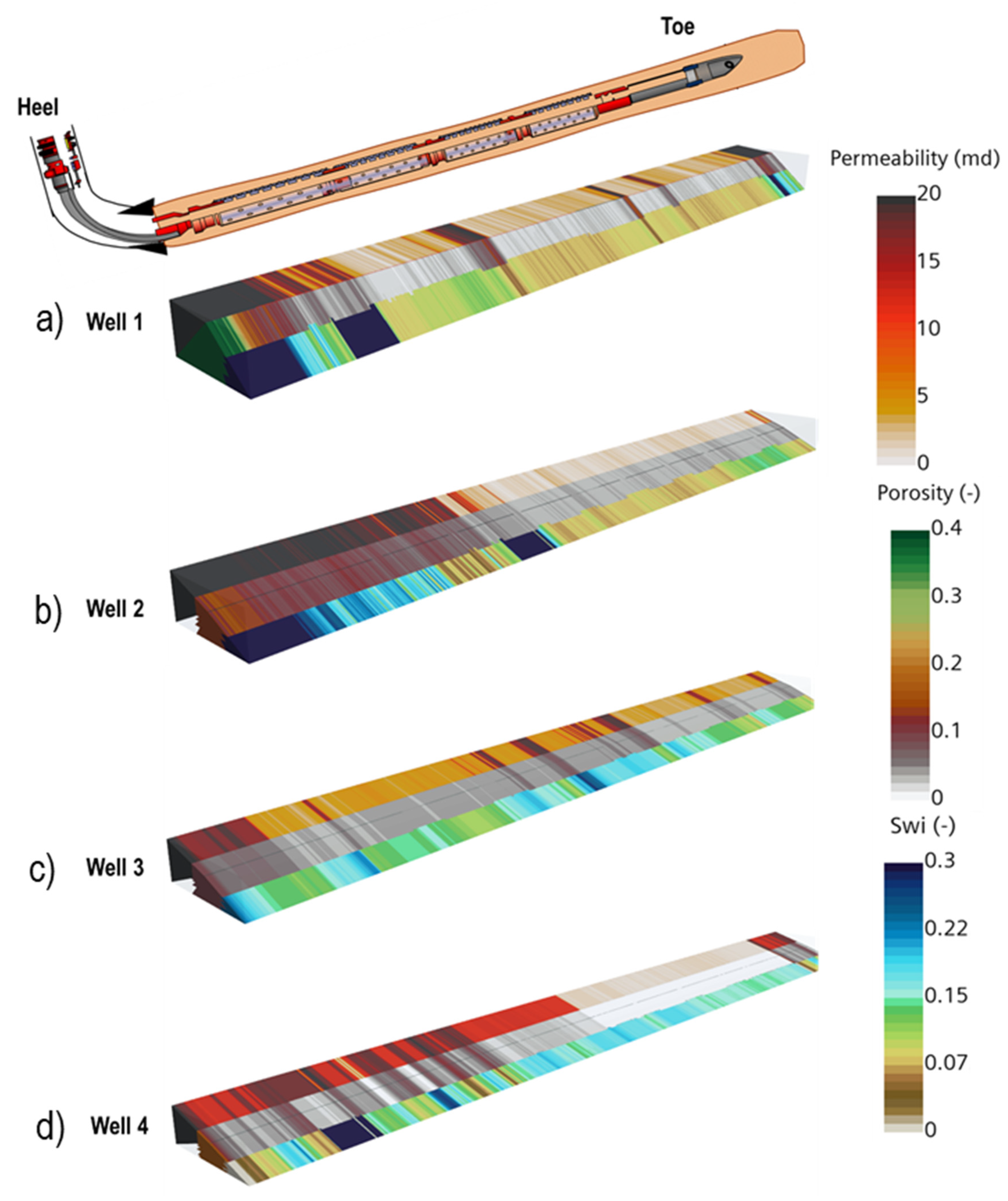
2.1. Initial and Boundary Conditions: Horizontal Completion and Reservoir Information

For this study, four distinct oil wells in the Llano Basin, Colombia, were examined. Figure 1 illustrates fundamental reservoir properties, including permeability, porosity, and initial saturation. Furthermore, reservoir heterogeneity was accounted for using data gathered from well-logging measurements at 0.5 ft intervals for each well. Conversely,

Table 1. Main information related to the reservoir and completion for each well.

Well	1	2	3	4
Reservoir Formation	Unconsolidated Sands	Unconsolidated Sands	Unconsolidated Sands	Unconsolidated Sands
Outer Annulus	Closed/Collapsed: Averaged porous properties from Figure 1 were implemented	Closed/Collapsed: Averaged porous properties from Figure 1 were implemented	Closed/Collapsed: Averaged porous properties from Figure 1 were implemented	Closed/Collapsed: Averaged porous properties from Figure 1 were implemented
Completion Simulated	Slotted Liner	$\mathrm{Autonomous} \mathrm{Devices} (8 \mathrm{D}\mathrm{e}\mathrm{v}\mathrm{i}\mathrm{c}\mathrm{e}\mathrm{s})$	$\mathrm{Autonomous} \mathrm{Devices} (8 \mathrm{D}\mathrm{e}\mathrm{v}\mathrm{i}\mathrm{c}\mathrm{e}\mathrm{s})$	Fixed Devices $(30 \mathrm{D}\mathrm{e}\mathrm{v}\mathrm{i}\mathrm{c}\mathrm{e}\mathrm{s})$
Total Number of Isolations	$0$	$8$	$8$	$8$
$\mathrm{Reservoir} \mathrm{Pressure} \left(psi\right)$	$1250$	$1312$	$1200$	$1200$
$\mathrm{Well} \mathrm{Length} \left(ft\right)$	$800$	$800$	$900$	$950$
$\mathrm{Reservoir} \mathrm{Horizontal} \mathrm{Dimension} \left(ft\right)$	$80$	$80$	$80$	$80$
$\mathrm{Reservoir} \mathrm{Vertical} \mathrm{Dimension} \left(ft\right)$	$40$	$40$	$40$	$40$
$\mathrm{Completion} \mathrm{Diameter} \left(in\right)$	$6.5/8$	$6.5/8$	$6.5/8$	$6.5/8$
$\mathrm{Oil} \mathrm{Density} \left(API\right)$	$11$	$12$	$12$	$12$
$\mathrm{Oil} \mathrm{Viscosity} \left(cp\right)$	$500$	$600$	$600$	$600$

summarizes crucial data about each well, such as completion type and fluid properties. Additionally, Figure 2 outlines primary boundary conditions and features such as screens, blank liners, annulus, and the Downhole Water Mechanical Devices.

The CFD model delineates the multiphase flow dynamics among the reservoir, completion, and well. The domain was subdivided into these main subdomains or regions to initialize and implement physical models in the studied cases. For instance, the reservoir rock subdomain was initialized with the initial water saturation and porous properties detailed in Table 1. The horizontal well completion (annulus, screens, Water Control Devices, and well) was initialized based on the average volume fraction obtained from field data, serving as a benchmark for numerical validation. Conversely, the horizontal well completion was fully initialized with oil in numerical experiments conducted under constant drawdown conditions. Across all subdomains, the pressure field was set to the reservoir pressure, while the velocity field was uniformly initialized to zero.

Similarly, screens and slotted liners were modeled as porous regions with inertial and viscous concentric flow resistances to streamline computational efficiency rather than considering individual holes and slots. Moreover, fixed devices were programmed to remain fully open, while the autonomous ones were set to choke flow by up to 95% of flow area restriction once a water-cut of 90% was reached on each device. In this study, for cases involving Water Control Devices, isolation was implemented in both the inner and outer annulus, with the latter achieved through swellable packers. In this study, the swellable packers were treated as no-flow zones. Additionally, it was assumed that all wells utilized expandable screens, simulating direct contact between the screen and the reservoir rock, disregarding the presence of an annulus, formation damage, or the effects of any mud cake between the well and the reservoir rock.

The primary boundary conditions were defined as follows: the enclosing impermeable walls were treated as wall boundary conditions. The bottom aquifer was modeled as an inlet boundary condition with a constant pressure equal to the reservoir pressure. The outlet boundary condition was set at the well outlet/heel and maintained at a constant pressure equal to the bottomhole flowing pressure. This outlet condition was configured using reported field data for history matching or at a continuous drawdown for the numerical experiments. This combination of boundary conditions ensured an accurate representation of the physical phenomena, satisfied mass conservation equations, and maintained numerical stability.

The CFD model was developed based on the following key considerations:

• Wellbore–formation interface effects (e.g., annulus/mud cake) were excluded to enable focused comparison of completion types under equivalent boundary conditions, consistent with standard simulation practice.
• Reservoir properties were maintained to isolate completion effects—a well-documented approach in controlled comparative simulation studies.
• While field-scale heterogeneities beyond our 3D simulation domain were not incorporated, their impact would affect all completion types proportionally, preserving relative performance trends.

2.2. Discretization of the Domain

The 3D models of the various wells were numerically solved using the finite volume method, a widely used technique in reservoir simulation. This method discretizes the domain into a finite number of control volumes, allowing for an accurate representation of fluid flow. Consequently, an unstructured hexahedral mesh was employed throughout the entire domain. In the reservoir rock, mesh density was heightened near the wellbore to enhance numerical stability and resolve the unstable displacement, particularly near the breakthrough event. Additionally, the mesh in the well underwent refinements near the wall to accurately capture near-wall effects and their impact on flow dynamics and pressure drop along the well, effectively capturing the Heel-to-Toe effect.

The average number of cells or control volumes for the different cases is 1,300,000, facilitating the representation of fluid flow, unstable displacement in the reservoir rock, and fluid dynamics within the well. Notably, in the fixed devices case, like ICD ones, they were programmed to never close during or after the breakthrough event. Conversely, in autonomous device cases, like ACID, after the water breakthrough, the total flow into the well is regulated to be choked up to 90–95% when the autonomous devices register a water-cut equal to or greater than 90%.

A general overview of the implemented mesh is shown in Figure 3. The average length-to-radius ratio in the horizontal wellbore section was approximately 1600. Despite this high aspect ratio, no numerical issues were encountered, thanks to enhanced mesh density in critical areas such as the ICD/AICD holes and near the inflow sections of the various completions. The details of the average number of elements used for each subdomain mesh are presented in

Table 2. Detailed information about the mesh for each subdomain.

Subdomain	Average Number of Elements
Reservoir Rock	$\mathrm{1,010,486}$
Slotted Liner/Screens	19,197
Annulus	13,438
Water Control Device	235,458
Horizontal Well	55,096

. These regions typically exhibit intense pressure and velocity gradients due to reduced flow area and the transition from porous media flow to free flow. However, the improved mesh refinement effectively mitigated potential convergence issues.

2.3. Governing Equations and Assumptions

The conservation equations for mass, momentum, and energy govern the CFD model. The k-ω SST turbulence model, a popular choice for simulating turbulent flows, was also implemented to account for the free-flow conditions in the completion and wellbore regions. This model provides a good balance between accuracy and computational cost. Due to the complexity of the problem, the following simplifications were applied:

• Newtonian flow: The system’s rheology was assumed to be Newtonian and constant over time, excluding any non-Newtonian behavior that could arise from the emulsified flow.
• Outer annulus: The outer annulus of the completions, defined as the space outside the sand screen, was modeled as an uncollapsed hole, meaning that the wells were modeled as expandable sand screens. This region was simulated as a porous flow zone using the heterogeneous reservoir porous properties previously depicted in Figure 1, without considering it a gravel packing zone or any other phenomena such as formation damage or mud cakes.

Equation (1) gives the continuity equation, representing the conservation of mass. This equation ensures that mass is conserved in the system. Similarly, the linear momentum equation, described by Equation (2), ensures that momentum is conserved in the system.

$${\displaystyle \frac{\partial \rho }{\partial t}}+\nabla ·\left(\rho v\right)=0$$

(1)

where $\rho$ is the density and $v$ is the velocity.

The linear momentum equation is described by Equation (2):

$${\displaystyle \frac{\partial \left(\rho v\right)}{\partial t}}+\nabla ·\left(\rho v\otimes v\right)=\nabla ·\sigma +f_b+S_t$$

(2)

where $f_b$ represents external forces acting on the system, $\sigma$ is the stress tensor, and $S_t$ is a momentum sink term. In this context, the momentum sink corresponds to the porous media flow model, as described by Equation (3):

$$S_t={\displaystyle \frac{\mu }{k}}+{\displaystyle \frac{C\rho }{2}}{v}_s$$

(3)

where $\mu$ is the fluid’s viscosity, $k$ is the permeability of the media, and $C$ is the coefficient of the inertial flow resistance factor.

3. Results

This section outlines the primary findings through two subsections. The first subsection delves into the performance of the 4 distinct wells, emphasizing the thorough analysis of the emulation of field data, albeit limited to Wells 1, 2, and 3. Well 4 data was unavailable and only numerical results are presented. The second subsection, using CFD as a Virtual Lab, presents a comparative analysis of different completions and varying inflow technologies: slotted liners and AICD for Wells 2 and 3, and slotted liners, AICD, and ICD for Well 4. All assessments are conducted under constant drawdown conditions.

3.1. Comparison of Current Field Implementations

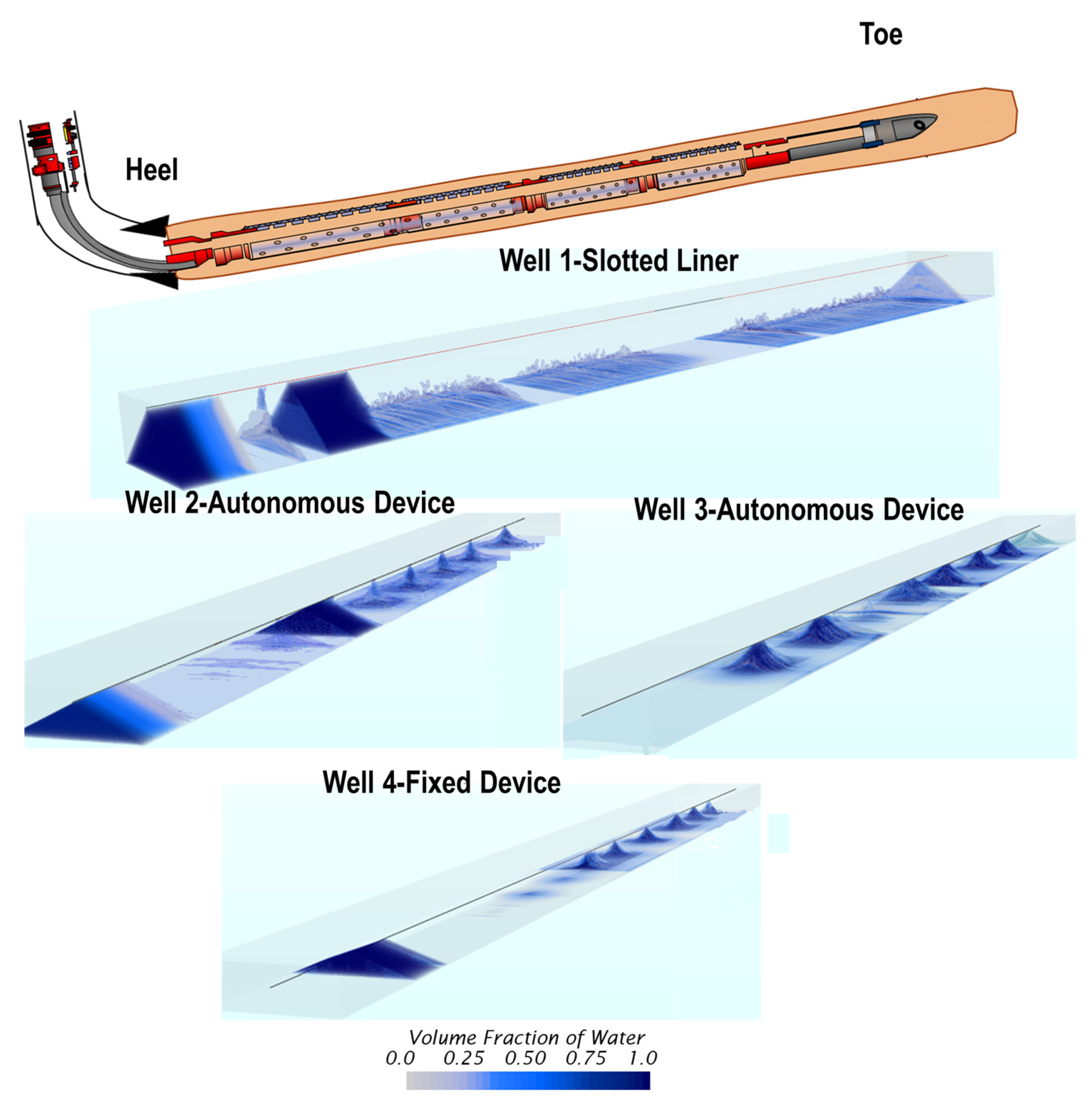
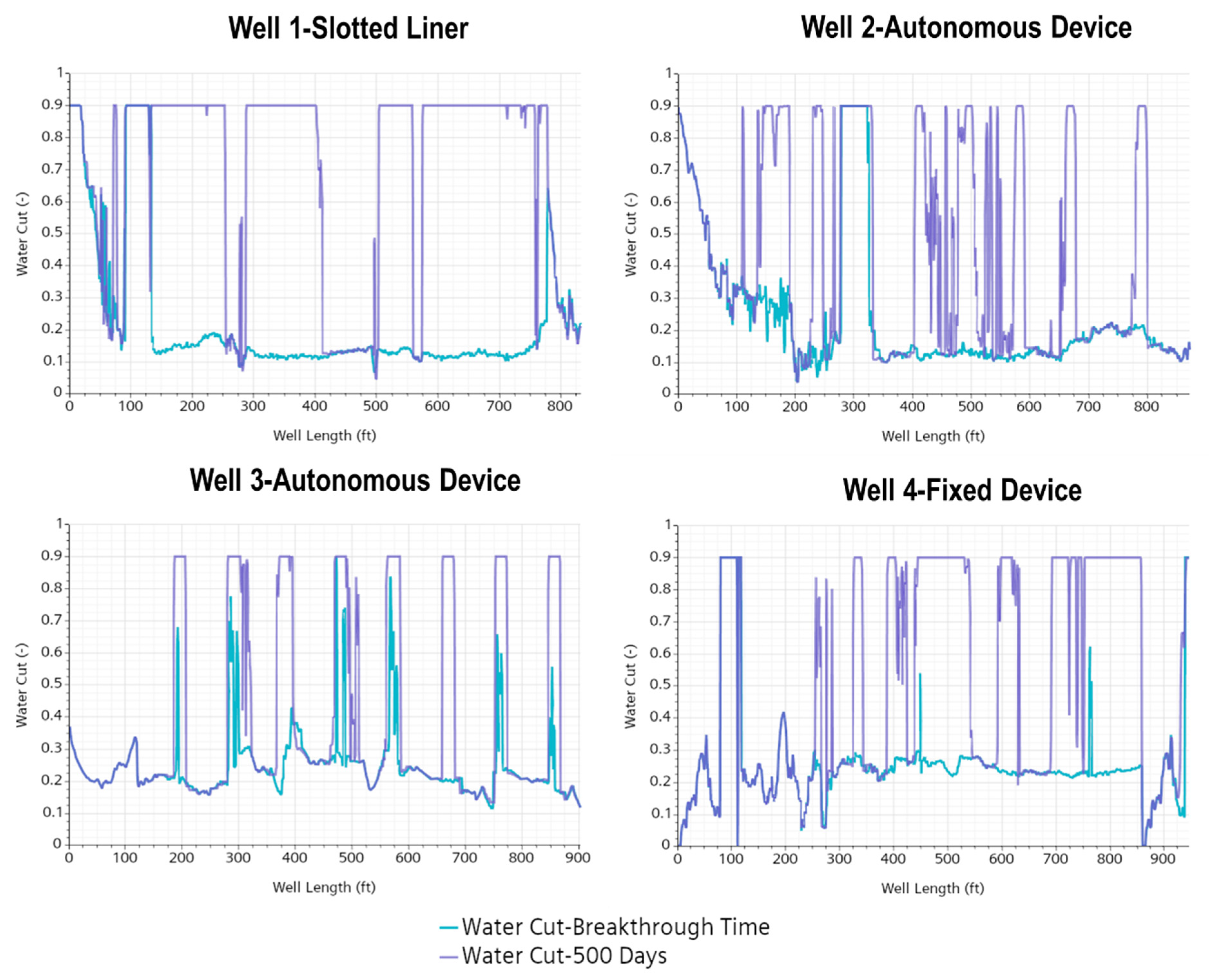
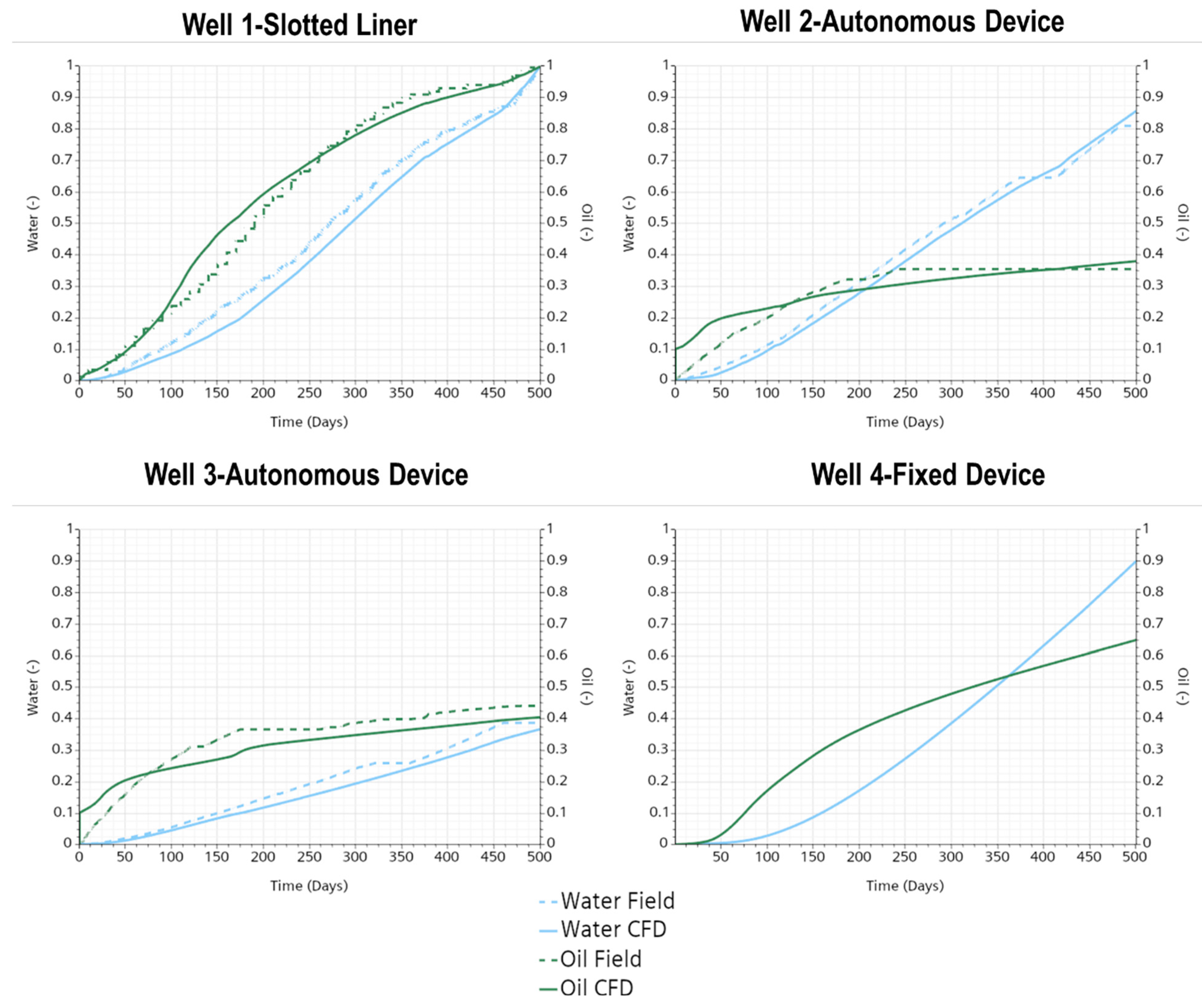
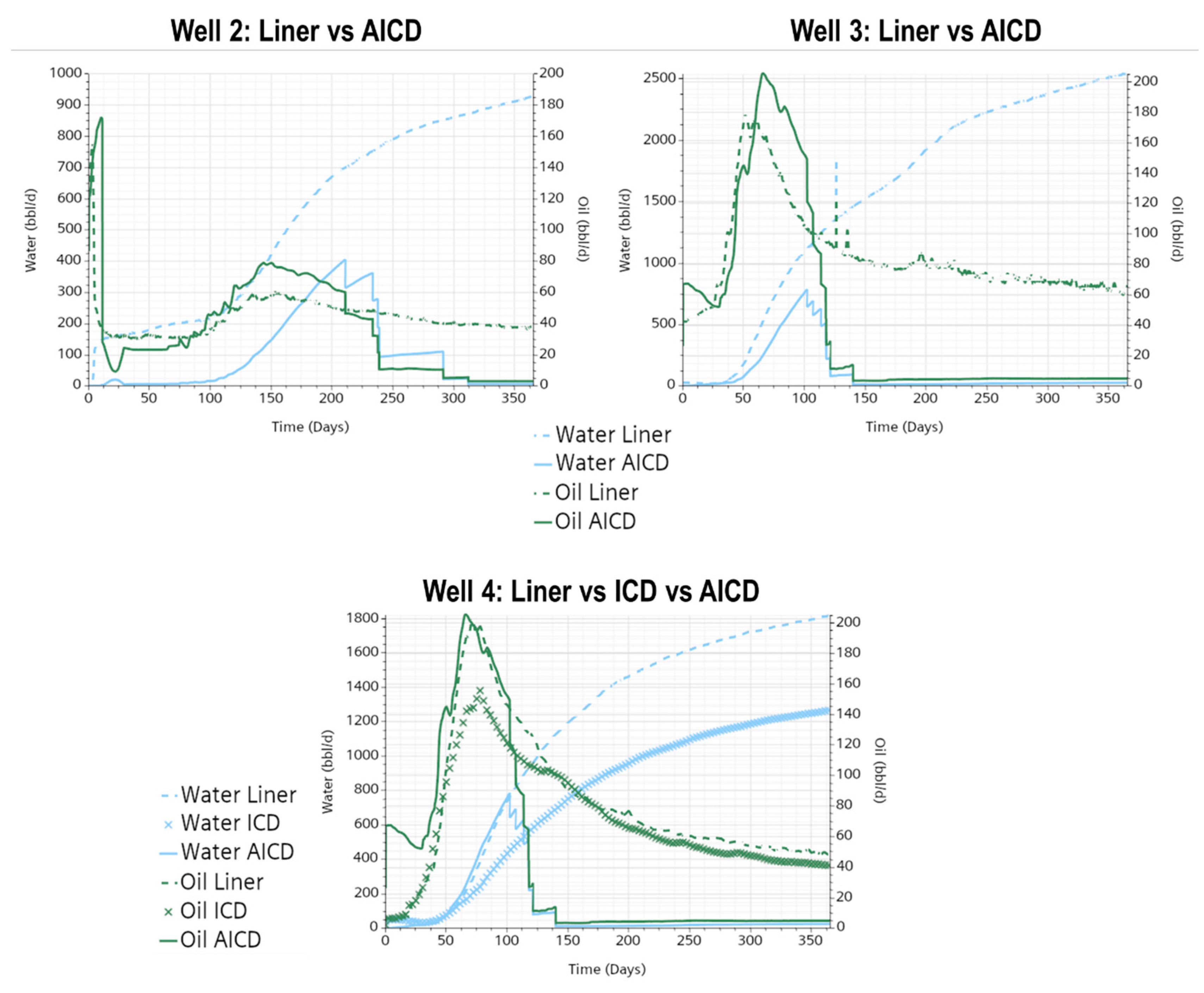
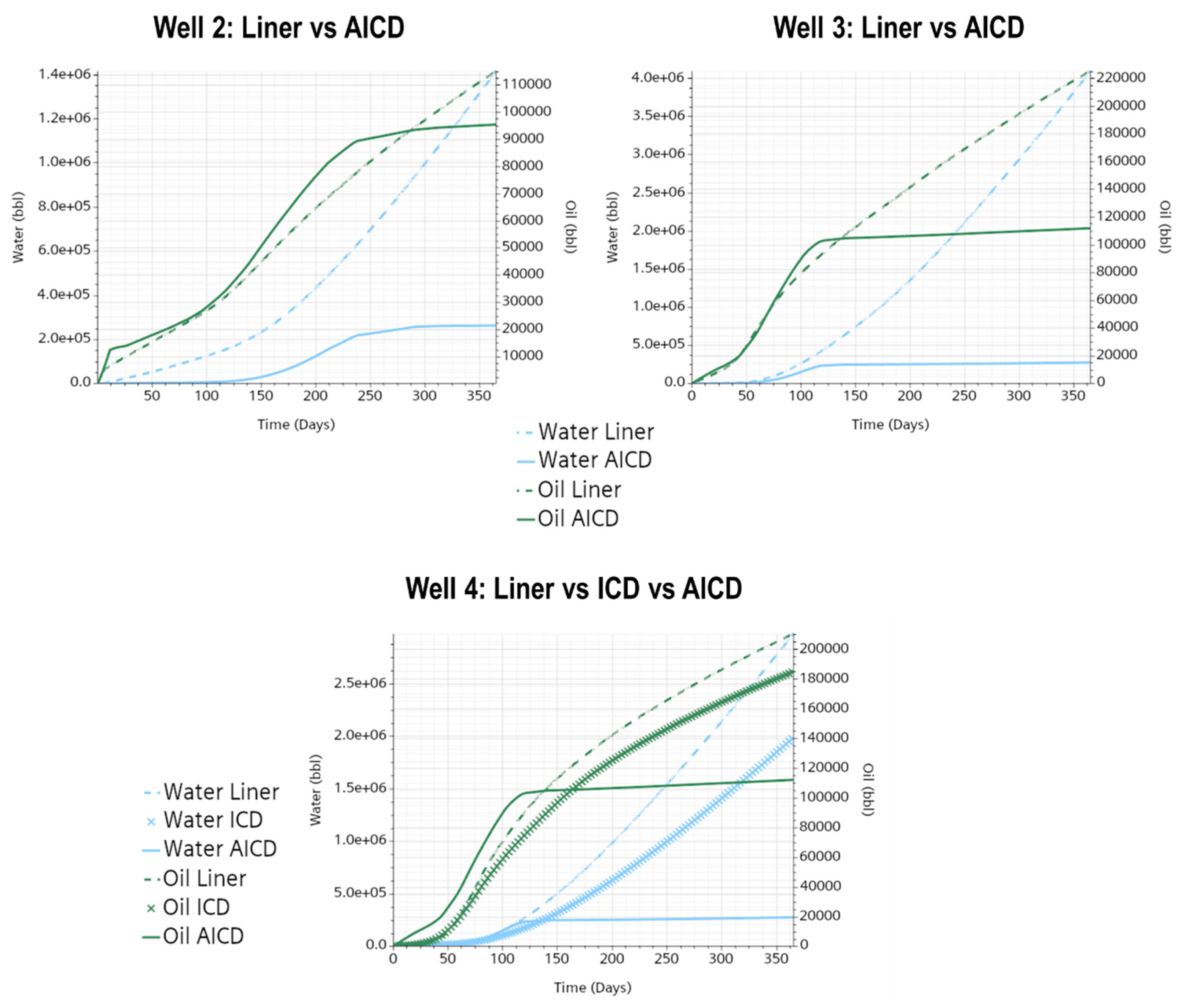
3.1.1. Reservoir Water Displacement and Production

One of the most significant contributions of the CFD models lies in their ability to provide an enhanced or detailed depiction of fluid movement within the reservoir, which goes into the well. In this instance, the models of Wells 1, 2, and 3 replicated typical production operational conditions as a reference. In contrast, Well 4 was simulated under a constant drawdown of 14 psi.

Figure 4 and Figure 5 offer a comprehensive view of water displacement under fifteen (15) months of regular operation, first showing the breakthrough event and the water movement after 500 days. These figures present 3D renderings of water movement within the reservoir, depicted as water saturation or volume fraction. To enhance the clarity of the visualization, the oil phase was omitted using post-processing techniques.

Overall, as frequently imagined and only seen under experimental conditions, all the wells studied, regardless of the inflow technology utilized, exhibited pronounced non-uniform water displacement due to the adverse oil–water mobility ratio. That means the aquifer at the bottom tended to channel along the horizontal well. Figure 4 illustrates that during the initial breakthrough, the channels were thin and well-defined below the liners in Well 1 and below the screens near the Downhole Mechanical Devices for the other wells. Additionally, the appearance of small channels from the aquifer can be depicted in Wells 1, 2, and 4.

Following traditional theories, the coning is represented in what would correspond to the heel section of each well. The area and intensity of water production are higher than the rest of the horizontal section. As expected in the case of the well employing conventional completion, Well 1, the disturbance of the aquifer at breakthrough time is particularly pronounced. Initially, small channels along the horizontal well gradually evolve into robust crests, as depicted in Figure 5. This figure illustrates the exacerbation of water channeling across all the examined wells, with wider, longer, and darker channels inundating the entire horizontal section. The results facilitate enhanced resolution of the displacement front, effectively capturing the non-uniform water displacement in the wellbore, albeit with variations among the different inflow technologies. A closer look at multiphase flow movement is provided in Figure 6, comparing displacement profiles between slotted liner (Well 1), autonomous devices (Well 2), and fixed (Well 4) after 15 months.

The results depicted in Figure 6 represent the conditions after 500 days of production for Wells 1 and 3 and 100 days for Well 4. Despite the significant channeling observed, unrecoverable oil remains, depicted by the uncolored volume surrounding the water, represented in blue. For instance, in Figure 6a, cresting manifests as an uneven or non-uniform sweep beneath the slotted liner, where water fails to occupy the entire volume below the well uniformly. Conversely, noticeable pockets devoid of water suggest the presence of recoverable oil even near the well. To underscore the instability and inefficiency of the displacement front, characteristic channels resembling the fingering phenomenon at the macroscale are presented below the boundary between the slotted and blank liner. These features include tip-spitting, side branching, and channel merging, elucidating the pronounced water production.

In contrast, the displacement front near the autonomous and fixed devices exhibits notable differences owing to the substantial reduction in inflow area. As illustrated in Figure 6b,c, the absence of strong crests observed in Well 1 is notable. Still, it was replaced by a robust water inflow beneath each Downhole Water Mechanical Device’s inflow area. However, pockets of unswept oil are still discernible in this region. Meanwhile, swell packers restrict fluid inflow to the well between the autonomous devices, effectively isolating each section or compartment. Beneath these sections, channeling is marked by significant instability, featuring pronounced side branching and subsequent coalescence with stronger water channels. Despite experiencing the lowest pressure gradient due to isolation between the well and the reservoir, these observations pinpoint the challenges associated with high water production in heavy oil wells.

The preceding results can be summarized quantitatively through a water-cut of the incoming total flow plot along the horizontal well. Figure 7 illustrates the water-cut measured 1 ft below each well during the breakthrough time and after 500 days. On the one hand, the water displacement front during the breakthrough event reaches the well at different sections for the various wells, owing to the reservoir’s heterogeneity, not exclusively through the heel. For instance, performing a more exhaustive analysis of Well 2, the water breakthrough occurs in the middle sections along the well, at a distance of 276 feet, and not on the heel, clarifying the illusion of the color diagram previously presented in Figure 4. On the other hand, the breakthrough times occurred later for the fixed and autonomous devices compared to the slotted liner by up to $9$ days, 4.5 times more. In comparison, the total amount of water produced was reduced by 43% to 5% in the autonomous device cases (Wells 2 and 3) and $12.5\%$ for the autonomous case (Well 4) compared to the conventional completion (Well 1).

After 500 days, the water-cut profile displays complete flooding in the inflow sections for all the wells. For example, Well 1, employing slotted liners, exhibits the most drastic flooding compared to other cases utilizing Downhole Water Mechanical Devices. In these cases, the horizontal section is not entirely flooded with water, indicating the presence of recoverable oil near the horizontal section, particularly evident in Well 3, where the inflow sections are easily identifiable. Conversely, in other cases, the inflow sections are less distinct, reflecting the pronounced instability of the displacement, as depicted in Figure 6. In this scenario, water channeling occurs even below the blank liners, distant from the inflow sections. Nonetheless, this information could prove invaluable for Enhanced Oil Recovery (EOR) strategies, providing insights into the approximate location and morphology of water channels in 3D and their positioning beyond the inflow section.

As a final comparison, the production profiles for the different wells are depicted in Figure 8, where the CFD models were fine-tuned to closely resemble water and oil production data with an average deviation of 10% and 16%, respectively. This level of detail was achieved by using the reported field data and the reservoir heterogeneity reports. The tuning process primarily involved adjusting the initial phase volume fractions within the well. The distribution of these phases significantly influenced the sensitivity of the production profiles, particularly during the initial production days. Among the studied cases, Wells 1 and 4 exhibited higher water production than Wells 2 and 3 due to their inability to choke the inflow of fluids.

The accumulated production profiles confirmed the previous results presented in Figure 9. Well 1 demonstrated the highest fluid production over time. Consequently, the most significant water production steadily increased, mirroring the trend observed in Well 4. On average, it yielded between 14.18% and 9.89% more water compared to Wells 2 and 4, employing autonomous and fixed devices, respectively, and 63.30% more compared to Well 3, using autonomous devices. Conversely, Wells 2 and 3 maintained a consistent level of water production over time, effectively mitigating excessive water production compared to Wells 1 and 4. This highlights the advantages of Downhole Water Mechanical technologies over conventional designs for heavy oil wells.

In heavy oil reservoirs, high water production is a significant operational challenge that can significantly increase operating costs and reduce production rates. Excessive water leads to bottlenecks in production lines and facilities, further limiting hydrocarbon production. Therefore, implementing AICD/AICV in heavy oil reservoirs mitigates water production without compromising oil recovery. While reducing water production is a critical benefit of AICD/AICV, assessing the impact on oil recovery is essential. In some cases, excessive water coning reduction may lead to decreased oil production. Thus, a careful balance must be struck between water reduction and oil recovery. A comprehensive evaluation of increasing the number of wells should be considered to address the potential for reduced oil production due to water control mechanisms. By drilling additional wells, the overall production capacity of the field can be increased, potentially offsetting any reduction in individual well productivity caused by water control measures. Furthermore, distributing production across multiple wells can mitigate the risk of bottlenecks in production lines and facilities.

Consequently, the emissions of $C{O}_2$ are reduced when Downhole Water Mechanical Devices are installed, as presented in Figure 10. The carbon footprint profile presented only considers the pumping of fluids from the reservoir to the facilities, not considering the carbon footprint of the separation process for water treatment and final reinjection or disposal. Overall, fixed and autonomous devices reduced carbon emissions between $10.28$ and $64.13\%$ compared to conventional slotted liners. Nevertheless, a fairer comparison should be conducted on wells with equal drawdown and different completion technologies. Section 3.2 will conduct more controlled experiments to reduce the uncertainty of using pure field data.

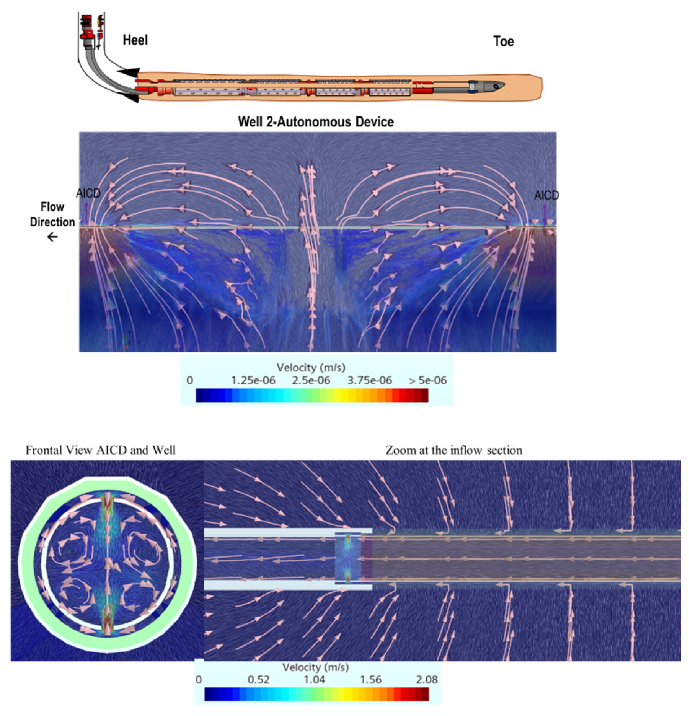
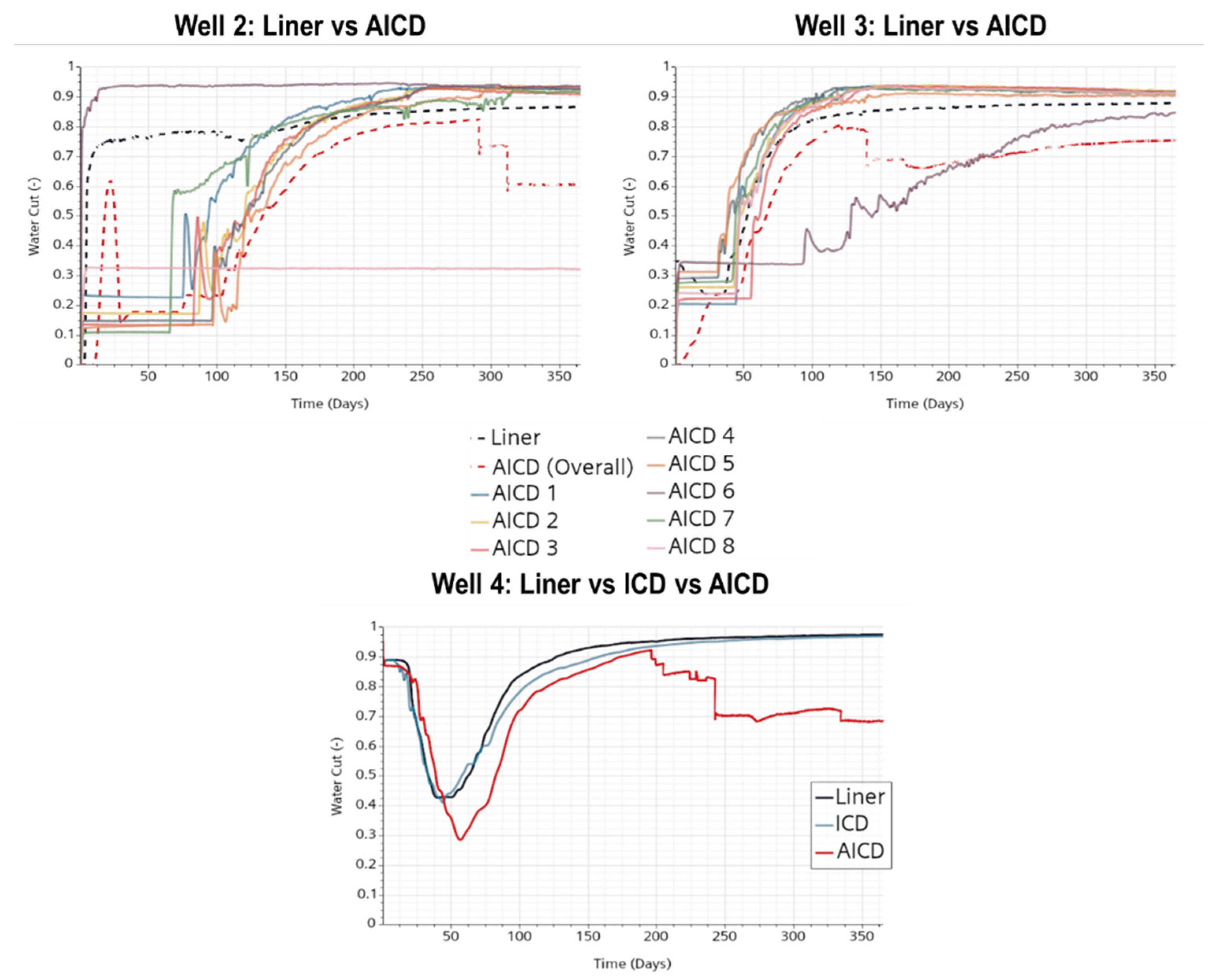
3.1.2. Well Internal Flow Hydrodynamic Behavior

One of the advantages of directly coupling the reservoir and the well with CFD modeling is the ability to describe the hydrodynamic behavior and integration between the reservoir, the annulus, and the well itself. This is particularly beneficial for capturing the dynamic changes in fluid properties within the well as the water-cut progressively increases, influencing the hydrodynamic profile along the well. Figure 11 illustrates an example of the velocity field and streamlined behavior in the Well 2 reservoir and the well after 500 days in a section completed with autonomous devices with pronounced channeling. Additionally, Figure 12 depicts the pressure profile for Well 4, utilizing ICD, to compare and illustrate the pressure gradients in the reservoir, completion, and the well.

Figure 11 presents the velocity profile and dominant streamlines and showcases the water movement profile in translucent blue. Initially, in the reservoir, velocities remain below $5\times {10}^{-6} \mathrm{m}/\mathrm{s}$, consistent with flow in porous media, with an increase observed near the inflow sections highlighted in yellow and red colors below the AICD labels. The streamlines indicate a preference for flow through already established water channels, capturing even the tortuosity caused by unstable displacement in some cases. This feature is particularly prominent in regions with the lowest pressure gradient, such as below the blank liner close to the aquifer. It underscores the consequences of interconnected water channels once they form during substantial, unstable displacements.

These pressure gradients are illustrated in Figure 12, including contour lines to highlight them, revealing that the lowest gradients occur below the blank liners. Although Figure 12 depicts Well 4, a similar trend is observed where unstable displacements cause severe water channeling far from the inflow zone. In this instance, the pressure drop between the well and the reservoir below the blank liners, at 3 ft below, was approximately 1 psi, emphasizing the severity of displacement instability in heavy oil wells even with relatively low force. Conversely, maximum pressure gradients are situated near the inflow zones, where the pressure drop between the reservoir and the well reaches up to 13 psi less than 3 ft below the inflow sand screen.

As the flow reaches the well, it enters through the sand screen. It changes direction perpendicularly to the annulus, flowing directly to the mechanical device compartment uniformly and homogeneously due to low velocities, averaging $1\times {10}^{-4} \mathrm{m}/\mathrm{s}$. Subsequently, it passes through the Water Mechanical Device, reaching the highest velocities caused by the reduction in flow area, reaching speeds up to 2 m/s in the studied cases. Finally, the flow exits the well perpendicularly, resulting in a significant perturbation to the flow. This collision of flows induces significant vortices in the well but quickly dissipates and uniformizes again. The velocity and pressure profiles in the well for the different studied cases are presented in Figure 13 at the breakthrough event (higher oil concentration) and after 500 days (higher water concentration), where flow perturbations are easily identifiable.

Well 1 exhibits a markedly distinct profile compared to the other wells regarding completion differences. Employing slotted liners, its velocity profile resembles typical pipeline flow. The velocity is at its lowest at the toe, gradually increasing through the heel. Noticeable jumps in velocity indicate the presence of blank liners, devoid of fluid inflow, characterized by a gentler slope. In comparison, sections with slotted liners feature a steeper slope due to inflow from the reservoir. Conversely, cases employing Downhole Water Mechanical Devices display discontinuities or jumps, signifying inflow through each valve or inflow device, particularly evident in Wells 2 and 3, which incorporate eight AICV sections. Nevertheless, overall profiles for these cases indicate a consistent behavior of increasing velocity from toe to heel due to fluid inflow. Finally, Well 4 exhibits a drop in flow velocity near the heel due to the inclusion of a long blank liner in its design of a bigger diameter (5 in vs. 4 in).

The pressure profile for the different wells, as depicted in Figure 13, reflects a typical pressure profile in pipelines. In contrast to velocity profiles, the slopes are smoother, with no discontinuities or sudden jumps. However, subtle slope changes indicate transitions between inflow and no-inflow (blank liner) zones. Additionally, the pressure drop along the well is discernible, with the highest pressure at the toe and the lowest at the heel, indicative of the expected pressure drop along the well. This pressure drop varies from 2 to 5 psi for the studied cases.

One of the key advantages of CFD simulations is their ability to visualize complex flow patterns and behaviors in scenarios where experimental methods are challenging or impractical. By generating detailed numerical simulations, CFD allows researchers to delve into intricate flow dynamics within confined spaces, porous media, or under extreme conditions. This capability is particularly advantageous when studying multiphase flows, turbulent regimes, or transient phenomena, where experimental data can be challenging to obtain or interpret. Moreover, CFD enables the exploration of a wide range of parameters and scenarios in a controlled computational environment, facilitating the optimization of designs and the development of new technologies. Figures S1 and S2 present the results for a horizontal well with an ICD, illustrating fluid movements in both the reservoir formation and the horizontal well completion.

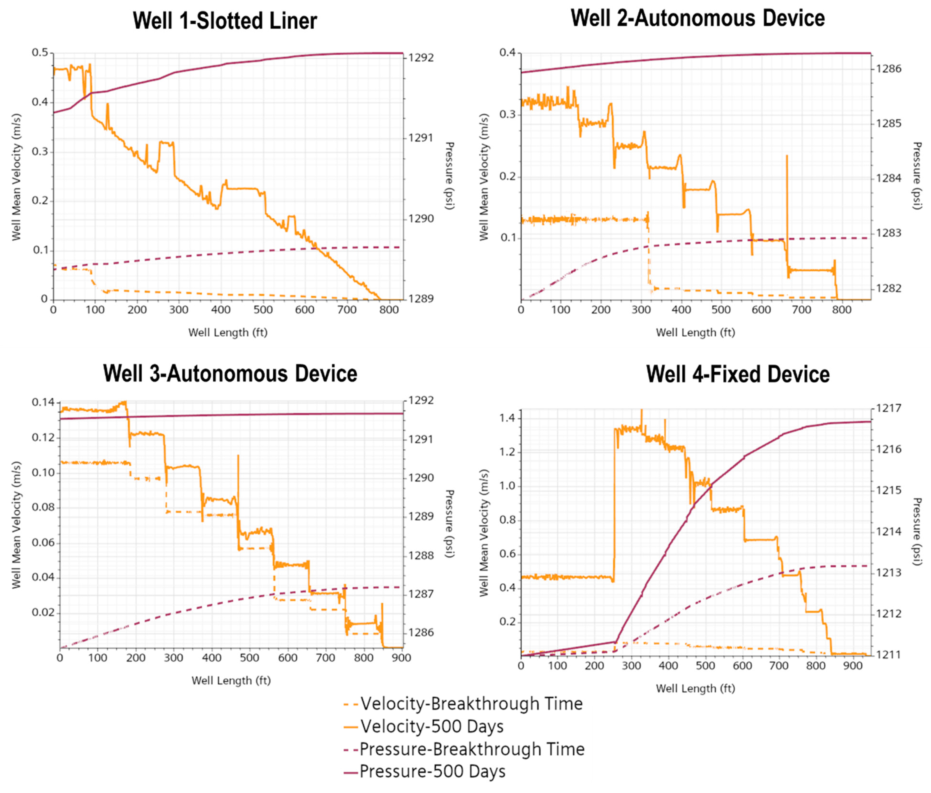
3.2. Production Profiles at Constant Drawdown

Numerical experiments were conducted at constant drawdown for three study cases to assess the advantages of various inflow technologies. Specifically, Wells 2 and 3 were compared using slotted liners versus autonomous control devices, while Well 4 underwent a comparison between slotted liners, AICD, and ICD. Figure 14 illustrates the production profiles for the different wells implementing these inflow technologies, while Figure 15 presents the cumulative production profiles.

Notably, the production profiles indicate significant improvements with AICD technologies. Across all three study cases, there was a noteworthy reduction in water production, ranging from 5.40 to 14.86 times less compared to the slotted liner technology. However, it is important to note that oil production was also affected following the choking of all valves, resulting in a reduction in oil production between 1.20 and 2.01 times compared to slotted liners.

On the contrary, Well 4, which compared three different completion technologies, revealed that ICD technology also reduced water production, albeit to a lesser extent than AICD. In this scenario, ICD resulted in 1.49 times less water production than slotted liners, whereas AICD proved more efficient, reducing water production by 12.26 times. Conversely, oil production favored slotted liners, followed by ICD, while AICD exhibited the lowest oil production due to valve choking. Specifically, ICD yielded 12.14% less oil than slotted liners, whereas AICD yielded 46.82% less oil.

The water-cut profiles over time for the different study cases are depicted in Figure 16. Results from Well 4 indicate that the water-cut profiles between ICD and slotted liners are similar and nearly overlapping. However, for AICD, the profiles exhibit a distinct behavior, presenting lower water-cuts over time, illustrating the benefits of choking water flow. The Water Oil Ratio (WOR) for slotted liners ranged between 12.39 and 18.16 for the studied cases. In contrast, it ranged between 2.17 and 2.75 for AICD and 10.76 for the ICD case, underscoring the significant reduction in water production with AICD.

Concerning the water production, Figure 16 illustrates the water-cut profiles per AICD for Wells 2 and 3. At the same time, Well 4 only presents the overall water-cut due to the higher number of devices (approximately 40). For Wells 2 and 3, water near the completion never migrated out of the inflow section. Upon water breakthrough in each inflow section, consequent channeling persisted, reaching values up to 90% in water-cut and remaining choked to reduce the inflow of fluids. This information could be helpful in the design of EOR strategies or the outflow of fluids from the well, aiming to migrate the water close to the inflow sections.

Regarding the carbon footprint, Figure 17 presents the $\mathrm{C}{\mathrm{O}}_2$ emission profiles for the different wells using different water inflow control technologies. Similar to the results previously presented in Section 3.1.1, carbon emissions are reduced when fixed or autonomous inflow technologies are implemented. For example, the fixed device study case reduced $\mathrm{C}{\mathrm{O}}_2$ emission $32.22\%$ compared to conventional slotted liners, while the autonomous devices reduced the carbon emissions between $67.80$ and $82.12\%$. Again, the reduction in the carbon footprint is attributed exclusively to a decrease in excessive water production and, in the AICD cases, to the choking of fluids, which avoids their exponential production.

Figure 18 illustrates the pressure and velocity profiles for the different study cases after 365 days. Notably, distinct variations between the completion technologies in these two variables are evident across all cases. For instance, AICD tends to exhibit a lower velocity profile than the other two completion technologies, which is attributed to the choking of the valves. Conversely, ICD and slotted liners technologies showcase higher velocity profiles in the well due to the larger inflow area they provide.

Regarding the pressure in the well, the profiles display consistent disparities related to the influence of the inflow technology, with the lowest pressure drop achieved with AICD due to the choking effect. However, ICD technology for Well 4 exhibited the most significant pressure gradient, 33% higher than its slotted liner counterpart, despite having the same drawdown.

4. Conclusions

• A validated 3-D CFD framework benchmarked slotted liners, passive inflow control devices (ICDs), and autonomous inflow control devices (AICDs) for heavy oil horizontal wells. The analysis focused on waterfront stability, production efficiency, and operations’ carbon intensity.
• Water-management performance. AICDs reduced cumulative water-cut by 81–93% compared to slotted liners, while ICDs achieved only a 33% reduction. Once AICD choking was initiated, valve closure remained stable, and no rebound in water production was detected.
• Production and well-count trade-off. The lower water-to-oil ratio delivered by AICDs can offset their modest loss in oil rate by allowing additional wells to be drilled without increasing total produced-water volumes (e.g., ≈18 extra wells to match the WOR of one slotted liner producer in the Well 2 case).
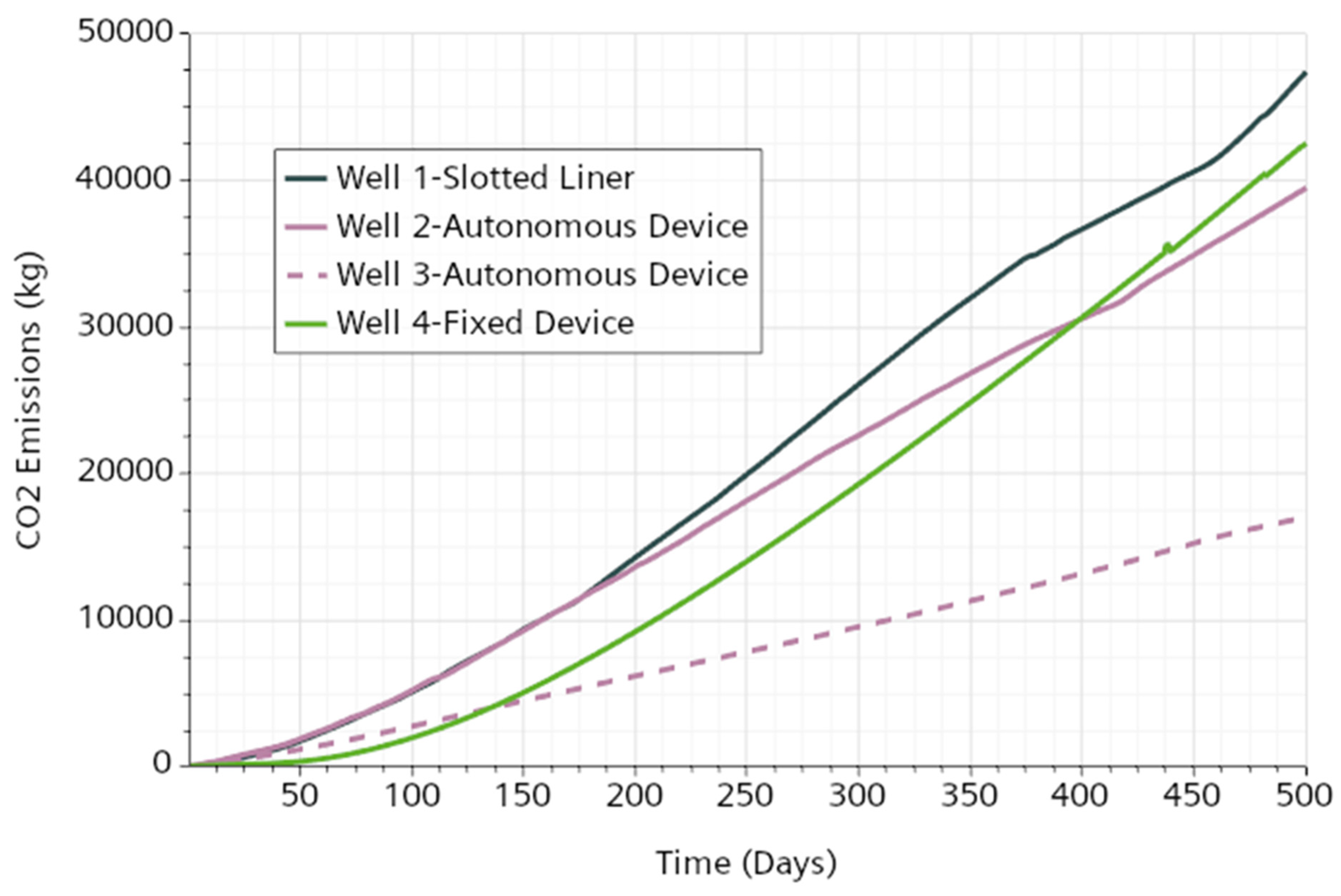
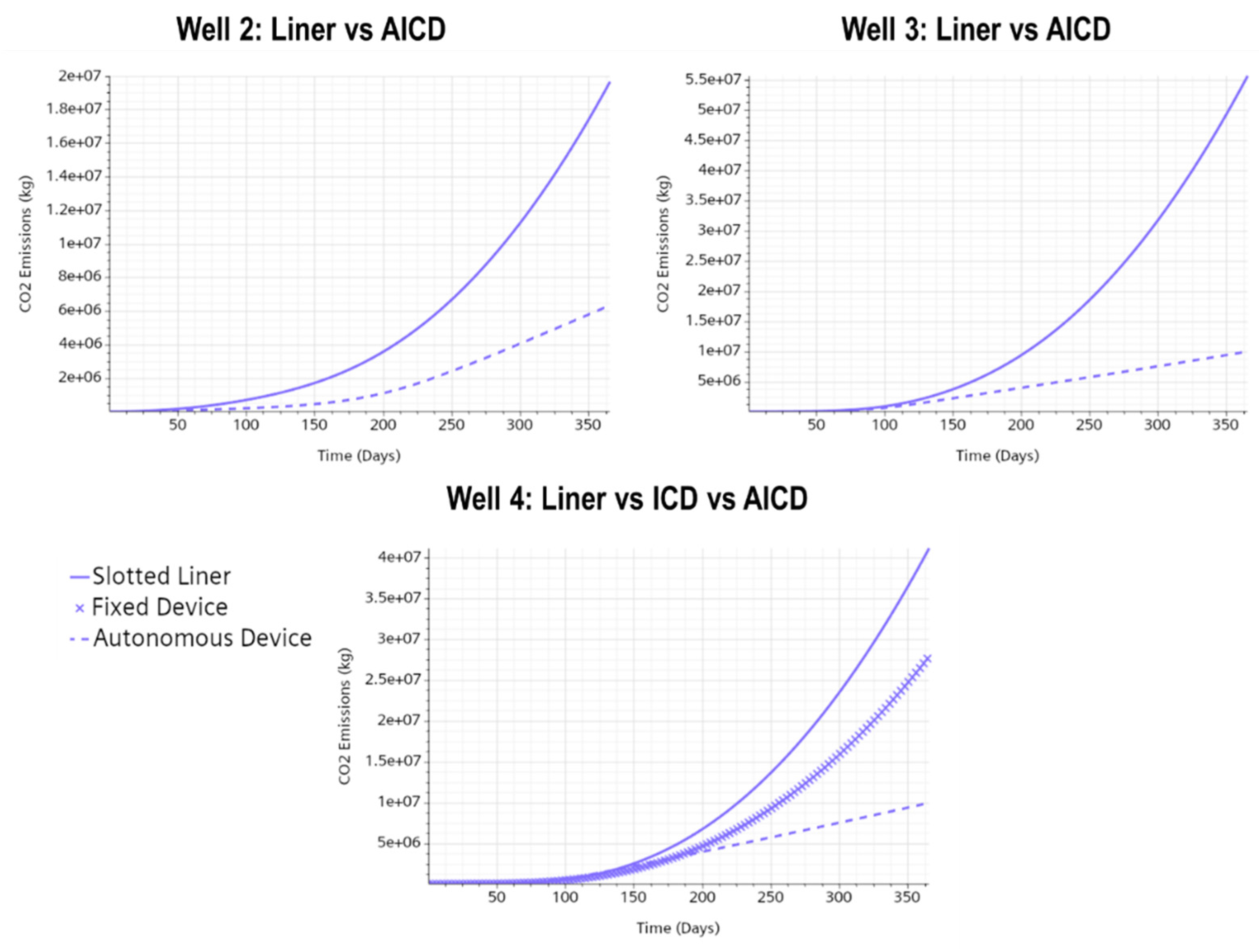
• Operational benefits and sustainability. AICDs decreased drawdown pressure by 18% and reduced life cycle CO₂ emissions per stock-tank barrel by up to 82%, highlighting their value in decarbonization strategies.
• Model validation and key design levers. Predicted oil and water rates matched production logs within ±14% and ±10%, respectively. Sensitivity studies confirm that nozzle diameter and the oil–water viscosity ratio are the primary design variables influencing AICD effectiveness.
• Field-deployment outlook. Pilot programs integrating distributed-temperature sensing with CFD-based optimization are recommended to fine-tune nozzle sizing and maximize long-term water control.

References

1. Daneshy, A.A. Selection and Execution Criteria for Water-Control Treatments. In Proceedings of the SPE International Symposium and Exhibition on Formation Damage Control, Lafayette, LA, USA, 15–17 February 2006. [Google Scholar] [CrossRef]
2. Farajzadeh, R.; Zaal, C.; Van den Hoek, P.; Bruining, J. Life-cycle assessment of water injection into hydrocarbon reservoirs using the exergy concept. J. Clean. Prod. 2019, 235, 812–821. [Google Scholar] [CrossRef]
3. Farajzadeh, R.; Kahrobaei, S.; Eftekhari, A.A.; Mjeni, R.A.; Boersma, D.; Bruining, J. Chemical enhanced oil recovery and the dilemma of more and cleaner energy. Sci. Rep. 2021, 11, 829. [Google Scholar] [CrossRef] [PubMed]
4. Al-Khelaiwi, F.T.; Davies, D.R. Inflow Control Devices: Application and Value Quantification of a Developing Technology. In Proceedings of the International Oil Conference and Exhibition in Mexico, Veracruz, Mexico, 27–30 June 2007. [Google Scholar] [CrossRef]
5. Fernandes, P.; Li, Z.; Zhu, D. Understanding the Roles of Inflow-Control Devices in Optimizing Horizontal-Well Performance. In Proceedings of the SPE Annual Technical Conference and Exhibition, New Orleans, LA, USA, 4–7 October 2009. [Google Scholar] [CrossRef]
6. Aadnoy, B.S.; Hareland, G. Analysis of Inflow Control Devices. In Proceedings of the SPE Offshore Europe Oil and Gas Conference and Exhibition, Aberdeen, UK, 8–11 September 2009. [Google Scholar] [CrossRef]
7. Brekke, K.; Lien, S.C. New, Simple Completion Methods for Horizontal Wells Improve Production Performance in High-Permeability Thin Oil Zones. SPE Drill. Complet. 1994, 9, 205–209. [Google Scholar] [CrossRef]
8. Coronado, M.P.; Garcia, L.; Russell, R.; Garcia, G.A.; Peterson, E.R. New Inflow Control Device Reduces Fluid Viscosity Sensitivity and Maintains Erosion Resistance. In Proceedings of the Offshore Technology Conference, Houston, TX, USA, 4–7 May 2009. [Google Scholar] [CrossRef]
9. Vela, I.; Viloria-Gomez, L.; Caicedo, R.; Porturas, F. Well Production Enhancement Results with Inflow Control Device (ICD) Completions in Horizontal Wells in Ecuador. In Proceedings of the SPE EUROPEC/EAGE Annual Conference and Exhibition, Vienna, Austria, 23–26 May 2011. [Google Scholar] [CrossRef]
10. Visosky, J.M.; Clem, N.J.; Coronado, M.P.; Peterson, E.R. Examining Erosion Potential of Various Inflow Control Devices to Determine Duration of Performance. In Proceedings of the SPE Annual Technical Conference and Exhibition, Anaheim, CA, USA, 11–14 November 2007. [Google Scholar] [CrossRef]
11. Youl, K.S.; Harkomoyo, H.; Suhana, W.; Regulacion, R.; Jorgensen, T. Passive Inflow Control Devices and Swellable Packers Control Water Production in Fractured Carbonate Reservoir: A Comparison with Slotted Liner Completions. In Proceedings of the SPE/IADC Drilling Conference and Exhibition, Amsterdam, The Netherlands, 1–3 March 2011. [Google Scholar] [CrossRef]
12. Cui, X.; Li, Y.; Li, H.; Luo, H.; Zhang, J.; Liu, Q. A Novel Automatic Inflow-Regulating Valve for Water Control in Horizontal Wells. ACS Omega 2020, 5, 28056–28072. [Google Scholar] [CrossRef] [PubMed]
13. Fripp, M.; Zhao, L.; Least, B. The Theory of a Fluidic Diode Autonomous Inflow Control Device. In Proceedings of the SPE Middle East Intelligent Energy Conference and Exhibition, Manama, Bahrain, 28–30 October 2013. [Google Scholar] [CrossRef]
14. Least, B.; Greci, S.; Burkey, R.; Ufford, A.; Wileman, A. Autonomous ICD Single Phase Testing. In Proceedings of the SPE Annual Technical Conference and Exhibition, San Antonio, TX, USA, 8–10 October 2012. [Google Scholar] [CrossRef]
15. Least, B.; Greci, S.; Wileman, A.; Ufford, A. Autonomous ICD Range 3B Single-Phase Testing. In Proceedings of the SPE Annual Technical Conference and Exhibition, New Orleans, LA, USA, 30 September–2 October 2013. [Google Scholar] [CrossRef]
16. Zeng, Q.; Wang, Z.; Wang, X.; Wei, J.; Zhang, Q.; Yang, G. A novel autonomous inflow control device design and its performance prediction. J. Pet. Sci. Eng. 2015, 126, 35–47. [Google Scholar] [CrossRef]
17. Zhao, L.; Least, B.; Greci, S.; Wileman, A. Fluidic Diode Autonomous ICD Range 2A Single-Phase Testing. In Proceedings of the SPE Oilfield Water Management Conference and Exhibition, Kuwait City, Kuwait, 21–22 April 2014. [Google Scholar] [CrossRef]
18. Crow, S.L.; Coronado, M.P.; Mody, R.K. Means for Passive Inflow Control Upon Gas Breakthrough. In Proceedings of the SPE Annual Technical Conference and Exhibition, San Antonio, TX, USA, 24–27 September 2006. [Google Scholar] [CrossRef]
19. Halvorsen, M.; Elseth, G.; Naevdal, O.M. Increased oil production at Troll is achieved through autonomous inflow control with RCP valves. In Proceedings of the SPE Annual Technical Conference and Exhibition, San Antonio, TX, USA, 8–10 October 2012. [Google Scholar] [CrossRef]
20. Halvorsen, M.; Madsen, M.; Vikøren Mo, M.; Isma Mohd, I.; Green, A. Enhanced Oil Recovery On Troll Field By Implementing Autonomous Inflow Control Device. In Proceedings of the SPE Bergen One Day Seminar, Bergen, Norway, 20 April 2016. [Google Scholar] [CrossRef]
21. Mathiesen, V.; Aakre, H.; Werswick, B.; Elseth, G. The Autonomous RCP Valve—New Technology for Inflow Control In Horizontal Wells. In Proceedings of the SPE Offshore Europe Oil and Gas Conference and Exhibition, Aberdeen, UK, 6–8 September 2011. [Google Scholar] [CrossRef]
22. Thornton, K.; Jorquera, R.; Soliman, M.Y. Optimization of Inflow Control Device Placement and Mechanical Conformance Decisions Using a New Coupled Well-Intervention Simulator. In Proceedings of the Abu Dhabi International Petroleum Conference and Exhibition, Abu Dhabi, United Arab Emirates, 11–14 November 2012. [Google Scholar] [CrossRef]
23. Timsina, R.; Furuvik, N.C.I.; Moldestad, B.M.E. Modeling and simulation of light oil production using inflow control devices. In Proceedings of the 58th Conference on Simulation and Modelling (SIMS 58), Reykjavik, Iceland, 25–27 September 2017. [Google Scholar] [CrossRef]
24. Archibong, C.; Erhiaganoma, E.; Ikehi, E. Optimization Study on Inflow Control Devices for Horizontal Wells in Thin Oil Column Reservoirs: A Case Study of a Well in Niger Delta. In Proceedings of the SPE Nigeria Annual International Conference and Exhibition, Lagos, Nigeria, 31 July–2 August 2017. [Google Scholar] [CrossRef]
25. Eltaher, E.K.; Muradov, K.; Davies, D.R.; Grebenkin, I.M. Autonomous Inflow Control Valves—Their Modelling and “Added Value”. In Proceedings of the SPE Annual Technical Conference and Exhibition, Amsterdam, The Netherlands, 27–29 October 2014. [Google Scholar] [CrossRef]
26. Amaratunga, M.; Perera, K.K.; Mathiesen, V.; Halvorsen, B.M. CFD simulation of a heavy oil reservoir with AICV completion. WIT Trans. Ecol. Environ. 2014, 190, 1227–1236. [Google Scholar] [CrossRef]
27. Haugen, T.E.; Elverhøy, A.B.; Mathiesen, V.; Halvorsen, B.M. Increasing oil recovery by utilization of AICV: A 3D multiphase simulation study of a heavy oil reservoir with an underlying water aquifer. WIT Trans. Ecol. Environ. 2014, 190, 1245–1254. [Google Scholar] [CrossRef]
28. Soltanian, M.R.; Amooie, M.A.; Gershenzon, N.; Dai, Z.; Ritzi, R.; Xiong, F.; Cole, D.; Moortgat, J. Dissolution Trapping of Carbon Dioxide in Heterogeneous Aquifers. Environ. Sci. Technol. 2017, 51, 7732–7741. [Google Scholar] [CrossRef]
29. Wijeratn, D.I.E.N.; Halvorsen, B.M. Computational Study of Heavy Oil Production with Inflow Control Devices. In Proceedings of the 56th Conference on Simulation and Modelling (SIMS 56), Linköping, Sweden, 7–9 October 2015; pp. 63–70. [Google Scholar] [CrossRef]
30. Pinilla, A.; Asuaje, M.; Pantoja, C.; Ramirez, L.; Gomez, J.; Ratkovich, N. CFD study of the water production in mature heavy oil fields with horizontal wells. PLoS ONE 2021, 16, e0258870. [Google Scholar] [CrossRef] [PubMed]
31. Byrne, M.; Jimenez, M.A.; Chavez, J.C. Predicting Well Inflow Using Computational Fluid Dynamics—Closer to the Truth? In Proceedings of the 8th European Formation Damage Conference, Scheveningen, The Netherlands, 27–29 May 2009. [Google Scholar] [CrossRef]
32. Byrne, M.; Jimenez, M.A.; Rojas, E.; Castillo, E. Computational Fluid Dynamics for Reservoir and Well Fluid Flow Performance Modelling. In Proceedings of the SPE European Formation Damage Conference, Noordwijk, The Netherlands, 7–10 June 2011. [Google Scholar] [CrossRef]
33. Byrne, M.; Jimenez, M.A.; Salimi, S. Modelling the Near Wellbore and Formation Damage—A Comprehensive Review of Current and Future Options. In Proceedings of the SPE European Formation Damage Conference, Noordwijk, The Netherlands, 7–10 June 2011. [Google Scholar] [CrossRef]
34. Byrne, M.T.; Jimenez, M.A.; Rojas, E.A.; Chavez, J.C. Modelling Well Inflow Potential in Three Dimensions Using Computational Fluid Dynamics. In Proceedings of the SPE International Symposium and Exhibition on Formation Damage Control, Lafayette, LA, USA, 10–12 February 2010. [Google Scholar] [CrossRef]
35. Yang, M.; Li, H.; Xie, J.; Wang, Y.; Jiang, R.; Zhu, S.; Li, Y. The theory of the automatic phase selection controller and its performance analysis. J. Pet. Sci. Eng. 2016, 144, 28–38. [Google Scholar] [CrossRef]
36. Zhang, N.; Li, H.; Liu, Y.; Shan, J.; Tan, Y.; Li, Y. A new autonomous inflow control device designed for a loose sand oil reservoir with bottom water. J. Pet. Sci. Eng. 2019, 178, 344–355. [Google Scholar] [CrossRef]
37. Garcia, L.; Coronado, M.P.; Russell, R.D.; Garcia, G.A.; Peterson, E.R. The First Passive Inflow Control Device That Maximizes Productivity During Every Phase of a Well’s Life. In Proceedings of the International Petroleum Technology Conference, Doha, Qatar, 7–9 December 2009. [Google Scholar] [CrossRef]
38. Zhao, L.; Zeng, Q.; Wang, Z. Design and Performance of a Novel Autonomous Inflow Control Device. Energy Fuels 2018, 32, 125–131. [Google Scholar] [CrossRef]
39. Corona, G.; Yin, W.; Felten, F. Enhanced Nozzle Inflow Control Device Development for Wall Shear Stress Minimization in High-Production Application. In Proceedings of the Offshore Technology Conference, Houston, TX, USA, 2–5 May 2016. [Google Scholar] [CrossRef]
40. Dong, L.-L.; Zhang, Y.-L. Analysis and experimental study on resistance-increasing behavior of composite high efficiency autonomous inflow control device. Pet. Sci. 2023, 21, 1290–1304. [Google Scholar] [CrossRef]
41. Cerquera, L.A.R.; Pinilla, J.A.; Ratkovich, N.R.; Asuaje, M. Study of the Dynamic Behavior of an Autonomous Inflow-Control Device Using a Digital Twin. Processes 2022, 10, 2691. [Google Scholar] [CrossRef]
42. Pinilla, A.; Stanko, M.; Asuaje, M.; Ratkovich, N. In-Depth Understanding of ICD Completion Technology Working Principle. Processes 2022, 10, 1493. [Google Scholar] [CrossRef]
43. Da Silva, D.V.A.; Jansen, J.D. A Review of Coupled Dynamic Well-Reservoir Simulation. IFAC-PapersOnLine 2015, 48, 236–241. [Google Scholar] [CrossRef]
Figure 1. Reservoir heterogeneity: (a) Well 1—slotted liner, (b) Well 2—AICD, (c) Well 3—AICD, and (d) Well 4—ICD (0.5 ft logging resolution).
Processes 13 01576 g001
Figure 2. Description of the well’s completion, initial, and boundary conditions.
Processes 13 01576 g002
Figure 3. General overview of the mesh implemented in the CFD model.
Processes 13 01576 g003
Figure 4. The water flows from the reservoir and displaces the front of the wells during the breakthrough event.
Processes 13 01576 g004
Figure 5. Aquifer disturbance and displacement front in the different wells after 500 days.
Processes 13 01576 g005
Figure 6. Examples of substantial unstable displacement. Blue iso-surfaces denote water saturation > 0.9.
Processes 13 01576 g006
Figure 7. Water-cut profiles measured 1 ft below the well: Blue label indicates initial water breakthrough and purple label after 500 production days.
Processes 13 01576 g007
Figure 8. Production profiles for the different wells compared to normalized field data.
Processes 13 01576 g008
Figure 9. Normalized accumulated production for the different case studies.
Processes 13 01576 g009
Figure 10. Cumulative C O 2 emissions for the different study cases.
Processes 13 01576 g010
Figure 11. Example of the hydrodynamic profile for Well 2 after 500 days.
Processes 13 01576 g011
Figure 12. Example of the pressure profile for Well 4 after 500 days.
Processes 13 01576 g012
Figure 13. Wellbore flow at breakthrough (upper half) and +500 days (lower half).
Processes 13 01576 g013
Figure 14. Production profiles for the different study cases comparing inflow technologies.
Processes 13 01576 g014
Figure 15. Accumulative production profiles for the different study cases comparing inflow technologies.
Processes 13 01576 g015
Figure 16. Water-cut profiles for the different completion technologies and some individual AICDs.
Processes 13 01576 g016
Figure 17. Cumulative carbon footprint for the different studied cases.
Processes 13 01576 g017
Figure 18. Mean average velocity and pressure profiles in the well for the different study cases after 365 days.
Processes 13 01576 g018