Optimization of Process Parameters for Wire Electrical Discharge Machining of 9Cr18Mov Based on Grey Relational Analysis

Abstract

9Cr18MoV stainless steel is widely employed in cutting-tool applications owing to its exceptional hardness and corrosion resistance. In this study, we systematically optimized the wire electrical discharge machining (WEDM) process parameters for 9Cr18MoV stainless steel through an L₁₆ (4⁴) orthogonal experimental design. The key parameters investigated include pulse width (T_on), pulse interval (T_off), peak current (IP), and wire feed speed (WS), with cutting efficiency (CE) and surface roughness (R_a) serving as the primary optimization objectives. A signal-to-noise ratio (SNR) analysis was applied to assess the effects of the individual parameters and derive single-objective optimal configurations. Subsequently, grey relational analysis (GRA) integrated with analytic hierarchy process (AHP)-based weighting was employed to establish a multi-objective optimal parameter set, which was experimentally validated. The results reveal that the optimal multi-objective performance was attained at T_on = 28 μs, T_off = 3 μs, IP = 9 A, and WS = level 3. SEM characterization confirmed that this parameter combination yields a more uniform surface morphology, with diminished oxidation and molten debris deposition, thereby significantly enhancing surface integrity. The adoption of this optimized parameter set not only ensures superior machining efficiency but also results in improved surface quality.

1. Introduction

Wire electrical discharge machining (WEDM) is widely used in the processing of molds, precision parts, and special materials due to its advantages, namely, high dimensional accuracy, fast machining speed, and high material utilization [1]. Its working principle involves the use of electrical sparks generated between the electrode wire and the workpiece at a microscopic distance to erode the material being processed. Throughout the machining process, direct physical contact and frictional interaction between the tool electrode and workpiece material are completely eliminated. As a result, WEDM is not constrained by the mechanical properties of the material being processed, enabling the machining of materials of any hardness, strength, or brittleness. Among these materials is 9Cr18MoV steel, a metal that is known for its excellent corrosion resistance and exhibits high viscosity and a rapid temperature rise during machining [2]. It is a high-carbon chromium stainless steel belonging to the martensitic stainless steel series. 9Cr18MoV is widely used in the manufacture of various cutting tools, blades, surgical instruments, and dental tools in the medical field [3]. It is also applied in the aerospace and military industries for highly wear-resistant components. Additionally, 9Cr18MoV is recognized as a premium stainless steel on the tool market.

In the field of utilizing WEDM for processing hard and high-strength metallic materials, researchers have conducted extensive studies. Sun et al. [4] reviewed the progress in the WEDM of difficult-to-machine materials, particularly hard metals and composites. Their research emphasized the influence of parameters such as pulse width, wire tension, and the dielectric fluid used on machining efficiency and overall process quality. Li et al. [5] explored the application of WEDM for machining the superalloy IN 718, demonstrating the use of hybrid cooling techniques to improve surface integrity and reduce electrode wear. Arikatla et al. [6] investigated the application of WEDM in titanium alloy machining, identifying optimal process parameters to minimize electrode wear (EWR) and enhance cutting efficiency (CE). Li et al. [7] focused on the evolution of surface integrity and machining efficiency during the WEDM of the nickel-based alloy IN 718. Their results showed that WEDM technology can achieve high material removal rates (MRRs); the six-sigma distribution of surface roughness (R_a) in rough-cutting mode differs from that in trim-cutting mode; and the high toughness of IN 718 is the primary reason for the absence of microcracks in trim-cutting mode. Antar et al. [8] studied experimental data on workpiece productivity and integrity during the WEDM of the nickel-based superalloy Udimet 720 and the titanium alloy Ti-6Al-2Sn-4Zr-6Mo. Compared to uncoated brass wire machined using the same operating parameters, productivity increased by up to 70%, and after two trim cuts, the R_a reached 0.6 μm, with residual stresses close to neutral and the recast layer nearly eliminated.

Regarding the optimization of WEDM parameters for metals and composites, Asgar et al. [9] outlined current research trends in WEDM. Numerous process parameters (e.g., pulse width, pulse interval, etc.) can be adjusted to improve various performance metrics (e.g., MRR and R_a). Their study demonstrated that different optimization techniques (e.g., the Taguchi method, grey relational analysis (GRA), and analysis of variance (ANOVA) are applicable to a variety of materials, including alloys, superalloys, and metal matrix composites. Natarajan et al. [10] investigated parameter optimization for the WEDM of stainless steel, considering pulse interval, pulse width, voltage, and average current as electrical parameters. They employed orthogonal experiments, ANOVA, and GRA to optimize the experimental results and analyze the optimal combination of process parameters for achieving the best MRR and surface roughness. Mahapatra et al. [11] used Taguchi parameter design to identify critical machining parameters affecting the performance metrics of D2 tool steel, including discharge current, pulse width, pulse frequency, wire speed, and wire tension. Through nonlinear regression analysis, they established relationships between machining parameters and responses such as MRR, surface finish, and kerf width, thereby developing effective mathematical models. The optimization process was ultimately completed through the use of a genetic algorithm, which enabled the simultaneous optimization of multiple performance metrics and the identification of the optimal machining parameter configuration.

Previous research findings have substantiated the effectiveness of WEDM technology in processing diverse composite materials and hard alloys [12]. Moreover, the implementation of advanced optimization methodologies has been shown to significantly improve the machining performance of WEDM for these challenging materials. This study focuses on the application of WEDM technology for machining 9Cr18MoV stainless steel, with the primary objective being to optimize process parameters to simultaneously enhance cutting efficiency (CE) and reduce surface roughness (R_a). In the experimental framework, we incorporated an orthogonal design methodology for systematic planning. The signal-to-noise ratio (SNR) analytical approach was employed to quantitatively assess the effects of four critical parameters—pulse width, pulse interval, peak current, and wire feed speed—on the machining performance regarding 9Cr18MoV. Additionally, grey relational analysis (GRA) was employed to develop a robust multi-criteria evaluation system, facilitating the determination of optimal process parameters through multi-objective optimization.

2. Experiments and Methods

The metal material selected for this study is 9Cr18MoV. The elemental composition and performance parameters of 9Cr18MoV stainless steel are presented in

Table 1. Elemental composition of 9Cr18MoV stainless steel.

Elements	C	Si	Mn	P	S	Cr	Ni	Mo	V	Fe
Weight%	0.85~0.95	≤0.8	≤0.8	≤0.035	≤0.03	17~19	≤0.6	1~1.3	0.07~0.12	Others

and

Table 2. Mechanical properties of 9Cr18MoV.

Parameter	Value
Melting Point (°C)	1360–1400 °C
Elastic Modulus (GPa)	200 Gpa
Coefficient of Thermal Expansion	10.5–115
Thermal Conductivity W/(m·K)	16–24
Density (g/cm3)	7.75–7.8
Tensile Strength (MPa)	1000
Yield Strength (MPa)	760
Hardness (Annealed State) (HB)	≤269
Hardness (Quenched State) (HRC)	≥58

. After being quenched, its hardness typically exceeds 58 HRC, which increases the difficulty of mechanical machining. Furthermore, this material exhibits excellent corrosion resistance, moderate magnetic properties, and high toughness [13].

The experimental 9Cr18MoV specimens prepared had initial dimensions of 60 × 60 × 16 mm (length × width × height). After being obtained through commercial purchases, the material was forged. After the WEDM process, the machined samples exhibited final dimensions of 25 × 16 × 3 mm (length × width × height), as illustrated in Figure 1a. A total of 16 groups were processed in this experiment, and each group was subjected to the experiment 3 times, so a total of 48 samples were made. SEM and an EDS scanning electron microscope were used to observe and analyze the surfaces of the processed samples. We used a Sigma500 field (Carl Zeiss AG, Oberkochen, Germany) emission scanning electron microscope equipped with an energy spectrum scanner, which provides exceptional resolution capabilities for observing material microstructures within the 0.1 to 100 nm range. The instrument’s depth of field surpasses that of transmission electron microscopes by a factor of 10 and that of optical microscopes by several hundredfold. The SEM analysis results, including surface morphology and chemical composition, are presented in Figure 1b,c, respectively. R_a measurements were conducted by using a TR200 profilometer (Guangzhou Junda Instrument Co., Ltd., Guangzhou, China) to quantitatively evaluate the surface properties of the WEDM-processed 9Cr18MoV specimens.

For the experimental machining, an HF320MZQ-G20 medium-speed wire-cut EDM machine, developed by Hangzhou Huafang CNC Machine Tool Co., Ltd., Hangzhou, China, was utilized. The maximum cutting efficiency of the machine tool is ≥180 mm²/min, and the maximum roughness can reach R_a ≤ 1.0 um after multiple cuttings. The overall setups of the machine and the machining site are shown in Figure 2. The tool electrode wire used was a molybdenum wire with a diameter of 0.18 mm. The working fluid was a commercially available water-based solution, supplied in spray mode during the machining process.

The working principle of processing a material using WEDM is illustrated in Figure 3. The macroscopic discharge process occurring during machining is shown in Figure 3a, and the microscopic machining process mainly includes the following stages [14].

Ionization preparation stage (Figure 3b): When a voltage is applied between the electrodes, an electric field is formed. Under the influence of this electric field, the working fluid becomes polarized. As the strength of the electric field increases, positively charged ions move rapidly toward the wire electrode, while negatively charged electrons accelerate toward the workpiece electrode, colliding with molecules in the working fluid and causing ionization [14].

Discharge channel formation stage (Figure 3c): As the strength of the electric field continues to increase, it eventually reaches a specific threshold, and thus the working fluid medium is instantaneously broken down, forming a discharge channel. Within this channel, electrical energy is rapidly converted into thermal energy, which is released along the channel onto the surfaces of the electrodes, causing the temperature to rise sharply to tens of thousands of degrees Celsius in an extremely short time.

Material ejection stage (Figure 3d): The intense heat causes the material in the machining zone of the workpiece to erode. Simultaneously, the interface between the discharge channel and the neutral gas separates, forming bubbles [14].

Deionization stage (Figure 3e): After the discharge ends, positive and negative particles in the channel quickly neutralize, leading to deionization. The bubbles continue to expand due to the inertia of the working fluid, while the molten workpiece material evaporates rapidly under low pressure and detaches from the surface of the workpiece. However, a small portion of the eroded material may re-splash and adhere to the surfaces of both the tool electrode and the workpiece. This concludes the entire discharge erosion process [15].

In wire electrical discharge machining (WEDM) technology, numerous process parameters influence the machining speed and surface quality of 9Cr18MoV material. Based on the insights from previous studies [16], this research primarily focuses on the following four process parameters, which have a significant impact on machining performance: pulse width (T_on), pulse interval (T_off), peak current (IP), and wire feed speed (WS) (adjusted in levels, with speeds ranging from 1.17 to 11.17 m/s). The CE and R_a were selected as the key performance indicators for the experiments. Their calculation formulas are provided in Equations (1) and (2), respectively [17].

$$\mathrm{CE}={\displaystyle \frac{\mathrm{LH}}{\mathrm{t}}}$$

(1)

Equation (1): Expression for CE.

$${\mathrm{R}}_{\mathrm{a}}={\displaystyle \frac{{\mathrm{R}}_{\mathrm{a}1}{,\mathrm{R}}_{\mathrm{a}2}\dots {\mathrm{R}}_{\mathrm{an}}}{\mathrm{n}}}$$

(2)

Equation (2): Expression for R_a.

In Equation (1), L represents the length of the perimeter of the workpiece being cut (unit: mm), H denotes the thickness of the workpiece (unit: mm), and t is the time taken to cut the perimeter of the workpiece (unit: min). In Equation (2), R_an represents the R_a measured during the n-th measurement (unit: μm), and n is the number of measurements (n ≥ 3).

Different combinations of process parameters at various levels can have varying impacts on experimental results. Therefore, based on statistical analysis and considering the different combinations of levels for each factor, an L₁₆ (4⁴) orthogonal experimental design was adopted. The orthogonal experimental factors and levels are shown in

Table 3. Orthogonal experimental parameters and levels.

Process Parameters	Unit	Symbol	Level
			1	2	3	4
Pulse Width	μs	Ton	12	20	28	36
Pulse gap	μs	Toff	3	5	7	9
Peak current	A	IP	5	7	9	11
Wire speed	Gear	WS	0	1	2	3

. This design allows for the analysis of the influence of each factor on the machining indicators using the minimum number of experiments. In the WEDM of 9Cr18MoV, the optimal machining indicators are the lowest R_a and the highest CE. However, in practice, it is often challenging to simultaneously achieve optimal levels for both R_a and CE [18]. Thus, the grey relational analysis (GRA) method is employed to optimize the process parameter combinations for multi-objective optimization, yielding the optimal parameter combination scheme [19].

3. Experimental Results and Analysis

3.1. Surface Topography and Roughness

Figure 4 presents the SEM results regarding the morphology of the machined surface under two different working conditions. There are some similarities between the SEM results for 9Cr18MoV stainless steel and those for pure metals such as tungsten titanium, including microcracks, microspheres, and microvias. During WEDM, a significant amount of heat is instantaneously generated, reaching extremely high temperatures (6000–10,000 °C), causing localized melting and vaporization of metal. The volcanic lava-like crenelation morphology on the sample surface is formed by the rapid cooling of the surface of the material under the influence of discharge energy, resulting in a recast layer [20].

Comparative analysis of the SEM images reveals distinct differences in surface morphology between Figure 4a,b. The combination of machining process parameters in Figure 4a is T_on = 36 μs, T_off = 3 μs, IP = 11 A, and WS = 4; the combination of machining process parameters in Figure 4b is T_on = 36 μs, T_off = 7 μs, IP = 7 A, and WS = 6. The surface in Figure 4a exhibits significantly greater complexity, characterized by a higher density of microspheres, micropores, and adhered debris particles. This morphological variation is primarily due to enhanced discharge energy associated with increased peak current levels, which generates a substantial amount of thermal energy during the machining process. These elevated thermal conditions promote the extensive melting and vaporization of the stainless steel material [21]. These thermal effects ultimately compromise the material’s surface integrity, manifesting as increased R_a values.

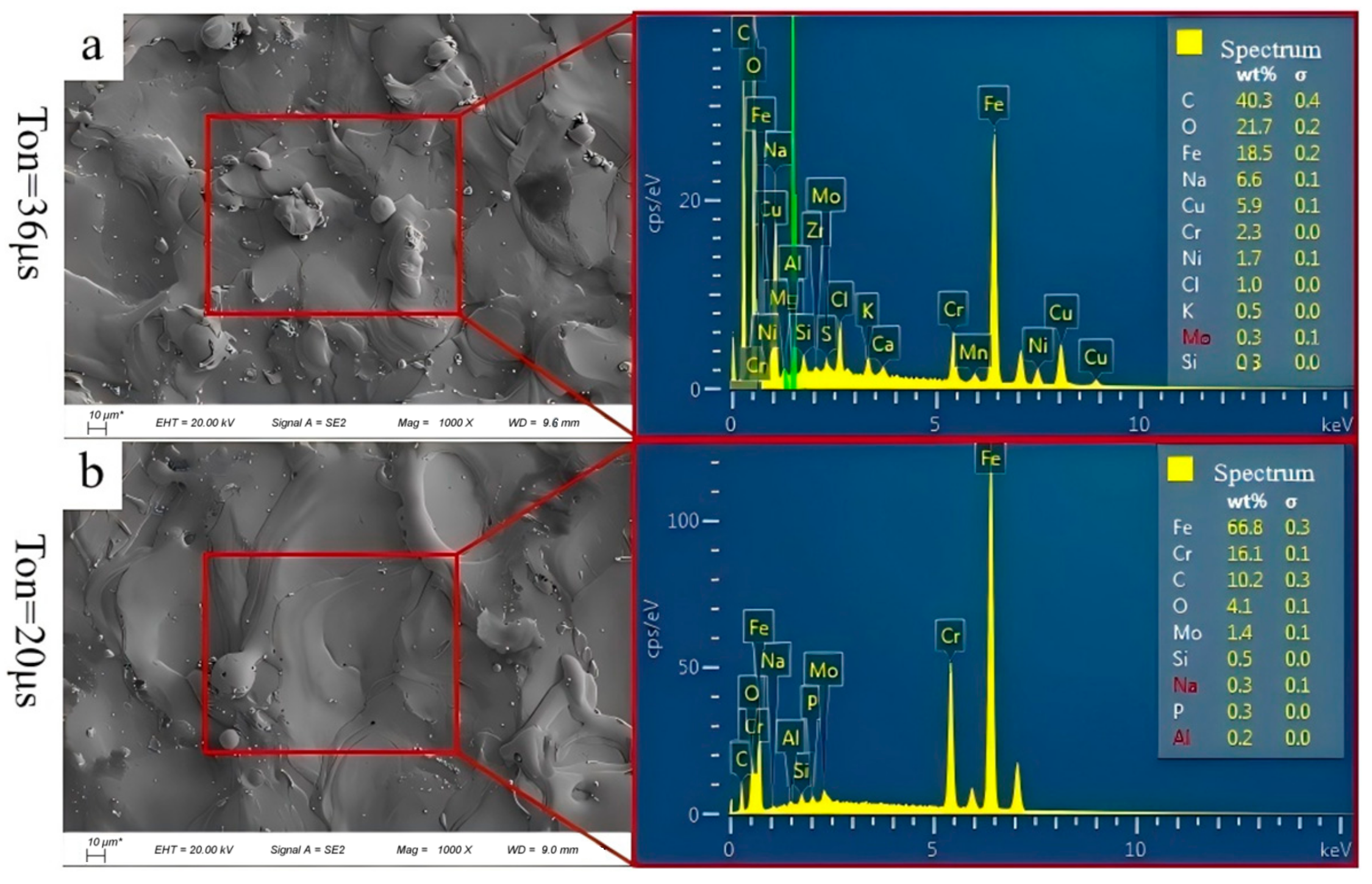
Figure 5 presents a comparison of SEM images of the machined surfaces under pulse widths of 36 μs and 20 μs, respectively. Through comparative analysis, it is evident that the surface morphology in (b) (T_on = 20 μs) is significantly smoother than that in (a) (T_on = 36 μs). Defects such as microspheres, micropores, and protrusions are notably reduced in the right image [22]. This phenomenon can be attributed to changes in discharge energy: as T_on increases, the discharge energy also increases, leading to a significant rise in the heat released during the machining process. Under these conditions, the 9Cr18MoV material undergoes more pronounced melting and vaporization, resulting in a greater accumulation of substrate material upon cooling and ultimately forming a rougher surface morphology [23]. Additionally, based on the EDS image on the left, the content of metallic elements such as Fe and Cr decreases under high-pulse conditions, as these elements are more prone to oxidation or evaporation at high temperatures. In contrast, the Mo content remains relatively stable, while the O content increases. This change can be attributed to the thickening of the surface oxide layer and the increase in oxide content as the pulse width increases, leading to a relative reduction in metallic element content. These results indicate that pulse width has a significant impact on surface quality, with lower pulse widths contributing to a smoother surface morphology.

3.2. Surface Recast Layer

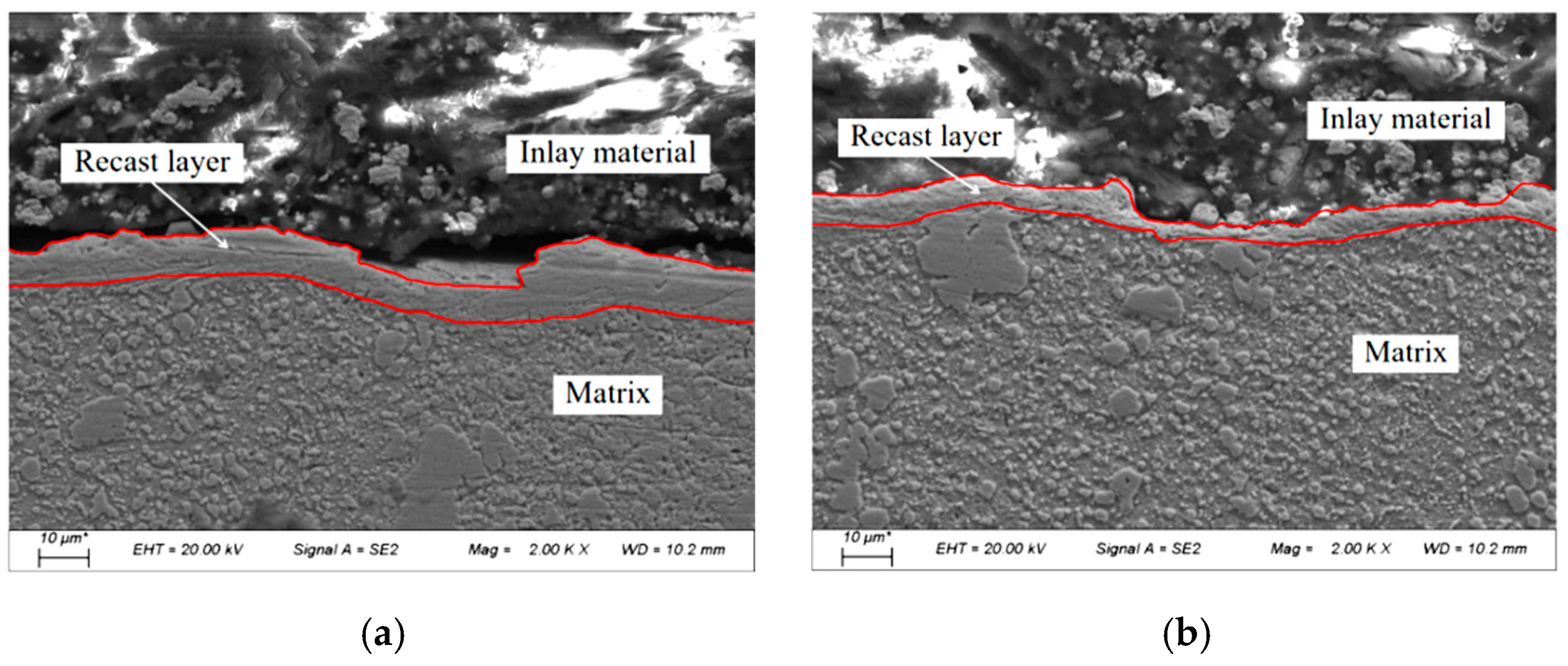
After WEDM, the recast layer on a material’s surface exhibits unique and complex morphological characteristics. The recast layer generally covers the machined surface but shows variations in thickness in certain areas. The surface is not entirely smooth but displays a certain degree of undulation, resembling a “hilly terrain” at a microscopic scale.

In this experiment, a total of eight groups of sample recasting layers were measured, and two typical recasting layers were selected, as shown in Figure 6, for analysis. In the images, it can be observed that the recast layer in Figure 6a is thicker than that in Figure 6b, with more pronounced microscopic protrusions and depressions. These protrusions and depressions have sharp edges and irregular shapes, further exacerbating surface unevenness and resulting in a higher R_a value for the layer in Figure 6a. The thicker recast layer in Figure 6a is likely due to this layer’s higher IP compared to that in Figure 6b, injecting more energy into the workpiece surface during discharge pulses. This leads to deeper discharge craters [24]. The deepening of discharge craters increases the volume of metal debris within the discharge gap, reducing the breakdown strength of the working fluid. After the discharge ends, the melted and vaporized material cools and solidifies, causing more debris to accumulate on the surface and increasing the thickness of the recast layer. Additionally, the heat generated during discharge cannot be fully expelled with the debris, leading to heat accumulation and repeated discharges at the same locations, further deteriorating the machining environment. However, if the IP is too low, the discharge energy becomes insufficient, reducing the amount of melting and vaporization on the material’s surface and resulting in a thinner recast layer. This may lead to issues such as low machining efficiency [25]. Therefore, in practical WEDM applications, it is essential to carefully control electrical parameters to achieve ideal process metrics and machining outcomes.

3.3. Signal-to-Noise Ratio Analysis

To minimize the interference of random factors in repeated experiments and extract as much valid information as possible from the experimental results, the SNR analysis method was introduced. By calculating the SNR values corresponding to each set of experimental results, data analysis can be performed to account for controllable factors while reducing the influence of random disturbances, thereby improving the accuracy of the computational analysis. In the SNR method, system responses are categorized into three types: nominal is the best, the larger the better, and the smaller the better. For CE, a larger value is desirable, so the larger-the-better characteristic is applied, and the SNR can be calculated using Equation (3). For R_a, a smaller value is preferred, so the smaller-the-better characteristic is used, and the SNR can be calculated using Equation (4). A higher SNR value indicates better experimental results.

$$\mathrm{S}/\mathrm{N}=-10\ast \lg ({\displaystyle \frac{1}{\mathrm{n}}}{\displaystyle {\sum }_{\mathrm{i}=1}^{\mathrm{n}}\frac{1}{{{\mathrm{y}}_{\mathrm{i}}}^2}})$$

(3)

Equation (3): The larger the better.

$$\mathrm{S}/\mathrm{N}=-10\ast \lg ({\displaystyle \frac{1}{\mathrm{n}}}{\displaystyle {\sum }_{\mathrm{i}=1}^{\mathrm{n}}{{\mathrm{y}}_{\mathrm{i}}}^2})$$

(4)

Equation (4): The smaller the better.

In the formulae, S/N represents the signal-to-noise ratio (SNR) of the process target, n is the total number of experimental samples (in this study, n = 16), and y_i is the sample data for the i-th level factor. In the Taguchi analysis response table, the difference between the maximum and minimum average response values for a factor is referred to as Delta. A larger Delta value for a given factor indicates that it has a greater influence on the evaluation metric, and thus the factor ranks higher in importance [26].

By substituting the experimental results regarding CE and R_a into the respective formulas, the corresponding SNR values were calculated, as shown in

Table 4. Optimization metrics’ signal-to-noise ratio values.

No.	Signal-to-Noise Ratio
	CE	Ra
1	30.263	−2.049
2	27.572	−2.997
3	27.389	−6.600
4	28.743	−4.464
5	34.054	−6.596
6	31.017	−6.307
7	31.822	−7.024
8	20.170	−0.906
9	35.485	−4.915
10	34.117	−8.379
11	21.649	−4.286
12	29.562	−5.235
13	31.750	−12.089
14	31.205	−4.297
15	32.546	−8.711
16	20.284	−5.818

. Since each factor has four levels and there are 16 experimental groups in total, each level corresponds to four sets of SNR values.

The mean SNR values for CE were calculated for each level of each factor based on the corresponding four experimental groups, and the results are plotted in Figure 7. In Figure 7, the following trends can be observed: As T_on increases, CE initially rises and then decreases. As T_off increases, CE shows a declining trend. As IP increases, CE initially rises and then stabilizes. As WS increases, CE first decreases and then increases. Additionally, the plots indicate that the IP has the largest range of mean SNR values, suggesting that IP has the most significant influence on CE. This is because the peak current determines the energy intensity of a single pulse. A higher peak current implies greater energy release, which can melt the material more rapidly, thereby improving CE.

The optimal parameter combination for maximizing CE was determined by selecting the levels corresponding to the highest mean SNR values for each factor. The optimal parameter combination is as follows: T_on: 28 μs, T_off: 3 μs, IP: 11 A, and WS: Level 3.

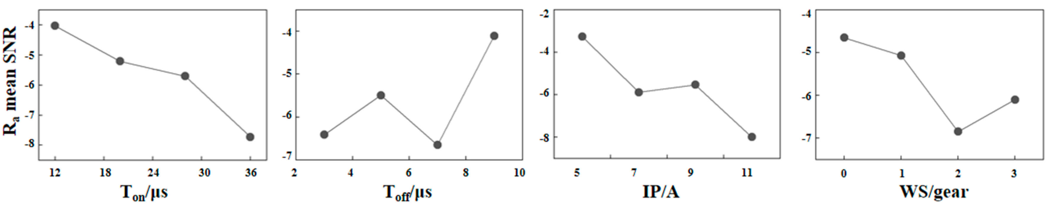
The mean SNR values for R_a were calculated for each level of each factor based on the corresponding four experimental groups, and the results are plotted in Figure 8. In Figure 8, the following trends can be observed: As T_on increases, R_a shows a declining trend. As T_off increases, R_a initially rises, then decreases, and finally rises again. As IP increases, R_a first decreases and then increases. As WS increases, R_a gradually decreases. Furthermore, the plots indicate that the IP has the largest range of mean SNR values, suggesting that IP has the most significant influence on R_a. This is because a higher peak current generates larger discharge craters, leading to an increase in R_a. Therefore, the greater the peak current, the more pronounced the surface roughness. The optimal parameter combination for minimizing R_a was determined by selecting the levels corresponding to the highest mean SNR values for each factor. The optimal parameter combination is as follows: T_on: 12 μs, T_off: 9 μs, IP: 5 A, and WS: Level 0.

3.4. Grey Correlation Method for Multi-Objective Optimization Analysis

For different evaluation dimensions, the influence of factors varies. That is, the optimal factor combination for surface roughness may not necessarily be the best for cutting speed [27]. In practical WEDM of 9Cr18MoV, it is essential to consider both CE and R_a comprehensively. Therefore, multi-objective optimization analysis is necessary. In this study, we employed the GRA method, a multi-factor statistical analysis approach in which sample data are used to describe the strength, magnitude, and order of relationships between factors through grey relational degrees. The calculation process for grey relational degrees is as follows [28]: The comparison sequence consists of a set of data under the two optimization indicators in Table 4, where x_e(k) represents the SNR values for CE and R_a, respectively. Here, e = 1, 2: When e = 1, x_e(k) corresponds to the CE optimization indicator. When e = 2, x_e(k) corresponds to the R_a optimization indicator. k is the sequence number of the experimental trials.

• Determine the Reference Sequence

The reference sequence ${\mathrm{y}}_{\mathrm{e}}^0\left(\mathrm{e}\right)$ represents the ideal value for the e-th optimization indicator. The maximum SNR values from the two optimization indicators are set as the reference sequence, i.e., ${\mathrm{y}}_{\mathrm{e}}^0\left(\mathrm{e}\right)$ = (35.485, −0.906).

2.

Data Normalization

Since the dimensions and magnitudes of the data for each factor may differ, it is necessary to perform dimensionless processing on the data. The normalization formula for the comparison sequence is as follows [29]:

$${\mathrm{y}}_{\mathrm{e}}\left(\mathrm{k}\right)={\displaystyle \frac{{\mathrm{x}}_{\mathrm{e}}\left(\mathrm{k}\right)-\mathit{min}{\mathrm{x}}_{\mathrm{e}}\left(\mathrm{k}\right)}{\mathit{max}{\mathrm{x}}_{\mathrm{e}}\left(\mathrm{k}\right)-\mathit{min}{\mathrm{x}}_{\mathrm{e}}\left(\mathrm{k}\right)}}$$

(5)

Equation (5): Normalized formula.

In the formula, y_e(k) represents the dimensionless normalized value for the e-th indicator in the k-th experiment, where k = 1, 2, 3, …, 16.

3.

Calculate Grey Relational Coefficients

The formula for calculating the grey relational coefficient ξ_e(k) is as follows [30]:

$${\xi }_{\mathrm{e}}\left(\mathrm{k}\right)={\displaystyle \frac{\mathrm{m}+\rho \mathrm{M}}{{\mathsf{\Delta }}_{\mathrm{e}}\left(\mathrm{k}\right)+\rho \mathrm{M}}}$$

(6)

Equation (6): Grey correlation coefficient.

In the formula, ${\mathsf{\Delta }}_{\mathrm{e}}\left(\mathrm{k}\right)={|\mathrm{y}}_{\mathrm{e}}^0\left(\mathrm{k}\right)-{\mathrm{y}}_{\mathrm{e}}\left(\mathrm{k}\right)|\mathrm{M}$ represents the maximum difference between the two levels, m represents the minimum difference between the two levels, and ρ is the distinguishing coefficient.

The value of ρ is calculated according to Equation (7), as follows [30]:

$$\mathsf{\rho }={\displaystyle \frac{\sqrt{{\displaystyle \sum {\mathsf{\Delta }}_1(\mathrm{k})\cdot {\displaystyle \sum {\mathsf{\Delta }}_2\left(\mathrm{k}\right)}}}}{2\mathrm{kM}}}$$

(7)

Equation (7): Distinguishing coefficient.

Since this experiment involved two optimization indicators, a distinguishing coefficient ρ was calculated for each pair of indicators. Therefore, the final distinguishing coefficient used in this study is ρ = 0.178.

4.

Determine the Weights of Grey Relational Coefficients

The weights of the grey relational coefficients were determined using the Analytic Hierarchy Process (AHP). Based on expert analysis, the importance of CE relative to R_a was set to 3, while the importance of R_a relative to CE was set to 1/3. This establishes the evaluation matrix Q. By calculating the maximum eigenvalue λ_max and its corresponding eigenvector x of matrix Q and normalizing the results, the weight matrix β was obtained [31].

The evaluation matrix Q is shown in Equation (8). The maximum eigenvalue λ_max = 2, and the eigenvector x is shown in Equation (9). The weight matrix β is shown in Equation (10).

$$\mathrm{Q}=\left[\left.\begin{array}{cc}1& 3\\ {\displaystyle \frac{1}{3}}& 1\end{array}\right]\right.$$

(8)

Equation (8): Evaluation matrix.

$$\mathrm{x}=\left[\left.\begin{array}{cc}1.5& 0.5\end{array}\right]\right.$$

(9)

Equation (9): Eigenvector x.

$$\mathsf{\beta }=\left[\left.\begin{array}{cc}0.75& 0.25\end{array}\right]\right.$$

(10)

Equation (10): Weight matrix.

Therefore, the weight for CE is β₁ = 0.75, and the weight for R_a is β₂ = 0.25. This indicates that the most important optimization indicator in this study is CE.

5.

Calculate Grey Relational Grades

The larger the relational grade, the higher the degree of association between the comparison sequence and the reference sequence. The formula for calculating the grey relational grade is as follows [32]:

$${\mathrm{r}}_{\mathrm{k}}={\displaystyle {\sum }_{\mathrm{e}=1}^{\mathrm{n}}{\beta }_{\mathrm{e}}}{\xi }_{\mathrm{e}}\left(\mathrm{k}\right)$$

(11)

Equation (11): Grey relational grade.

In the formula, β_e represents the weight of the e-th optimization indicator, and r_k represents the grey relational grade value.

The analysis results are shown in

Table 5. Grey relational analysis results.

No.	Dimensional Normalization		Grey Correlation Coefficient		Grey Relational Value
	CE	Ra	CE	Ra
1	0.659	0.898	0.343	0.635	0.416
2	0.483	0.813	0.256	0.488	0.314
3	0.471	0.491	0.252	0.259	0.254
4	0.559	0.682	0.288	0.359	0.306
5	0.906	0.491	0.656	0.259	0.557
6	0.708	0.517	0.379	0.269	0.352
7	0.760	0.453	0.427	0.246	0.381
8	0	1	0.151	1	0.363
9	1	0.642	1	0.332	0.833
10	0.911	0.332	0.666	0.210	0.552
11	0.097	0.698	0.165	0.371	0.216
12	0.613	0.613	0.315	0.315	0.315
13	0.756	0	0.422	0.151	0.354
14	0.721	0.697	0.389	0.369	0.384
15	0.808	0.302	0.481	0.203	0.412
16	0.007	0.561	0.152	0.288	0.186

. Based on the grey relational grade values in Table 5, the average grey relational grades for each level of the four process parameters were calculated, and a range analysis was performed. The results are presented in

Table 6. Average grey relational grades for each level of different process parameters.

Level	Average Value/Ton	Average Value/Toff	Average Value/IP	Average Value/WS
1	0.322	0.540	0.295	0.374
2	0.413	0.400	0.399	0.312
3	0.479	0.316	0.456	0.387
4	0.334	0.293	0.398	0.475
Range	0.157	0.247	0.161	0.163
Ranking	4	1	3	2

. The order corresponding to the extent of the influence of the machining process parameters on the CE and R_a evaluation indicators is as follows: T_off, WS, IP, and T_on.

According to the GRA method, a higher average grey relational grade indicates that the corresponding level of the factor yields better target responses, making it the optimal level for that factor [33]. Based on Table 5 and Table 6, the optimal process parameter combination for multi-objective optimization was determined: T_on, 28 μs; Toff, 3 μs; IP, 9 A; and WS, Level 3. Under these machining conditions, the comprehensive grey relational grade for CE and Ra reaches its maximum value, 0.856, demonstrating the feasibility of the multi-objective optimization model based on the grey relational analysis method.

3.5. Verification Experiments

Based on the optimal process parameter combination derived from Section 3.4, the multi-objective optimal process parameter combination G_max, the maximum CE parameter combination CE_max from single-objective optimization, and the minimum Ra parameter combination R_amin were determined. To verify the accuracy of the optimization results, experiments were conducted using the four aforementioned parameter combinations, with the experiment repeated three times for each group. The average values were taken as the experimental results. The results regarding the optimal process parameter combination are shown in

Table 7. Experimental verification results.

Parameter Combination	Ra/μm	CE (mm2/min)
CEmax	1.864	60.325
Ramin	1.032	38.648
Gmax	1.258	59.856

. Compared to the CE_max parameter combination, Ra was reduced by 48.17%; compared to the R_amin parameter combination, the material removal rate increased by 35.43%. Figure 9 shows the surface morphology after Gmax combination processing.

4. Conclusions

In this study, pulse width, pulse interval, peak current, and wire feed speed were selected as the four factors, and an L₁₆ (4⁴) orthogonal experiment was designed. Based on the experimental results, the process parameters for the WEDM of 9Cr18MoV material were optimized. Single-objective optimization was performed using SNR analysis, while multi-objective optimization was conducted using GRA. The following conclusions were drawn.

Process parameters affect the micro-morphology of the machined surface. Under conditions of a higher pulse width and peak current, surface oxidation is exacerbated, leading to uneven pit morphology and an increase in roughness. Regarding the re-cast layer, an increase in discharge energy can thicken the re-cast layer, further deteriorating surface quality. In contrast, the surface morphology under the multi-objective optimization parameter combinations is smoother, which not only improves cutting efficiency but also enhances surface integrity, thereby validating the optimization effect of the grey relational analysis method.

The optimal parameter combination for maximizing CE is as follows: T_on = 28 μs, T_off = 3 μs, IP = 11 A, and WS = Level 3. Among these, the peak current has the most significant influence on CE. The optimal parameter combination for minimizing R_a is as follows: T_on = 12 μs, T_off = 9 μs, IP = 5 A, and WS = Level 0. Among these, the peak current has the most significant influence on R_a.

The optimal parameter combination for balancing both CE and Ra in multi-objective optimization is as follows: T_on = 28 μs, T_off = 3 μs, IP = 9 A, and WS = Level 3. The order of influence on the comprehensive evaluation metric is pulse interval > wire feed speed > peak current > pulse width. The experimental results obtained under this parameter combination show that compared to the CE_max parameter combination, R_a is 48.17% lower; compared to the R_amin parameter combination, the material removal rate is increased by 35.43%.