Stable PIR Controller Design Using Stability Boundary Locus for Time-Delay Processes

Abstract

Recently, studies on delay-based controllers that consider the positive effects of time delay have been increasing in the literature. In this context, a proportional integral retarded (PIR) controller structure has been proposed. There are two important factors in the design of a delay-based controller: closed-loop stability and controller tuning. The motivation for this study is that there is no previous literature on stability region analysis on PIR controllers. To address this gap in the literature, this paper presents, for the first time, a comprehensive stability region analysis for PIR controllers. The study derives the stability boundary locus (SBL) equations for time-delay processes with PIR controllers, allowing stable regions to be defined analytically and graphically in the two-dimensional controller parameter space. In order to obtain the SBL, the stability boundary line equations are derived, and the variations in the case of different types of time-delay processes are presented with mathematical equations and proved with examples. Another novelty of this work is its systematic investigation of how the controller time delay affects the stability region when it is smaller, equal or larger than the process delay. The proposed method fills a critical gap in the design and tuning of PIR controllers by providing a reliable tool by which to visualize and understand stability properties.

1. Introduction

Proportional integral derivative (PID) controllers provide effective solutions to industrial control problems with their simple structure and functional terms. While the integral term eliminates steady-state errors, the derivative terms take on the task of improving the transient response of the system [1,2]. However, tuning PID controllers can present practical difficulties. One of the main reasons for these difficulties is that the derivative component can increase the high frequency measurement noise. Therefore, the use of the derivative component is avoided in some applications [3]. Another difficulty is that traditional tuning methods usually cannot solve time-delay situations. The presence of time delays in closed-loop control systems has been extensively studied in the literature. Processes with time delay arise in many engineering disciplines where the presence of delays can be beneficial or disruptive to the stability of control systems [4]. The presence of time delays in processes can be caused by various reasons, such as data processing, non-instantaneous communication, and computational limitations [5]. Two main problems arise when a time delay is added to the feedback control loop. Firstly, the time delay creates an infinite number of roots in the closed loop, which can adversely affect the stability, leading to instability or poor closed loop performance [3]. Therefore, an initially stable system may become unstable due to delay, per [6]. The second problem is the difficulty in tuning the controller [7]. However, time delays do not always cause instability or poor performance; in some cases, they may be deliberately preferred for the design of simple and practical control laws [8]. Furthermore, an unstable process can be stabilized by deliberately adding a delay; this is the case of the Smith predictor [9] and the proportional minus delay controller [10]. Moreover, an important result was found that indicated that larger delays can help re-ensure stability in a closed-loop system [11,12]. With this important development, there has been a growing interest in designing controllers with deliberate delays in linear time invariant (LTI) systems to provide improved response speed and better noise suppression capability, and to stabilize various systems such as chaotic and oscillatory systems, integrator chains, and robotic arms [10,11,12,13,14,15,16]. Considering the positive effects of time delay and inspired by the works in [8,16,17,18], Ramírez et al. (2015) proposed a proportional integral retarded (PIR) controller structure in [19]. The proposed controller algorithm introduces a delayed proportional term into the closed-loop structure. The main features of this approach are as follows. Firstly, the desired exponential decay in the closed loop is obtained as a result of frequency domain operation. Secondly, the PIR controller eliminates the problem of an increase in measurement noise by having a delayed proportional term instead of a derivative term in its structure, thus making the use of filters unnecessary due to its measurement noise filtering properties [7]. Thirdly, by using the integral term, the steady-state error is preserved [8]. Proportional retarded (PR) [10,16] and integral retarded (IR) [17] controllers have been introduced in the literature and the desirable properties of these controllers, namely noise attenuation and disturbance rejection, are preserved with the PIR controller. It is also noted that the deliberate use of time delay avoids the use of velocity sensors in PR and PIR controllers [20]. This feature is not offered by classical proportional derivative (PD) and PID algorithms as they rely on velocity measurements [20]. The IR control law has an integral delay component that eliminates high-frequency measurement noise and therefore avoids the need for additional filtering. Due to this feature, servo drives used for velocity control by PI controllers, which usually work with filtered measurements, do not need filters when the IR controller is applied [20]. Furthermore, in comparison tests with simulations and experiments, these delayed controllers were found to perform on an equivalent level with or outperform PI/PID controllers in terms of noise suppression capability and speed of response [17,21].

Due to the above-mentioned positive features, there has been an increasing number of studies on delay-based controllers in the literature recently. López et al. (2018) proposed the cascade proportional integral retarded (CPIR) algorithm as a time-delay version of the cascade proportional-proportional integral (P-PI) algorithm, which is widely used in practice to control servo drives [20]. The paper presents a new tuning procedure for the CPIR controller based on the analytical formulas previously proposed in [17,19]. In order to achieve the desired performance characteristics in closed-loop systems, time delay can be used as a design parameter to affect the rightmost poles [22]. This approach has increased the interest in the analytical study of the rightmost poles of the system [16,23,24]. In the design process, the rightmost poles of the closed-loop system are arranged by placing them at a certain distance from the imaginary axis in the complex plane. In this context, in [25], discrete-time PI, PID, and PIR controllers were designed by using the dominant pole region assignment method to keep the time characteristics of the closed-loop system within the desired range. The authors in [25] then proposed a new controller structure in the discrete time domain, the PI–PR controller [26]. The design of the proposed controller is carried out using the dominant pole assignment method and modified Nyquist plot for timed delay systems to satisfy the desired performance criteria.

Difficulties arise in controller designs when parameter changes, disturbances, and model uncertainties are involved. For example, it has been noted in the literature that disturbances can cause instability when traditional PD controllers are used [27]. In order to eliminate instability problems, many studies have been and are being carried out in the literature to make the closed-loop system more robust. Whether PIR controllers can be designed to reduce disturbances and tolerate uncertainties while achieving a good response is an issue that continues to be investigated. In this context, Ghorbani et al. (2023) investigated the robust stability of first order plus time delay (FOPTD) systems using PIR controllers by considering the range uncertainties in gain, delay, and time constant [28]. In their study, the authors determined the necessary and sufficient conditions for the robust stability of the given control system. Later, Ramírez (2024) examined the balance between performance, robustness, and disturbance rejection properties of PIR controllers for the first time in the literature [29]. He proposed a method for the PIR controller to maintain exponential stability against model mismatches and external inputs while controlling a second-order system. In the study, it was observed that the improvement of controller performance was achieved by reducing robustness and disturbance attenuation. The author also presented an analog implementation of the PIR controller for the first time in the literature by performing experimental verification on a prototype inspired by fuel cell systems. Moreno-Negrete et al. (2024) presented a PIR controller tuning rule using the partial pole placement method for second-order non-minimum phase systems [30]. In the study, the controller delay parameter was used as an advantage in the controller design, allowing the system to achieve the desired performance. Very recently, Zhang et al. (2024) presented a systematic PIR controller parameter tuning strategy for second-order multi-agent systems [31]. In order to reveal the superiority of the proposed PIR controller tuning strategy, a comparison of PID and PR controllers was made. The simulation results obtained showed that the PIR tuning strategy performed better than PID in terms of noise reduction and was more robust against parameter uncertainties than PR.

Closed-loop stability and controller tuning are the two main problems encountered when designing a delay-based controller. The time delay exponential term (e^−sh, h > 0) in the PIR controller structure causes the closed-loop system to turn into an infinite-dimensional structure [23]. Therefore, the primary purpose of the design of these controllers is to ensure the stability of the closed-loop transfer function. Numerous studies based on the frequency domain have been carried out to investigate the stability of LTI systems [5,11,32,33,34,35,36,37].

The calculation of the stability region of the controller parameters that stabilize the closed-loop transfer function has been a much-studied topic in recent years. Controllers designed by searching within these stable regions naturally meet stability and performance requirements. In this context, the D-partition method, also known as D-decomposition, introduced by Neimark (1948), plays a fundamental role in control theory in defining the stable regions of systems in the controller parameter space [38]. The D-decomposition theory concretely defines the boundaries of the stability region in the controller parameter space. These boundaries are defined as real root boundary (RRB), infinite root boundary (IRB), and complex root boundary (CRB). Subsequently, the study of D-decomposition has been the motivation for the work undertaken in the literature to find all of the stable PID regions that make a system stable. Siljak (1964, 1966) developed this method and presented the parameter plane method [39,40]. Then, Siljak (1969) extended it to nonlinear systems and nonlinear dependencies of parameters [41]. Subsequently, Ackermann (2002) presented a parameter space approach for the design of low-order controllers based on the D-decomposition method [42]. Gryazina and Polyak (2006) developed the D-decomposition method for a more comprehensive and systematic analysis of the stability regions in the parameter space of control systems, and applied it to multiple-input multiple-output (MIMO) systems [43]. Tan (2005) also introduced the stability boundary locus (SBL) method for the computation of all stable PI and PID regions based on the D-decomposition method [35]. Studies are ongoing to determine the stability region of all PI/PID controller parameters that stabilize the characteristic equation of the closed-loop system. These studies are based on the D-decomposition method [38], Hermite–Biehler theorem [44], parameter space method [45], Kronecker summation method [46], and SBL method [35]. SBL was introduced to the literature by Tan (2005) and is a graphical method that determines the boundaries of the controller parameters that stabilize closed-loop control systems [35]. This method determines the stability boundary by plotting the coordinate points in the frequency domain of the controller parameters that will ensure stability and provide effective solutions, especially for certain types of processes. Thus, the SBL method has an important place as an analytical approach to simplify the calculation of stabilizing controller parameters. The proposed method also enables the design of PI controllers with certain gain and phase margins [35]. Moreover, the method includes analytical calculations that find the entire range of parameter values that stabilize the system for a PID controller to be designed in the (K_p, K_i) plane for a fixed K_d, in the (K_p, K_d) plane for a fixed K_i, and in the (K_i, K_d) plane for a fixed K_p [35]. It has been shown that, for a fixed value of K_p, the stability boundary of the convex polygon in the (K_i, K_d) plane can be generated from four straight lines [35]. The equations of these straight lines can be easily obtained using the stability boundary of the stabilizing regions obtained in the (K_p, K_i) plane and in the (K_p, K_d) plane. Moreover, the method was extended to consider PID controllers and to allow the design of a PI controller that satisfies certain gain and phase margins. Later, in [36], for PI-PD controller control systems with uncertain parameters, a method based on plotting the SBL was proposed to obtain the parameter space that stabilizes the system.

While there are many stability analyses based on SBL on PI, PD, and PID controllers in the literature, the lack of any study on the stability region analysis of the PIR controller has been the motivation for this study. In this study, for the first time in the literature, the SBL equations of the PIR controller are extracted, and the stable controller parameter space is obtained. The proposed method provides the mathematical equations to obtain stable regions for the PIR controller parameters in two-dimensional space. Accordingly, analytical calculations are given to find the values of the PIR controller parameters, i.e., K_p, K_i and K_r, that make the system stable in the (K_i, K_r) plane for a fixed value of K_p, in the (K_r, K_p) plane for a fixed value of K_i, and in the (K_p, K_i) plane for a fixed value of K_r. In order to obtain the PIR controller parameter spaces, firstly, the controller is designed as a PR controller (fixed h, K_i = 0), and the range of controller parameters K_p and K_r that make the system stable in the two-dimensional variable state is determined. For a fixed value (fixed K_p and fixed K_r) selected from this K_p and K_r controller parameter range, SBL graphs were obtained in the (K_i, K_r) and (K_p, K_i) planes, respectively. For a K_i value selected from these stable regions, SBL graphs in the (K_r, K_p) plane were obtained in the same way. The analysis was carried out under a fixed controller time delay value of h. The effect of different h controller delay values on the stability region was also observed, and the study was presented to the literature.

The contribution of this article to the literature can be listed as follows.

In this study, SBL equations for PIR controller closed-loop systems with time delay were obtained analytically for the first time in the literature, and, accordingly, the stable controller parameter space was determined graphically and analytically.

In order to draw SBL, the stability boundary lines of PIR controller time delay closed-loop systems, called RRB, IRB, and CRB, were derived for the first time. In particular, how the IRB will change depending on the numerator and denominator orders of the system was theoretically demonstrated, and these results were verified with comprehensive simulation analyses.

The proposed method was successfully applied to both stable and unstable time-delay processes. It was also applied to special systems with equal numerators and denominators, which are not frequently considered in the literature, and all cases of SBL were examined.

Another original contribution of this study is that it systematically analyzed, for the first time, how the stability regions are affected for each of the cases where the controller time delay is smaller, equal or larger than the process time delay. This analysis demonstrates the critical role of controller time delay on system stability and fills an important gap in literature.

The paper is organized as follows: Section 1 contains information about the control law of the PIR controller. Section 2 gives information about the determination of the stability region of the stable controller parameters for the time-delay system structure with PIR controller. This section contains the SBL equations of the PIR controller structure for time-delay systems. As the SBL drawing steps are complex and are mathematically and computationally challenging, the drawing procedure steps of the SBL are summarized in a clear way in Section 3. In Section 4, the method is analyzed for stable and unstable time-delay processes. In addition, a process with equal numerator and denominator is also investigated to analyze all stability cases of SBL, and the results of the analysis are discussed.

2. Proportional Integral Retarded (PIR) Control System

The PIR control law is presented by [8] as in Equation (1).

$$u(t)=K_{p}e(t)+K_i{\displaystyle \underset{0}{\overset{t}{\int }}e(\tau )}d\tau -K_{r}e(t-h)$$

(1)

The proposed control algorithm adds a proportional retarded gain to the control loop instead of a derivative term, as shown in Equation (1). Thus, the disadvantage of amplifying the measurement noise caused by the derivative term is eliminated, while the disturbance rejection and steady-state error cancellation properties of a conventional PID controller are retained. Here K_p, K_i and K_r are proportional, integral and retarded gains, respectively. h is the time delay deliberately added to the controller.

According to the control law given in the time domain in Equation (1), the PIR controller transfer function is obtained in the s-domain, as in Equation (2).

$$G_c(s)=K_p+{\displaystyle \frac{K_i}{s}}-K_r{e}^{-hs}$$

(2)

The closed-loop control system with PIR controller is presented in Figure 1, and the transfer function of the process with time delay, G_p(s) is defined in Equation (3).

$$G_p(s)={\displaystyle \frac{N_p(s)}{D_p(s)}}{e}^{-\theta s}$$

(3)

In (3), $\theta$ is the process time delay, and N_p and D_p are the process numerator and denominator transfer functions, respectively. Accordingly, the characteristic equation of the closed-loop control system with PIR controller is obtained as in (4):

$$\begin{array}{l}{\mathsf{\Delta }}_{PIR}(s)=1+G_p(s)G_c(s)=0\\ {\mathsf{\Delta }}_{PIR}(s)=D_P(s)+(K_p+{\displaystyle \frac{K_i}{s}}-K_r{e}^{-hs})N_p(s)e^{-\theta s}=0\end{array}$$

(4)

After using the exact value of the process time delay in (3), the G_p process transfer function for s = jω is rewritten as in (5) if it is decomposed into its odd and even components:

$$G_p(j\omega )={\displaystyle \frac{N_e+j\omega N_o}{D_e+j\omega D_o}}\left(\cos (\omega \theta )-j\sin (\omega \theta )\right)$$

(5)

In (5), D_e and D_o are even and odd functions of the denominator, respectively, and N_e and N_o are even and odd functions of the numerator, respectively.

3. Determination of Stability Region Boundary Lines for PIR Controlled Time-Delay System

The main purpose of this study is to calculate the stable operating region of PIR controller parameters that will make time-delay systems stable. In order to determine the stable operating region of the controller, stability boundary lines must be found. The region where these boundaries intersect gives us the SBL; that is, these boundaries separate the stable region from the unstable regions. In the characteristic equation, the roots pass from the left half-plane to the right half-plane in three different ways according to the change of the controller parameters. These are called real root boundary (RRB), complex root boundary (CRB), and infinite root boundary (IRB), and can be summarized as follows [47]:

3.1. Real Root Boundary

A root of the characteristic equation passes the imaginary axis of the complex plane from the origin to the real axis. This passing corresponds to the crossing of a stability boundary in the parameter space, obtained as Δ_PIR(s = 0) = 0. This stability boundary is called the RRB and is obtained as in (6) for a closed-loop control system with a PIR controller.

$$\begin{array}{l}{\mathsf{\Delta }}_{PIR}(s=0)=0\to D_P(0)+(K_p+{\displaystyle \frac{K_i}{s}}-K_r)N_p(0)=0\\ \to K_i=0\end{array}$$

(6)

3.2. Infinite Root Boundary

A root of the characteristic equation leaves the left and right half-plane of the complex plane at infinity. This is expressed by crossing a stability boundary in the parameter space defined as Δ_PIR(s = ∞) = 0. This stability boundary is called the IRB. The derivation of the IRB equations for a closed-loop control system with a PIR controller is presented as follows.

Due to the exponential terms of the time delays appearing in the characteristic equation, an infinite number of roots are generated. Therefore, it is very difficult to calculate the IRB for systems with time delays. The roots of such an equation lie on the same line at a point far from the origin. If these points are on the imaginary axis, we have IRB. In order to study the behavior of a root of the characteristic equation, the process time delay term is withdrawn from the equation chain as in (7):

$$\begin{array}{l}{\left.{\mathsf{\Delta }}_{PIR}(s=\infty )=D_P(s)+(K_p+{\displaystyle \frac{K_i}{s}}-K_r{e}^{-hs})N_p(s)e^{-\theta s}\right|}_{s=\infty }=0\\ {\displaystyle \frac{D_P(s)}{N_p(s)}}{e}^{\theta s}+K_p+{\displaystyle \frac{K_i}{s}}-K_r{e}^{-hs}=0\\ e^{\theta s}=K_p{\displaystyle \frac{-N_p(s)}{D_P(s)}}+{\displaystyle \frac{K_i}{s}}{\displaystyle \frac{-N_p(s)}{D_P(s)}}-K_r{\displaystyle \frac{-N_p(s)}{D_P(s)}}{e}^{-hs}\end{array}$$

(7)

The logarithm function is used to solve the process time delay in (7). Accordingly, if the ln() function is applied to both sides of the equation in (7), a root of the characteristic equation is obtained as in (8):

$$\begin{array}{l}\ln (e^{\theta s})=\ln \left(K_p{\displaystyle \frac{-N_p(s)}{D_P(s)}}+{\displaystyle \frac{K_i}{s}}{\displaystyle \frac{-N_p(s)}{D_P(s)}}-K_r{\displaystyle \frac{-N_p(s)}{D_P(s)}}{e}^{-hs}\right)\\ s={\displaystyle \frac{1}{\theta }}\ln \left(K_p{\displaystyle \frac{-N_p(s)}{D_P(s)}}+{\displaystyle \frac{K_i}{s}}{\displaystyle \frac{-N_p(s)}{D_P(s)}}-K_r{\displaystyle \frac{-N_p(s)}{D_P(s)}}{e}^{-hs}\right)\\ \to s_{\infty }={\displaystyle \frac{1}{\theta }}\ln \left(-K_p{\displaystyle \frac{a_m{s}^m}{b_n{s}^n}}-K_i{\displaystyle \frac{a_m{s}^m}{b_n{s}^{n+1}}}+K_r{\displaystyle \frac{a_m{s}^m}{b_n{s}^n}}{e}^{-hs}\right)\end{array}$$

(8)

In Equation (8), s_∞, indicates the mathematical expression of a root of the characteristic equation. Here, the order of the numerator is m, the order of the denominator is n, and a_m and b_n are the coefficients of the highest order terms of the numerator and denominator, respectively. s→∞ and the roots lie on a line parallel to the imaginary axis. If this line is on the imaginary axis, there is an IRB, and in this case, there will be no real part of the roots (Re(s_∞) = 0) [47]. In order to determine the existence of IRB, the expression in (8) is examined for s→∞.

In general, for a suitable transfer function, the order of D_p is greater than the order of N_p (n > m). In this case, when (8) is examined for s→∞, it will not have a solution, and, therefore, an IRB line will not be formed [36]. However, there is an IRB for the n = m case. In the case of n = m, the expression of $\left(K_i{\displaystyle \frac{a_m{s}^m}{b_n{s}^{n+1}}}\right)$ in (8) equals zero for s→∞. Accordingly, one root of the characteristic equation of Δ_PIR for n = m is rewritten as in (9), and the expression Re(s_∞) = 0 is written as in (10).

$$s_{\infty }={\displaystyle \frac{1}{\theta }}\ln \left(-K_p{\displaystyle \frac{a_m}{b_n}}+K_r{\displaystyle \frac{a_m}{b_n}}{e}^{-hs}\right)$$

(9)

$$\mathrm{Re}(s_{\infty })={\displaystyle \frac{1}{\theta }}\ln \left(\left|-K_p{\displaystyle \frac{a_m}{b_n}}+K_r{\displaystyle \frac{a_m}{b_n}}{e}^{-hs}\right|\right)=0$$

(10)

As explained above, s→∞ and the roots will lie on a line parallel to the imaginary axis, and if this line is on the imaginary axis, there will be an IRB. In this case, the real part of the roots is equal to zero. In order to ensure Re(s_∞) = 0 in (10), the condition $\left|-K_p{\displaystyle \frac{a_m}{b_n}}+K_r{\displaystyle \frac{a_m}{b_n}}{e}^{-hs}\right|$ = 1 must be satisfied. Accordingly, two different cases should be analyzed.

(i)

For $-K_p{\displaystyle \frac{a_m}{b_n}}+K_r{\displaystyle \frac{a_m}{b_n}}{e}^{-hs}=1$:

$$\begin{array}{l}\ln (e^{-hs})=\ln \left({\displaystyle \frac{1+K_p\frac{a_m}{b_n}}{K_r\frac{a_m}{b_n}}}\right)\to s_{\infty }={\displaystyle \frac{-1}{h}}\ln \left({\displaystyle \frac{1+K_p\frac{a_m}{b_n}}{K_r\frac{a_m}{b_n}}}\right)\\ \to \mathrm{Re}(s_{\infty })={\displaystyle \frac{-1}{h}}\ln \left(\left|{\displaystyle \frac{1+K_p\frac{a_m}{b_n}}{K_r\frac{a_m}{b_n}}}\right|\right)=0\end{array}$$

As mentioned above, for Re(s_∞) = 0, the equation $\left|{\displaystyle \frac{1+K_p\frac{a_m}{b_n}}{K_r\frac{a_m}{b_n}}}\right|$ = 1 must be satisfied. In this case, there are two IRB equations to be obtained. Accordingly, IRB₁ and IRB₂ equations are obtained as $K_p=-K_r-{\displaystyle \frac{b_n}{a_m}}$ and $K_p=K_r-{\displaystyle \frac{b_n}{a_m}}$, respectively.

(ii)

For $-K_p{\displaystyle \frac{a_m}{b_n}}+K_r{\displaystyle \frac{a_m}{b_n}}{e}^{-hs}=-1$

$$\begin{array}{l}\ln (e^{-hs})=\ln \left({\displaystyle \frac{-1+K_p\frac{a_m}{b_n}}{K_r\frac{a_m}{b_n}}}\right)\to s_{\infty }={\displaystyle \frac{-1}{h}}\ln \left({\displaystyle \frac{-1+K_p\frac{a_m}{b_n}}{K_r\frac{a_m}{b_n}}}\right)\\ \to \mathrm{Re}(s_{\infty })={\displaystyle \frac{-1}{h}}\ln \left(\left|{\displaystyle \frac{-1+K_p\frac{a_m}{b_n}}{K_r\frac{a_m}{b_n}}}\right|\right)=0\end{array}$$

Similarly, for Re(s_∞) = 0, the equation $\left|{\displaystyle \frac{-1+K_p\frac{a_m}{b_n}}{K_r\frac{a_m}{b_n}}}\right|$ = 1 must be satisfied. In this case, there are two IRB equations to be obtained. Accordingly, IRB₃ and IRB₄ equations are obtained as $K_p=K_r+{\displaystyle \frac{b_n}{a_m}}$ and $K_p=-K_r+{\displaystyle \frac{b_n}{a_m}}$, respectively. Accordingly, depending on the order of the numerator and denominator, the IRBs will be as in (11).

$$IRB=\left\{\begin{array}{l}\begin{array}{l}{K}_p=-K_r-{\displaystyle \frac{b_n}{a_m}}\\ K_p=K_r-{\displaystyle \frac{b_n}{a_m}}\\ K_p=K_r+{\displaystyle \frac{b_n}{a_m}}\\ K_p=-K_r+{\displaystyle \frac{b_n}{a_m}}\end{array}\rangle , n=m\\ none, n>m\end{array}\right.$$

(11)

These four IRB equations (IRB₁, IRB₂, IRB₃ and IRB₄) will occur in different combinations for different states of the process time delay $\theta$ and the PIR controller time delay h. That is, depending on the different states of $\theta$ and h, not all IRB equations will appear at the same time. One or some of these equations will help to find the stable region.

3.3. Complex Root Boundary

A complex pair of poles of the characteristic equation intersects on the imaginary axis of the complex plane. This expresses the equation obtained with Δ_PIR(s = jω) = 0, and the CRB is found by setting the real and imaginary parts of the equation equal to zero. Accordingly, if the characteristic equation in (4) is rewritten as follows:

$$\begin{array}{l}{\mathsf{\Delta }}_{PIR}(s=j\omega )=0\\ D_e+j\omega D_o+\left(N_e+j\omega N_o\right)(\cos (\omega \theta )\\ -j\sin (\omega \theta ))\left(K_p-j{\displaystyle \frac{K_i}{\omega }}-K_r\cos (\omega h)+j{K}_r\sin (\omega h)\right)=0\end{array}$$

(12)

then (13) and (14) are obtained by setting the respective real (Δ_Re) and imaginary (Δ_Im) parts of the characteristic equation in (12) equal to zero.

$$\begin{array}{l}{\mathsf{\Delta }}_{PIR}(j\omega )={\mathsf{\Delta }}_{\mathrm{Re}}+j{\mathsf{\Delta }}_{\mathrm{Im}}=0\\ {\mathsf{\Delta }}_{\mathrm{Re}}=0\to K_p\left(N_e\cos (\omega \theta )+\omega N_o\sin (\omega \theta )\right)\\ +K_i\left(-{\displaystyle \frac{N_e}{\omega }}\sin (\omega \theta )+N_o\cos (\omega \theta )\right)\\ +K_r(-N_e\cos (\omega \theta )\cos (\omega h)+N_e\sin (\omega h)\sin (\omega \theta )\\ -\omega N_o\sin (\omega \theta )\cos (\omega h)-\omega N_o\sin (\omega h)\cos (\omega \theta ))=-D_e\end{array}$$

(13)

$$\begin{array}{l}{\mathsf{\Delta }}_{\mathrm{Im}}=0\to K_p\left(-N_e\sin (\omega \theta )+\omega N_o\cos (\omega \theta )\right)\\ +K_i\left(-{\displaystyle \frac{N_e}{\omega }}\cos (\omega \theta )-N_o\sin (\omega \theta )\right)\\ +K_r(N_e\sin (\omega \theta )\cos (\omega h)+N_e\sin (\omega h)\cos (\omega \theta )\\ -\omega N_o\cos (\omega \theta )\cos (\omega h)+\omega N_o\sin (\omega h)\sin (\omega \theta ))=-\omega D_o\end{array}$$

(14)

Equations (13) and (14) can be used to find the equations K_p, K_i, and K_r depending on ω. However, to plot the CRB in the two-dimensional controller parameter plane, two equations with three unknowns must be solved. Thus, one of these three unknown values (K_p, K_i, and K_r) must be kept fixed. In this way, CRB can be plotted in the (K_i, K_r) plane for fixed K_p, in the (K_p, K_r) plane for fixed K_i, and in the (K_p, K_i) plane for fixed K_r.

3.3.1. Obtaining K_p-K_i SBL Equations for Fixed K_r

If (13) and (14) are rearranged for a fixed value K_r = K_{r_fixed} in the (K_p, K_i) plane, the matrix (15) is obtained.

$$\left[\begin{array}{l}{Q}_1 R_1\\ S_1 U_1 \end{array}\right]\left[\begin{array}{l}{K}_p\\ K_i\end{array}\right]=\left[\begin{array}{l}{X}_1\\ Y_1\end{array}\right]$$

(15)

where

$$\begin{array}{l}{Q}_1=N_e\cos (\omega \theta )+\omega N_o\sin (\omega \theta )\\ R_1=-{\displaystyle \frac{N_e}{\omega }}\sin (\omega \theta )+N_o\cos (\omega \theta )\\ X_1=-D_e-K_{r\_fixed}(-N_e\cos (\omega \theta )\cos (\omega h)+N_e\sin (\omega h)\sin (\omega \theta )\\ -\omega N_o\sin (\omega \theta )\cos (\omega h)-\omega N_o\sin (\omega h)\cos (\omega \theta ))\\ S_1=-N_e\sin (\omega \theta )+\omega N_o\cos (\omega \theta )\\ U_1=-{\displaystyle \frac{N_e}{\omega }}\cos (\omega \theta )-N_o\sin (\omega \theta )\\ Y_1=-\omega D_o-K_{r\_fixed}(N_e\sin (\omega \theta )\cos (\omega h)+N_e\sin (\omega h)\cos (\omega \theta )\\ -\omega N_o\cos (\omega \theta )\cos (\omega h)+\omega N_o\sin (\omega h)\sin (\omega \theta ))\end{array}$$

Accordingly, if (15) is solved, the pair of equations K_p(ω, K_{r_fixed}) and K_i(ω, K_{r_fixed}), depending on ω and K_{r_fixed}, are obtained as in (16) and (17), respectively.

$$\begin{array}{l}{K}_p\left(\omega ,K_{r\_fixed}\right)={\displaystyle \frac{U_1{X}_1-R_1{Y}_1}{Q_1{U}_1-S_1{R}_1}}\\ ={\displaystyle \frac{-K_{r\_fixed}\cos (\omega h)\left(\frac{N_e^2}{\omega }+\omega N_o^2\right)+\sin (\omega \theta )\left(D_e{N}_o-D_o{N}_e\right)+\cos (\omega \theta )\left(D_e\frac{N_e}{\omega }+\omega D_o{N}_o\right)}{\left(-\frac{N_e^2}{\omega }-\omega N_o^2\right)}}\end{array}$$

(16)

$$\begin{array}{l}{K}_i\left(\omega ,K_{r\_fixed}\right)={\displaystyle \frac{Y_1{Q}_1-X_1{S}_1}{Q_1{U}_1-S_1{R}_1}}\\ ={\displaystyle \frac{K_{r\_fixed}\sin (\omega h)\left(N_e^2+{\omega }^2{N}_o^2\right)-\sin (\omega \theta )\left(D_e{N}_e+{\omega }^2{D}_o{N}_o\right)+\cos (\omega \theta )\left(\omega D_e{N}_o-\omega D_o{N}_e\right)}{\left(-\frac{N_e^2}{\omega }-\omega N_o^2\right)}}\end{array}$$

(17)

While analyzing the K_p-K_i SBL case for fixed K_r, the RRB equation must be obtained. In order to obtain the RRB, the solution of (4) for s = 0 is analyzed. In this case, the existence of a solution is possible with K_i = 0.

Similarly, while K_p can be a value depending on the process and controller parameters for ω = 0 in (16), if (17) is examined for ω = 0, it is seen that K_i is equal to zero (RRB line). As a result, for a fixed K_r = K_{r_fixed}, the SBL to be drawn in the (K_p-K_i) plane will be formed by an RRB line defined by the equation K_i = 0 and a CRB line to be drawn with the help of (16) and (17).

3.3.2. Obtaining K_r-K_p SBL Equations for Fixed K_i

Rearranging (13) and (14) for a fixed value of K_i = K_{i_fixed} in the (K_r, K_p) plane yields matrix (18).

$$\left[\begin{array}{l}{Q}_2 {\mathrm{R}}_2\\ S_2 {\mathrm{U}}_2 \end{array}\right]\left[\begin{array}{l}{K}_p\\ K_r\end{array}\right]=\left[\begin{array}{l}{X}_2\\ Y_2\end{array}\right]$$

(18)

where

$$\begin{array}{l}{Q}_2=N_e\cos (\omega \theta )+\omega N_o\sin (\omega \theta )\\ R_2=-N_e\cos (\omega \theta )\cos (\omega h)+N_e\sin (\omega h)\sin (\omega \theta )\\ -\omega N_o\sin (\omega \theta )\cos (\omega h)-\omega N_o\sin (\omega h)\cos (\omega \theta )\\ X_2=-D_e-K_{i\_fixed}\left(-{\displaystyle \frac{N_e}{\omega }}\sin (\omega \theta )+N_o\cos (\omega \theta )\right)\\ S_2=-N_e\sin (\omega \theta )+\omega N_o\cos (\omega \theta )\\ U_2=N_e\sin (\omega \theta )\cos (\omega h)+N_e\sin (\omega h)\cos (\omega \theta )\\ -\omega N_o\cos (\omega \theta )\cos (\omega h)+\omega N_o\sin (\omega h)\sin (\omega \theta )\\ Y_2=-\omega D_o-K_{i\_fixed}\left(-{\displaystyle \frac{N_e}{\omega }}\cos (\omega \theta )-N_o\sin (\omega \theta )\right)\end{array}$$

Accordingly, if (18) is solved, the pair of equations K_p(ω, K_{i_fixed}) and K_r(ω, K_{i_fixed}), depending on ω and K_{i_fixed}, are obtained as in (19) and (20), respectively.

$$\begin{array}{l}{K}_p\left(\omega ,K_{i\_fixed}\right)={\displaystyle \frac{U_2{X}_2-R_2{Y}_2}{Q_2{U}_2-S_2{R}_2}}\\ ={\displaystyle \frac{\begin{array}{l}{K}_{i\_fixed}\cos (\omega h)\left(\omega N_o^2+\frac{N_e^2}{\omega }\right)+\sin (\omega (\theta +h))\left(-D_e{N}_e-{\omega }^2{D}_o{N}_o\right)\\ +\cos (\omega (\theta +h))\left(\omega D_e{N}_o-\omega D_o{N}_e\right)\end{array}}{\left(N_e^2+{\omega }^2{N}_o^2\right)\sin (\omega h)}}\end{array}$$

(19)

$$\begin{array}{l}{K}_r\left(\omega ,K_{i\_fixed}\right)={\displaystyle \frac{Y_2{Q}_2-X_2{S}_2}{Q_2{U}_2-S_2{R}_2}}\\ ={\displaystyle \frac{K_{i\_fixed}\left(\frac{N_e^2}{\omega }+\omega N_o^2\right)-\sin (\omega \theta )\left(D_e{N}_e+{\omega }^2{D}_o{N}_o\right)+\cos (\omega \theta )\left(\omega D_e{N}_o-\omega D_o{N}_e\right)}{\left(N_e^2+{\omega }^2{N}_o^2\right)\sin (\omega h)}}\end{array}$$

(20)

When analyzing the K_r-K_p SBL case for fixed K_i, the existence of a solution of (19) for ω = 0 is possible when K_i is equal to zero [48]. For K_i = 0, the PIR controller will turn into a PR controller. In this case, if (4) is analyzed for s = 0, it is seen that there is an RRB line obtained as $K_p-K_r=-D_P(0)/N_p(0)$. In other words, in order to graphically construct the stable region in the case of a PR controller, the RRB line expressed by (4) must also be plotted. However, in the case of K_i = K_{i_fixed}, the RRB line may not be the determining factor of the stability boundary for the SBL to be drawn in the K_r-K_p controller parameter plane [48]. As a result, the SBL to be drawn in the K_r-K_p controller parameter plane for K_i = K_{i_fixed} will be formed by an RRB line defined by $K_p-K_r=-D_P(0)/N_p(0)$; an IRB line, if any, obtained by (11); and a CRB line drawn by (19) and (20).

3.3.3. Obtaining K_i-K_r SBL Equations for Fixed K_p

For a fixed value of K_p in PID controllers, the denominator equations in the SBL equations in the (K_i, K_d) plane are always equal to zero. In this case, it is shown in [35] that the stability boundary can be generated from four straight lines, and that the equations of these straight lines can be found using the SBLs of the stable regions obtained in the (K_p, K_i) plane and in the (K_p, K_d) plane. The PIR controller includes a retarded proportional term (K_r) instead of the standard derivative term. Therefore, the K_i-K_d SBL for fixed K_p in the standard PID controller will not be observed in the PIR controller and the SBL equations for a fixed value of K_p = K_{p_fixed} in the (K_r, K_p) plane will be obtained as follows. Accordingly, if (13) and (14) are rearranged, the matrix of (21) is obtained.

$$\left[\begin{array}{l}{Q}_3 {\mathrm{R}}_3\\ S_3 {\mathrm{U}}_3 \end{array}\right]\left[\begin{array}{l}{K}_i\\ K_r\end{array}\right]=\left[\begin{array}{l}{X}_3\\ Y_3\end{array}\right]$$

(21)

where

$$\begin{array}{l}{Q}_3=-{\displaystyle \frac{N_e}{\omega }}\sin (\omega \theta )+N_o\cos (\omega \theta )\\ R_3=-N_e\cos (\omega \theta )\cos (\omega h)+N_e\sin (\omega h)\sin (\omega \theta )-\omega N_o\sin (\omega \theta )\cos (\omega h)-\omega N_o\sin (\omega h)\cos (\omega \theta )\\ X_3=-D_e-K_{p\_fixed}\left(N_e\cos (\omega \theta )+\omega N_o\sin (\omega \theta )\right)\\ S_3=-{\displaystyle \frac{N_e}{\omega }}\cos (\omega \theta )-N_o\sin (\omega \theta )\\ U_3=N_e\sin (\omega \theta )\cos (\omega h)+N_e\sin (\omega h)\cos (\omega \theta )-\omega N_o\cos (\omega \theta )\cos (\omega h)+\omega N_o\sin (\omega h)\sin (\omega \theta )\\ Y_3=-\omega D_o-K_{p\_fixed}\left(-N_e\sin (\omega \theta )+\omega N_o\cos (\omega \theta )\right)\end{array}$$

Accordingly, if (21) is solved, the pair of equations K_i(ω, K_{p_fixed}) and K_r(ω, K_{p_fixed}), depending on ω and K_{p_fixed}, are obtained as in (22) and (23), respectively.

$$\begin{array}{l}{K}_i\left(\omega ,K_{p\_fixed}\right)={\displaystyle \frac{U_3{X}_3-R_3{Y}_3}{Q_3{U}_3-S_3{R}_3}}\\ ={\displaystyle \frac{\begin{array}{l}-K_{p\_fixed}\sin (\omega h)\left(N_e^2+{\omega }^2{N}_o^2\right)+\sin \left(\omega \left(\theta +h\right)\right)\left(-D_e{N}_e-{\omega }^2{D}_o{N}_o\right)\\ +\cos \left(\omega \left(\theta +h\right)\right)\left(\omega D_e{N}_o-\omega D_o{N}_e\right)\end{array}}{\left(-\frac{N_e^2}{\omega }-\omega N_o^2\right)\cos (\omega h)}}\end{array}$$

(22)

$$\begin{array}{l}{K}_r\left(\omega ,K_{p\_fixed}\right)={\displaystyle \frac{Y_3{Q}_3-X_3{S}_3}{Q_3{U}_3-S_3{R}_3}}\\ ={\displaystyle \frac{-K_{p\_fixed}\left(\omega N_o^2+\frac{N_e^2}{\omega }\right)+\sin (\omega \theta )\left(N_e{D}_o-D_e{N}_o\right)+\cos (\omega \theta )\left(-\frac{D_e{N}_e}{\omega }-\omega D_o{N}_o\right)}{\left(-\frac{N_e^2}{\omega }-\omega N_o^2\right)\cos (\omega h)}}\end{array}$$

(23)

While analyzing the K_i-K_r SBL case for fixed K_p, the solution of (4) for s = 0 is examined in order to obtain the RRB. In this case, the existence of a solution is possible with K_i = 0. Similarly, if (22) and (23) are analyzed for ω = 0, it is seen that, while K_r can have a value depending on the process and controller parameters, K_i is always equal to zero (RRB line). As a result, for a fixed K_p case (K_p = K_{p_fixed}), the SBL to be drawn in the K_i-K_r plane will be formed by an RRB line defined by the equation K_i = 0 and a CRB line to be drawn with the help of (22) and (23).

4. Steps for Obtaining a Stable Controller Operating Region for PIR Controllers

In this section, the drawing procedure of the SBL for a PIR controlled closed-loop system with time delay will be explained. As the drawing stages of SBL are complex and require many mathematical calculations, this section aims to present these stages in a systematic way.

There are four adjustable parameters of the PIR controller (K_p, K_i, K_r, and h). While creating stability regions in a two-dimensional parameter space in the SBL method, it is necessary to fix some parameters to provide meaningful visualization and analysis. Therefore, to design a PIR controller in the two-dimensional controller parameter space, the controller time-delay value of h should be selected as a fixed value at the beginning. Then, in order to draw the SBL in the (K_i, K_r) plane for a fixed K_p value, in the (K_r, K_p) plane for a fixed K_i value, and in the (K_p, K_i) plane for a fixed K_r value, fixed K_p, fixed K_i and fixed K_r values must be determined. After the controller time delay and one of the controller gains are fixed, the boundary equations are obtained with the help of the other two controller parameters that depend on the frequency. In order to determine these boundary equations, the process model and the time delay of the process should be known at the beginning. For the analyses, the controller was initially selected as PR controller (K_i = 0), and in this way, i.e., in the case of a two-dimensional variable, the controller parameter range of K_p and K_r, which makes the system stable, was determined. For a fixed value (fixed K_p and fixed K_r) selected from the K_p and K_r controller parameter range that makes this system stable, SBL graphs were obtained in the (K_i, K_r) and (K_p, K_i) planes, respectively. Then, for each case (fixed K_p, fixed K_i, and fixed K_r), the analyses should be repeated in different cases of h (h < θ, h = θ, and h > θ) and the effects on the stable parameter region of h should be observed. Accordingly, the design steps can be listed as follows:

Step 1: The controller will be initially selected as PR controller and, accordingly, the formulas under the heading “Obtaining K_r-K_p SBL Equations for Fixed K_i” in Section 3 will be applied for K_i = 0. If (19) and (20) are adjusted for K_i = 0, the CRB equations for the PR controller are written as in Equations (24) and (25), respectively. Accordingly, an RRB line defined by $K_p-K_r=-D_P(0)/N_p(0)$, an IRB line obtained by (11), and a CRB line drawn by (24) and (25) will be the determining boundaries for stability. The intersection area of these three boundary lines (RRB, IRB, CRB) will give the stable region in the (K_r, K_p) plane for the PR controller.

$$K_p\left(\omega \right)={\displaystyle \frac{\sin (\omega (\theta +h))\left(-D_e{N}_e-{\omega }^2{D}_o{N}_o\right)+\cos (\omega (\theta +h))\left(\omega D_e{N}_o-\omega D_o{N}_e\right)}{\left(N_e^2+{\omega }^2{N}_o^2\right)\sin (\omega h)}}$$

(24)

$$K_r\left(\omega \right)={\displaystyle \frac{-\sin (\omega \theta )\left(D_e{N}_e+{\omega }^2{D}_o{N}_o\right)+\cos (\omega \theta )\left(\omega D_e{N}_o-\omega D_o{N}_e\right)}{\left(N_e^2+{\omega }^2{N}_o^2\right)\sin (\omega h)}}$$

(25)

Step 2: With the help of the SBL graph obtained in the (K_r, K_p) plane in Step 1, the controller parameter range K_p and K_r that makes the system stable is determined. Let K_r and K_p controller parameter space be defined as K_{r_fixed} = [K_{r_min}: K_{r_step}: K_{r_max}] and K_{p_fixed} = [K_{p_min}:K_{p_step}:K_{p_max}], respectively. For a value of K_r (K_{r_fixed}) to be selected from this controller parameter space, the PIR controller is designed with the help of the equations under the title “Obtaining K_p-K_i SBL Equations for Fixed K_r” in Section 3. Accordingly, an RRB defined by K_i = 0 and a CRB to be drawn with the help of (16) and (17) are obtained, i.e., the stable region, which is the intersection of these lines. Then, in order to obtain the SBLs that will occur one within the other for all K_r values that make the system stable, the processes should be repeated for K_{r_min}:K_{r_step}:K_{r_max}.

Step 3: The stable K_i controller parameter range is determined from the SBL graph in the K_p-K_i plane obtained in Step 2. Let this range be defined as K_{i_fixed} = [K_{i_min}:K_{i_step}:K_{i_max}]. For a K_i value (K_{i_fixed}) to be selected from this stable controller parameter range, the PIR controller design is made with the help of the equations under the title “Obtaining K_r-K_p SBL Equations for Fixed K_i” in Section 3. Accordingly, the SBL to be drawn for K_i = K_{i_fixed} in the K_r-K_p controller parameter plane will be formed by an RRB line defined by the equation of $K_p-K_r=-D_P(0)/N_p(0)$, an IRB line to be obtained by (11) if any, and a CRB line to be drawn by (19) and (20). It should not be forgotten that the RRB line defined by the equation of $K_p-K_r=-D_P(0)/N_p(0)$ is the determining factor of the stability boundary for K_i = 0. For K_i ≠ 0, the RRB line may not be the determining element of the stability boundary, but it can be depicted as an approximate boundary line for a more understandable visual presentation of the SBL. It should also be noted that the IRB lines obtained with the help of (11) will only appear in the case of n = m. Then, in order to obtain SBL curves for all K_i values that make the system stable, the operations in Step 3 should be repeated for K_{i_min}:K_{i_step}:K_{i_max}.

Step 4: Similar to Step 2, for a K_p value (K_{p_fixed}) selected from the K_p controller parameter space obtained in Step 1 that makes the system stable, the PIR controller design is performed with the help of the equations under the title “Obtainment of K_i-K_r SBL Equations for Fixed K_p” in Section 3. Similarly, for a fixed K_p condition (K_p = K_{p_fixed}), the SBL to be drawn on the K_i-K_r plane will be formed by an RRB line defined by the equation K_i = 0 and a CRB line to be drawn with the help of (22) and (23). Then, in order to obtain SBLs to be drawn one within the other for all K_p values that make the system stable, the operations should be repeated for K_{p_min}:K_{p_step}:K_{p_max}.

Step 5: It should be noted that the PIR controllers designed in Steps 2, 3, and 4 are designed at a fixed h value. In order to observe the effect of h on the stable region, the analysis should be repeated in different cases of the controller’s time delay according to the process time delay. In this context, the steps should be repeated for h < $\theta$, h = $\theta$, and h > $\theta$ and the effects of the h value on the SBL should be interpreted.

Step 6: The time responses of the PIR controllers designed in Steps 2, 3, and 4 should be examined. In addition, the SBL graphs of the PIR controllers designed according to different h values in Step 5 should be taken into consideration, and the controller parameters should be selected from the common stable region found for all h values. The unit step response of the PIR controllers to be designed for these controller parameters should be examined, and the effect of h on the time response should be interpreted.

5. Examples

In this section, the method presented above is applied on stable and unstable processes with time delay. In addition to investigating all cases of SBL, the method is also applied to a process with equal numerator and denominators, which is not commonly encountered in literature.

5.1. Example 1

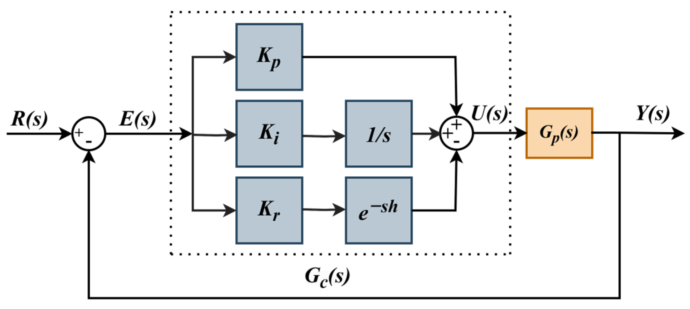
Let us examine the application of the methods described above on the 3rd-order stable time-delay process given in (26) in Figure 1.

$$G_{p_1}(s)={\displaystyle \frac{1}{s(s+1)(s+5)}}{e}^{-0.5s}$$

(26)

Before starting the analysis, the PIR controller time-delay value should be selected as a fixed value. For this example, h = 1 was initially taken. Then, in order to draw SBLs in the planes (K_i, K_r) for a fixed K_p, (K_r, K_p) for a fixed K_i value, and (K_p, K_i) for a fixed K_r value, fixed K_p, fixed K_i, and fixed K_r values should be selected. For this, the controller was initially selected as $G_c(s)=K_p-K_r{e}^{-hs}$, namely the PR controller (K_i = 0). The $K_p-K_r=-D_P(0)/N_p(0)$ RRB line equation defined in Step 1 was updated for the system in (26) and obtained as $K_p-K_r=0$. As n > m, the IRB line will not be formed. The K_p(ω) and K_r(ω) CRB equations are obtained with the help of (24) and (25). 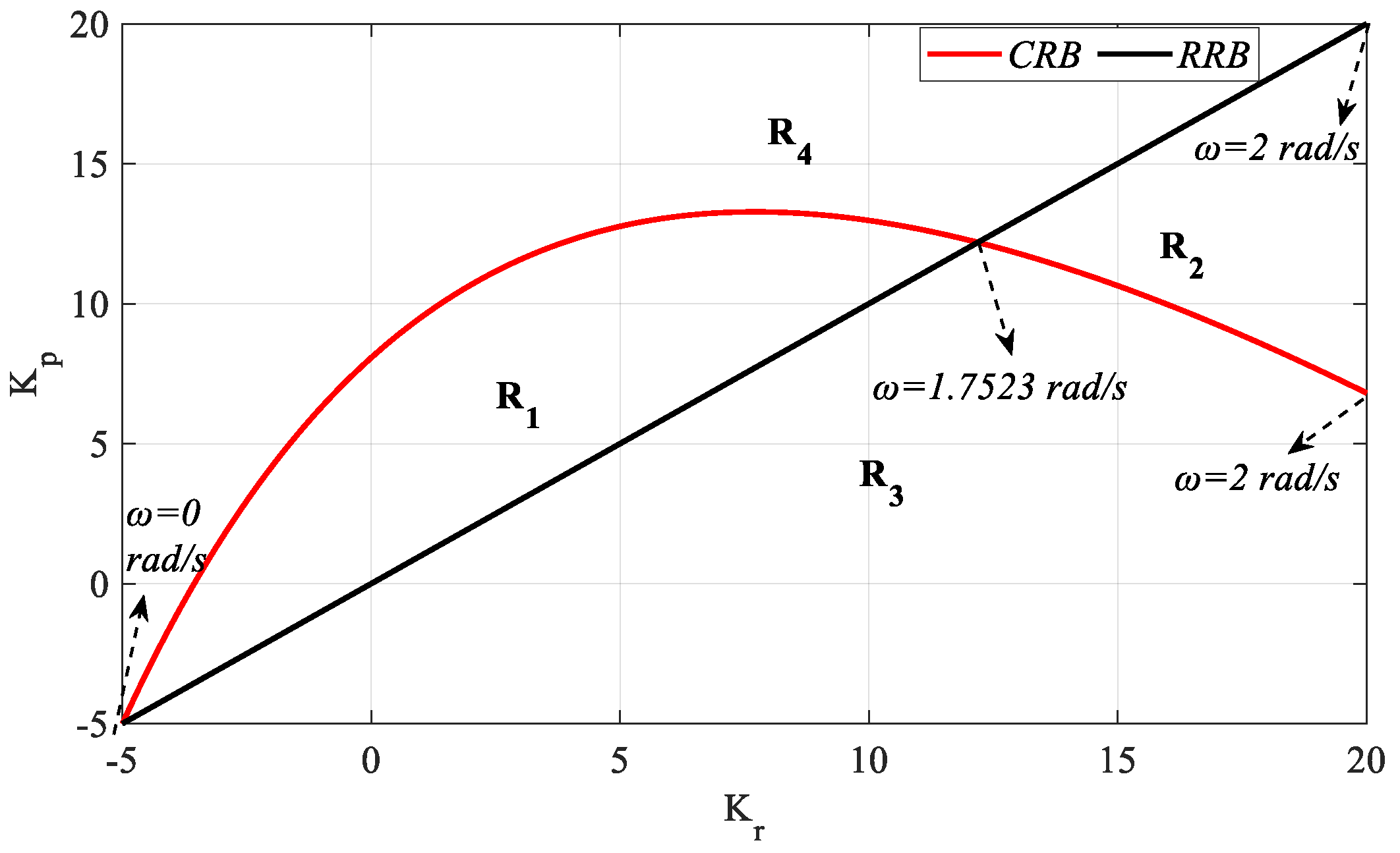Accordingly, the SBL curve was drawn as in Figure 2 with the help of the RRB and CRB equations.

SBL is obtained for the frequency range ω ∈ [0, 2] rad/s as in Figure 2. Here, our aim was to find the entire (K_r, K_p) parameter region that makes the characteristic polynomial in (4) Hurwitz stable. For this purpose, the stability of (4) is examined by selecting the (K_r, K_p) parameter test points from the region bounded by the CRB and RRB lines and the regions outside this region. 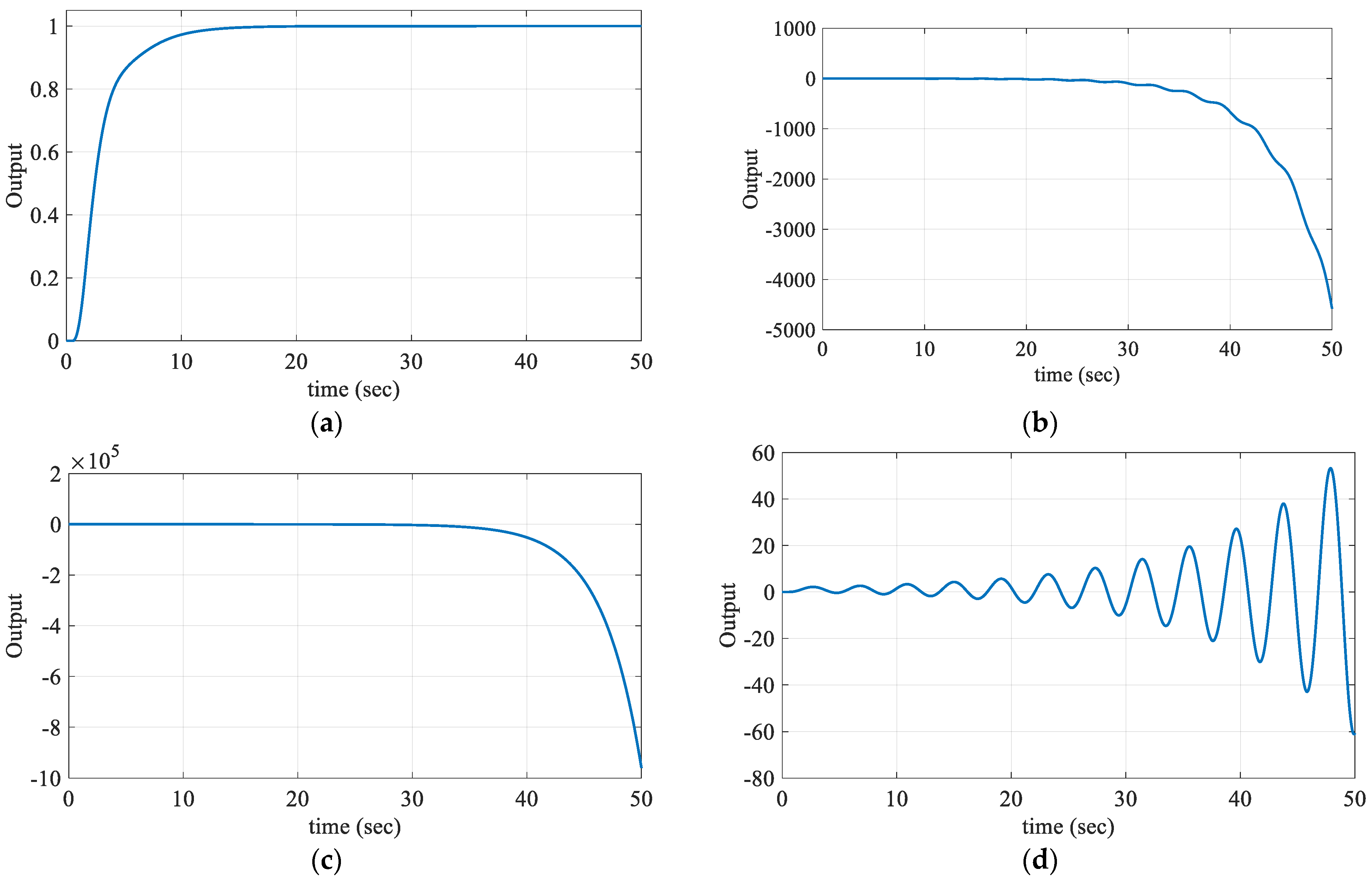The test points (1.60, 3.16), (17.64, 13.22), (8.86, 4.3), and (6.5, 14.98) are selected from the determined R₁, R₂, R₃, and R₄ regions, respectively. The unit step responses obtained according to these test points are given in Figure 3.

As the characteristic equations written in (4) for the test points selected from the R₂, R₃, and R₄ regions have a right half-plane pole, these regions are unstable regions, as seen in Figure 3b–d. The characteristic equation for the test point in the R₁ region has only a left half-plane pole. Therefore, the stable region is the R₁ region that covers the frequency range ω ∈ [0, 1.7523] rad/s, that is, the region bounded by the CRB and RRB lines. 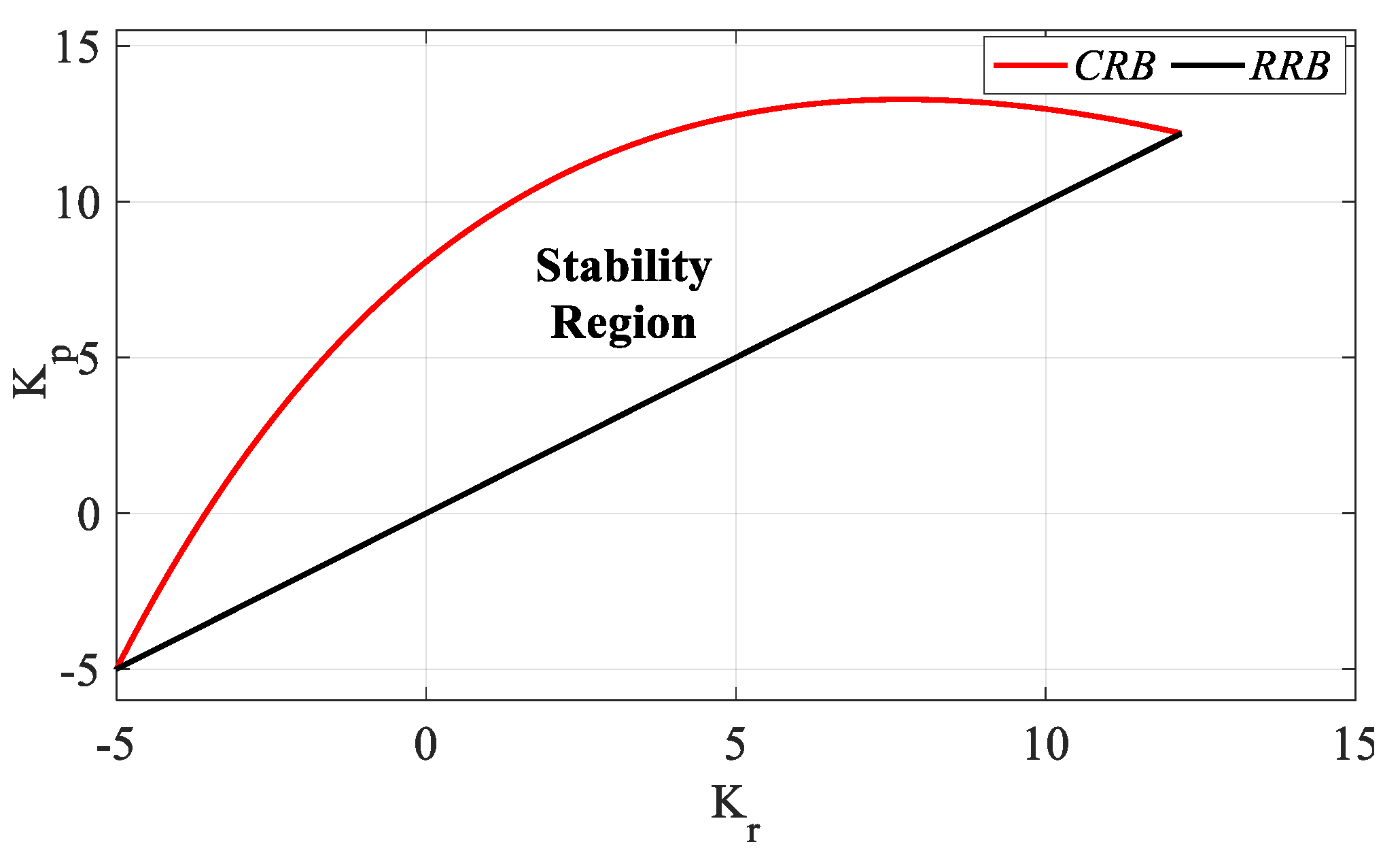Accordingly, the stability region drawn in the (K_r, K_p) plane for the PR controller is given in Figure 4.

When Figure 4 is examined, the K_p and K_r controller parameter ranges that make the system stable are determined as [−5 13.28] and [−5 12.18], respectively. For the controller parameter range K_{r_fixed} = [−2.5:2.5:10], the K_p-K_i SBL graphs are drawn as in Figure 5 with the help of the RRB defined with the K_i = 0 line equation and with the CRB equations calculated with the help of (16) and (17).

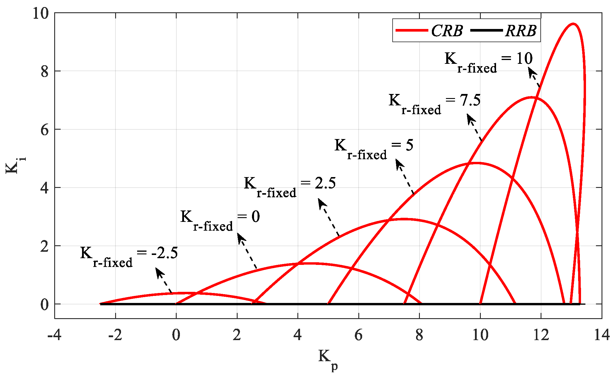
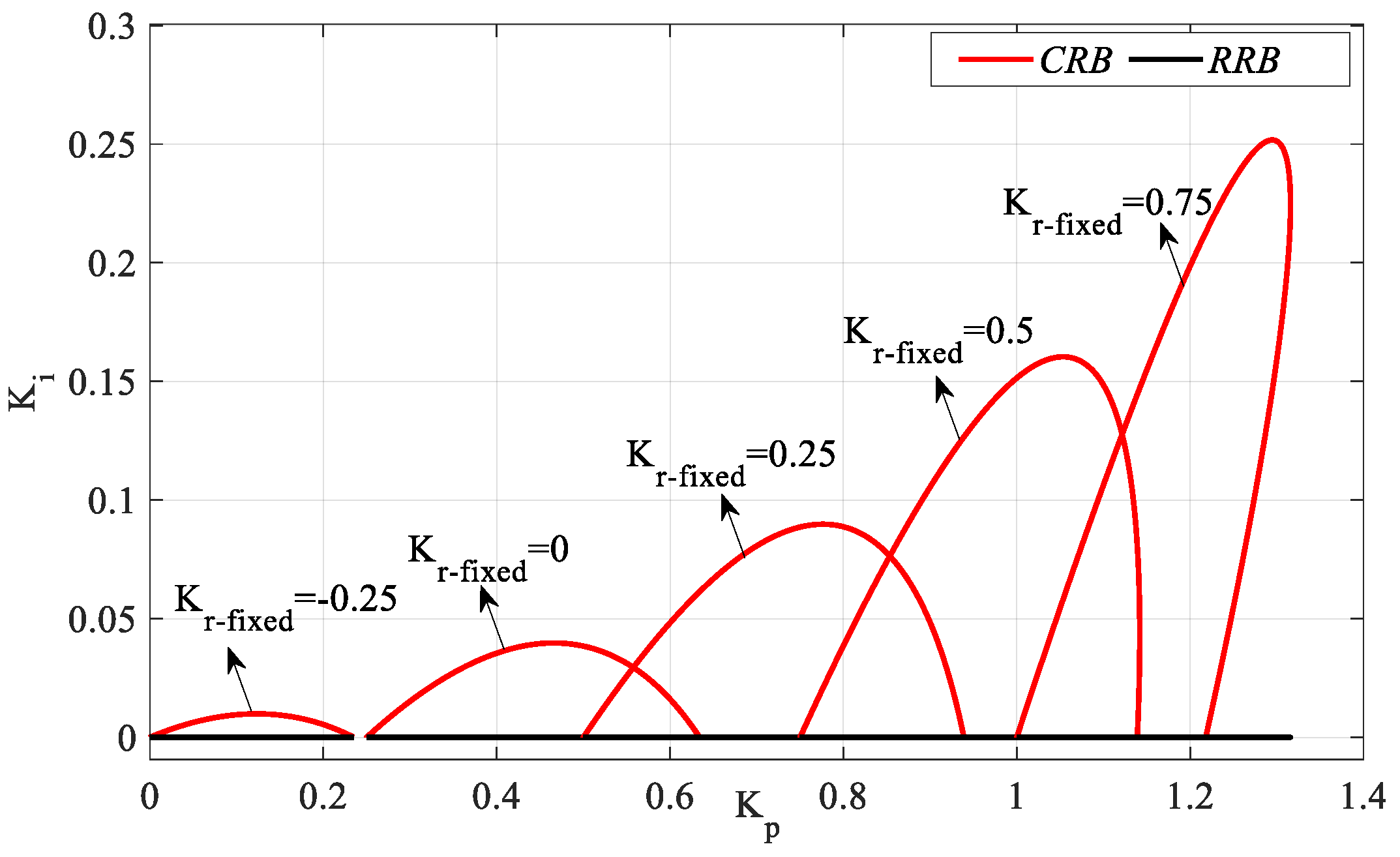
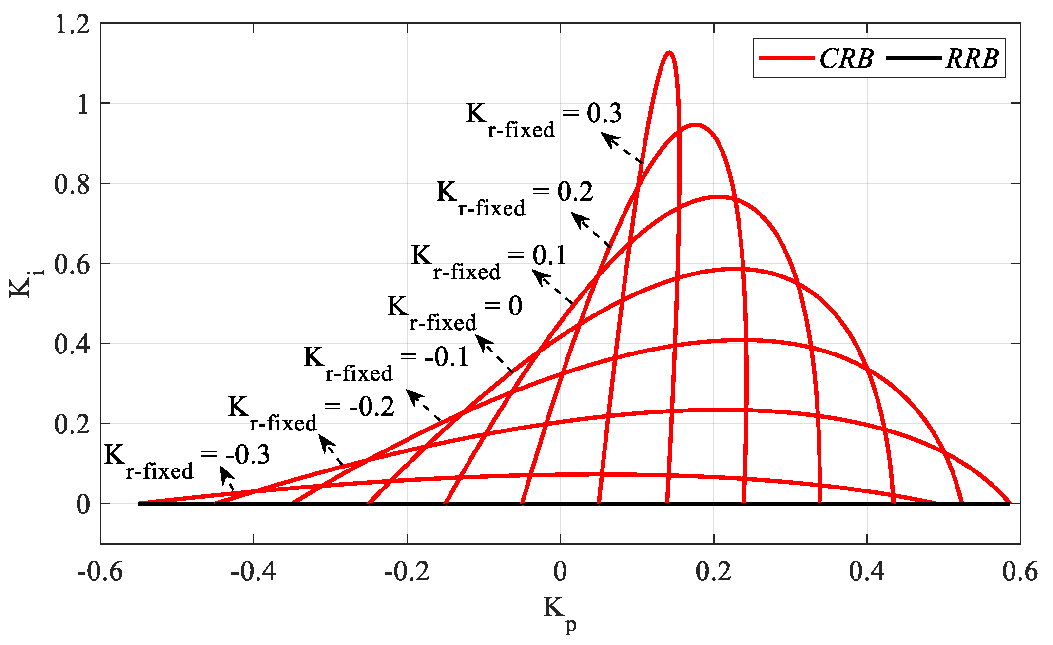
Figure 5 is obtained by plotting the K_p-K_i SBLs in the frequency range ω ∈ [0, ω_max] rad/s for K_{r_fixed} = −2.5, 0, 2.5, 5, 7.5, and 10 values. According to the stability analyses for these K_{r_fixed} values, ω_max values were found to be 0.7846, 1.0749, 1.2782, 1.4355, 1.5636, and 1.6710 rad/s, respectively. It should be noted that, for K_{r_fixed} = 0, the controller will become a PI controller, and the controller time delay h will have no effect on the SBL. It is also concluded that the stability range K_p corresponding to each K_r value in the SBL curve in Figure 4 is the same as the K_p range in the SBL curve drawn for the corresponding K_r value in Figure 5. For example, it is seen in Figure 4 that the K_p range corresponding to K_r = 5 is [5 12.76]. When the K_p-K_i SBL graph in Figure 5 drawn for K_{r_fixed} = 5 is analyzed, it is seen that the stable K_p range is [5 12.76] again. With the same reasoning, as there is no K_p range that makes the system stable for K_r = −5 and K_r = 12 values in Figure 4, these are not plotted in Figure 5.

The K_i controller parameter range will be determined for an SBL selected from the SBL graphs of the system with the PIR controller designed for different K_{r_fixed} values in Figure 5. According to the K_p-K_i SBL graph of the PIR controller designed for K_{r_fixed} = 7.5 selected from Figure 5, it is seen that the K_i controller parameter range that makes the system stable is [0 7.09]. For different K_{i_fixed} values to be selected from the K_i controller parameter range, SBL graphs are obtained with the help of an RRB defined by $K_p-K_r=0$ and a CRB line to be drawn with the help of (19) and (20). 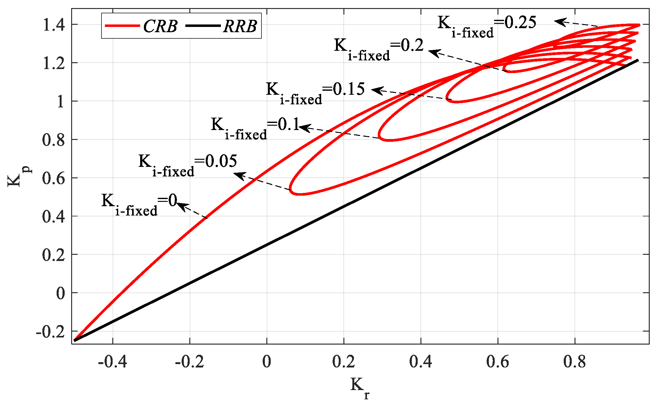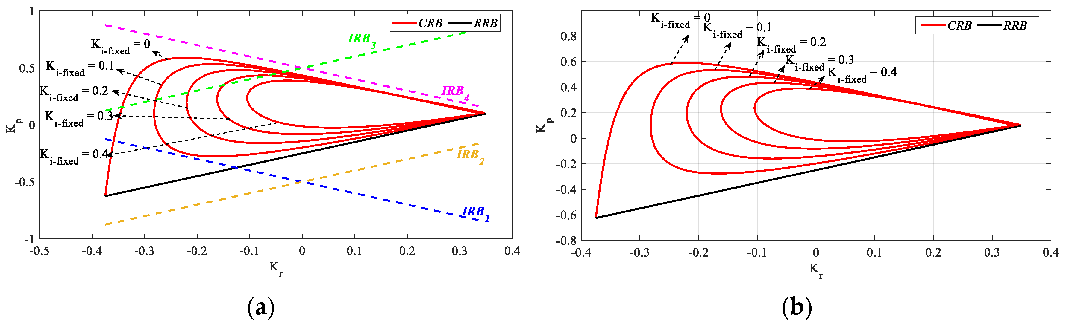SBL curves for the controller parameter range K_{i_fixed} = [0:1:7] are drawn as shown in Figure 6.

Figure 6 was obtained by plotting K_r-K_p SBLs in the frequency range ω ∈ [ω_min, ω_max] rad/s for K_{i_fixed} = 0, 1, 2, 3, 4, 5, 6 and 7. Accordingly, in the stability analyses performed for these K_{i_fixed} values, the frequency ranges that make the system stable are ω ∈ [0, 1.7523], [0.244, 1.73], [0.35, 1.715], [0.432, 1.7], [0.505, 1.665], [0.575, 1.64], [0.641, 1.61] and [0.706, 1.58], respectively. For K_{i_fixed} = 0, the controller will become a PR controller, and the RRB line defined by $K_p-K_r=0$ is the determining factor of the stability boundary only in this case, as can be seen from Figure 6. For K_i ≠ 0, the RRB line is not a determining factor of the stability boundary.

When the K_p-K_i SBL graph for K_{r_fixed} = 7.5 was analyzed in Figure 5, it was seen that, as the value of K_{i_fixed} increases, the K_p controller parameter range that makes the system stable decreases. In Figure 6 of this analysis, it is seen that K_r-K_p SBLs become smaller for increasing K_{i_fixed} values, that is, the controller parameter space that makes the system stable becomes limited.

From the SBL plot for the PR controller in Figure 4, the K_p controller parameter range that makes the system stable was determined as [−5 13.28]. Accordingly, for a K_{p_fixed} selected from the K_p controller parameter space, SBL is generated by an RRB line defined by the equation K_i = 0 and a CRB line to be drawn with the help of (22) and (23). 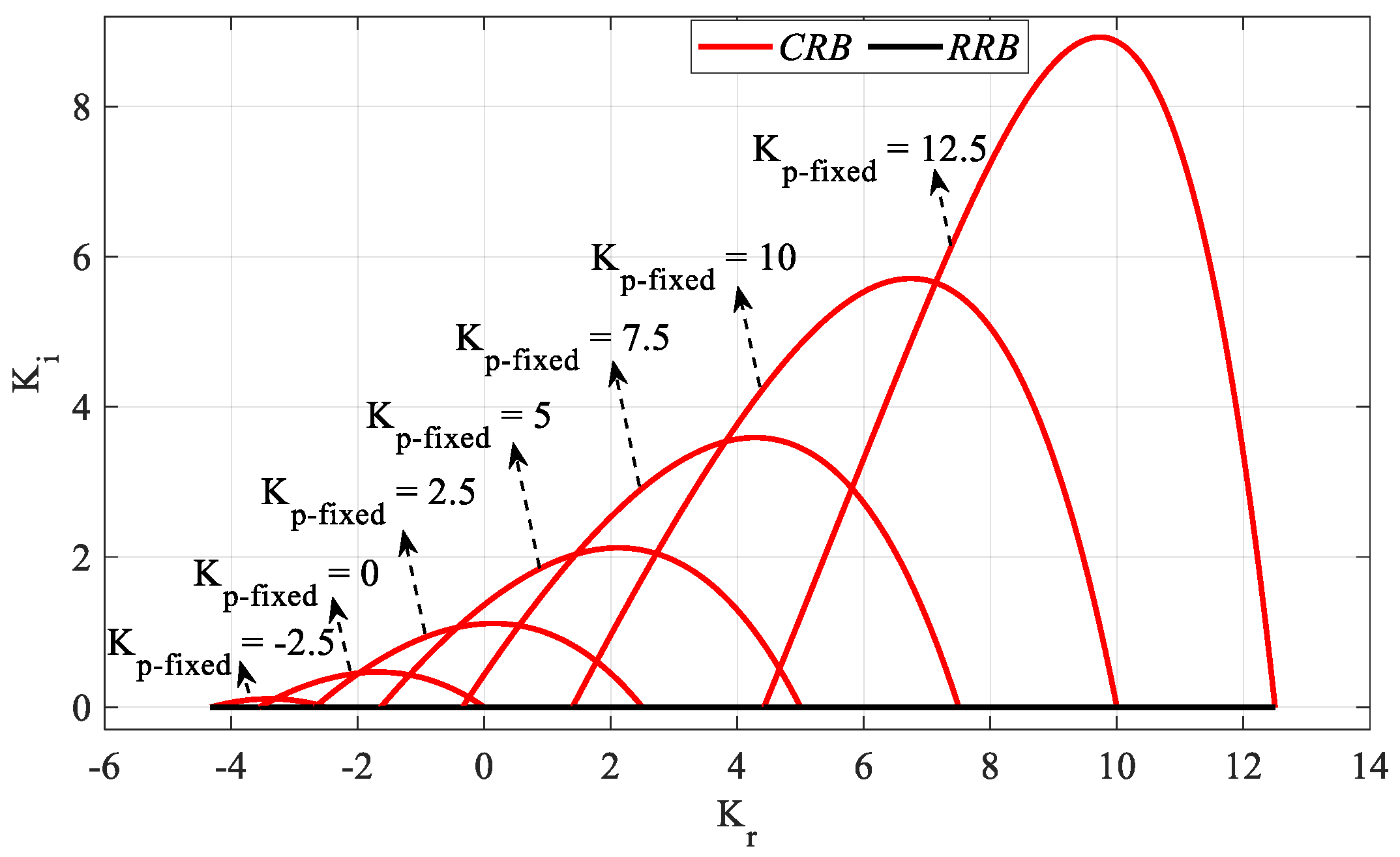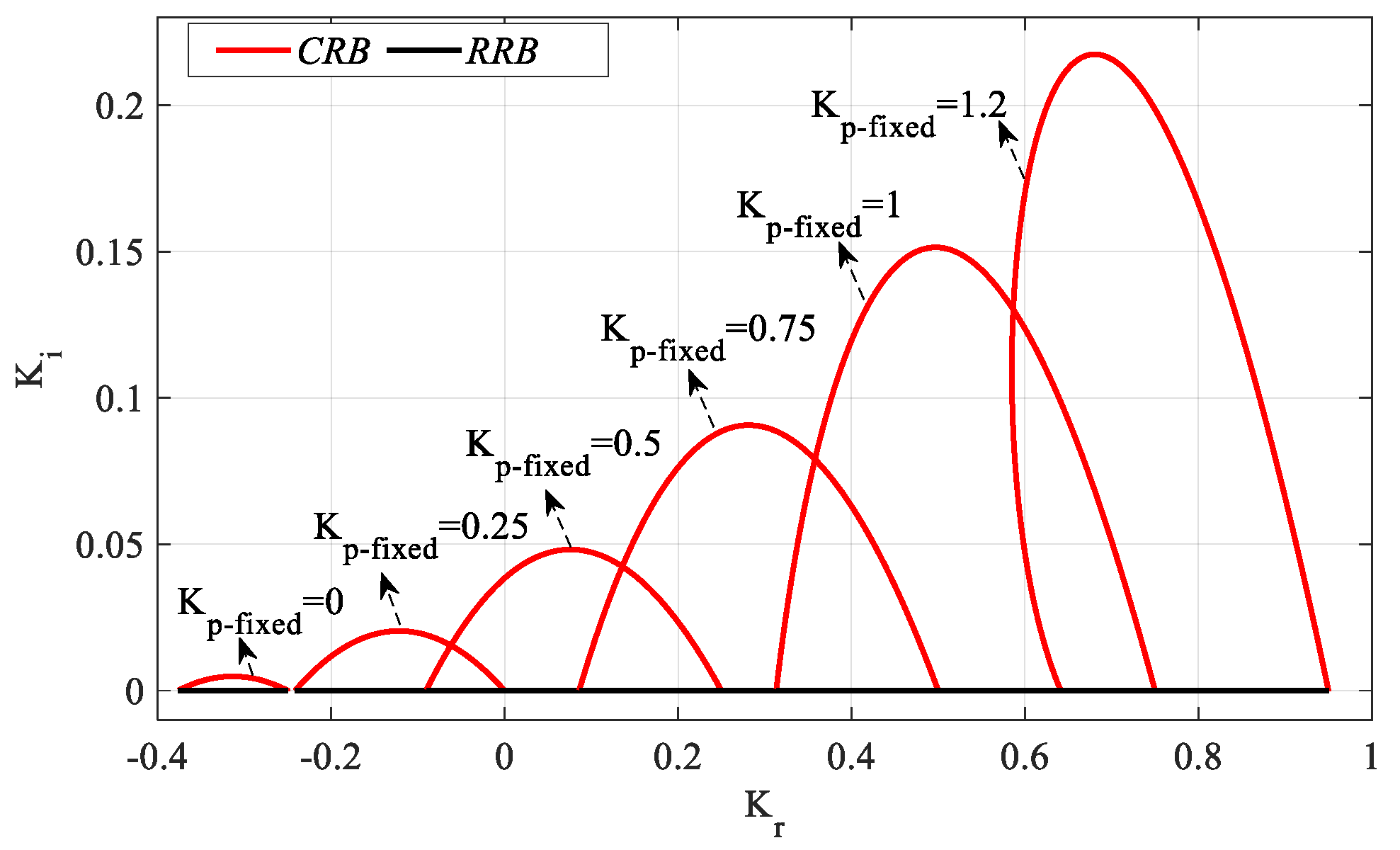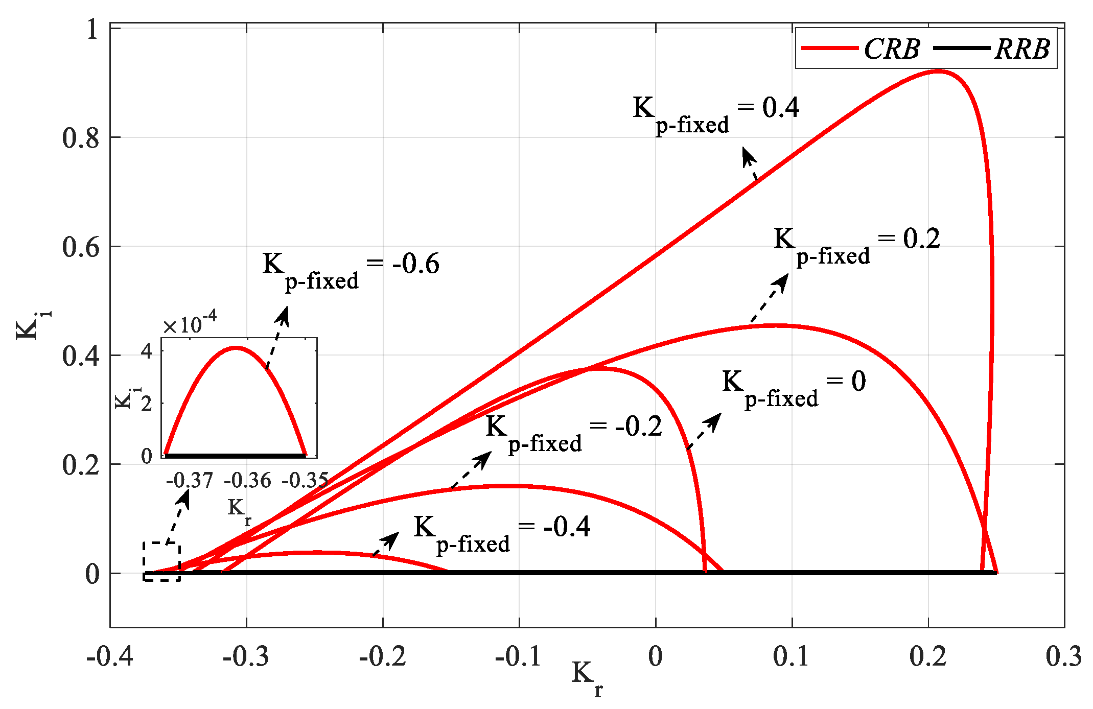Accordingly, SBL plots for the controller parameters of K_{p_fixed} = [−2.5:2.5:12.5] are drawn as shown in Figure 7.

Figure 7 is obtained by plotting K_r-K_i SBLs in the frequency range ω ∈ [0, ω_max] rad/s for K_{p_fixed} = −2.5, 0, 2.5, 5, 7.5, 10, and 12.5 values. According to the stability analyses for these K_{p_fixed} values, ω_max values were found to be 0.4193, 0.6044, 0.7582, 0.901, 1.0415, 1.1953, and 1.4021 rad/s, respectively. It should be noted that, for K_{p_fixed} = 0, the controller will become an IR controller. It is also concluded that the stability range K_r corresponding to each K_p value in the SBL curve in Figure 4 is the same as the K_r range in the SBL curve drawn for the corresponding K_{p_fixed} value in Figure 7. In Figure 4, it is seen that the K_r range corresponding to K_p = 2.5 is [−2.67 2.5]. When the K_r-K_i SBL graph in Figure 7 drawn for K_{p_fixed} = 2.5 is examined, it is seen that the stable K_r range is the same. Therefore, there is no K_r range that makes the system stable for K_p = −5 and K_p = 13.28 values in Figure 4, SBL plots for these values are not made in Figure 7.

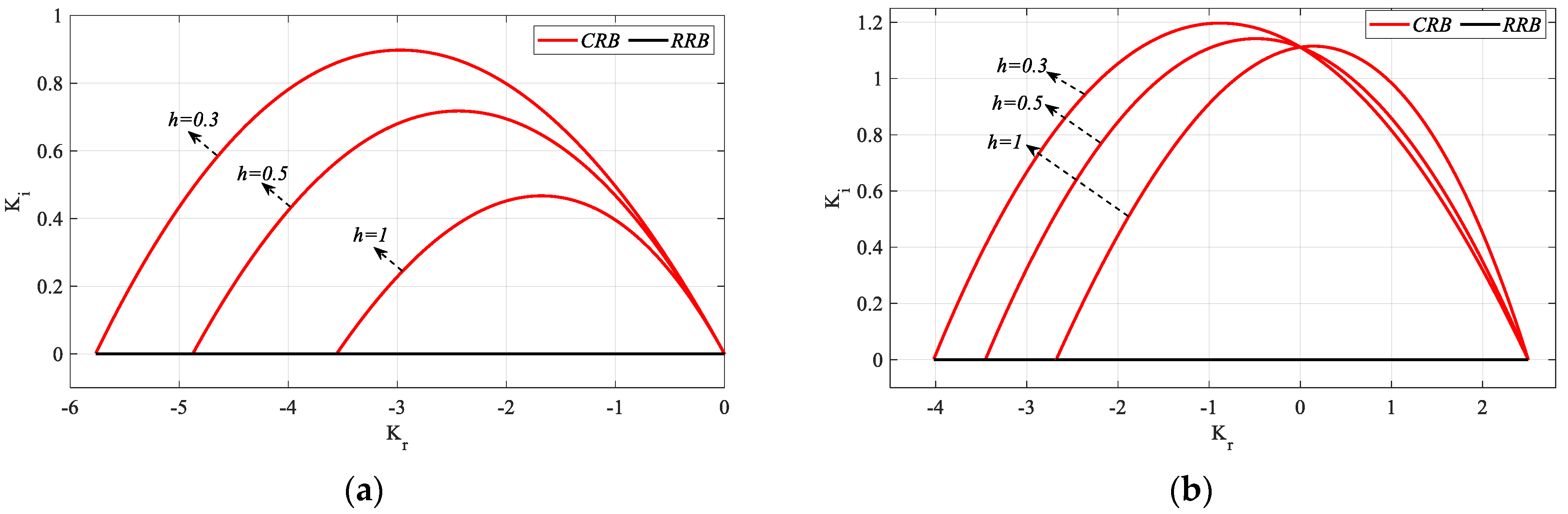
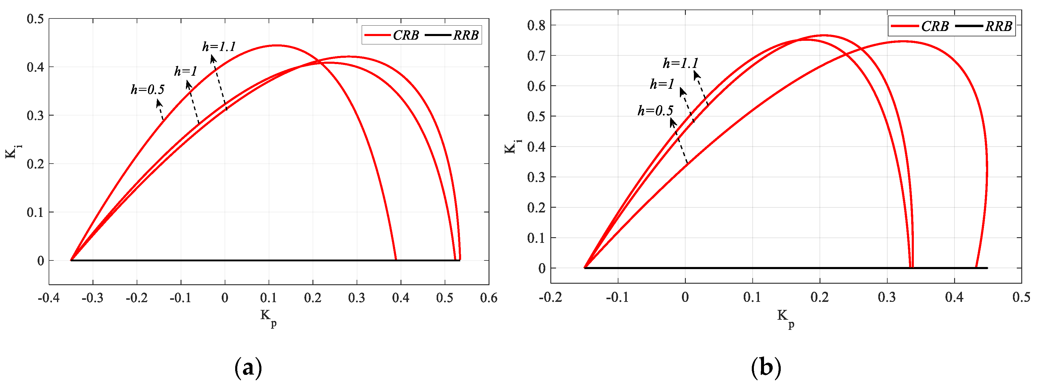
The above analyses were performed for the case where the controller time delay h is 1 s. SBL analyses should be repeated for different values of h to investigate the effect of the controller time delay on the stable controller parameter space. Therefore, three cases where the controller time delay is greater than, equal to, and less than the process time delay are analyzed in this study. The case where the controller time delay is greater than the process time delay is h = 1 as examined above, and the analyses are repeated for cases h = 0.5 (h = $\theta$) and h = 0.3 (h < $\theta$).

The analysis for h = 1 in Figure 2 is repeated for h = 0.3 and h = 0.5, and the frequency ranges that make the system stable are found as ω ∈ [0, 2.3565] rad/s and ω ∈ [0, 2.1386] rad/s, respectively. Accordingly, the K_r and K_p controller parameter ranges that make the system stable for h = 0.3 are found to be [−16.67 47.913] and [−16.67 47.913], respectively, and [−10 26.68] and [−10 27.07] for h = 0.5, respectively. It can be concluded that the stable controller parameter space will expand as the value of h decreases. 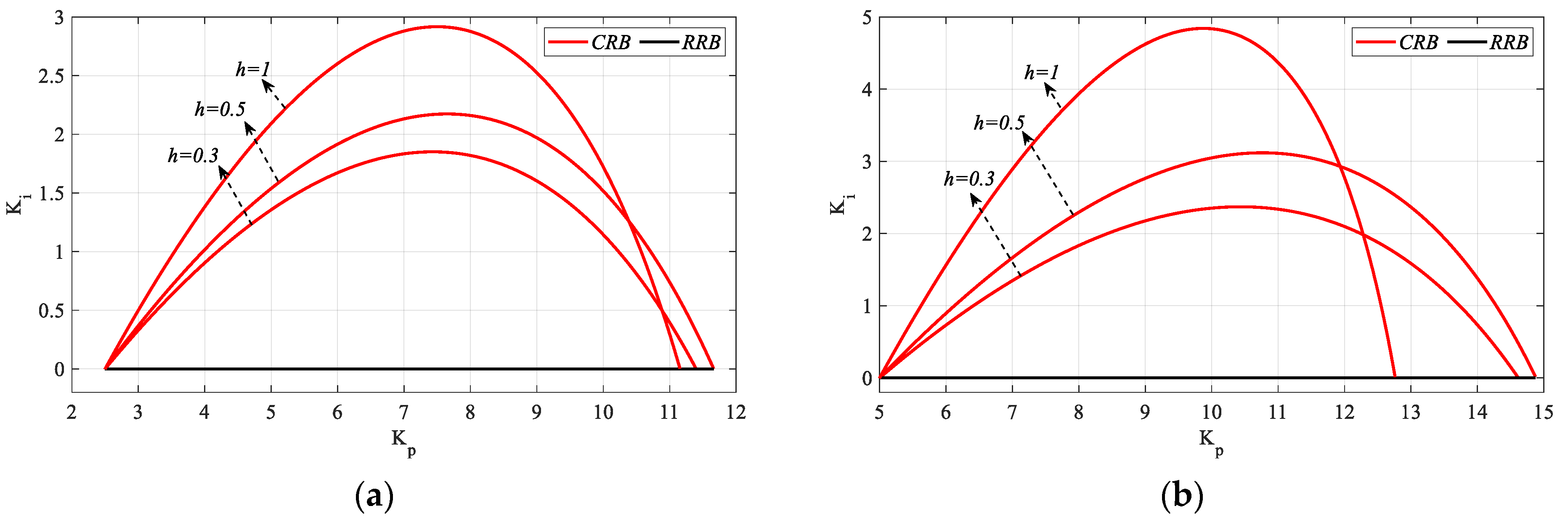Then, K_p-K_i SBL plots for K_{r_fixed} = 2.5 and 5 values selected from the stable controller parameter range are obtained as shown in Figure 8. In Figure 8a, ω_max values for h = 0.3, 0.5 and 1 are 1.1575, 1.2051 and 1.2782 rad/s respectively, and in Figure 8b, ω_max values for h = 0.3, 0.5, and 1 are 1.2359, 1.3239, and 1.4355 rad/s respectively. For K_{r_fixed} = 0, as the controller will become a PI controller, the value of h will have no effect on SBL and the SBL curve will be the same as in Figure 5.

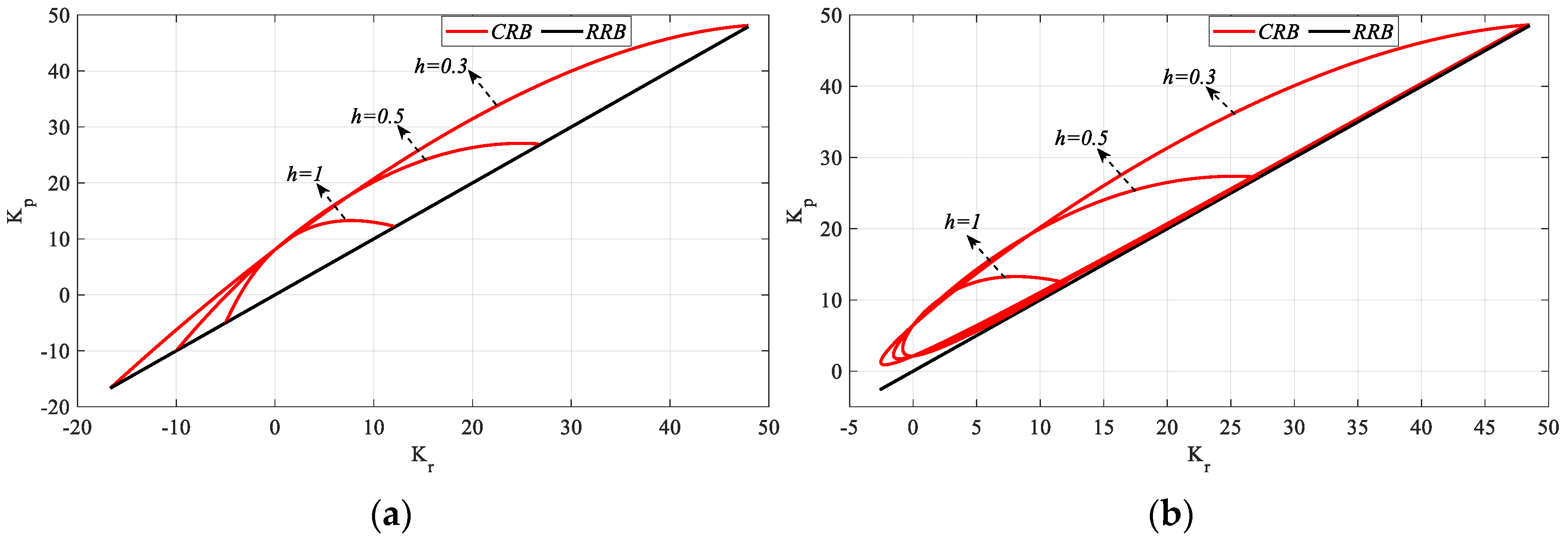
The K_r-K_p SBLs obtained for K_{i_fixed} = 0 and 1 values selected from the range of common stable K_i controller parameters for all h values in Figure 8 are shown in Figure 9.

In Figure 9a, the frequency ranges that make the system stable for h = 0.3, 0.5 and 1 are ω ∈ [0, 2.3565], [0, 2.1386] and [0, 2.1386] rad/s, respectively, while in Figure 9b, ω ∈ [0.2285, 2.35], [0.234, 2.13] and [0.244, 1.73] rad/s are found. Therefore, it can be said that the frequency range that stabilizes the system narrows as the value of h increases. Accordingly, it is seen from Figure 9 that the SBL curves also narrow. Similarly, K_r-K_i SBL graphs were obtained for the K_{p_fixed} = 0 and K_{p_fixed} = 2.5 values selected from the stable K_p controller parameter ranges shown in Figure 8 and Figure 10.

In Figure 10a, the frequency ranges that make the system stable for h = 0.3, 0.5, and 1 are ω ∈ [0, 0.8614], [0, 0.7654] and [0, 0.6044] rad/s, respectively, while in Figure 10b, ω ∈ [0, 0.9303], [0, 0.8665] and [0, 0.7582] rad/s are found, respectively. Similar to the previous analyses, as the value of h increases, the frequency range that makes the system stable narrows. Therefore, it is seen from Figure 10 that the SBL curves narrow as the h value increases.

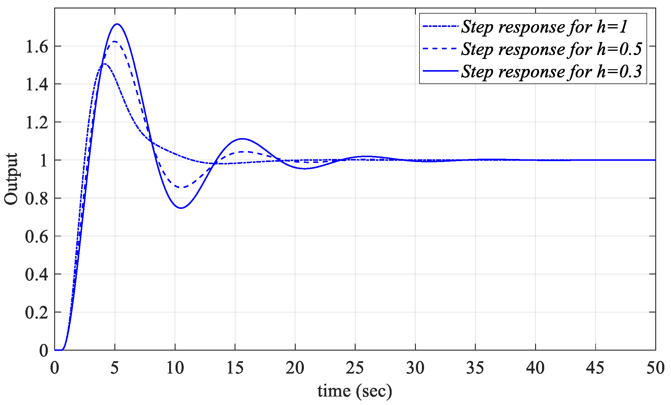
The unit step responses for different K_p, K_i, and K_r values selected from the common regions of the SBL curves obtained for h = 0.3, 0.5, and 1 in respective Figure 8a, Figure 9b and Figure 10b were analyzed. 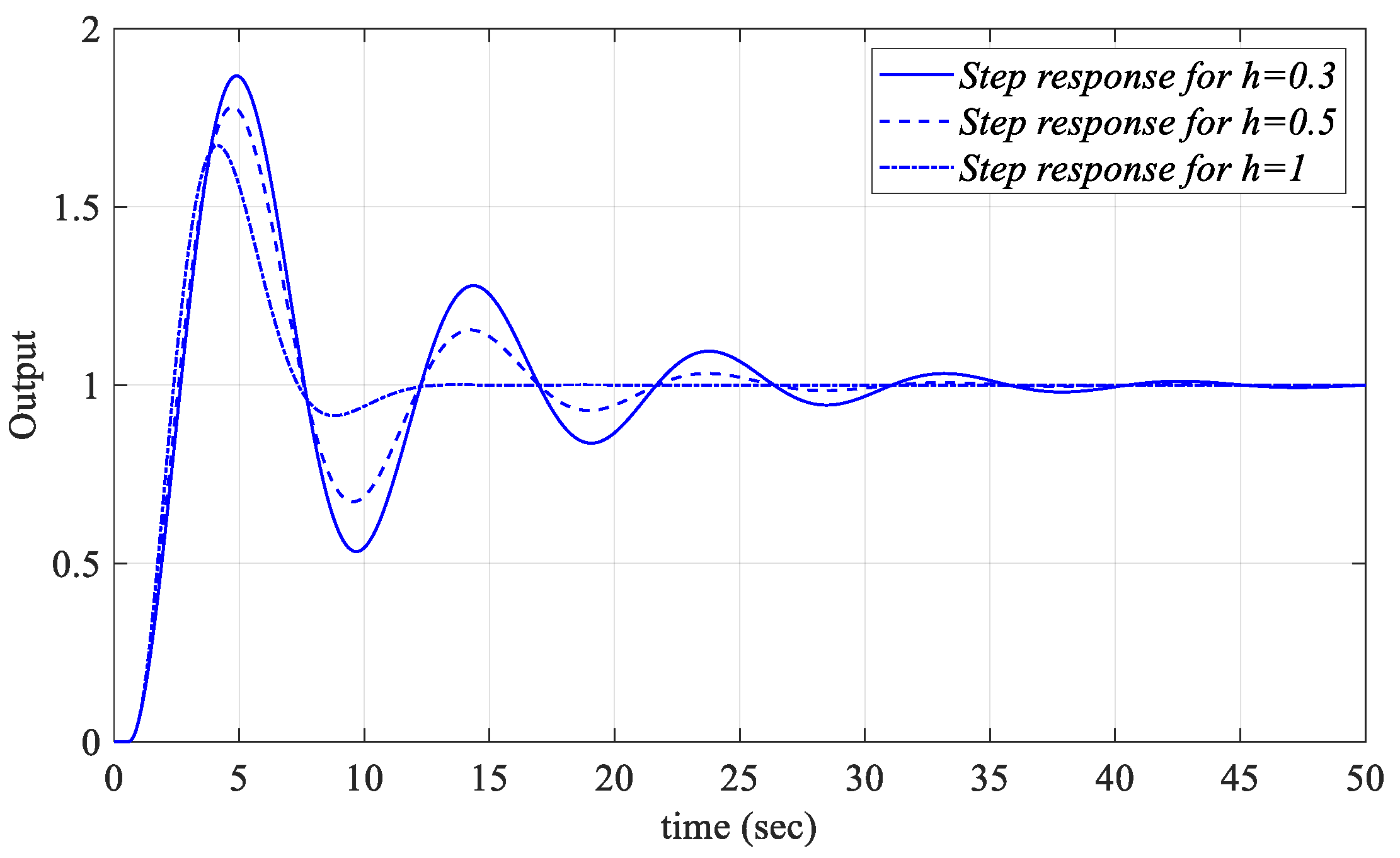In this context, for K_{r_fixed} = 2.5, PIR controllers were designed for the K_p = 5.74 and K_i = 0.76 values selected from the common region of the K_p-K_i SBL curves in Figure 8a and the unit step responses obtained by implementing these PIR controllers to Figure 1 are shown in Figure 11. 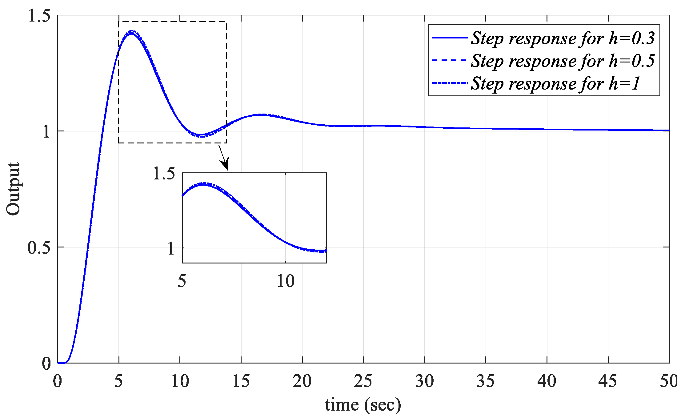The unit step responses for the K_r = 2.256 and K_p = 5.9 controller parameter values selected from the K_r-K_p SBL plot in Figure 9b for K_{i_fixed} = 1 and for different h values are shown in Figure 12. Similarly, controller parameter values of K_r = −0.13 and K_i = 0.18 are selected from the K_r-K_i SBL plot in Figure 10b, which was obtained for K_{p_fixed} = 2.5 and unit step responses for h = 0.3, 0.5, and 1 are presented in Figure 13.

When Figure 11, Figure 12 and Figure 13 are analyzed, it can be said that the PIR controllers designed for different values of h and different values of K_p, K_i, and K_r selected from the stable controller parameter regions will control the closed-loop system in Figure 1 successfully.

5.2. Example 2

The unstable first order plus time delay (UFOPTD) process given in (27) was selected from the literature [36,49,50].

$$G_{p_2}(s)={\displaystyle \frac{4}{4s-1}}{e}^{-2s}$$

(27)

Initially, h = 1 was taken at the beginning. Then, to draw SBLs for a fixed K_p value in the (K_i, K_r) plane, for a fixed K_i value in the (K_r, K_p) plane and for a fixed K_r value in the (K_p, K_i) plane, fixed K_p, fixed K_i and fixed K_r values must be respectively selected in the planes. For this purpose, the controller was initially selected as a PR controller (K_i = 0).

The $K_p-K_r=-D_P(0)/N_p(0)$ RRB equation defined in Step 1 is updated for the system in (27) and obtained as $K_p-K_r=0.25$. As n > m, there will be no IRB line. The CRB equations K_p(ω) and K_r(ω)are obtained from (24) and (25), respectively. Accordingly, with the help of the RRB and CRB equations, the SBL curve is drawn as shown in Figure 14.

As can be seen from Figure 14, the stability region for the PR controller is found as the intersection region of the RRB and CRB lines covering the frequency range ω ∈ [0, 1.7523] rad/s. Accordingly, the K_p and K_r controller parameter ranges that make the system stable are determined as [−0.25 1.22] and [−0.5 0.93], respectively. SBL graphs for the controller parameter range K_{r_fixed} = [−0.25:0.25:0.75] are drawn as shown in Figure 15 with the RRB defined by the line equation K_i = 0 and the CRB equations calculated by (16) and (17).

Figure 15 was obtained by plotting the K_p-K_i SBLs in the frequency range ω ∈ [0, ω_max] rad/s for K_{r_fixed} = −0.25, 0, 0.25, 0.5, and 0.75. According to the stability analyses for these K_{r_fixed} values, ω_max values were found to be 0.4043, 0.5828, 0.7291, 0.8627, and 0.9923 rad/s, respectively. The K_i controller parameter range will be determined for an SBL selected from the SBL curves of the system with a PIR controller designed for different K_{r_fixed} values in Figure 15. Accordingly, according to the SBL graph of the PIR controller designed for K_{r_fixed} = 0.75, the K_i controller parameter range that makes the system stable is [0 0.25]. For different K_{i_fixed} values to be selected from the K_i controller parameter range, SBL graphs are obtained with the help of an RRB defined by $K_p-K_r=0.25$ and a CRB line to be drawn with the help of (19) and (20). Accordingly, SBL plots for the controller parameter range K_{i_fixed} = [0:0.05:0.25] are drawn as shown in Figure 16.

Figure 16 is obtained by plotting K_r-K_p SBLs in the frequency range ω ∈ [ω_min, ω_max] rad/s for K_{i_fixed} = 0, 0.05, 0.1, 0.15, 0.2, and 0.25. For these K_{i_fixed} values, the frequency ranges that make the system stable are ω ∈ [0, 1.0894], [0.1908, 1.068], [0.276, 1.036], [0.347, 1.009], [0.414, 0.975], and [0.482, 0.932], respectively. It is seen that the stable K_r-K_p controller parameter region becomes smaller as the value of K_{i_fixed} increases. In addition, the RRB line defined by the equation of $K_p-K_r=0.25$ is the determining factor of the stability boundary only in the case where K_{i_fixed} = 0, as seen in Figure 16.

From the SBL curve for the PR controller in Figure 14, the K_p controller parameter range that makes the system stable was determined as [−0.25 1.22]. Accordingly, for a K_{p_fixed} selected from the K_p controller parameter space, SBL is generated by an RRB line defined by the equation K_i = 0 and a CRB line to be drawn with the help of (22) and (23). Accordingly, SBL curves for the controller parameter range K_{p_fixed} = [0:0.25:1.2] are drawn as shown in Figure 17.

Figure 17 was obtained by plotting K_r-K_i SBLs in the frequency range ω ∈ [0, ω_max] rad/s for K_{p_fixed} = 0, 0.25, 0.5, 0.75, 1, and 1.2. In the stability analyses for these K_{p_fixed} values, ω_max values were found to be 0.2816, 0.4113, 0.5236, 0.6353, 0.7637, and 0.9359 rad/s, respectively. It is seen that the stable K_r-K_i controller parameter region increases as the value of K_{p_fixed} increases. The above analyses were performed for h = 1, and the analyses were repeated to reflect the effect of different values of h on SBL. In this regard, the cases of h > $\theta$, h =$\theta$, and h < $\theta$ are examined. Although the case of h < $\theta$ is h = 1 as examined above, the analyses are repeated for the cases of h = 2 (h = $\theta$) and h = 2.2 (h < $\theta$).

The analysis for h = 1 in Figure 14 was repeated for h = 2 and h = 2.2, and the frequency ranges that make the system stable were found to be ω ∈ [0, 9015] rad/s and [0, 0.8721] rad/s, respectively. Accordingly, the K_r and K_p parameter ranges that stabilize the system for h = 2 are [−0.25 0.46] and [0 0.785], respectively, and for h = 2.2 are [−0.17 0.42] and [0.024 0.75], respectively. It can be concluded that, as the value of h increases, the stable PR controller parameter region narrows. 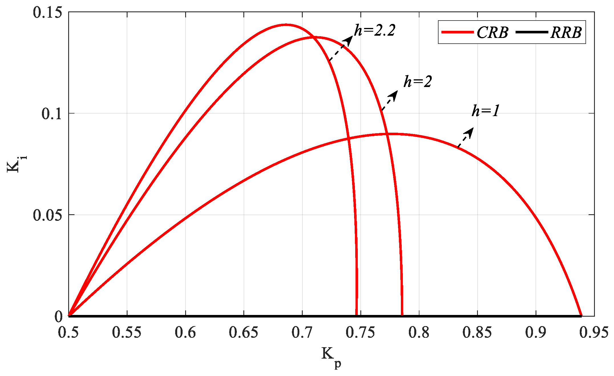For K_{r_fixed} = 2.5 selected from the stable K_r controller parameter range, K_p-K_i SBL curves are obtained as shown in Figure 18. In Figure 18, ω_max values for h = 1, 2, and 2.2 are found to be 0.7291, 0.7853, and 0.7835 rad/s, respectively. It is seen that, as h increases, the stable K_p controller parameter region narrows, and the stable K_i controller parameter region expands. Moreover, as the controller will become a PI controller for K_r = 0, the value of h will have no effect on SBL, and the SBL curve will be the same as in Figure 14.

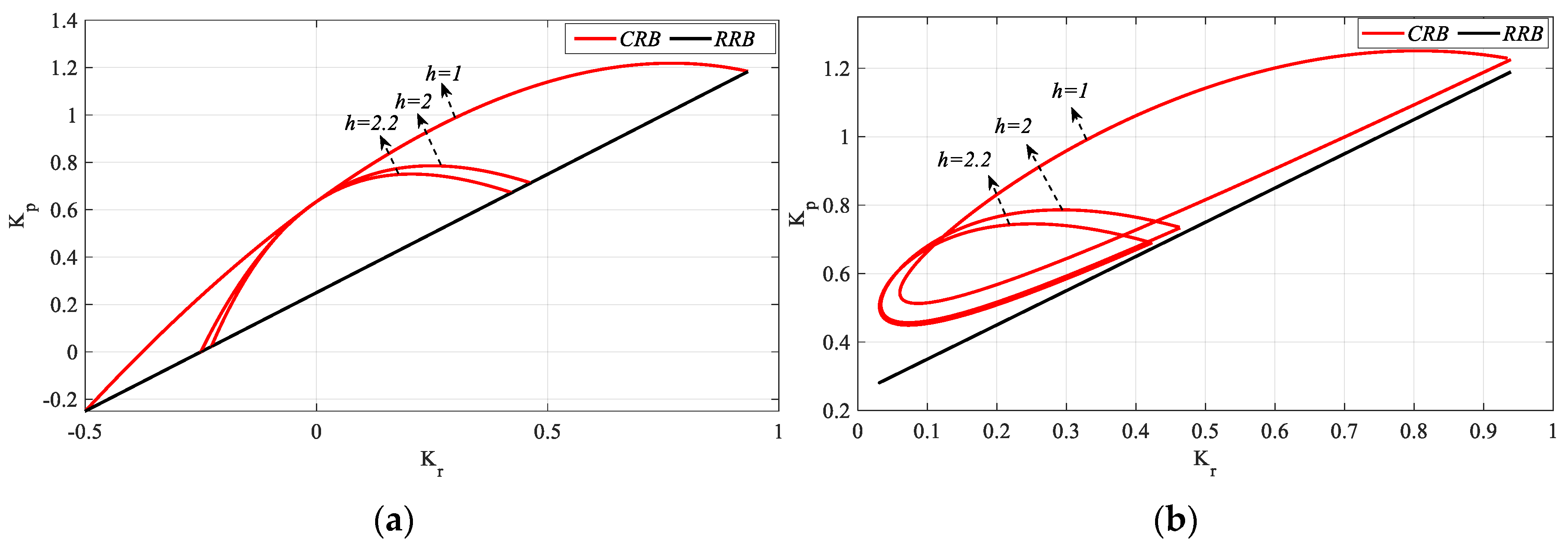
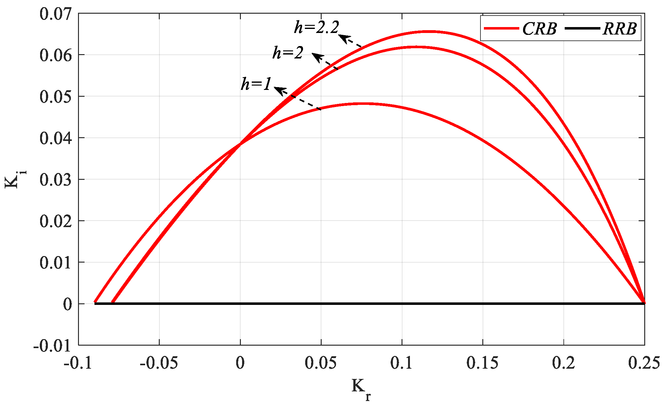
As demonstrated in Figure 18, the SBL curves obtained for h = 1, 2, and 2.2 were analyzed, and K_{i_fixed} = 0 and 0.05 values were selected considering the common stable K_i controller parameter ranges and K_r-K_p SBL graphs for these K_{i_fixed} values, as illustrated in Figure 19.

As demonstrated in Figure 19a, the frequency ranges that stabilize the system for h = 1, 2, and 2.2 are ω ∈ [0, 1.0894], [0, 0.9015], and [0, 0.8721] rad/s, respectively. Similarly, Figure 19b illustrates the corresponding frequency ranges for ω ∈ [0.1908, 1.068], [0.193, 0.879], and [0.193, 0.85] rad/s. Therefore, it can be said that the frequency range that stabilizes the system narrows as the value of h increases. Accordingly, it is seen from Figure 19 that the SBL curves also narrow. In Figure 19a, when K_{i_fixed} = 0, the controller becomes a PR controller. The RRB line, defined by the equation $K_p-K_r=0.25$, is thus a determining factor for the stability boundary. In Figure 19b, however, the RRB line is not a determining factor of the stability boundary; it is only shown as an approximate boundary line for the purpose of enhancing the comprehensibility of the SBL representation. A similar representation is employed for K_r-K_i SBL plots for K_{p_fixed} = 0.5, a parameter that is selected from the stable K_p controller parameter range (see Figure 20).

In Figure 20, the frequency ranges ω ∈ [0, 0.5236], [0, 0.4884], and [0, 0.4822] rad/s are found for h = 1, 2, and 2.2, respectively. It is seen that, as the h value increases, the K_r range that makes the system stable remains almost the same, whereas the stable K_i parameter space increases. For K_{p_fixed} = 0, the controller becomes an IR controller. However, if the SBLs obtained for h = 2 and 2.2 in Figure 19a are analyzed, it is seen that there is no stable K_r controller parameter range corresponding to K_p = 0. From this, it can be concluded that an IR controller that makes the system stable at h = 2 and 2.2 cannot be designed for the G_p2 process.

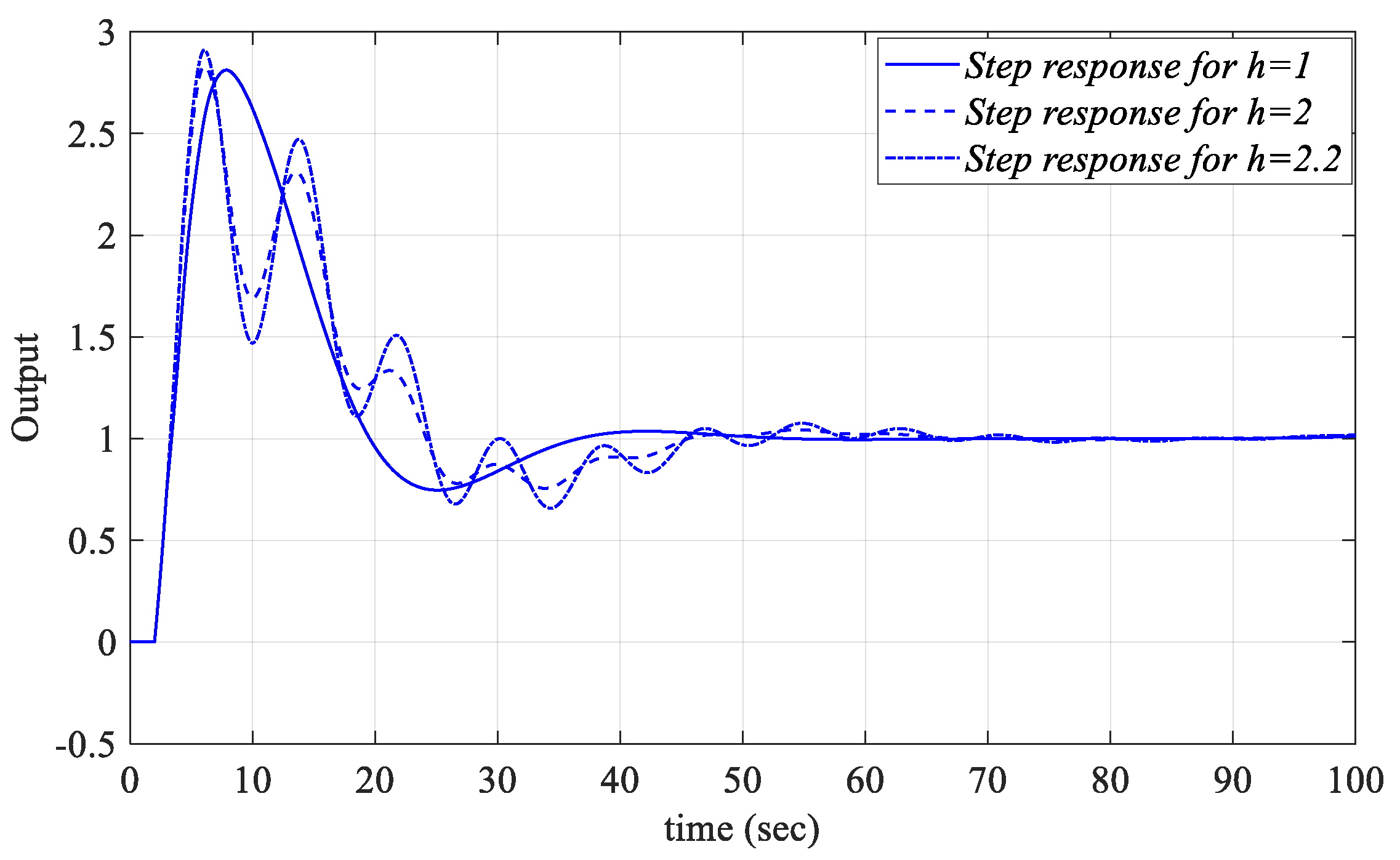
The unit step responses for K_p, K_i, and K_r values selected from the common stability regions of the SBL curves obtained for h = 1, 2, and 2.2 in the respective Figure 18, Figure 19b and Figure 20 are analyzed. The PIR controllers designed according to these parameters are expected to control the G_p2 model in Figure 1 stably for the cases h = 1, 2, and 2.2. For K_{r_fixed} = 0.25, K_p = 0.6598, and K_i = 0.0214, values were selected from the common region of the K_p-K_i SBL graphs drawn for h = 1, 2 and 2.2 in Figure 18, and the PIR controllers designed for these values were applied to Figure 1. 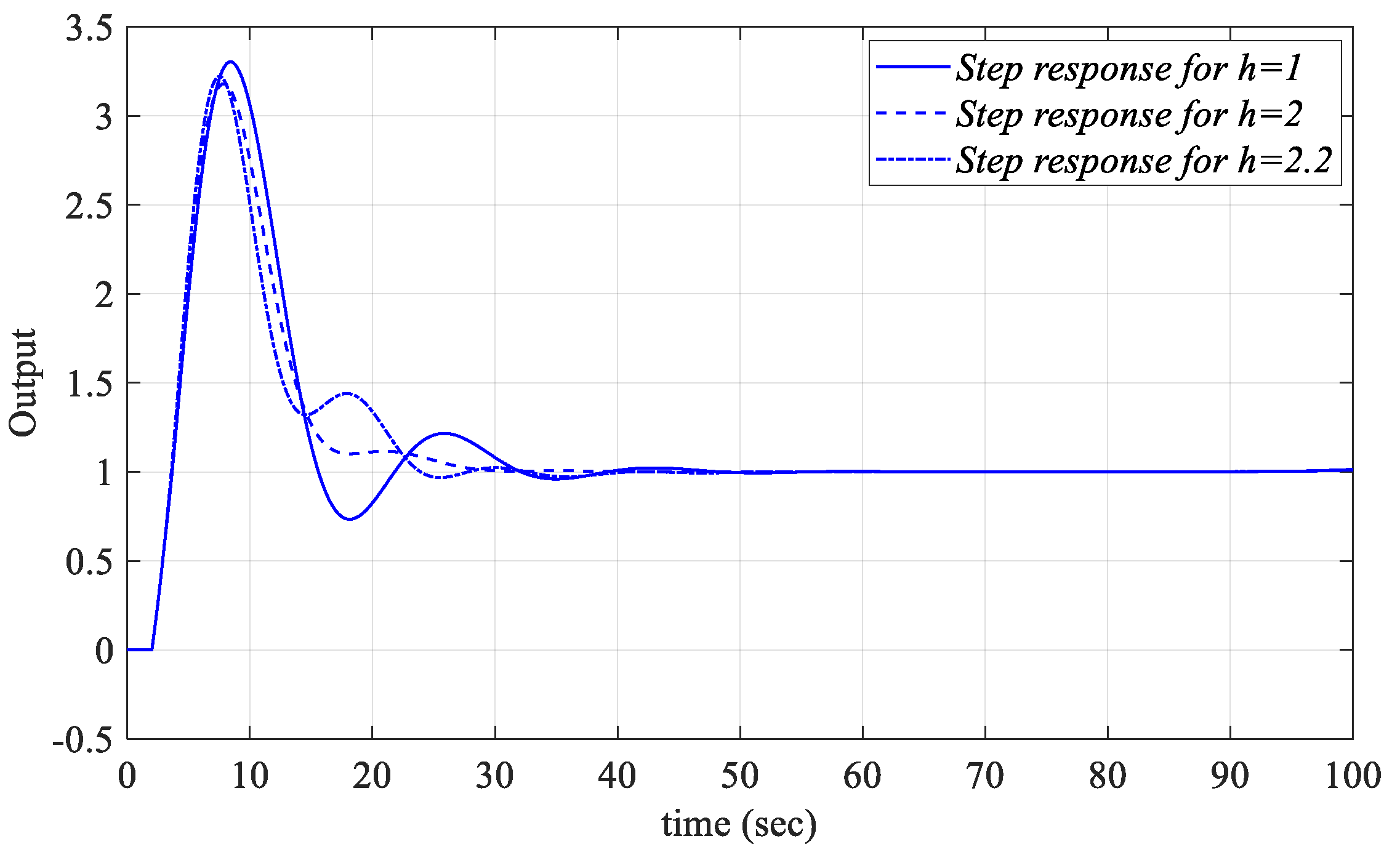The unit step responses were obtained as shown in Figure 21. 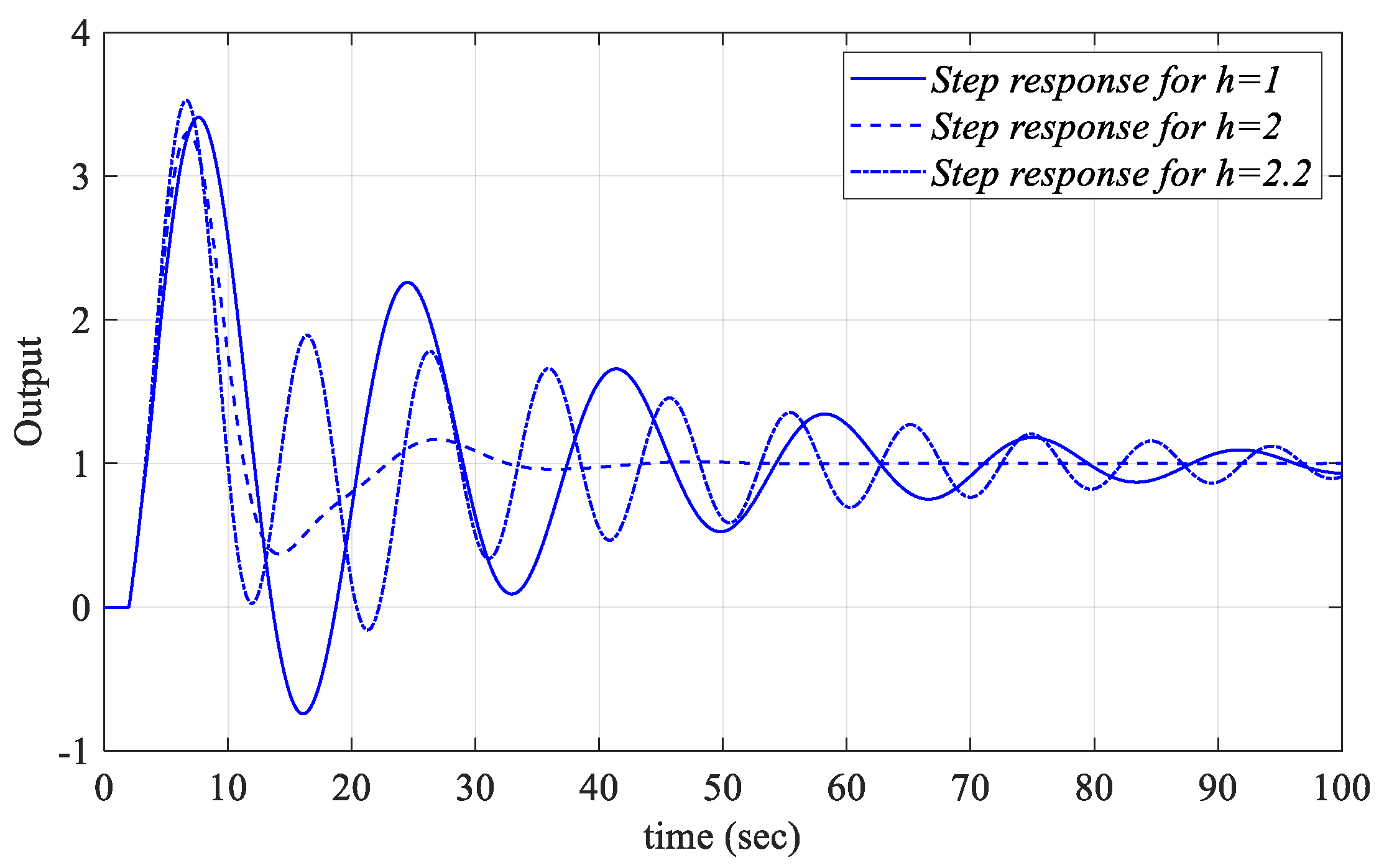For K_{i_fixed} = 0.05, PIR controllers were designed for the K_p = 0.5984 and K_r = 0.16 controller parameter values selected from the K_r-K_p SBL plot in Figure 19b and unit step responses for different h values are shown in Figure 22. In a similar manner, K_r = 0.0187 and K_i = 0.073 controller parameter values are selected from the K_r-K_i SBL graph in Figure 20, obtained for K_{p_fixed} = 0.5. Unit step responses for h = 1, 2, and 2.2 are presented as in Figure 23.

When the unit step responses in Figure 21, Figure 22 and Figure 23 are examined, it is seen that the PIR controllers, designed for the controller parameters selected from the common stability regions of the SBL curves drawn for the cases h = 1, 2 and 2.2, control the G_p2 unstable time-delay process in Figure 1 in a stable manner.

5.3. Example 3

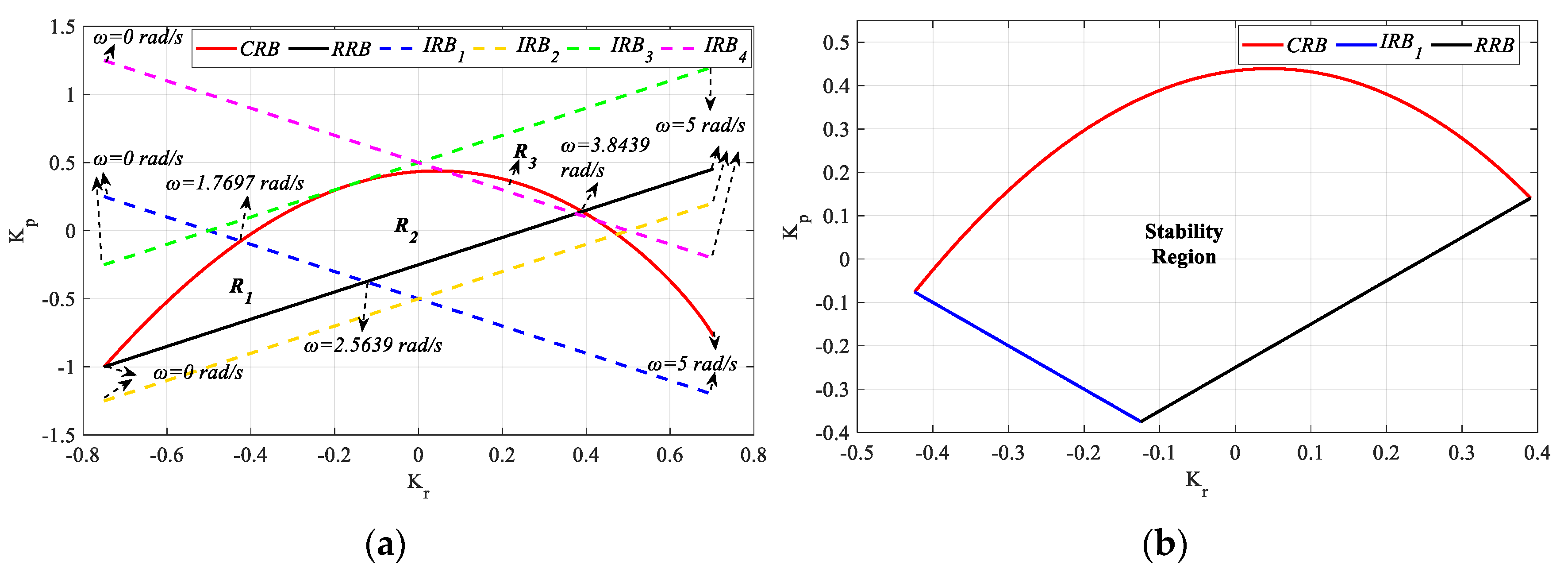
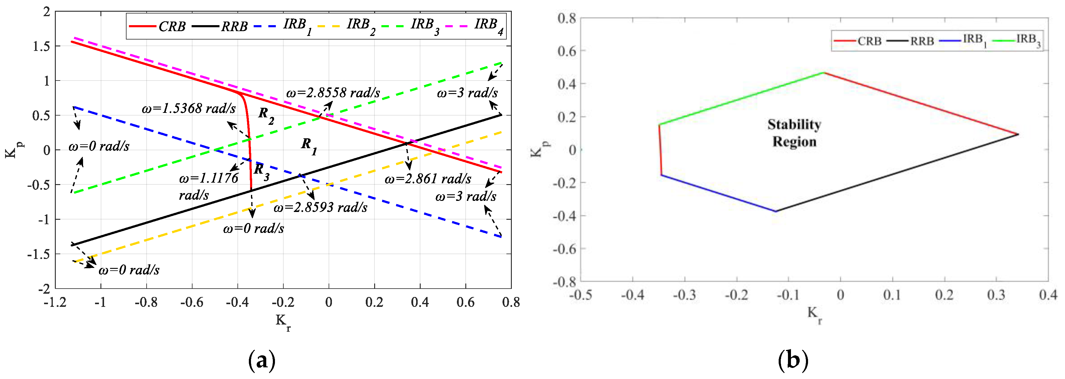
As IRB lines are only observed in processes with equal orders of numerator and denominator polynomials, (28) is chosen for analysis. The FOPTD G_p3(s) process is analyzed through Figure 1.

$$G_{p3}(s)={\displaystyle \frac{2s+4}{s+1}}{e}^{-s}$$

(28)

Before starting the analysis, the PR controller time-delay value is taken as h = 1. The defined $K_p-K_r=-D_P(0)/N_p(0)$ RRB equation is updated for the process in (28) and obtained as $K_p-K_r=-0.25$. According to the IRB rule defined in (11), as n = m, IRB lines are expected to be formed, and one or some of these lines are expected to play a role in determining the stability region. Accordingly, this is achieved with the help of the IRB₁, IRB₂, IRB₃, and IRB₄ equations, which can be seen, respectively, as follows:

$$\begin{array}{l}IR{B}_1\to K_p=-K_r-0.5, IR{B}_2\to K_p=K_r-0.5\\ IR{B}_3\to K_p=K_r+0.5, IR{B}_4\to K_p=-K_r+0.5\end{array}$$

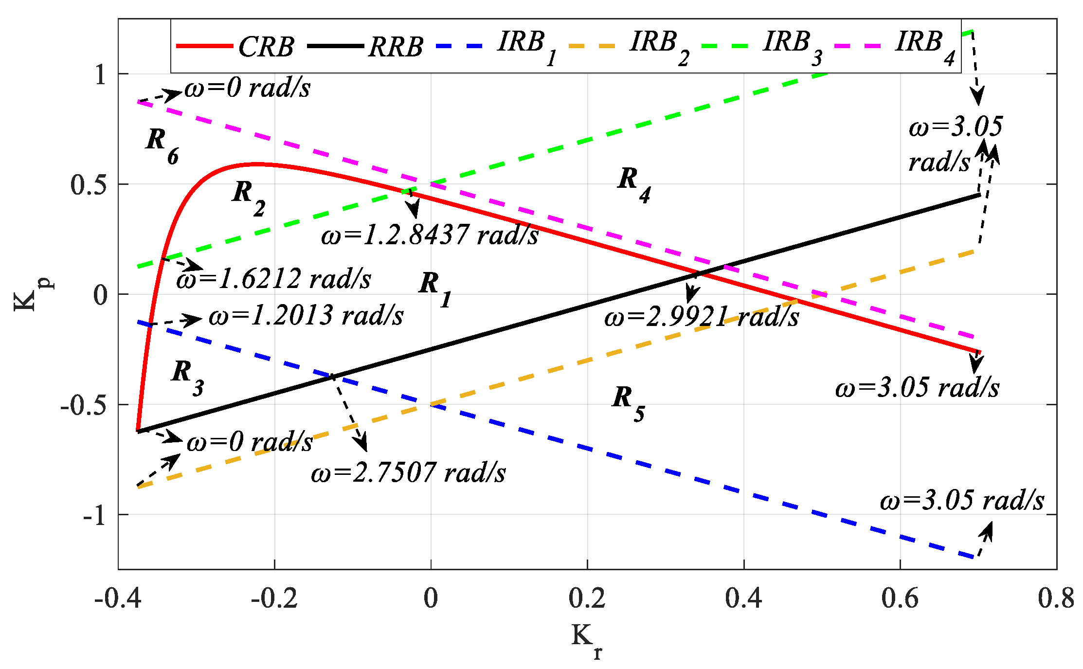
To determine the stable region, the SBL curve for the frequency range ω ∈ [0, 3.05] rad/s was plotted as shown in Figure 24 with the help of RRB, IRB, and CRB equations.

It has been explained in Section 3.2 that, in processes with an equal order of numerators and denominators as in (28) (n = m), IRB lines can affect stability, but not all IRB lines always affect stability. Therefore, when determining the stable controller parameter region in such time-delay processes, all IRB lines calculated by (11) are plotted. Then, regions are determined according to the intersection of RRB, IRB, and CRB lines, and the stability test of these regions is performed. In Figure 24, it is aimed to find the (K_r, K_p) parameter region that stabilizes, via Hurwitz stabilization, the characteristic polynomial in (4) from the SBL obtained for the frequency range ω ∈ [0, 3.05]. For this reason, the (K_r, K_p) parameter test points were selected from the region bounded by the RRB, IRB, and CRB lines and the regions outside this region, and the stability of (4) was analyzed. 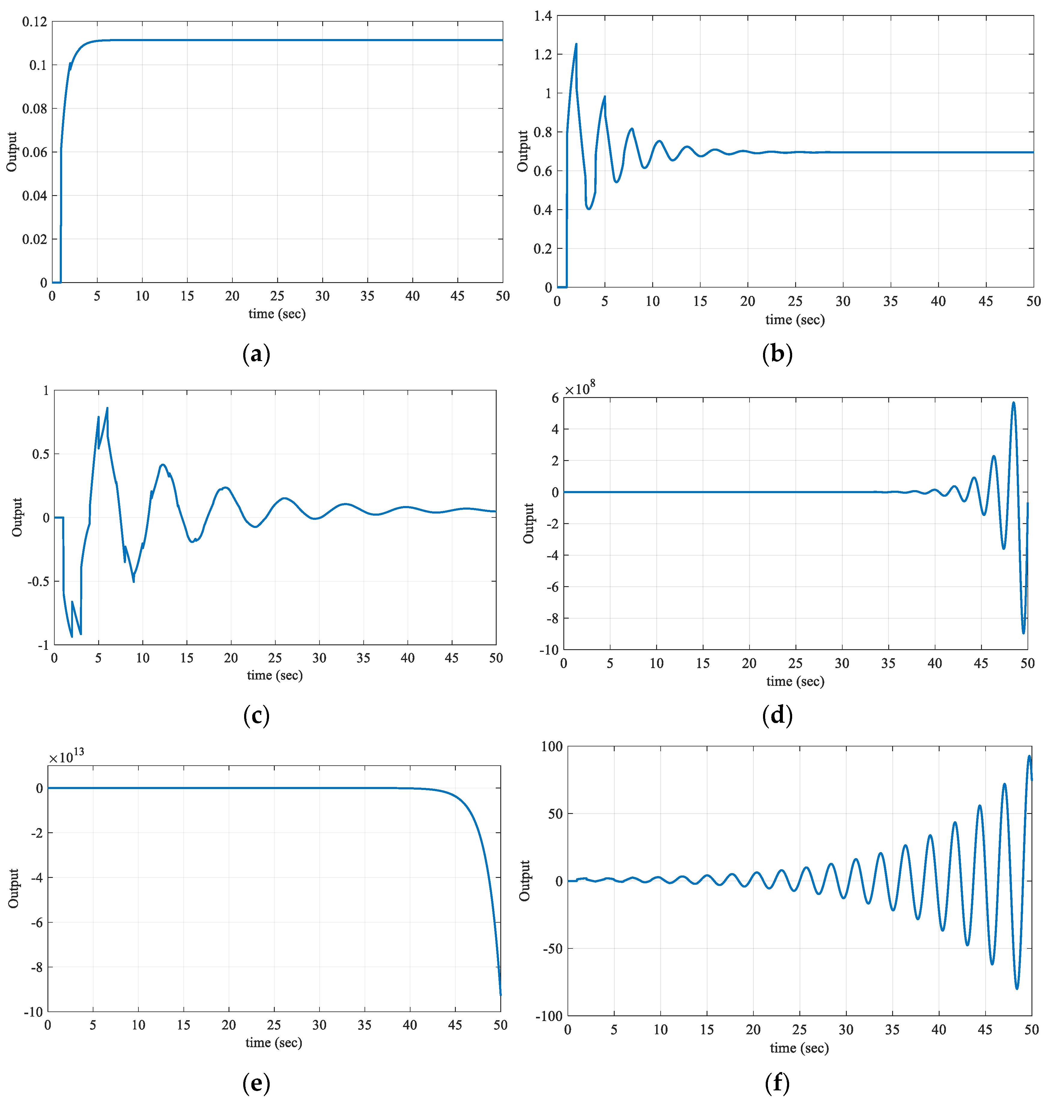Test points (−0.00046, 0.03), (−0.1857, 0.3838), (−0.3018, −0.2868), (0.2346, 0.5074), (0.2926, −0.4368), and (−0.3350, 0.6132) were selected from the determined R₁, R₂, R₃, R₄, R₅ and R₆ regions, respectively. The plotted unit step responses for these test points are presented in Figure 25.

When the unit step responses in Figure 25 obtained for the regions in Figure 24 are analyzed, it is seen that the characteristic equations for the test point in regions R₁, R₂, and R₃ have only the left half-plane pole, thus, they are stable regions. As the characteristic equations written in (4) for the test points selected from the R₄, R₅, and R₆ regions have the right half-plane pole, these regions are unstable regions, as shown in Figure 25. In other words, the PR controller to be designed for a (K_r, K_p) controller parameter pair selected from these regions (R₄, R₅, and R₆) will not provide the stability of the system in (28). Therefore, the stable region is the R₁, R₂, and R₃ regions covering the frequency range ω ∈ [0, 2.9921] rad/s, i.e., the regions bounded by the CRB and RRB lines. Here, the boundary lines obtained by equations IRB₂ and IRB₄ do not intersect the CRB and RRB lines and therefore do not affect the stable region. Although the boundary lines obtained with the IRB₁ and IRB₃ equations intersect with CRB and RRB lines, they do not affect stability.

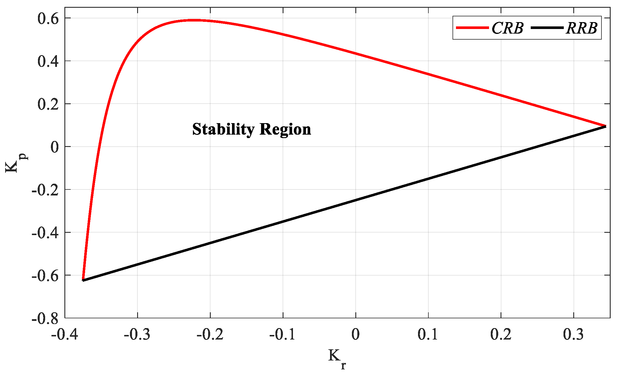
Accordingly, considering the frequencies of the boundary points where the CRB and RRB lines intersect, the stable controller parameter region of the system in (28) for h = 1 is drawn as shown in Figure 26.

As can be seen from Figure 26, the stability region for the PR controller is found as the intersection area of the RRB and CRB lines. Accordingly, the K_p and K_r controller parameter ranges that make the system stable are determined as [−0.625 0.59] and [−0.375 0.344], respectively. Accordingly, SBL graphs for the controller parameter range K_{r_fixed} = [−0.3:0.1:0.3] are drawn as shown in Figure 27, with the RRB defined by the line equation K_i = 0 and the CRB equations calculated by (16) and (17).

Figure 27 was obtained by plotting the K_p-K_i SBLs in the frequency range ω ∈ [0, ω_max] rad/s for K_{r_fixed} = −0.3, −0.2, −0.1, 0, 0.1, 0.2, and 0.3. Accordingly, the ω_max values for these K_{r_fixed} values are 2.1707, 2.6155, 2.7816, 2.868, 2.9212, 2.9570, and 2.9829 rad/s, respectively. The stable K_i controller parameter range will be determined for an SBL selected from the SBL graphs of the system with a PIR controller designed for different K_{r_fixed} values in Figure 27. Therefore, according to the SBL graph of the PIR controller designed for K_{r_fixed} = −0.1, the K_i controller parameter range that makes the system stable is [0 0.408]. SBL graphs for K_{i_fixed} values to be selected from the K_i controller parameter range are obtained with the help of the RRB line defined by $K_p-K_r=-0.25$, a CRB line to be drawn with the help of (19) and (20), and IRB lines to be obtained with the help of (11), if any. Accordingly, SBL plots for the controller parameter range K_{i_fixed} = [0:0.1:0.4] are drawn as shown in Figure 28.

Figure 28 was obtained by plotting K_r-K_p SBLs in the frequency range ω ∈ [ω_min, ω_max] rad/s for K_{i_fixed} = 0, 0.1, 0.2, 0.3, and 0.4. For these K_{i_fixed} values, the frequency ranges that make the system stable are ω ∈ [0, 2.9921], [0.378, 0.947], [0.54, 2.9], [0.672, 2.853], and [0.79, 2.803] rad/s, respectively. It is seen that the stable K_r-K_p controller parameter region becomes smaller as the K_{i_fixed} value increases.

It is seen from Figure 28 that the RRB line defined by the equation of $K_p-K_r=-0.25$ is the determinant of the stability boundary only in the case of K_{i_fixed} = 0. Moreover, in the stability analysis in Figure 24 for K_i ≠ 0, it was shown that the IRB₂ and IRB₄ boundary lines do not intersect the CRB and RRB lines and do not affect the stable region. The IRB₁ and IRB₃ boundary lines intersect the CRB and RRB lines, but do not affect stability. The positions of these IRB₁, IRB₂, IRB₃, and IRB₄ boundary lines at K_i ≠ 0 are shown in Figure 28a. According to the stability analyses performed here, it is seen that these lines do not separate the system in (28) into unstable regions, and that the stability regions of the system with a PIR controller designed according to different K_{i_fixed} values are shown in Figure 28b.

From the SBL graph for the PR controller in Figure 26, the K_p controller parameter range that makes the system stable was determined as [−0.625 0.59]. Accordingly, for a K_{p_fixed} selected from the K_p controller parameter space, SBL is generated by an RRB line defined by the equation K_i = 0 and a CRB line to be drawn with the help of (16) and (17). Accordingly, SBL graphs for the controller parameter range K_{p_fixed} = [−0.6:0.2:0.4] are drawn as shown in Figure 29.

Figure 29 was obtained by plotting K_r-K_i SBLs in the frequency range ω ∈ [ω_min, ω_max] rad/s for K_{p_fixed} = −0.6, −0.4, −0.2, 0, 0.2, and 0.4. In the stability analyses for these K_{p_fixed} values, the frequency ranges ω ∈ [0, 0.2555], [0, 0.7869], [0, 1.1146], [0, 1.4009], [1.6831, 2.9681] and [1.9666, 2.89] rad/s were found, respectively. It is seen that the stable K_r-K_i controller parameter region increases as the value of K_{p_fixed} increases.

The above analyses were performed for h = 1, and the analyses were repeated to interpret the effect of different values of h on SBL. In this regard, the cases of h > $\theta$, h = $\theta$, and h < $\theta$ are examined. Although the case of h = $\theta$ is h = 1 as examined above, the analyses for the cases of h = 0.5 (h < $\theta$), and h = 1.1 (h > $\theta$) are repeated as follows.

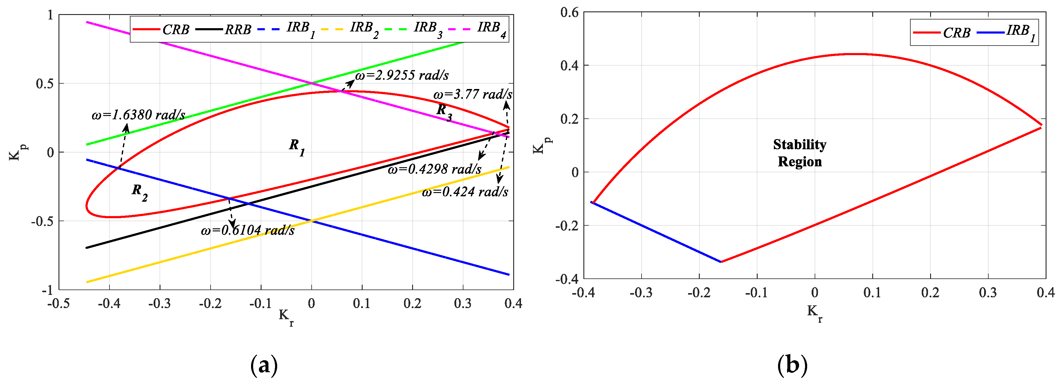
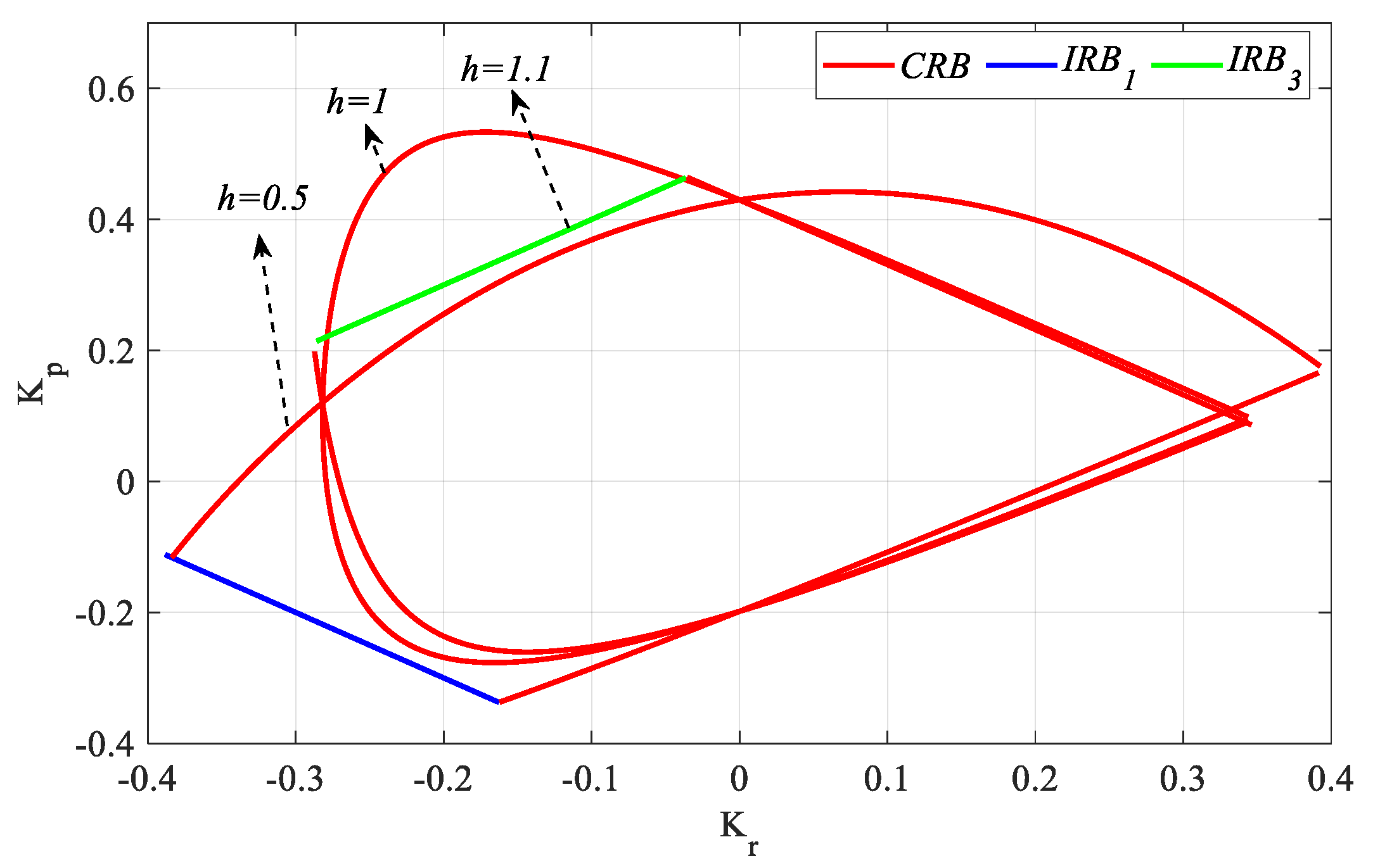
In Figure 30a, the SBL graph for the PR controller is drawn for h = 0.5 in the frequency range ω ∈ [0, 5] rad/s. As can be seen from Figure 30a, lines CRB, RRB, IRB₁, and IRB₄ intersect each other, while lines IRB₂ and IRB₃ are tangent to CRB and RRB. Stability analysis was performed for the three closed regions (R₁, R₂ and R₃) resulting from the intersection of the CRB, RRB, IRB₁, and IRB₄ lines. It was observed that the PR controllers designed for K_r-K_p selected from the closed R₂ and R₃ regions make the process in (28) stable, while the controller parameter pair selected from the R₁ region makes the system unstable. As a result of this analysis for h < $\theta$, it was seen that the CRB, RRB, and IRB₁ lines affect stability, while the IRB₄ line does not. The IRB₂ and IRB₃ lines did not play a role in determining the stability as they passed tangentially to CRB and RRB. Accordingly, the stability region for h = 0.5 is drawn in Figure 30b by considering the frequencies of the boundary points where the CRB, RRB and IRB₁ lines intersect.

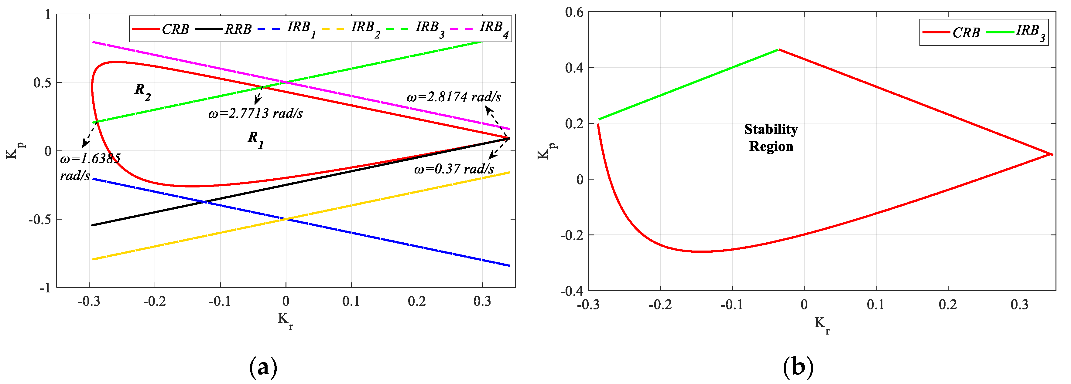
Figure 31a shows the SBL curve for h = 1.1 in the frequency range ω ∈ [0, 3] rad/s. As can be seen from Figure 31a, the lines CRB, RRB, IRB₁, and IRB₃ intersect each other, and the lines IRB₂ and IRB₄ are tangential to CRB and RRB. Stability analysis was performed for the three closed regions (R₁, R₂ and R₃) resulting from the intersection of the CRB, RRB, IRB₁ and IRB₃ lines and it was observed that the PR controllers designed for the controller parameter pair (K_r, K_p) selected only in the R₁ region make the process in (28) stable, while the controller parameter pair selected in the R₂ and R₃ regions make it unstable. As a result of this analysis for h > $\theta$, it is seen that CRB, RRB, IRB₁, and IRB₃ lines affect stability. IRB₂ and IRB₄ lines did not play a role in determining stability as they passed tangentially to CRB and RRB. Accordingly, the stable region was found to be the closed R₁ region, and the stability region for h = 1.1 was drawn in Figure 31b by considering the frequencies of the boundary points where the CRB, RRB, IRB₁, and IRB₃ lines intersect.

From Figure 30b and for h = 0.5, the K_p and K_r controller parameter ranges that stabilize the system are [−0.37 0.44] and [−0.42 0.38], respectively. Similarly, from Figure 31b, the K_p and K_r controller parameter range that makes the process stable for h = 1.1 is determined as [−0.4 0.41] and [−0.35 0.34], respectively. For the K_{r_fixed} = −0.1 and 0.1 values selected from the common stable controller parameter range, RRB is defined by K_i = 0 and CRB equations are calculated with the help of (16) and (17). K_p-K_i SBL plots are obtained as shown in Figure 32.

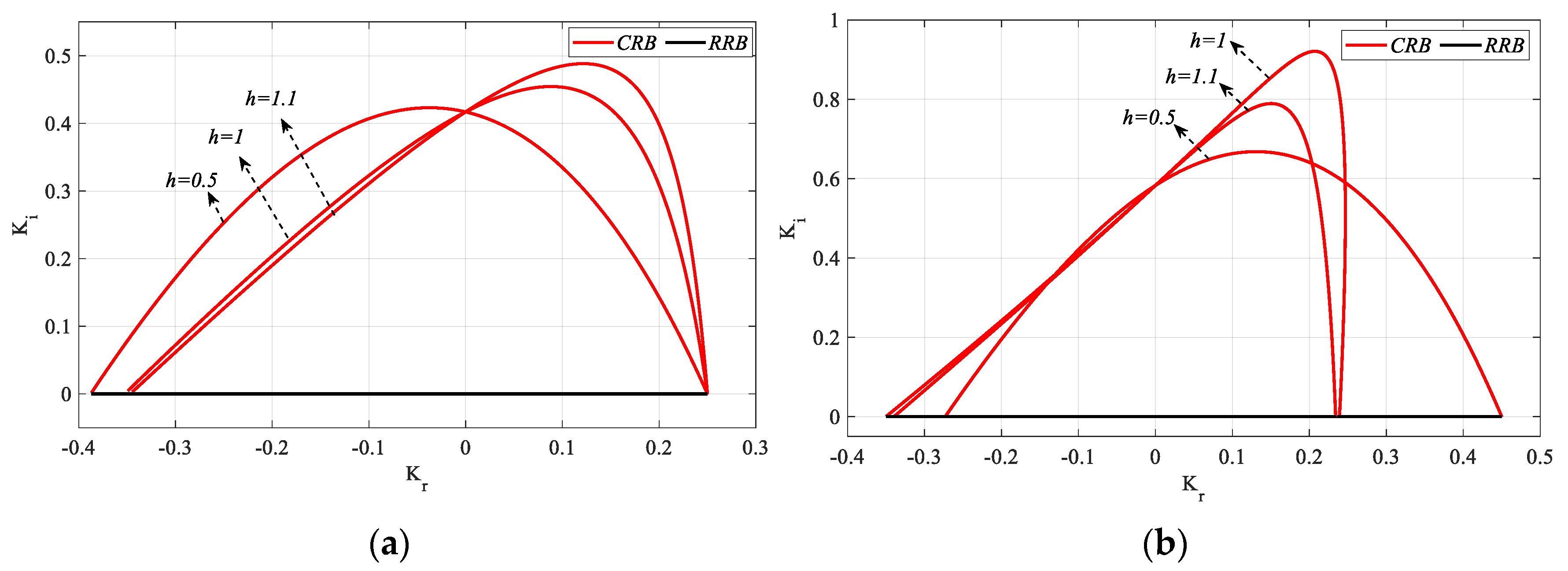
In Figure 32a, the ω_max values for K_{r_fixed} = −0.1 and h = 0.5, 1, and 1.1 are 2.6255, 2.7816, and 2.8717 rad/s respectively, and in Figure 32b, the ω_max values for K_{r_fixed} = 0.1 and h = 0.5, 1 and 1.1 are 3.1093, 2.9212, and 2.8646 rad/s respectively. As the controller will turn into a PI controller for K_r = 0, the value of h will have no effect on SBL, and it will be the same as K_{r_fixed} = 0 in Figure 27. The K_r-K_p SBL curves and stability regions for K_{i_fixed} = 0.1 and h = 0.5 and 1.1, which are selected from the common stable controller parameter ranges of the SBL curves in Figure 32, are presented in Figure 33 and Figure 34.

In Figure 33a, the CRB curve for K_{i_fixed} = 0.1 and h = 0.5 is plotted in the frequency range ω ∈ [0.424, 3.77] rad/s. In the analysis for K_{i_fixed} = 0 in Figure 30a, it was found that the boundary lines determining the stability were the CRB, RRB, and IRB₁ lines. When the same analysis was performed for K_{i_fixed} = 0.1, it was found that CRB and IRB₁ lines affect stability, while RRB does not affect stability as a result of it not intersecting with CRB. Accordingly, considering the frequency points where the CRB and IRB₁ lines intersect, the stable controller region for K_{i_fixed} = 0.1 and h = 0.5 is obtained as shown in Figure 33b. Similarly, the CRB curve for K_{i_fixed} = 0.1 and h = 1.1 in the frequency range ω ∈ [0.37, 2.8174] rad/s is obtained as shown in Figure 34a. In the analysis for K_{i_fixed} = 0 in Figure 31a, it was found that the boundary lines determining the stability were CRB, RRB, IRB₁, and IRB₃ lines. When the analysis was repeated for K_{i_fixed} = 0.1, it was found that only CRB and IRB₃ lines affected stability, and that IRB₁ and RRB did not affect stability because of they do not intersect with CRB. Accordingly, considering the frequency points where the CRB and IRB₃ lines intersect, the stable controller region for K_{i_fixed} = 0.1 and h = 1.1 is obtained as shown in Figure 34b.

With the values obtained from Figure 28b, Figure 33b and Figure 34b, the SBL for the stable controller parameter regions for K_{i_fixed} = 0.1 and h = 0.5, 1, and 1.1 are drawn as in Figure 35.

When Figure 35 is examined, the stable K_r-K_p parameter region narrows as the h value increases in the case of K_{i_fixed} = 0.1. From Figure 26, Figure 30 and Figure 31, the stable K_p controller parameter ranges were found to be [−0.37 0.44], [−0.625 0.59], and [−0.4 0.41] for h = 0.5, 1, and 1.1, respectively. Accordingly, K_r-K_i SBL graphs for K_{p_fixed} 0 and 0.2 selected from these stable regions were obtained and are shown in Figure 36.

As illustrated in Figure 36a, the frequency ranges that ensure system stability for h = 0.5, 1, and 1.1 are presented as ω ∈ [0, 1.8759], [0, 1.4009], and [0, 1.3341] rad/s, respectively. Similarly, Figure 36b demonstrates the corresponding frequency ranges for h = 0.5, 1, and 1.1, namely ω ∈ [1.6831, 2.9681] and [1.6029, 2.8635] rad/s. When Figure 36a is examined, as the h value increases when K_{p_fixed} = 0, the stable K_r parameter range decreases relatively, while the stable K_i parameter range increases. Similarly, in the analysis made for K_{p_fixed} = 0.2 in Figure 36b, it is seen that, as the h value increases, the stable K_r range decreases significantly, while the stable K_i range increases. The unit step responses of the SBL curves obtained for h = 0.5, 1, and 1.1 in Figure 32a, Figure 35 and Figure 36b were analyzed for K_p, K_i, and K_r values selected from the common stability regions. 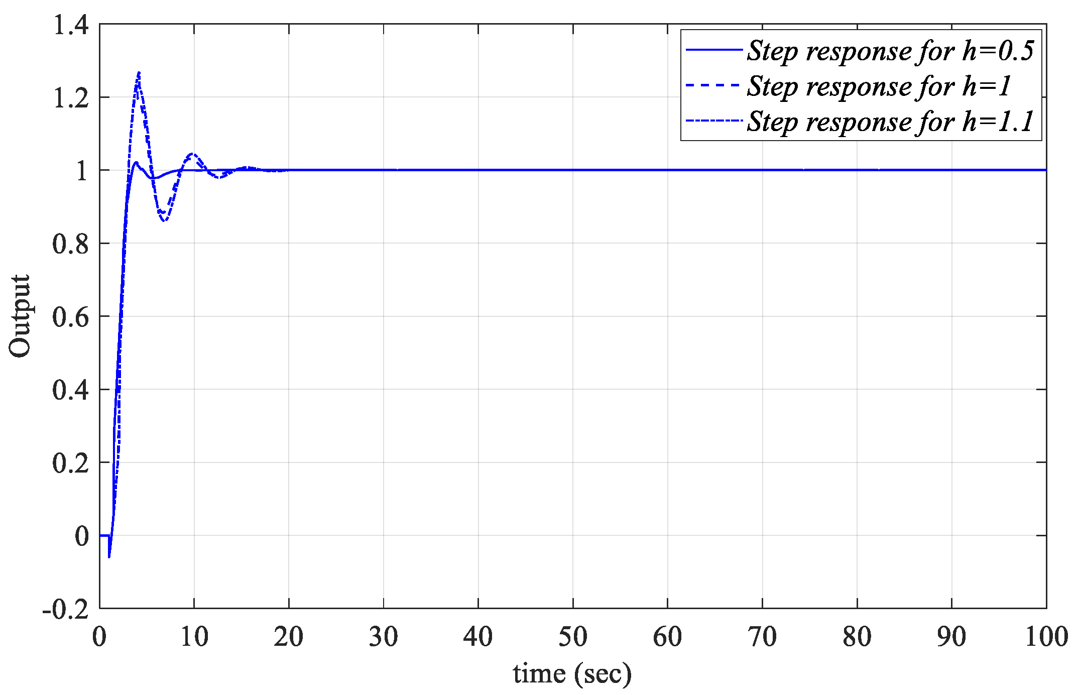It can thus be expected of the PIR controllers designed for the parameters selected from these regions that they will ensure the stabilizing of the G_p3 process in Figure 1 in the instances h = 0.5, 1, and 1.1. 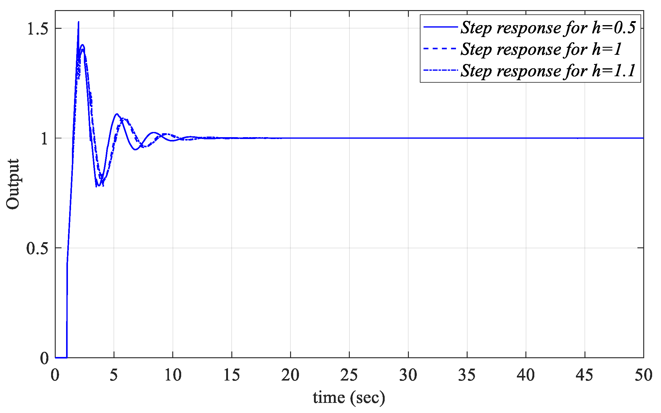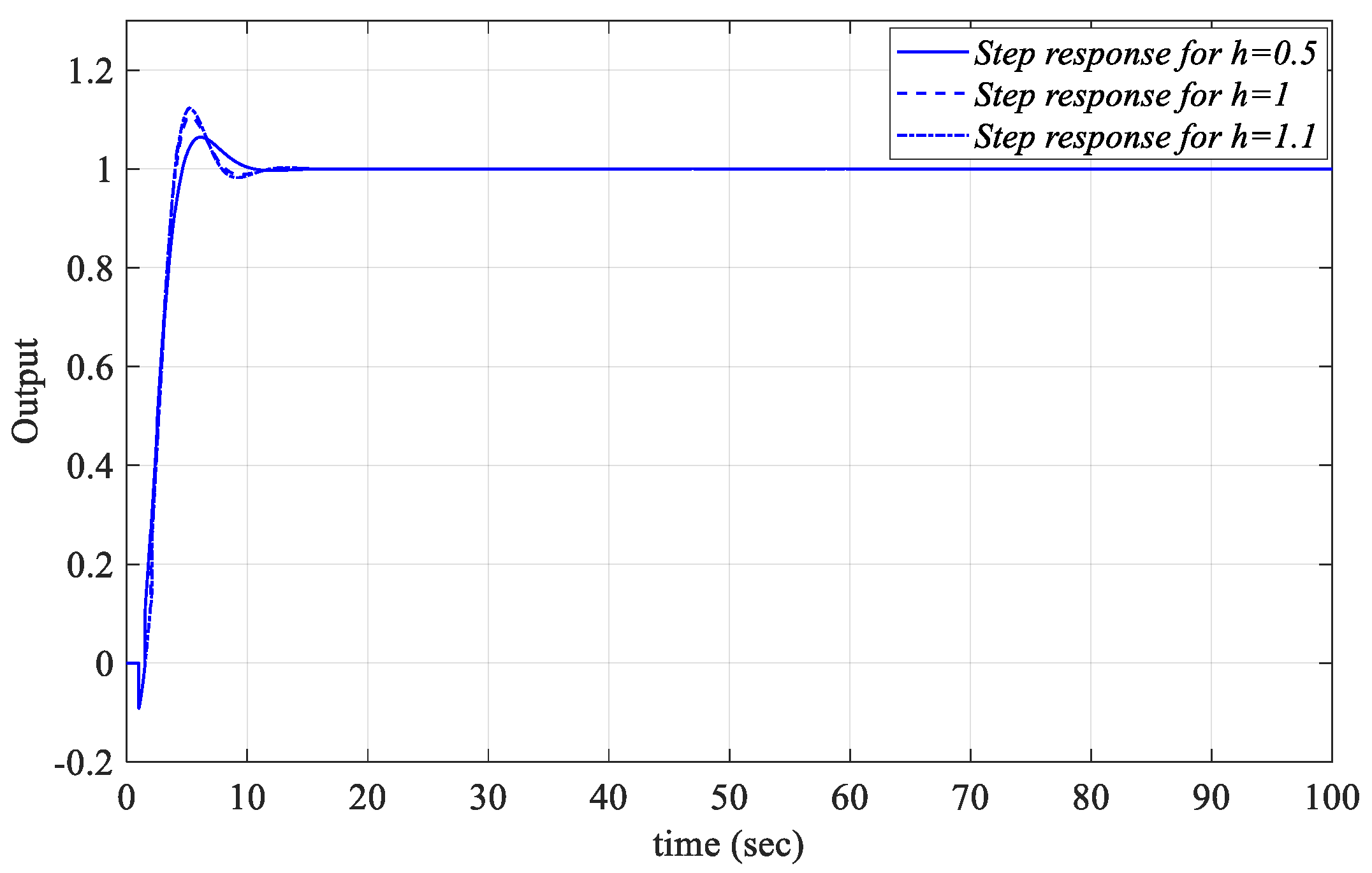In this context, the unit step responses of the control system given in Figure 1 obtained by applying the PIR controllers designed for K_p =−0.0297 and K_i =0.1183 values selected from the common region of the K_p-K_i SBL curves drawn by taking h=0.5, 1 and 1.1 values in Figure 32.a when K_{r_fixed} =−0.1 are shown in Figure 37. The PIR controllers are designed for the controller parameter values K_p = −0.0544 and K_r = −0.0460, which are selected from the K_r-K_p SBL graph in Figure 35, drawn for K_{i_fixed} = 0.1. The unit step responses for different h values are shown in Figure 38. Similarly, the controller parameter values K_i = 0.2833 and K_r = −0.0460 are selected from the K_r-K_i SBL curve in Figure 36b, obtained for K_{p_fixed} = 0.2, and the unit step responses for h = 0.5, 1, and 1.1 are presented as in Figure 39.

When Figure 37, Figure 38 and Figure 39 are examined, it is seen that the PIR controllers designed for the parameters selected from the common stability regions of the SBL curves drawn for the cases h = 0.5, 1 and 1.1 control the G_p3 time-delay process with a first-order transfer function in the numerator and denominator in Figure 1 in a stable manner.

6. Conclusions

The main objective of this study was to analytically determine the complete set of stabilization parameters for PIR controllers in time-delay systems. For this purpose, in this study, the stability region of the controller parameters is obtained by extracting the SBL equations of the PIR controller. This is the first time this has been achieved in the literature. With the proposed method, analytical and graphical solutions are presented to obtain stable regions in the two-dimensional controller parameter space. As the PIR controller has four tunable parameters (K_p, K_i, K_r, and h), in order to design in the two-dimensional controller parameter space, firstly, the controller time delay (h) is taken as a constant value. Then, for a fixed value of K_p in the (K_i, K_r) plane, for a fixed value of K_i in the (K_r, K_p) plane and for a fixed value of K_r in the (K_p, K_i) plane, the calculations of the region of the PIR controller parameters that make the time-delay closed-loop control system stable are given. For these three cases (constant K_p, constant K_i, and constant K_r), the RRB, IRB, and CRB boundary line equations for obtaining the SBL were obtained. With the help of these lines, the SBL was drawn, and, in order to find the stable parameter region, test points were selected from the regions within the SBL, and stability analyses were performed on the unit step responses of these points. The analyses were repeated for both stable and unstable time-delay processes, and the stable controller region of the system with PIR controller was found. Furthermore, it is explained with mathematical equations that IRB lines will only appear in time-delay processes with equal orders of the numerator and denominator polynomial, and this is proved on a time-delay process with equal orders of the first-order numerator and denominator polynomial. The analyses are repeated for three different cases where the controller time delay is greater than, equal to, and less than the process time delay, and the effect of the controller time delay on the stable controller region is observed. Accordingly, it is observed that, as the value of the controller time delay increases, the stable controller parameter space that makes the closed-loop system generally narrows. As a result of all analyses, the stability regions of time-delay systems with PIR controllers are found and presented to the literature. In future studies, robustness analyses will be performed to evaluate the robustness of the PIR controller against measurement noise and disturbances.