Design Optimization of an Inclined Inlet Channel, an Archimedean Spiral Basin, and a Discharge Cone in a Gravitational Vortex Turbine

Abstract

This research focused on optimizing the design of a gravitational vortex turbine by refining the inclined inlet channel, the Archimedean spiral basin, and the discharge cone to improve system efficiency. The study employed computational fluid dynamics (CFD) simulations combined with response surface methodology (RSM) to systematically analyze the impact of key geometric parameters on energy extraction. The investigated parameters included the inclined angle of the channel, outlet diameter ratio, inlet channel height ratio, and inlet channel width ratio. Among these, the outlet diameter ratio was found to have the most significant influence on efficiency. The numerical results were validated through experimental testing, confirming the accuracy of the optimized design, which achieved a maximum efficiency of 87.7% at 71.54 RPM. This enhancement highlights the novelty of incorporating an Archimedean spiral basin and an inclined inlet channel, demonstrating the effectiveness of the proposed optimization methodology in maximizing energy extraction.

1. Introduction

The demand for energy to support social and economic development, as well as to enhance human well-being and health, is expanding quickly due to population and economic growth, especially in developing economies [1,2].

According to estimates by international organizations, demographic projections suggest that the global population will reach 9.7 billion by 2050 [3], with developing countries experiencing the greatest expansion [4,5]. This demographic surge, coupled with urbanization and economic development, will intensify the need for energy to meet basic requirements such as housing, transportation, industrial production, and services [6]. The challenge lies in guaranteeing universal access to sustainable energy sources for all while minimizing additional pressure on natural resources and the environment. Emerging economies, such as India, China, and nations across the African continent, will be at the forefront of this accelerated growth in both population and energy demand [7,8]. India is projected to become the world’s most populous country by the mid-century [9], while Africa will experience a substantial increase in its young population and urbanization rates [10,11]. This scenario underscores the urgent need to invest in clean technologies and sustainable energy infrastructure to ensure reliable and efficient energy supply.

The current energy mix reveals that approximately 80% of global energy consumption comes from non-renewable sources, such as natural gas, coal, and oil, which have historically been the backbone of worldwide energy production [12,13]. On the other hand, renewable energy has been gaining prominence in recent decades, accounting for about 20% of global energy consumption [14,15]. Hydropower leads this segment with roughly 10%, followed by wind, solar, and biomass energy, which together make up the remainder [16,17]. Hydropower plays a pivotal role in the global energy landscape due to its reliability and sustainability. Among the innovative advancements in this field, gravitational vortex turbine (GVT) technology has emerged as a groundbreaking solution [18,19]. Unlike traditional hydropower systems, which often require large-scale infrastructure and significant environmental alterations, GVTs harness the natural rotational energy of water in a vortex formation [20,21].

Research on gravitational vortex generation systems is still evolving, placing the technology in an early stage of development [18,22]. To enhance efficiency, Velasquez et al. [19] applied surface methodology (RSM) to optimize key geometric parameters affecting circulation. The highest circulation of 2.089 m²/s was achieved were $d/D=$ 0.167, $H/D=$ 1.840, $w/D=$ 0.2, $h/D=$ 0.599, $L/D=$ 0.500, and $\gamma =$ 179.976°. Edirisinghe et al. [23] optimized a vortex turbine in a conical basin using CFD analysis, modifying the blade inclination, height, vertical twist, and horizontal curvature. Performance was evaluated through water–air interface, pressure, and velocity analyses. Aligning the blade inclination with the basin and increasing the blade height improved the efficiency by expanding the vortex-affected area. The horizontal curvature reduced back pressure and enhanced pressure differences, achieving the highest efficiency of 40.4%. Jianget al. [24] conducted a two-phase numerical investigation using ANSYS Fluent. The first phase identified the optimal vortex location in a conical basin by analyzing notch angles, conical angles, basin shapes, and diameters. The second phase focused on optimizing turbine blade geometry for maximum power output and structural durability through hydro—structural interaction (HSI) analysis. Four hydro-rotor models—thin/slim, aerofoil-based, Savonius, and high-twist blades—were evaluated. The results indicated that a circular basin (1000 mm diameter) with a 13° notch angle and 14° conical angle enhanced vortex performance. Among the rotors, Model III demonstrated the highest torque and power output, making it the best candidate for hydropower applications. Betancour et al. [25] improved GVT design through numerical simulations and optimization. They analyzed four rotor configurations using the 6-DoF method in ANSYS Fluent to identify the most efficient geometry. The selected rotor was optimized via RSM, considering key factors like blade number, twist angle, and geometric ratios. The optimized turbine achieved a maximum efficiency of 52.2%. Mobeen et al. [26] analyzed the impact of key parameters (flow rate, cone angle, blade position, and blade type) on torque generation and efficiency. Using Design of Experiments (DOE) and Taguchi analysis, optimal conditions were identified through experimental testing. A turbine was fabricated and optimized using Minitab software, which predicted a maximum torque of 5.788 Nm at a flow rate of 0.016 L/s. Velasquez et al. [20] applied RSM to optimize the runner design of a GVT. The effects of runner position, blade number, and the blade-to-basin diameter ratio on turbine efficiency were analyzed. A second-order regression model predicted a maximum efficiency of 65.18%. Across these studies, various optimization methods were employed to enhance the efficiency of gravitational vortex turbines (GVTs). The response surface methodology (RSM) has been widely used to optimize geometric parameters influencing circulation and turbine efficiency [19,20,25]. Computational fluid dynamics (CFD) analysis has also played a key role, particularly in optimizing blade geometry and flow behavior within conical basins [23,24]. Additionally, experimental approaches combined with DOE and Taguchi analysis have been used to identify optimal operational parameters such as flow rate, cone angle, blade position, and blade type [26]. These findings highlight the importance of both numerical and experimental optimization techniques in advancing GVT technology for sustainable energy applications.

This current research focused on optimizing the GVT with the primary objective of maximizing vortex circulation ($\Gamma$). Circulation in a vortex refers to the rotational strength of the water flow, representing the amount of rotational motion per unit of water flow rate. In the context of a GVT, it measures how effectively the water forms and maintains the vortex structure. This optimization was accomplished through the use of RSM. The input variables considered in this study included key geometric characteristics of the turbine’s inlet channel and discharge chamber, such as their dimensions, shapes, and angles. By systematically varying these parameters and analyzing their impact on vortex formation and strength, the study aimed to identify the optimal configuration that enhanced energy extraction efficiency. This approach not only improves the turbine’s efficiency but also provides valuable insights into the design principles that govern gravitational vortex systems, paving the way for more effective and scalable renewable energy solutions.

The optimal geometric configuration of the inlet channel, circulation chamber, and discharge zone was fabricated at a laboratory scale. Its performance in energy conversion was evaluated by measuring the power generated by a rotor placed within the circulation and discharge chamber. For this purpose, an experimental facility specifically designed for the characterization of this type of turbine was utilized. This setup allowed for the assessment and optimization of the turbine’s efficiency, providing valuable insights into its operational behavior and energy transformation capabilities. The novelty of this study lies in the integration of an Archimedean spiral basin and an inclined inlet channel, which were systematically optimized using RSM to enhance energy extraction. These design improvements led to a significant increase in efficiency, demonstrating the potential of this approach. Enhancing the performance of such emerging energy systems is crucial for promoting sustainable and decentralized power generation, particularly in regions with limited access to conventional energy infrastructure.

2. Materials and Methods

2.1. Principles of Turbine Operation

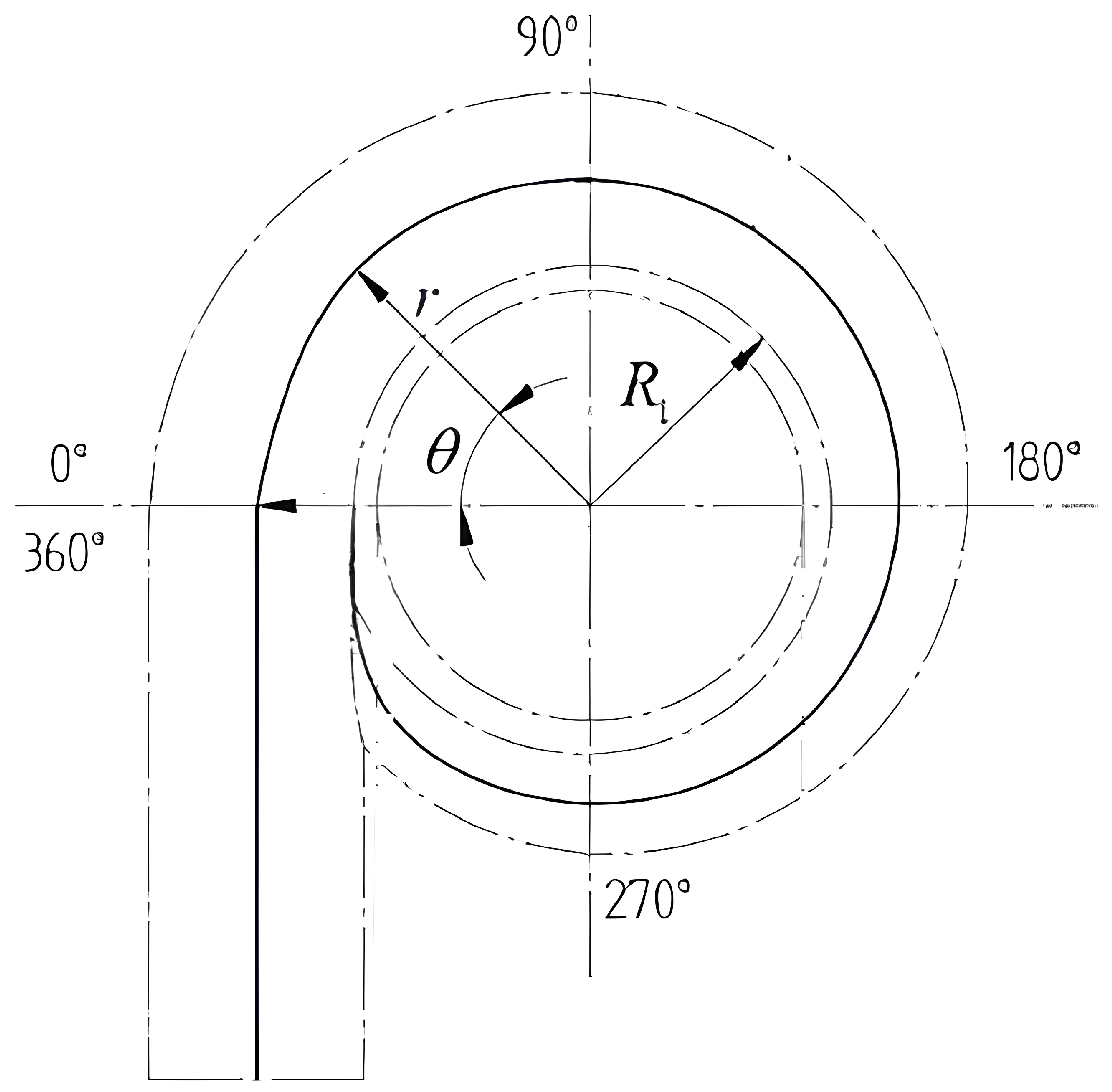
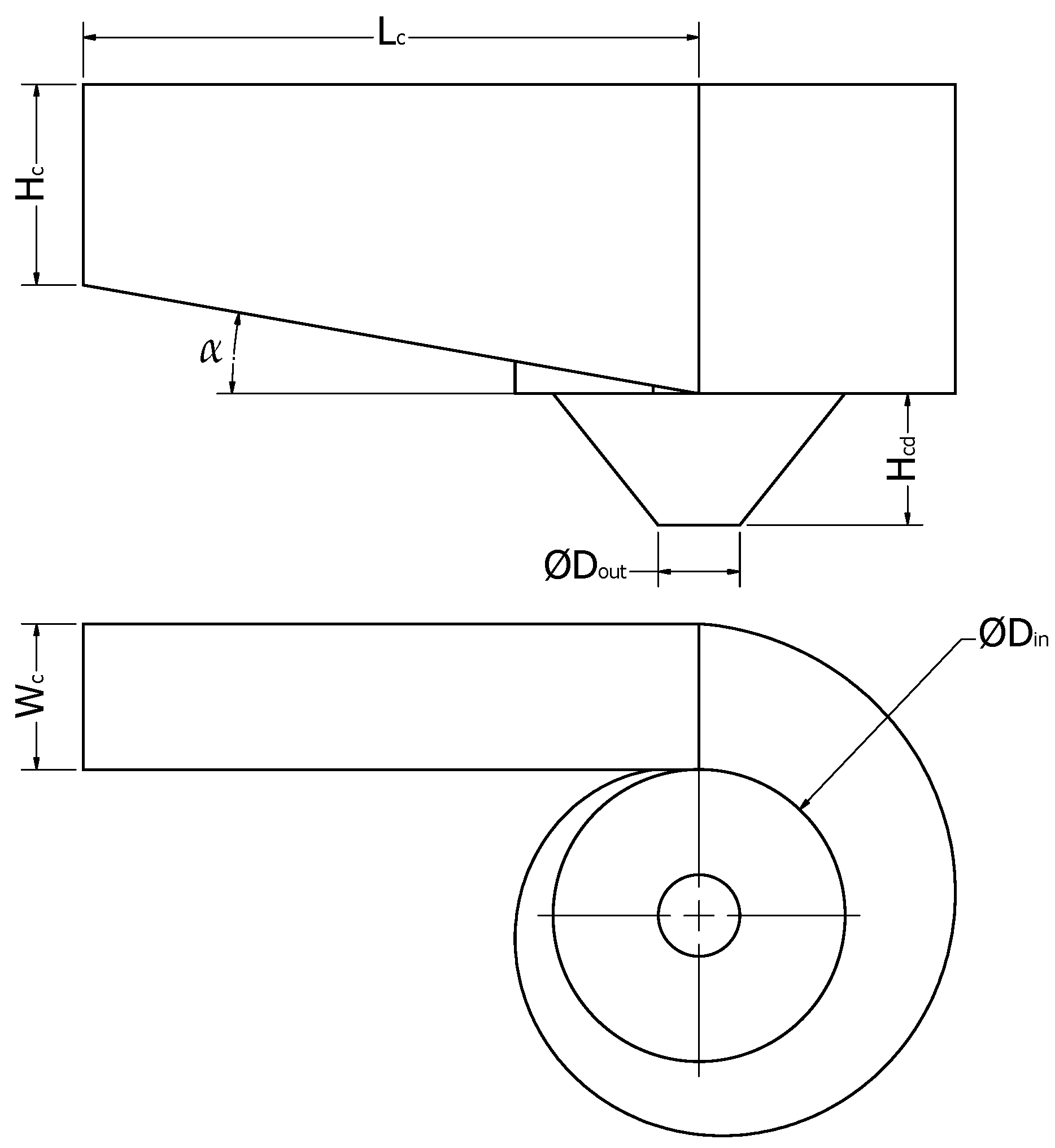
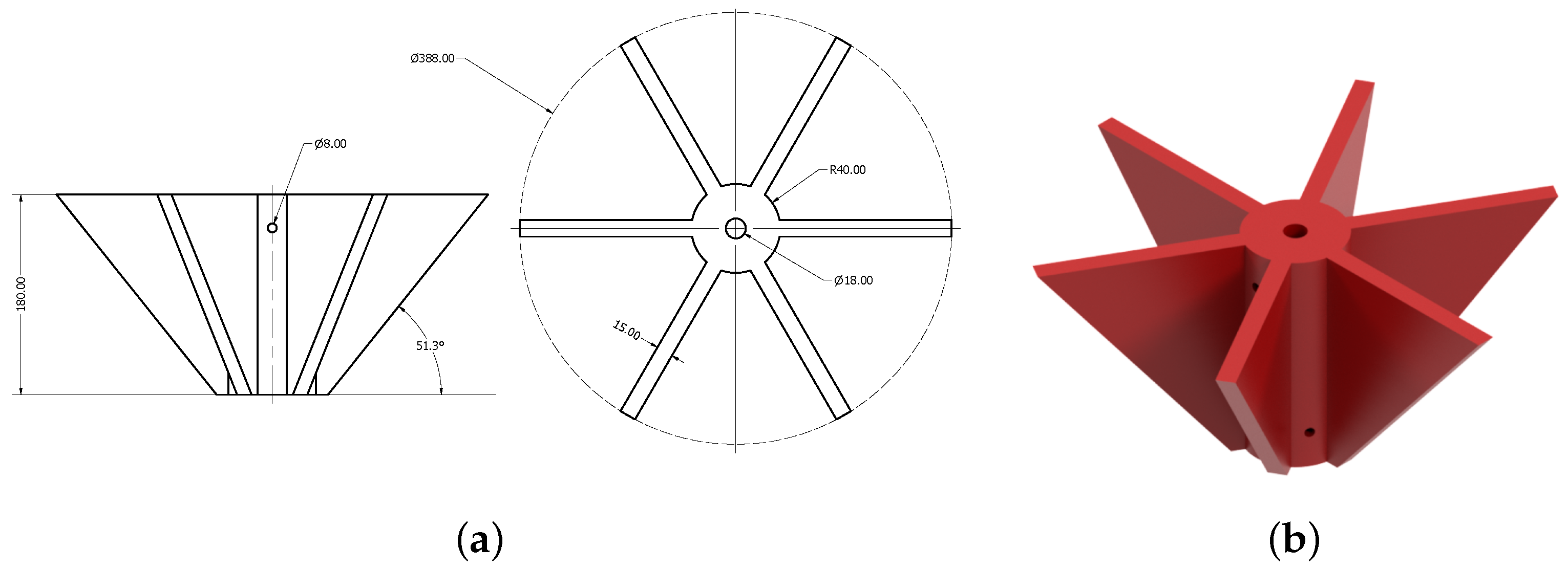
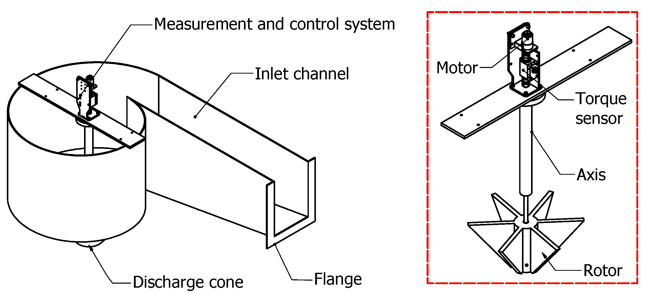
GVT is a system designed to harness energy from water courses in a simple and efficient manner. Unlike conventional hydropower plants that rely on large dams, this technology utilizes the natural flow of rivers or streams to generate electricity with minimal structural intervention [20,21]. Its operation begins with an inlet channel that captures water from a watershed and directs it into a circulation channel. In this channel, the water starts to rotate, forming a vortex due to the interaction between kinetic energy (from the water’s movement) and potential energy (caused by gravity) [27]. The energy from the generated vortex is used to drive a turbine, causing its shaft to rotate. This rotational motion enables a generator to convert mechanical energy into electricity [20]. One of the key benefits of this system is that it eliminates the need for water storage in a reservoir, allowing it to operate without significantly altering the natural course of rivers. This characteristic makes it a less invasive alternative to traditional hydropower plants, minimizing disturbances to aquatic ecosystems and surrounding communities. The available power in GVT can be calculated using the equation for hydropower, which is given by $P=\rho gQH$, where P represents the available power, g is the acceleration due to gravity, $\rho$ is the density of water, Q is the flow rate, and H is the head, which is the height difference between the water source and the turbine. The power output of the rotor is determined by the equation $P_{out}=T\omega$, where T is the torque and $\omega$ is the angular velocity of the rotor. Finally, the efficiency ($\eta$) is calculated as the ratio of the power output to the available power, given by Equation (1) [20,23]:

$$\eta ={\displaystyle \frac{P_{out}}{P}}={\displaystyle \frac{T\omega }{\rho gQH}}$$

(1)

2.2. Turbine Design

The design of the inlet channel and discharge cone is crucial for the successful development of a GVT, as these components govern the flow dynamics and ensure efficient energy extraction by the turbine [23,28]. For the design of the gravitational vortex system, an enveloping inclined inlet channel was selected, with its geometry was defined by the Archimedean spiral. The Archimedean spiral was chosen due to its innovative nature and the lack of prior references in the literature. This design allows the fluid to flow smoothly along the entire envelope, facilitating a gradual descent into the discharge cone. The mathematical equation representing the Archimedean spiral in polar coordinates is Equation (2) [29]:

$$r=a+b\theta$$

(2)

where r is the radius of the spiral as a function of the angle $\theta$, a is a parameter that defines the initial radial offset (in many cases, $a=0$ if the spiral starts at the origin), b is a constant that controls the spacing between the arms of the spiral, and $\theta$ is the angle in radians. Figure 1 shows a general diagram of the Archimedean spiral, illustrating its structure and main features.

For the discharge, the conical geometry was selected due to its ability to maximize water velocity. The increase in velocity generates higher vorticity, resulting from the rapid movement of air induced by the water flow in this region, which, in turn, enhances efficiency when utilized with a turbine.

In the design of the cone, two key parameters were considered: the total height of the cone and the outlet diameter. These parameters, along with the height, width, and inclination of the channel, were optimized through RSM. This approach helped establish a variation range and identify the optimal values for these geometric parameters, ensuring that the discharge cone and inlet channel design maximized circulation and overall system performance. Figure 2 illustrates the selected geometric parameters for the study, where $\alpha$ is the inclined angle of the channel, $D_{out}$ is the outlet hole diameter, $W_c$ is the inlet channel width, $H_c$ is the inlet channel height, and $D_{in}$ is the inlet diameter.

2.3. Application of RSM in Design Optimization

RSM is an optimization strategy that employs mathematical and statistical tools to analyze cases where a target variable depends on other independent variables [30,31]. This methodology allows for the visualization of the target variable through a plane or contour plot. To apply RSM for optimizing a variable, the process begins with defining an appropriate experimental design (DOE) that captures the influence of key geometric variables on the objective variable (Y). This step ensures that the selected independent variables ($X_i$) provide sufficient information about the system’s behavior [30]. Once the DOE is established, a statistical model is fitted to describe the relationship between the independent variables and the objective variable, serving as the foundation for further analysis. The next step involves optimizing the independent variables by determining the factor levels that either maximize or minimize the objective variable, depending on the study’s goals. Through this structured approach, RSM enables a systematic exploration of the design space, allowing researchers to refine performance and achieve precise, data-driven optimizations.

In this study, an exhaustive selection of independent variables was conducted to ensure a clear and meaningful relationship with the response variable, which, in this case, is the water circulation in the cone region. Among the most common experimental designs used in RSM are Box–Behnken designs and central composite designs (CCDs) [32,33,34]. These designs offer significant advantages, as they allow for an efficient mapping of the response surface with fewer experimental points compared to full factorial designs while maintaining a high accuracy in exploring the experimental space [35].

In this study, CCD was selected to support the response surface analysis, using the independent variables described in

Table 1. Independent factors and their levels for the experimental design.

Factor	Variable	−1	0	+1
$\alpha$	Inclined angle of the channel [°]	6	8	10
$D_{out}/D_{in}$	Outlet diameter ratio	0.130	0.205	0.280
$H_c/D_{in}$	Inlet channel height ratio	1.06	1.24	1.42
$W_c/D_{in}$	Inlet channel width ratio	0.32	0.41	0.50

as factors. The selected independent variables were the inclined angle of the channel ($\alpha$), the outlet diameter ratio ($D_{out}/D_{in}$), the inlet channel height ratio ($H_c/D_{in}$), and the inlet channel width ratio ($W_c/D_{in}$). Each of these factors plays a crucial role in the system’s performance: the inclined angle of the channel affects the flow dynamics by increasing its velocity before reaching the chamber due to the additional height; the inlet channel height and the inlet channel width influence the incoming flow rate, which, in turn, alters the flow velocity; and the outlet diameter ratio determines how the flow exits the cone, determining whether it does so at a higher or lower velocity. This method guarantees an ideal trade-off between accuracy and efficiency by reducing the number of necessary experiments while maximizing the insights gained into the relationship between the independent variables and their influence on the response variable. To obtain dimensionless factors, the independent variables were normalized using a fixed inlet diameter ($D_{in}=500$ mm). This approach ensures that all variables are expressed in a non-dimensional form, facilitating the comparison and generalization of results across different turbine sizes and operating conditions.

The ranges of the independent variables, summarized in Table 1, were defined based on the relevant literature where similar geometric parameters were analyzed under varying conditions. The length of the channel, $L_c$, and the height of the cone, $H_{cd}$, were the same across all models. These parameters were set to $L_c=1055$ mm and $H_{cd}=225$ mm.

The total number of experiments for a CCD is given by Equation (3) [36]:

$$N=2^k+2k+N_C$$

(3)

where k represents the number of factors, $2k$ accounts for the axial (star) points, and $N_c$ is the number of central points. For a CCD with four factors, three levels, and three central points, the number of required experiments is 27. The inclusion of central points enhances the robustness of the design by improving the estimation of curvature in the response surface.

Table 2. Models evaluated in the central composite design (CCD).

Run	$\mathit{\alpha }$ [°]	${\mathit{D}}_{\mathit{out}}/{\mathit{D}}_{\mathit{in}}$	${\mathit{H}}_{\mathit{c}}/{\mathit{D}}_{\mathit{in}}$	${\mathit{W}}_{\mathit{c}}/{\mathit{D}}_{\mathit{in}}$
1	6	0.280	1.42	0.50
2	6	0.130	1.42	0.50
3	8	0.205	1.24	0.32
4	8	0.280	1.06	0.32
5	6	0.205	1.42	0.41
6	8	0.130	1.06	0.50
7	10	0.205	1.06	0.41
8	10	0.130	1.42	0.32
9	10	0.130	1.06	0.50
10	10	0.130	1.06	0.32
11	8	0.280	1.24	0.41
12	6	0.205	1.24	0.41
13	6	0.280	1.06	0.50
14	6	0.130	1.06	0.32
15	10	0.130	1.42	0.50
16	6	0.280	1.42	0.32
17	10	0.280	1.06	0.50
18	10	0.205	1.24	0.41
19	10	0.280	1.06	0.32
20	6	0.130	1.42	0.32
21	10	0.280	1.42	0.50
22	8	0.205	1.24	0.50
23	10	0.280	1.42	0.32
24	8	0.130	1.24	0.41
25	8	0.205	1.24	0.41
26	8	0.205	1.24	0.41
27	8	0.205	1.24	0.41

shows the outcomes of the 27 models assessed within the CCD framework.

Once CCD was established, and experimental tests and simulations were conducted to determine the value of the selected response variable for each model. The data were used to construct a second-order regression model that approximates the relationship between the independent and response variables [36,37]. This model is expressed as follows [36]:

$$Y={\beta }_0+\sum _{i=1}^k{\beta }_i{X}_i+\sum _{i=1}^k{\beta }_{ii}{X}_i^2+\sum _{i=1}^k\sum _{j=i+1}^k{\beta }_{ij}{X}_i{X}_j+ϵ$$

(4)

where Y denotes the response variable, ${\beta }_0$ represents the intercept, ${\beta }_i$ corresponds to the linear coefficients, ${\beta }_{ii}$ refers to the quadratic coefficients, ${\beta }_{ij}$ indicates the interaction coefficients, and $ϵ$ signifies the experimental error. This second-order model enables the identification of significant interactions and non-linear effects [37]. Based on this regression equation, 3D response surface plots and contour curves were generated to visualize the relationship between the independent variables and the response. These graphical representations help identify optimal operating conditions, detect interaction effects between factors, and assess the influence of each variable on the system’s performance. By analyzing these surfaces, the regions corresponding to maximum efficiency or other desired performance criteria can be determined, guiding the selection of optimal design parameters.

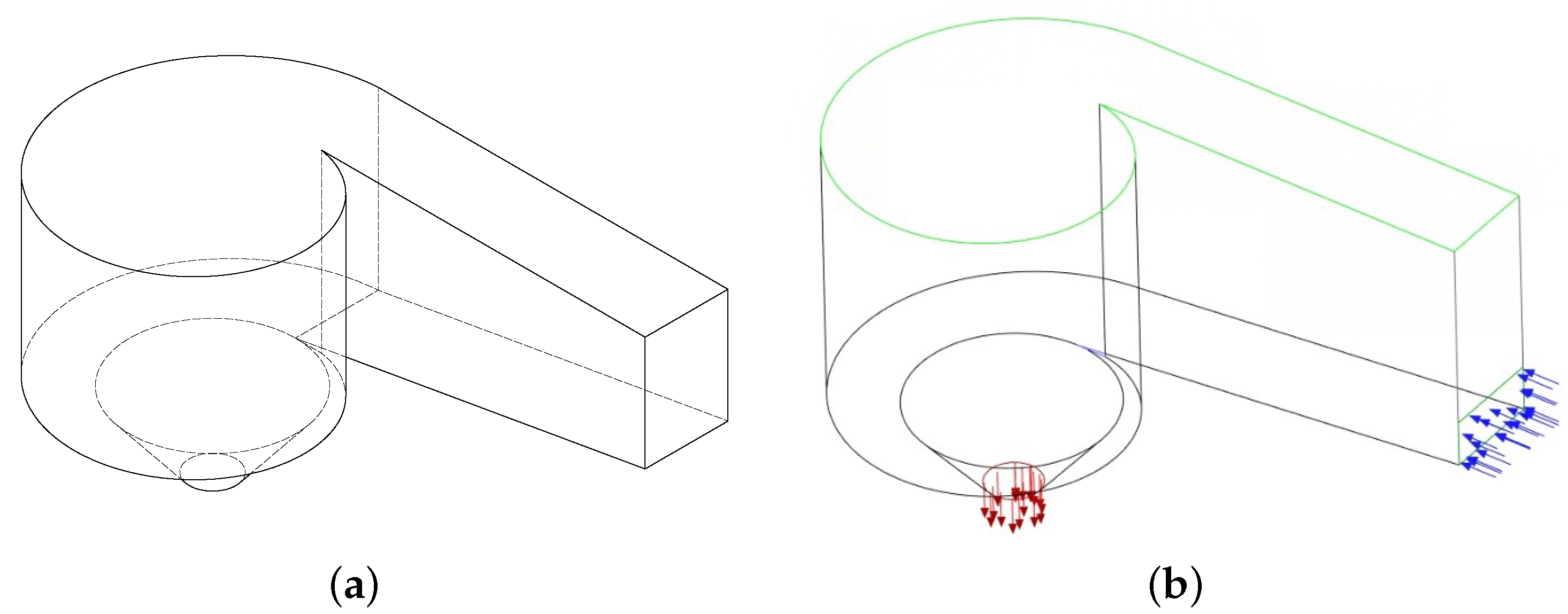
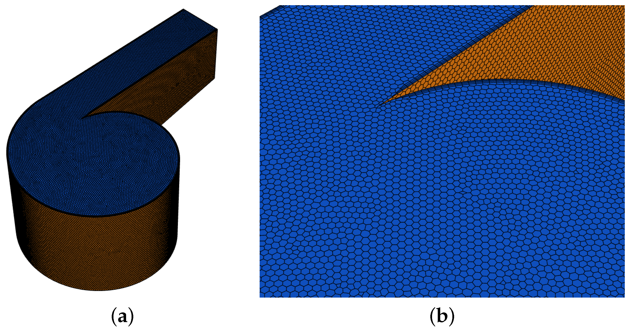
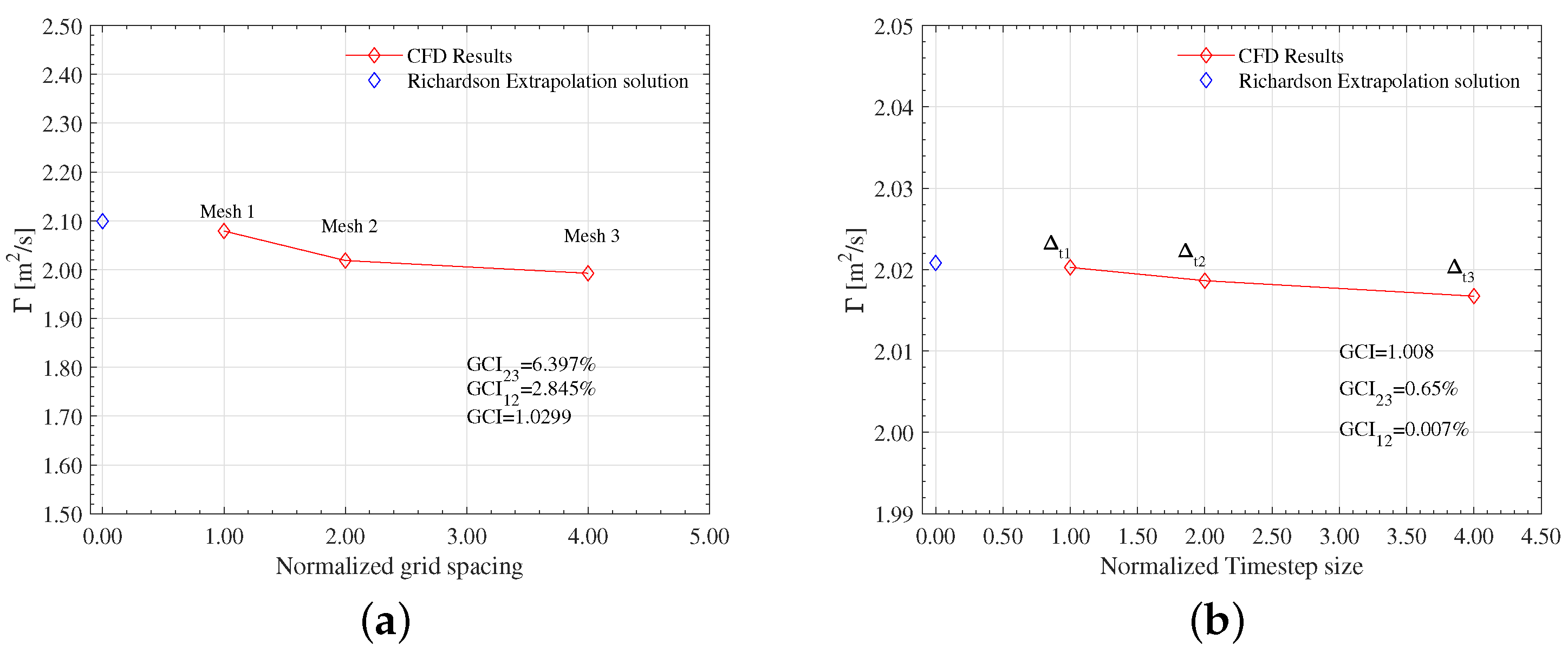
2.4. Numerical Simulation

CFD simulations have become an indispensable tool for analyzing and optimizing fluid systems, offering detailed insights into complex flow behaviors without the need for extensive physical experimentation [38,39]. This capability makes the tool particularly valuable for studying systems like GVTs, where understanding fluid circulation and phase interactions is critical to maximizing efficiency. The simulations were configured in ANSYS FLUENT 2023 R2. A transient simulation was conducted to capture the dynamic development of the fluid within the computational domain, with gravity acceleration activated to replicate real-world conditions. The inlet velocity V was set to 0.5 m/s for all models to maintain consistency across the experiments. However, the water flow rate (Q) varied between models due to differences in the inlet area, calculated as $Q=AV=H_c{W}_{c}V$, where $H_c$ and $W_c$ represent the height and width of the inlet channel, respectively. A pressure-based solver was employed for the simulations, as it is highly effective in capturing the complex behavior of fluid motion under varying flow conditions. The solution was initialized based on the inlet conditions, ensuring that the domain initially contained only air, allowing water to gradually fill the system.

The Unsteady Reynolds-Averaged Navier–Stokes (URANS) equations were solved using the coupled scheme for pressure–velocity coupling and second-order upwind discretization for improved accuracy. Since the turbine operated with two interacting fluids–air and water–the volume of fluid (VoF) method was chosen to track the interface between the phases. The inlet velocity was imposed as a boundary condition at the inlet channel, varying across simulations depending on the geometric characteristics of the study models. A relative pressure of 0 Pa was set at the discharge hole and upper surfaces to represent atmospheric conditions. The computational domain and boundary conditions are illustrated in Figure 3.

To model turbulence effects, the k-epsilon RNG turbulence model was employed due to its improved accuracy in capturing turbulent flows with moderate to high Reynolds numbers. This model is widely used in engineering applications as it provides a good balance between accuracy and computational cost, particularly in free-surface and shear-dominated flows [19,27]. Compared to the standard k-epsilon model, the RNG (Renormalization Group) variant offers better performance in flows with a strong streamline curvature, rotational effects, and rapid strain rates, making it more suitable for the present study. Additionally, the RNG formulation includes a modified dissipation term, enhancing its capability to predict flow separation and recirculation zones more accurately while maintaining numerical stability.

In this study, standard wall functions were applied to model near-wall turbulence, ensuring a proper representation of the velocity profile within the boundary layer. Standard wall functions are semi-empirical models used in turbulence simulations to bridge the gap between the wall and the first computational cell, avoiding the need for excessive mesh refinement near solid boundaries. These functions assume that the flow near the wall follows a logarithmic velocity profile and are valid for $Y+$ values ranging from 30 to 300. In this case, the first computational cell near the wall was set to 0.0015 m, ensuring an appropriate resolution of the boundary layer effects.

The simulation was executed with a time step of 0.01 s and 5000 iterations to ensure complete fluid development and accurate results. The numerical simulations were performed on a high-performance computing (HPC) system equipped with 16 CPU cores and 64 GB of RAM (LENOVO ThinkStation P520, Intel Xeon W2145 @ 3.7 GHz). The computational solver was executed in parallel processing mode to optimize the simulation time and ensure efficient resource utilization. Figure 4 shows the final mesh configuration with zoomed-in views of selected region to illustrate mesh refinement.

Post-processing focused on evaluating circulation at the center of the cone. Since the obtained circulation data included contributions from both water and air phases, the percentage of water circulation was calculated to isolate the liquid-phase contribution.

To ensure the consistency and reliability of the results in the numerical simulations, it is essential to perform a rigorous spatial and temporal independence study [39]. This analysis ensures that, regardless of spatial conditions (such as mesh size and the number of nodes) or temporal conditions (such as time step size), the results remain invariant or as close as possible to one another [40]. For the spatial independence simulations, a high-quality structured mesh was generated using ANSYS Fluent and Meshing. The Poly-HexCore meshing technique—a hybrid topology combining polygonal (hexagonal) geometries with polyhedral structures—was employed [41]. This technique is widely used in CFD due to its ability to efficiently model complex geometries. Conducting spatial independence studies requires running numerous numerical simulations and analyzing a target or response variable. An effective methodology for comparing these simulations is Richardson extrapolation, which uses a simplification of Taylor series expansions to approximate derivatives, integrals, and differential equations through finite differences [42,43]. Applying Richardson extrapolation yields a convergence index that measures the degree of similarity between simulations, helping to identify the configuration that ensures mesh-independent results. To verify spatial independence, three meshes with the same computational domain were employed: coarse, medium, and fine. The fine mesh consisted of 1,285,156 elements, the medium mesh 674,428 elements, and the coarse mesh 350,516 elements. Circulation values of 2.07, 2.01, and 1.99 m²/s were obtained for the fine, medium, and coarse meshes, respectively. Using these values, the Grid Convergence Index (GCI) was calculated for the fine and coarse meshes to determine the convergence index (I), which should ideally be as close to 1 as possible [19,27]. In this case, the calculated convergence index was $I=$ 1.0299, indicating that spatial independence was achieved due to its proximity to 1.

In addition to the convergence index, the value corresponding to the behavior of a subsequent solution approaching zero is calculated using Richardson extrapolation. This calculation helps to determine the behavior of the solutions along a line, and the line is expected to converge toward the solution given by Richardson extrapolation. The results are presented in Figure 5. In Figure 5a, the blue diamond represents the Richardson-extrapolated solution for an infinitely refined mesh. Similarly, in Figure 5b, the blue diamond denotes the extrapolated solution for a time step tending to zero.

The final mesh used for the simulation exhibited an average skewness of 0.01446, an average aspect ratio of 2.13757, and an average orthogonal quality of 0.98554. These three characteristics are critical for ensuring the accuracy and stability of numerical simulations. A low skewness value indicates that the elements are close to an ideal shape, minimizing interpolation errors. It is stated that skewness ranging between 0.25 and 0.5 provides a good-quality meshing [44,45,46]. An aspect ratio close to 1 is desirable to prevent numerical diffusion, although values below 3 are generally acceptable for structured and unstructured grids in CFD applications [44,47]. Additionally, an orthogonal quality close to 1 ensures that the cell faces align properly with the flow, reducing discretization errors [46,48,49]. The values obtained in this study confirmed the high quality of the mesh, reinforcing the reliability of the numerical results.

Similar to the spatial independence study, a temporal independence analysis was conducted using the following time steps and normalized values: a fine step of 0.005 s (normalized value of 1) with a total circulation of 2.0202 m²/s, a medium step of 0.01 s (normalized value of 2) with a circulation of 2.018 m²/s, and a coarse step of 0.02 s (normalized value of 4) with a circulation of 2.0167 m²/s. The calculated convergence index for the temporal study was I = 1.0008, indicating that temporal independence was achieved.

2.5. Experimental Validation

The optimal geometric configuration of the inlet channel and discharge cone was fabricated at a laboratory scale, followed by an experimental performance evaluation. The tests were conducted in a hydraulic channel specifically designed for hydrokinetic turbine analysis, enabling the characterization of flow hydrodynamics, energy conversion efficiency, and associated hydraulic losses. The experimental setup has a reservoir, a centrifugal pump IHM 30A-15W-IE2 (Ignacio Gómez IHM, Medellín, Colombia), a feed tank, and a pipeline system; see Figure 6. The setup enables the testing of various GVT configurations.

The turbine includes an inlet channel and a discharge cone, all constructed from acrylic to allow for flow visualization and to facilitate the hydrodynamic analysis of the system. The vortex turbine is installed after the feed tank. The turbine is connected to the feed tank through flanges. The feed tank plays a critical role in reducing turbulence from the pump and ensuring a steady, laminar water flow into the turbine’s inlet channel. In these experiments, a runner was used, as shown in Figure 7, featuring six blades with an upper diameter of 388 mm, a lower diameter of 80 mm, and a height of 180 mm. The runner design was primarily based on the model proposed by Edirisinghe [23], which consists of a conical runner with straight blades. The runner was manufactured using 3D printing with PETG, while its shaft was made of stainless steel to ensure strength and durability. The 3D printing process was optimized to achieve high mechanical strength and dimensional accuracy. The 3D printing setup consisted of a 245 °C nozzle, an 80 °C heated bed, and a print speed of 60 mm/s. A 0.2 mm layer height was chosen for a good compromise between print quality and duration. The infill density was set to 55% with a grill pattern to enhance structural integrity while minimizing weight. Additionally, the print was performed with an enclosed chamber to reduce warping and improve layer adhesion. These parameters ensured the runner’s durability, precision, and performance in experimental conditions.

Water was drawn from the reservoir and directed into the feed tank of the GVT system. A variable frequency drive, linked to a PLC, regulated the pump’s operation, allowing for a precise adjustment of the water flow rate. To monitor the system’s circulating flow, a Siemens SITRANS FM MAG 5100 flow sensor (Siemens, Munich, Germany) was incorporated into the PLC and installed in the pipeline between the reservoir and the feed tank. This setup allowed for real-time mass flow measurements, enabling adjustments to the variable frequency drive to achieve the specified input conditions for the tests. The Siemens SITRANS FM MAG 5100 flow sensor had an accuracy of ±0.2% of the measured flow rate, ensuring reliable mass flow measurements.

The feed tank, filled from its base by a pump, overflowed due to the rising water level, spilling into the inlet channel and then draining into the discharge chamber. This process generated a vortex, directing the water back to the reservoir and creating the hydraulic conditions necessary for turbine operation. The turbine was positioned at the vortex’s core to ensure direct interaction with the induced flow. It was mounted on a vertical axis and connected to the measurement and control system for the precise monitoring of its rotational behavior. The turbine rotated freely during the stabilization phase to ensure the establishment of steady-state conditions prior to further testing.

A Pololu 4741 motor (Pololu Robotics and Electronics, Nevada, The United States) was used as a braking mechanism or an electric generator to counteract the rotational motion induced by the vortex. It rotated in the opposite direction of the vortex-induced turbine motion, providing resistance to the rotor. The braking process was performed in incremental steps until the turbine came to a complete stop, enabling controlled experimentation under varying resistance levels.

A Futek TRS 605 torque sensor (Futek, California, The United States) was attached between the braking motor and the turbine’s shaft. The sensor recorded the torque, power, and turbine’s speed. The Futek TRS 605 torque sensor had a non-linearity of ±0.2% and a repeatability of ±0.05% of the full-scale measurement, ensuring precise torque data. Additionally, a Futek IHH 500 display, connected to both the sensor and a personal computer, recorded and transmitted these measurements with an accuracy of ±0.005% of the reading. This high-precision configuration ensured accurate data acquisition, enabling detailed analysis and storage of the turbine’s performance characteristics. Figure 8 shows the runner, inlet channel, discharge cone, and measurement and control system.

Figure 9 presents the final experimental setup, showcasing the key components of the system. The image highlights the acrylic elements, the rotor, and the connection between the vortex turbine and the feeding tank.

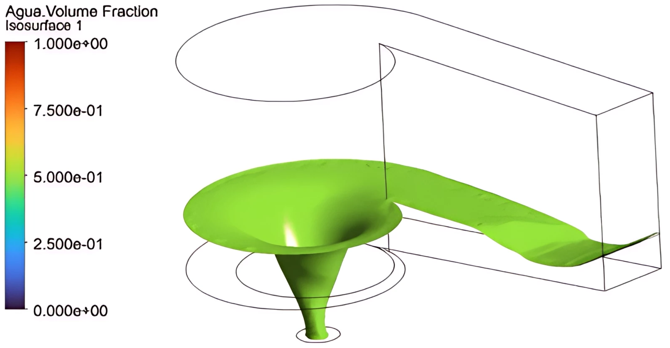
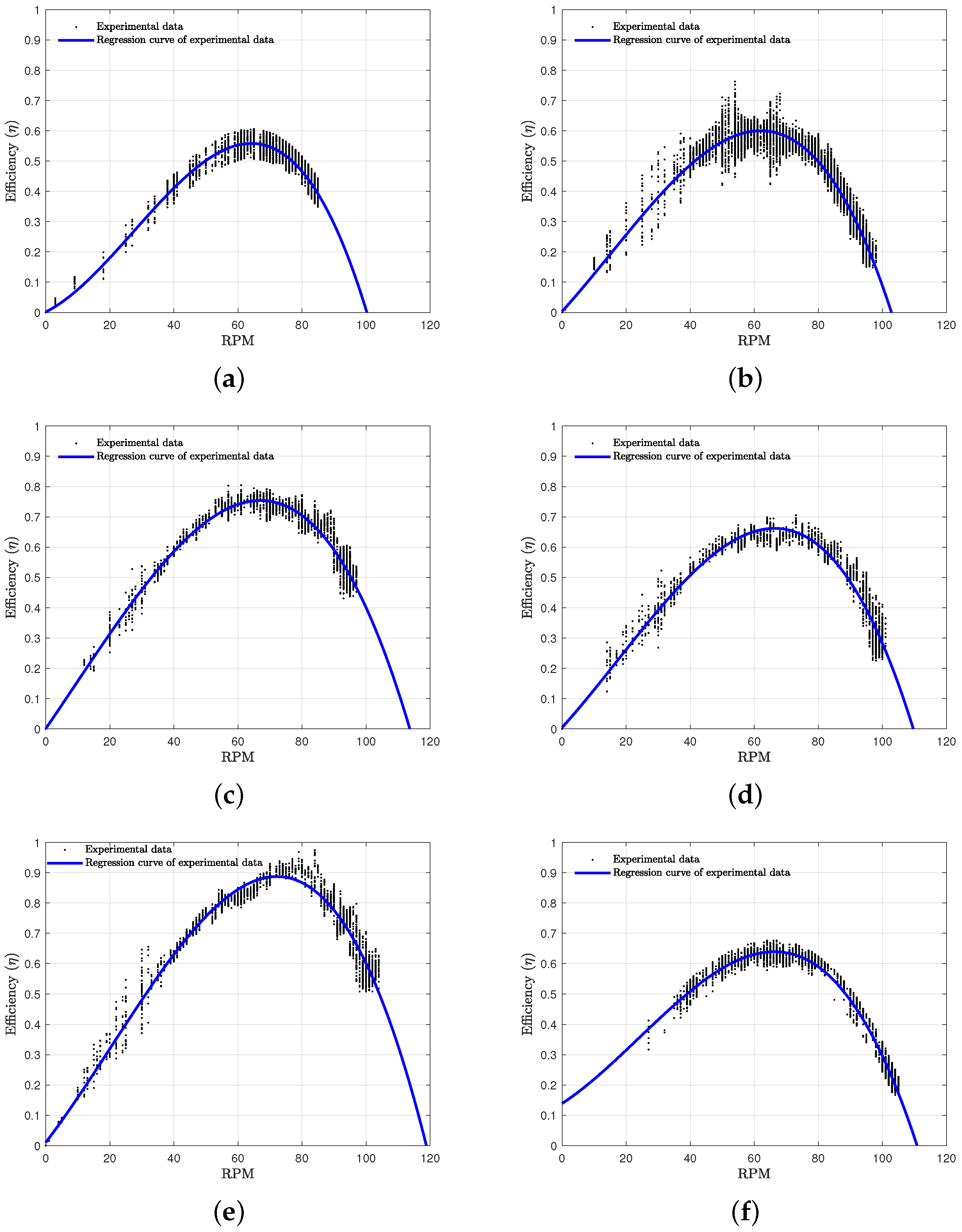
3. Results and Discussion

Upon completing the 27 simulations, the circulation results for the 3D models were obtained and are summarized in

Table 3. Numerical results.

Run	Γ [m2/s]	% Water Phase	Γwater [m2/s]	Mass Flow [kg/s]	% Deviation
1	2.2268	0.9065	2.0186	14.7205	2.18%
2	1.5919	0.9904	1.5909	14.7205	9.72%
3	1.6963	0.9707	1.6913	9.4211	4.93%
4	2.2411	0.8363	1.8742	9.4211	3.13%
5	1.6760	0.9956	1.6686	12.0708	5.78%
6	1.5975	0.9993	1.5964	14.7205	9.15%
7	1.7535	0.9980	1.7500	12.0708	5.37%
8	1.5569	0.9971	1.5524	9.4211	11.44%
9	1.7779	0.9972	1.7730	14.7205	9.88%
10	1.5777	0.9974	1.5736	9.4211	9.82%
11	2.2774	0.8645	1.9687	12.0708	5.43%
12	1.6919	0.9910	1.6887	12.0708	5.96%
13	2.2274	0.9048	1.9513	14.7205	5.05%
14	1.6752	0.9971	1.6706	9.4211	10.08%
15	1.7239	0.9967	1.7183	14.7205	9.83%
16	2.2419	0.8360	1.8742	9.4211	6.69%
17	2.3762	0.9051	2.1508	14.7205	4.52%
18	1.7750	0.9974	1.7704	12.0708	5.70%
19	2.3626	0.8384	1.9807	9.4211	6.22%
20	1.6316	0.9976	1.6277	9.4211	10.00%
21	2.2934	0.9152	2.0990	14.7205	4.87%
22	1.6154	0.9991	1.6140	14.7205	−0.83%
23	2.3357	0.8254	1.9280	9.4211	1.17%
24	1.5506	0.9975	1.5467	12.0708	0.14%
25	1.7532	0.9972	1.7484	12.0708	5.88%
26	1.7532	0.9972	1.7484	12.0708	5.88%
27	1.7532	0.9972	1.7484	12.0708	5.88%

. The table presents an overview of the results, including overall circulation, phase percentage, and liquid-phase circulation. Figure 10 illustrates the hydrodynamic behavior of water flowing through a vortex structure in a GVT. The vortex formation suggests a strong rotational flow and effective water circulation within the system. The sharp definition of the funnel indicates a well-developed vortex, essential for energy generation applications.

The models with the highest water-phase circulation are Model 17 (2.150835 m²/s) and Model 21 (2.09872 m²/s). Between the two models with the highest circulation, Runs 17 and 21, the only geometric difference is in the $H_c/D_{in}$ ratio. The values of $\alpha$, $W_c/D_{in}$, and $D_{out}/D_{in}$ remain the same, as well as the mass flow rate (14.7205 kg/s).

These models stand out as having superior circulation performance, which is crucial for the system’s energy generation efficiency. A higher circulation value is essential for maximizing the energy output because it enhances the velocity and angular momentum of the flow, which increases the turbine’s rotational speed. Additionally, it improves the interaction between the vortex flow and the turbine blades, thereby optimizing the transfer of energy. High circulation also ensures stable vortex formation, a crucial factor for a consistent and efficient turbine operation [18,27].

On the other hand, the models with the lowest circulation values are Model 24 (1.5467 m²/s) and Model 8 (1.5524 m²/s). These models exhibit reduced vortex strength, which may lead to a lower energy transfer efficiency. Lower circulation values can result in weaker vortex structures, reducing the velocity and angular momentum available for turbine operation. Consequently, this may impact the overall performance of the system, as a less stable vortex can hinder consistent energy generation and decrease turbine efficiency.

Figure 11 and Figure 12 show the water volume fraction for the models with higher and lower circulations, respectively. In both cases, subfigure (a) presents a cross-section at 50% of the cone height, while subfigure (b) displays a longitudinal section of the cone and inlet channel. The red region corresponds to the water within the vortex, while the blue areas represent air. Although a vortex forms in both cases, Figure 10 (Model 17) reveals the presence of an air core extending to the bottom of the cone, whereas in Figure 11 (Model 24), such a core is absent. This difference indicates that a higher circulation promotes air entrainment and the development of a more pronounced vortex structure. Additionally, the water volume fraction at 50% of the cone height differs significantly between the two models: for Model 17, it is 90.51%, whereas for Model 24, it is 99.75%. This variation highlights the influence of circulation intensity on the extent of air entrainment and the overall vortex dynamics within the system. The superiority of Model 17 in terms of circulation is due to a synergistic combination of its geometry, water fraction, and mass flow, which together create optimal conditions for a high circulation.

Based on the circulation data from each experiment, a second-order linear regression model (Equation (4)) was created. An ANOVA test was also run in RStudio 2024.12.0+467 to see how much the different factors affected circulation. This analysis generated p-values, which are presented in

Table 4. Analysis of variance (ANOVA) results.

Term	Effect	Df	SS	MS	F	P
$\alpha$	$-2.231\times {10}^{-1}$	1	0.0194	0.0194	5.831	0.03263
$D_{out}/D_{in}$	$-5.208$	1	0.5903	0.5903	176.976	$1.52\times {10}^{-8}$
$H_c/D_{in}$	$-1.758$	1	0.0052	0.0052	1.569	0.2342
$W_c/D_{in}$	$1.599$	1	0.0359	0.0359	10.760	0.00658
${\alpha }^2$	$-1.076\times {10}^{-2}$	1	0.0435	0.0435	13.027	0.00358
${(D_{out}/D_{in})}^2$	$1.283\times {10}^1$	1	0.0157	0.0157	4.693	0.05112
${(H_c/D_{in})}^2$	$7.328\times {10}^{-1}$	1	0.0006	0.0006	0.173	0.68485
${(W_c/D_{in})}^2$	$-4.057$	1	0.0028	0.0028	0.833	0.37945
$\alpha (D_{out}/D_{in})$	$1.019\times {10}^{-1}$	1	0.0037	0.0037	1.121	0.31055
$\alpha (H_c/D_{in})$	$2.354\times {10}^{-2}$	1	0.0011	0.0011	0.345	0.56802
$\alpha (W_c/D_{in})$	$1.846\times {10}^{-1}$	1	0.0177	0.0177	5.298	0.04008
$(D_{out}/D_{in})(H_c/D_{in})$	$1.073\times {10}^{-1}$	1	0	0	0.010	0.92169
$(D_{out}/D_{in})(W_c/D_{in})$	$3.446$	1	0.0087	0.0087	2.597	0.13306
$(H_c/D_{in})(W_c/D_{in})$	$3.204\times {10}^{-2}$	1	0	0	0.001	0.97191
Residuals	-	12	0.04	0.0033	-	-
$R^2$	0.9871	-	-	-	-	-
Adjusted $R^2$	0.9777	-	-	-	-	-

along with the coefficients of determination (R² and adjusted R²) obtained from the model. These coefficients indicate the percentage of the response variable’s variance accounted for by the model and should consistently be greater than 0.8 [50,51].

When examining p-values in Table 4 under a significance level of 0.05, it is evident that the term with the greatest impact on circulation is the ratio between the outlet channel diameter and the inlet channel diameter ($D_{out}/D_{in}$), with a p-value of $1.52\times {10}^{-8}$. The terms contributing the least to circulation variation are, first, the interaction between $H_c/D_{in}$ and $W_c/D_{in}$, followed by the interaction between $D_{out}/D_{in}$ and $H_c/D_{in}$.

The model’s overall p-value is $1.246\times {10}^{-5}$, verifying that the regression model is statistically significant and accurately represents the relationship between the experimental variables and circulation behavior. The residuals have a sum of squares of 0.04, indicating that the unexplained variance is relatively low. The R² value of 0.9871 indicates that 98.71% of the variance in circulation is explained by the model. The adjusted R² of 0.9777 confirms the model’s robustness even after accounting for the number of predictors.

Equation (5) represents the final regression model.

Along with R-squared and p-value, the model validation requires checking that the regression model meets statistical assumptions and fits the CFD data. This involves residual analysis (the difference between observed and predicted circulation values) [37,52,53]. Specifically, it is essential to validate the normality, independence, and constant variance of the residuals. If these analysis are not met, the regression model lacks statistical validity, potentially leading to biased predictions, unreliable confidence intervals, and misleading conclusions.

In regression modeling, assessing the normality of residuals is crucial to ensure that the error terms follow a normal distribution [53,54]. This assumption is first verified graphically by examining the frequency distribution (Figure 13a), where the histogram bars are expected to align with the normality line (red line). Following this, the normal probability plot (Figure 13b) is inspected, where points should closely follow the red line, indicating normality in the residuals. To reinforce these visual checks, numerical tests were conducted, as shown in

Table 5. Normality test results.

Test Name	p-Value	Test Statistic
Shapiro–Francia Test	0.1715	0.9484
Anderson–Darling Test	0.2890	0.4417
Shapiro–Wilk Test	0.2039	0.9491
Cramer–Von Mises Test	0.4486	0.0544
Jarque–Bera Test	0.5027	1.3757
KS Lilliefors Modification	0.2000	0.1114
KS Limiting Form	0.8907	0.5791
KS Marsaglia Method	0.8543	0.5791

. The table reveals that all p-values from the tests exceeded the threshold of 0.05, leading to the conclusion that the residuals conformed to a normal distribution.

$$\begin{array}{cc}\hfill \Gamma =& 3.539-2.231\times {10}^{-1}\alpha -5.208\left({\displaystyle \frac{D_{out}}{D_{in}}}\right)-1.758\left({\displaystyle \frac{H_c}{D_{in}}}\right)+1.599\left({\displaystyle \frac{W_c}{D_{in}}}\right)\hfill \\ \hfill & +1.019\times {10}^{-1}\alpha \left({\displaystyle \frac{D_{out}}{D_{in}}}\right)+2.354\times {10}^{-2}\alpha \left({\displaystyle \frac{H_c}{D_{in}}}\right)+1.846\times {10}^{-1}\alpha \left({\displaystyle \frac{W_c}{D_{in}}}\right)\hfill \\ \hfill & +1.073\times {10}^{-1}\left({\displaystyle \frac{D_{out}}{D_{in}}}\right)\left({\displaystyle \frac{H_c}{D_{in}}}\right)+3.446\left({\displaystyle \frac{D_{out}}{D_{in}}}\right)\left({\displaystyle \frac{W_c}{D_{in}}}\right)\hfill \\ \hfill & +3.204\times {10}^{-2}\left({\displaystyle \frac{H_c}{D_{in}}}\right)\left({\displaystyle \frac{W_c}{D_{in}}}\right)-1.076\times {10}^{-2}{\alpha }^2+1.283\times {10}^1{\left({\displaystyle \frac{D_{out}}{D_{in}}}\right)}^2\hfill \\ \hfill & +7.328\times {10}^{-1}{\left({\displaystyle \frac{H_c}{D_{in}}}\right)}^2-4.057{\left({\displaystyle \frac{W_c}{D_{in}}}\right)}^2\hfill \end{array}$$

(5)

The independence of residuals, indicating no autocorrelation, was another essential assumption [55]. This was verified using the Durbin–Watson test [56], which yielded a p-value of 0.9459. Such a high p-value confirms that the residuals were independent and randomly distributed. Finally, the assumption of constant variance was tested using the Breusch–Pagan test [57,58], which returned a p-value of 0.1349. This result confirms that the variance of the residuals was homogeneous, indicating no signs of heteroscedasticity. Together, these tests validate the model’s adherence to key regression assumptions. Once the previous model was validated, it was used to predict the optimal design—defined as the design that maximizes circulation. The response surfaces generated by the interactions between pairs of factors are illustrated in Figure 14. Each subfigure represents the variation of circulation ($\Gamma$) as a function of two independent variables, allowing for a comprehensive evaluation of their combined effect. In general, the response surfaces reveal that higher circulation values are associated with specific parameter combinations, highlighting the importance of optimizing these variables to enhance vortex strength. Notably, in subfigures (a), (c), and (e), circulation increases with larger dimensionless diameters and angles, suggesting that these parameters play a crucial role in improving the vortex structure. Conversely, in subfigures (b), (d), and (f), circulation appears less sensitive to variations in height ratios and width ratios, indicating a relatively smaller influence on vortex performance.

To improve result readability, contour plots corresponding to the response surfaces are included in Figure 15, providing a clearer visualization of the trends and interactions between the studied parameters.

From Figure 15a, the highest circulation values occur at higher values of $D_{out}/D_{in}$ and $\alpha$. From Figure 15b, the highest circulation is achieved when $H_c$ is above 1.35 and $\alpha$ exceeds 9°. In Figure 15c, the combination of a higher $W_c/D_{in}$ and a larger $\alpha$ results in maximum circulation. In Figure 15d, the highest circulation is observed when $H_c/D_{in}$ and $D_{out}/D_{in}$ are both high. In Figure 15e, the optimal condition for circulation occurs when $W_c/D_{in}$ and $D_{out}/D_{in}$ are maximized. Finally, in Figure 15f, the highest circulation values are achieved when $H_c/D_{in}$ is high and $W_c/D_{in}$ is low.

The determination of ideal parameter values for each factor was limited to the initially established design space, taking into account the constraints imposed by the maximum allowable diameters due to the discharge chamber walls and the feasibility of constructing the subsequent experimental model. The optimal model identified by the software corresponds to Model 17, which is presented in Table 3. This model features an $\alpha$ of 10°, the highest value considered; a $D_{out}/D_{in}$ of 0.280, which represents the upper limit for this factor; a $H_c/D_{in}$ of 1.06, corresponding to the lower bound of this variable; and a width ratio $W_c/D_{in}$ of 0.50, the maximum value allowed within the design space.

Once the regression model was validated, and with the optimal model and fabricated rotor ready, experimentation with the turbine proceeded. From the experimental measurements, the efficiency curve ($\eta$) was plotted as a function of the rotor’s angular velocity using the rotational speed and delivered torque data. These measurements range from the turbine spinning freely at its maximum speed to the point where it comes to a complete stop.

Table 6. Flow rate and available power for different scenarios.

Flow Rate [L/s]	Flow Rate [m3/s]	Power [W]
3.3	0.0033	11.4114
5.6	0.0056	19.3649
7.6	0.0076	26.2809
8.3	0.0083	28.7016
8.9	0.0089	30.7764
9.4	0.0094	32.5054

presents the flow rate and available power data for each of the experimentally analyzed cases, which were used to calculate the efficiency for each scenario.

The curves presented in Figure 16 show the results obtained for each scenario, for flow rates ranging from 3.3 to 9.4 L/s. In Figure 16a, efficiency increases gradually with rotational speed, peaking at around 70 RPM before declining, indicating an optimal speed for maximum performance. A similar trend is observed in Figure 16b, although the peak efficiency is slightly higher and occurs between 70 and 80 RPM. Figure 16c presents a smoother, more pronounced efficiency curve, with a peak at approximately 75 RPM, suggesting enhanced performance at higher flow rates. In Figure 16d, the peak efficiency is observed near 80 RPM, with a broader curve indicating greater stability across a wider range of rotational speeds. Figure 16e shows a well-defined curve peaking at around 85 to 90 RPM, reflecting a higher overall efficiency and better utilization of increased flow. Notably, the highest efficiency of all scenarios, 0.8770, was achieved in this case at 71.54 RPM with a flow rate of 8.9 L/s. Finally, in Figure 16f, the highest flow rate produces a broader efficiency curve, peaking at 85 to 90 RPM. Despite minor fluctuations, the curve suggests stable performance over a wide RPM range.

4. Conclusions

Access to electricity in remote, non-interconnected regions remains a global challenge, reflecting not only technical and economic barriers but also deep social inequalities. This study highlights the urgent need to rethink traditional energy solutions and promote technologies that are sustainable, accessible, and adapted to the unique characteristics of these regions. Gravitational vortex turbines have emerged as a promising alternative by harnessing small water flows without requiring large-scale infrastructure. Their simple and modular design allows for implementation in rural communities with limited resources, providing clean and efficient energy that respects local ecosystems. The impact of this technology extends beyond technical performance. Socially, electricity transforms community dynamics by promoting economic opportunities and improving quality of life. However, the success of these projects depends not only on technology but also on community involvement in every phase—from design to implementation—to ensure that proposed solutions address real needs and respect cultural contexts. The CFD simulation analyses revealed that Design 17 exhibited the highest fluid circulation, making it the most optimal model. The validation of the experimental design, based on residual analysis, confirmed that accounting for impeller inertia is crucial to achieving accurate models that closely match experimental results. The statistical analysis confirmed that the ratio between discharge and inlet diameters ($D_{out}/D_{in}$) is the most influential design factor on fluid circulation. The optimized design for the system had an $\alpha$ factor of 10°, a $D_{out}/D_{in}$ ratio of 0.28, an $H_c/D_{in}$ ratio of 1.06, and a $W_c/D_{in}$ ratio of 0.5, which was validated through variance analysis with a minimal prediction error (1.542%). The experimental results also indicated that a flow rate of 0.0089 m³/s maximized system efficiency, achieving a peak value of 0.8770 at 71.54 RPM. Operating at higher speeds led to a decline in efficiency, highlighting the importance of maintaining the system at its optimal efficiency point to improve overall performance and maximize power generation.

Despite the promising results, this study acknowledges several limitations. First, laboratory-scale experiments inherently simplify real-world conditions. Factors such as turbulence, sediment transport, and long-term structural wear were not accounted for in the controlled test environment but could significantly impact turbine performance in natural water bodies. Additionally, while CFD simulations provide valuable insights, they relied on assumptions and boundary conditions that may not fully capture the complexity of real-world hydrodynamic interactions. Another limitation is the scale of implementation. While gravitational vortex turbines offer an efficient and sustainable solution for small-scale decentralized energy generation, their power output remains limited compared to conventional hydropower systems. The applicability of the optimized design to full-scale installations requires further validation through field testing under varying environmental conditions. Future research should focus on long-term performance monitoring in real settings to assess durability, efficiency, and maintenance requirements.

Moreover, economic and regulatory challenges must be considered. The feasibility of widespread adoption depends on cost-effectiveness, ease of deployment, and alignment with local energy policies. Community acceptance and participation are also critical, as social factors influence the long-term sustainability of the technology. Addressing these limitations through pilot projects in real-world conditions will be essential to bridging the gap between laboratory findings and practical implementation. Future work should also explore hybrid energy integration and adaptive design modifications to enhance the robustness and scalability of gravitational vortex turbines for rural electrification.

References

1. Jie, H.; Khan, I.; Alharthi, M.; Zafar, M.W.; Saeed, A. Sustainable energy policy, socio-economic development, and ecological footprint: The economic significance of natural resources, population growth, and industrial development. Util. Policy 2023, 81, 101490. [Google Scholar] [CrossRef]
2. Dodds, S. Economic growth and human well-being. In Human Ecology, Human Economy; Routledge: Oxfordshire, UK, 2020; pp. 98–124. [Google Scholar]
3. Ghasemian, S.; Faridzad, A.; Abbaszadeh, P.; Taklif, A.; Ghasemi, A.; Hafezi, R. An overview of global energy scenarios by 2040: Identifying the driving forces using cross-impact analysis method. Int. J. Environ. Sci. Technol. 2020, 21, 7749–7772. [Google Scholar] [CrossRef]
4. Molotoks, A.; Smith, P.; Dawson, T.P. Impacts of land use, population, and climate change on global food security. Food Energy Secur. 2021, 10, e261. [Google Scholar] [CrossRef]
5. Bin Rahman, A.R.; Zhang, J. Trends in rice research: 2030 and beyond. Food Energy Secur. 2023, 12, e390. [Google Scholar] [CrossRef]
6. Hosan, S.; Karmaker, S.C.; Rahman, M.M.; Chapman, A.J.; Saha, B.B. Dynamic links among the demographic dividend, digitalization, energy intensity and sustainable economic growth: Empirical evidence from emerging economies. J. Clean. Prod. 2022, 330, 129858. [Google Scholar] [CrossRef]
7. Ahmad, T.; Zhang, D. A critical review of comparative global historical energy consumption and future demand: The story told so far. Energy Rep. 2020, 6, 1973–1991. [Google Scholar] [CrossRef]
8. Jenkins, R. How China Is Reshaping the Global Economy: Development Impacts in Africa and Latin America; Oxford University Press: Oxford, UK, 2022. [Google Scholar]
9. United Nations Department of Economic and Social Affairs; Hertog, S.; Gerland, P.; Wilmoth, J. India overtakes China as the world’s most populous country. In UN Department of Economic and Social Affairs (DESA) Policy Briefs; UN Department of Economic and Social Affairs: New York, NY, USA, 2023. [Google Scholar]
10. Echendu, A.J.; Okafor, P.C.C. Smart city technology: A potential solution to Africa’s growing population and rapid urbanization? Dev. Stud. Res. 2021, 8, 82–93. [Google Scholar] [CrossRef]
11. Grinin, L.; Korotayev, A. Africa: The continent of the future. Challenges and opportunities. In Reconsidering the Limits to Growth: A Report to the Russian Association of the Club of Rome; Springer: Berlin/Heidelberg, Germany, 2023; pp. 225–238. [Google Scholar]
12. Kabeyi, M.J.B.; Olanrewaju, O.A. Sustainable energy transition for renewable and low carbon grid electricity generation and supply. Front. Energy Res. 2022, 9, 743114. [Google Scholar] [CrossRef]
13. Pandey, M.; Gusain, D. Energy: Present and Future Demands. In Advanced Nanocatalysts for Biodiesel Production; CRC Press: Boca Raton, FL, USA, 2022; pp. 1–16. [Google Scholar]
14. Breyer, C.; Khalili, S.; Bogdanov, D.; Ram, M.; Oyewo, A.S.; Aghahosseini, A.; Gulagi, A.; Solomon, A.; Keiner, D.; Lopez, G.; et al. On the history and future of 100% renewable energy systems research. IEEE Access 2022, 10, 78176–78218. [Google Scholar] [CrossRef]
15. Strielkowski, W.; Civín, L.; Tarkhanova, E.; Tvaronavičienė, M.; Petrenko, Y. Renewable energy in the sustainable development of electrical power sector: A review. Energies 2021, 14, 8240. [Google Scholar] [CrossRef]
16. Rahman, A.; Farrok, O.; Haque, M.M. Environmental impact of renewable energy source based electrical power plants: Solar, wind, hydroelectric, biomass, geothermal, tidal, ocean, and osmotic. Renew. Sustain. Energy Rev. 2022, 161, 112279. [Google Scholar] [CrossRef]
17. Schillinger, M.; Weigt, H.; Hirsch, P.E. Environmental flows or economic woes—Hydropower under global energy market changes. PLoS ONE 2020, 15, e0236730. [Google Scholar] [CrossRef] [PubMed]
18. Maika, N.; Lin, W.; Khatamifar, M. A review of gravitational water vortex hydro turbine systems for hydropower generation. Energies 2023, 16, 5394. [Google Scholar] [CrossRef]
19. Velásquez, L.; Posada, A.; Chica, E. Optimization of the basin and inlet channel of a gravitational water vortex hydraulic turbine using the response surface methodology. Renew. Energy 2022, 187, 508–521. [Google Scholar] [CrossRef]
20. Velásquez, L.; Rubio-Clemente, A.; Chica, E. Numerical and Experimental Analysis of Vortex Profiles in Gravitational Water Vortex Hydraulic Turbines. Energies 2024, 17, 3543. [Google Scholar] [CrossRef]
21. Aziz, M.Q.A.; Idris, J.; Abdullah, M.F. Experimental study on enclosed gravitational water vortex turbine (GWVT) producing optimum power output for energy production. J. Adv. Res. Fluid Mech. Therm. Sci. 2022, 95, 146–158. [Google Scholar]
22. Velásquez, L.; Chica, E.; Posada, J. Advances in the Development of Gravitational Water Vortex Hydraulic Turbines. J. Eng. Sci. Technol. Rev. 2021, 14, 1–14. [Google Scholar] [CrossRef]
23. Edirisinghe, D.S.; Yang, H.S.; Gunawardane, S.; Lee, Y.H. Enhancing the performance of gravitational water vortex turbine by flow simulation analysis. Renew. Energy 2022, 194, 163–180. [Google Scholar] [CrossRef]
24. Jiang, Y.; Raji, A.P.; Raja, V.; Wang, F.; AL-bonsrulah, H.A.; Murugesan, R.; Ranganathan, S. Multi–disciplinary optimizations of small-scale gravitational vortex hydropower (SGVHP) system through computational hydrodynamic and hydro–structural analyses. Sustainability 2022, 14, 727. [Google Scholar] [CrossRef]
25. Betancour, J.; Romero-Menco, F.; Velásquez, L.; Rubio-Clemente, A.; Chica, E. Design and optimization of a runner for a gravitational vortex turbine using the response surface methodology and experimental tests. Renew. Energy 2023, 210, 306–320. [Google Scholar] [CrossRef]
26. Mobeen, M.; Jaweed, S.; Abdullah, A.; Rasheed, S.; Masud, M. Parametric Optimization of Gravitational Water Vortex Turbines for Enhanced Torque Generation. Eng. Proc. 2023, 45, 3. [Google Scholar] [CrossRef]
27. Velásquez, L.; Posada, A.; Chica, E. Surrogate modeling method for multi-objective optimization of the inlet channel and the basin of a gravitational water vortex hydraulic turbine. Appl. Energy 2023, 330, 120357. [Google Scholar] [CrossRef]
28. Septyaningrum, E.; Hantoro, R.; Mouti, N.K.; Rahayu, W.R.; Banta Cut, S. Gravitational Vortex Water Turbine (GVWT) conical basin design: The effects of cone angle and outlet diameter on vortex characteristics. J. Mech. Eng. (JMechE) 2024, 21, 177–198. [Google Scholar]
29. Spichal, L. Gielis transformation of the Archimedean spiral. Kragujev. J. Math. 2025, 49, 431–442. [Google Scholar] [CrossRef]
30. Lamidi, S.; Olaleye, N.; Bankole, Y.; Obalola, A.; Aribike, E.; Adigun, I. Applications of Response Surface Methodology (RSM) in Product Design, Development, and Process Optimization; IntechOpen: Rijeka, Croatia, 2022. [Google Scholar]
31. Hadiyat, M.A.; Sopha, B.M.; Wibowo, B.S. Response surface methodology using observational data: A systematic literature review. Appl. Sci. 2022, 12, 10663. [Google Scholar] [CrossRef]
32. Szpisják-Gulyás, N.; Al-Tayawi, A.N.; Horváth, Z.H.; László, Z.; Kertész, S.; Hodúr, C. Methods for experimental design, central composite design and the Box–Behnken design, to optimise operational parameters: A review. Acta Aliment. 2023, 52, 521–537. [Google Scholar] [CrossRef]
33. Tamandani, M.; Hashemi, S.H. Central composite design (CCD) and Box-Behnken design (BBD) for the optimization of a molecularly imprinted polymer (MIP) based pipette tip micro-solid phase extraction (SPE) for the spectrophotometric determination of chlorpyrifos in food and juice. Anal. Lett. 2022, 55, 2394–2408. [Google Scholar] [CrossRef]
34. Rigdon, S.E.; Englert, B.R.; Lawson, I.A.; Borror, C.M.; Montgomery, D.C.; Pan, R. Experiments for reliability achievement. Qual. Eng. 2012, 25, 54–72. [Google Scholar] [CrossRef]
35. Montgomery, D.C.; Runger, G.C. Applied Statistics and Probability for Engineers; John Wiley & Sons: New York, NY, USA, 2010. [Google Scholar]
36. Bhattacharya, S. Central composite design for response surface methodology and its application in pharmacy. In Response Surface Methodology in Engineering Science; IntechOpen: Rijeka, Croatia, 2021. [Google Scholar]
37. Montgomery, D.C.; Peck, E.A.; Vining, G.G. Introduction to Linear Regression Analysis; John Wiley & Sons: New York, NY, USA, 2021. [Google Scholar]
38. bin Ismail, H.; Nguyen, M.Q. A Comparative Analysis of Efficiency in Fluid Dynamic Devices: Experimental and Computational Approaches. Q. J. Emerg. Technol. Innov. 2023, 8, 85–102. [Google Scholar]
39. Tu, J.; Yeoh, G.H.; Liu, C.; Tao, Y. Computational Fluid Dynamics: A Practical Approach; Elsevier: Amsterdam, The Netherlands, 2023. [Google Scholar]
40. Urrego-Pabón, J.; Mercado, J.; Obando-Vega, F.; Rubio-Clemente, A.; Chica, E. Numerical and experimental study of several passive wave absorber behavior in a wave channel. Results Eng. 2024, 23, 102455. [Google Scholar] [CrossRef]
41. Rajashekaraiah, T.; Panigrahi, S.P.; Sanjai, G.S.; Dulabhai, H.P.; Vijaykumar, V. Investigating Various Meshing Techniques in Computational Fluid Dynamics (CFD) for their Impact on Heat Transfer Parameters of Fins. J. Mines Met. Fuels 2025, 73, 117–128. [Google Scholar] [CrossRef]
42. Long, G.; Liu, L.B.; Huang, Z. Richardson extrapolation method on an adaptive grid for singularly perturbed Volterra integro-differential equations. Numer. Funct. Anal. Optim. 2021, 42, 739–757. [Google Scholar] [CrossRef]
43. Soori, Z.; Aminataei, A. Numerical solution of space fractional diffusion equation by spline method combined with Richardson extrapolation. Comput. Appl. Math. 2020, 39, 136. [Google Scholar] [CrossRef]
44. ANSYS, Inc. ANSYS Fluent 14.5 User’s Guide; ANSYS, Inc.: Canonsburg, PA, USA, 2012. [Google Scholar]
45. Al-Dabbagh, M.A.; Yuce, M.I. Simulation and comparison of helical and straight-bladed hydrokinetic turbines. Int. J. Renew. Energy Res. 2018, 8, 504–513. [Google Scholar]
46. Antar, E.; Elkhoury, M. Parametric sizing optimization process of a casing for a Savonius Vertical Axis Wind Turbine. Renew. Energy 2019, 136, 127–138. [Google Scholar] [CrossRef]
47. Zadorozhna, D.B.; Benavides, O.; Grajeda, J.S.; Ramirez, S.F.; de la Cruz May, L. A parametric study of the effect of leading edge spherical tubercle amplitudes on the aerodynamic performance of a 2D wind turbine airfoil at low Reynolds numbers using computational fluid dynamics. Energy Rep. 2021, 7, 4184–4196. [Google Scholar] [CrossRef]
48. Mereu, R.; Passoni, S.; Inzoli, F. Scale-resolving CFD modeling of a thick wind turbine airfoil with application of vortex generators: Validation and sensitivity analyses. Energy 2019, 187, 115969. [Google Scholar] [CrossRef]
49. Al-quraishi, B.A.J.; Aboaltabooq, M.H.K.; AL-Fatlwe, F.M.K. A simulation investigation the performance of a small scale Elliptical Savonius wind turbine with twisting blades and sloping ends plates. Period. Eng. Nat. Sci. (PEN) 2022, 10, 376–386. [Google Scholar] [CrossRef]
50. Elmousalami, H.H. Artificial intelligence and parametric construction cost estimate modeling: State-of-the-art review. J. Constr. Eng. Manag. 2020, 146, 03119008. [Google Scholar] [CrossRef]
51. Öztürk, B. Time Series Models for Revenue Forecasting in the Semiconductor Industry: A Case Study of ASML. Master’s Thesis, Tilburg School of Economics and Management, Tilburg, The Netherlands, 2024. [Google Scholar]
52. Roustaei, N. Application and interpretation of linear-regression analysis. Med. Hypothesis Discov. Innov. Ophthalmol. 2024, 13, 151. [Google Scholar] [CrossRef]
53. Pardoe, I. Applied Regression Modeling; John Wiley & Sons: New York, NY, USA, 2020. [Google Scholar]
54. Hernandez, H. Testing for normality: What is the best method. ForsChem Res. Rep. 2021, 6, 1–38. [Google Scholar]
55. Mignon, V. Heteroskedasticity and Autocorrelation of Errors. In Principles of Econometrics: Theory and Applications; Springer: Berlin/Heidelberg, Germany, 2024; pp. 171–221. [Google Scholar]
56. Shah, M.A.A.; Ozel, G.; Chesneau, C.; Mohsin, M.; Jamal, F.; Bhatti, M.F. A statistical study of the determinants of rice crop production in Pakistan. Pak. J. Agric. Res. 2020, 33, 97. [Google Scholar] [CrossRef]
57. Đalić, I.; Terzić, S. Violation of the assumption of homoscedasticity and detection of heteroscedasticity. Decis. Mak. Appl. Manag. Eng. 2021, 4, 1–18. [Google Scholar] [CrossRef]
58. Uyanto, S.S. Monte Carlo power comparison of seven most commonly used heteroscedasticity tests. Commun.-Stat. Comput. 2022, 51, 2065–2082. [Google Scholar] [CrossRef]
Figure 1. Schematic representation of the Archimedean spiral and its geometric parameters.
Processes 13 01533 g001
Figure 2. The selected geometric parameters for the optimization.
Processes 13 01533 g002
Figure 3. Computational model of the gravitational vortex turbine: (a) defined computational domain, (b) boundary conditions, where blue arrows represent the inlet velocity and red arrows represent the outlet pressure.
Processes 13 01533 g003
Figure 4. (a,b) Final mesh configuration with zoomed-in views of selected region to illustrate mesh refinement.
Processes 13 01533 g004
Figure 5. Grid and time step independence analysis using Richardson extrapolation: (a) grid independence study, (b) time step independence study.
Processes 13 01533 g005
Figure 6. Schematic representation of the experimental setup, including the feed tank, pipeline system, reservoir, centrifugal pump, and flow sensor.
Processes 13 01533 g006
Figure 7. Runner of the gravitational vortex turbine. (a) Technical drawing of the designed runner with dimensions and blade configuration. (b) 3D-model of the fabricated runner.
Processes 13 01533 g007
Figure 8. Runner, inlet channel, discharge cone, and measurement and control system.
Processes 13 01533 g008
Figure 9. Final experimental setup of the turbine system.
Processes 13 01533 g009
Figure 10. CFD simulation of the gravitational vortex flow. Visualization of the water volume fraction, illustrating the formation and structure of the vortex within the basin.
Processes 13 01533 g010
Figure 11. Water volume fraction for the model with a higher circulation (Run 17): (a) cross-section at 50% of the cone height, (b) longitudinal section of the cone and inlet channel.
Processes 13 01533 g011
Figure 12. Water volume fraction for the model with a lower circulations (Run 24): (a) cross-section at 50% of the cone height, (b) longitudinal section of the cone and inlet channel.
Processes 13 01533 g012
Figure 13. Normality test. (a) Frequency, (b) probability plot.
Processes 13 01533 g013
Figure 14. (af) Response surface results for the factors α , D o u t / D i n , H c / D i n , and W c / D i n .
Processes 13 01533 g014
Figure 15. (af) Contour plot for the factors α , D o u t / D i n , H c / D i n , and W c / D i n .
Processes 13 01533 g015
Figure 16. Efficiency vs. rotational speed curves across 6 different flow rates. (a) 3.3 L/s, (b) 5.6 L/s, (c) 7.6 L/s, (d) 8.3 L/s, (e) 8.9 L/s, and (f) 9.4 L/s.
Processes 13 01533 g016