Mathematical Model to Improve Energy Efficiency in Hammer Mills and Its Use in the Feed Industry: Analysis and Validation in a Case Study in Cuba

Abstract

The feed industry is characterized by high energy consumption during the grinding stage, where hammer mills can account for up to 50% of total electricity usage; furthermore, efficiency analyses are based only on the classical equations reported in the literature. In this context, the present theoretical-applied research aimed to improve the efficiency of a plant operating below its nominal capacity. To achieve this, a comprehensive mathematical model was developed, integrating power and grain disintegration equations while overcoming the limitations of classical comminution theories. The model incorporates key factors such as feed rate, moisture content, absorbed power and hammer wear. Additionally, specific correction factors for temperature ($K_t$) and mechanical degradation ($K_d$) were introduced to accurately represent real operating conditions. The study was based on extensive measurements of electrical current, power factor, energy consumption, particle size distribution and thermal variations under different load conditions. The statistical analysis, which included ANOVA, ANCOVA and multiple regressions, demonstrated a predictive accuracy of 98% (R²) and a pseudo-R² of 89%. This high correlation allowed for an 18% reduction in energy consumption equivalent to 4 kWh/t and up to a 30% improvement in particle size uniformity, surpassing typical factory performance. The findings highlight that integrating operational, thermodynamic and wear-related factors enhances the robustness of the model, promoting more reliable energy-management practices in hammer mills. Consequently, the results confirm that the developed model serves as a scientifically robust, efficient and applicable tool for improving energy efficiency and reducing environmental impacts in the agri-food industry.

1. Introduction

The growing global demand for animal feed for the agricultural sector, projected to reach a market value of more than USD 500 billion by 2030, has intensified production in feed mills, which poses significant challenges in terms of energy consumption and environmental sustainability [1,2]. These facilities face structural deficiencies in the efficient use of energy, with consumptions ranging from 15 to 50 kWh/t processed, depending on the equipment used, raw material characteristics and operating conditions [3,4]. This high energy consumption represents up to 30% of operating costs in some factories and contributes significantly to greenhouse gas emissions, with impacts estimated at 0.08 to 0.15 t CO₂/t processed [5,6].

Several studies have evaluated energy consumption in feed mills, identifying that the main equipment involved, such as mixers, pelletizers and conveying systems, contribute variably to energy demand. Mixers, for example, consume between 2 and 4 kWh/t, while pelletizers require between 5 and 7 kWh/t and conveying systems range between 1 and 2 kWh/t [7,8,9]. However, hammer mills stand out as the largest energy consumers, accounting for up to 50% of total mill consumption. These equipment items present energy values that vary between 8 and 30 kWh/t processed, depending on factors such as mill design, screen size, rotor speed and hammer wear [10,11,12,13].

Hammer mills are fundamental in the feed industry because of their critical role in particle size reduction. This process not only ensures uniform particle size, but also improves the digestibility of nutrients in animal diets and optimizes the subsequent stages of mixing and compaction [14,15,16]. However, the energy efficiency of this equipment is highly variable and is influenced by factors such as material density (ranging from 0.5 to 0.8 ${\mathrm{g}/\mathrm{cm}}^3$, rotor speed (1500 to 3000 rpm), screen design (2 to 6 mm openings) and material moisture (5% to 15%) [17,18,19,20]. It has been reported that hammer wear, when not properly managed, can increase energy consumption by 25%, resulting in an increase of up to 5 kWh/t processed [21,22,23].

Although mathematical models have been developed to analyze and optimize energy consumption in hammer mills, they have significant shortcomings. Classical theories, such as those of Bond, Rittinger and Kick, have been useful for correlating energy consumption with initial and final particle size. However, these theories assume ideal conditions and do not integrate dynamic variables such as hammer wear, fine particle accumulation on the screens and variations in material feed [24,25,26,27]. However, these classical formulations cannot account for the inherent complexity of industrial processes, as they do not take into account dynamic variables such as actual particle size distribution, equipment wear variability or thermal effects. In response, advanced models have been developed that integrate particle-level simulations using the discrete element method (DEM) and population balance models (PBMs), which allow more accurate predictions of process dynamics and the evolution of particle size distribution as a function of critical operational variables [28,29,30].

Additionally, approaches incorporating microhydrodynamic analysis and fractal techniques have enabled a more detailed description of the relationship between fragmentation energy and particle morphology, facilitating the optimization of energy consumption according to the specific characteristics of the material [31,32]. The combination of these methods not only enhances the accuracy of energy-consumption predictions but also offers the potential for implementing real-time monitoring systems and predictive maintenance strategies, which are essential for industrial sustainability and competitiveness [33].

Despite significant progress, challenges persist in scaling and generalizing models across materials and conditions, requiring continued validation and parameter adjustment for broader industrial use [34]. These limitations lead to prediction errors that can exceed 20% under actual operating conditions, underscoring the need for more advanced models [35,36,37].

In addition, recent models that have incorporated advanced computational simulations and statistical analysis have improved accuracy, but face challenges in experimental validation. For example, it has been shown that hammer wear can increase energy consumption by 25% after 1000 h of continuous operation, but few models integrate this variable into their predictions [38,39,40]. Additionally, the influence of ambient relative humidity, which can increase energy consumption by 12% for materials with humidity above 15%, is rarely considered in analyses [41,42,43].

In the case of the Cuban feed industry, there are still opportunities for improvement and industrial growth. Feed mills process approximately 1.2 million tons annually, with 70% of imported raw materials such as corn, wheat and soybeans. These facilities, concentrated mainly in the provinces of Cienfuegos, Villa Clara and Matanzas, operate under significant energy constraints and with mostly obsolete equipment [44,45,46]. In this context, the average energy consumption of hammer mills is 22 kWh/t processed, with an estimated impact on carbon emissions of 10,000 tons of CO₂ per year. Despite these limitations, it has been observed that improvements in screen design and rotor configurations could reduce energy consumption by 15%, saving 3.3 kWh/t processed [44,45,46].

The present study proposes a robust mathematical model that addresses the existing gaps by integrating multiple dynamic and operational variables in an advanced theoretical framework. This model considers parameters such as rotor speed, screen size, material density, moisture and specific hammer characteristics, as well as including the impact of wear and real-time environmental conditions. In experimental tests at feed mills, the model demonstrated a reduction in energy consumption of up to 18%, equivalent to savings of 4 kWh/t processed, while particle size uniformity improved by 30%. In addition, the model identified optimal operating configurations that extended hammer life by 20% [43,44,45].

This approach not only addresses the specific needs of the Cuban industry, but also offers a replicable solution in other regions where energy resources are limited and operational efficiency is crucial for competitiveness. The integration of classical theories with advanced statistical analysis, experimental validation and simulations under real conditions positions this model as a key tool for the transition to more sustainable and efficient processes in the global feed industry.

2. Materials and Methods

2.1. General and Technological Characterization of the Plant

The technological characteristics of the production cycle have been studied in several classical books and documents related to the subject. Authors such as [47] address the technological process focusing on the transmission system in process equipment, while other authors contribute highly relevant elements to the process [48]. The elements corresponding to the energy characterization of the process equipment provided below are based on the previously cited authors.

The electrical consumption of the studied factories ranges from 41,799 to 3,878,855 kWh, with an average consumption of 432,403 kWh of electrical energy per year [49]. Additionally, an average installed power of 774 kW was observed. Of the 35 factories studied, 74% consume less electrical energy than the average, while the remaining 26% consume more than the mean. As mentioned earlier, half of the feed factories studied are considered small, so their electrical consumption is logically lower. The cooperatives studied are classified into three groups, small, medium and large, to establish the average consumption based on the actual production of each group [50].

It is important to highlight that electrical consumption in the grinding phase amounts to 223,907 kWh, representing 33.85% of the plant’s total electrical consumption. The dosing and mixing stage consumes 18% of the total.

Figure 1 shows a representation of Mill 2, which has the following technological characteristics, a nominal power of $P_{nm}$ = 132 kW, a rotational speed of n = 1190 rpm and an efficiency of ${\eta }_{melec}$ = 91%.

The electrical consumption of the mill was measured using a properly calibrated three-phase power analyzer Extech PQ3450 3-phase power analyzer/data logger is sourced from Extech Instruments, based in Nashua, New Hampshire, United States continuously recording power and energy under steady state conditions. The initial and final particle size of the processed material was determined by dry sieving with a series of standard ASTM meshes, using a W.S. Tyler’s Ro-Tap mechanical sieve shakers are manufactured and sourced from Mentor, OH, USA. Material moisture was monitored with a pre-calibrated electronic capacitance moisture meter, while internal process temperature was measured with K-type thermocouples connected to a continuous data-acquisition system. To quantify the mass of each sample before and after grinding, a triple arm balance (Ohaus Triple Beam 700 Series balance is manufactured and sourced from OHAUS Corporation, Parsippany, NJ, USA), with a capacity of up to 610 g and an accuracy of 0.1 g, was used. By relating the mass weighed at fixed time intervals, the feed flow rate (t/h) was determined and the accuracy of the mass balance on the sieves was corroborated. This also allowed to accurately evaluate the fraction retained by each screen, establishing the real efficiency of the process. With this, a strict control of the reproducibility of the results and the integrity of the sampling was maintained. Hammer wear was periodically quantified with a high-precision digital micrometer Mitutoyo 293-340-30 (Mitutoyo Corporation, Kawasaki, Japan), with a range of 0–25 mm, resolution of 0.001 mm and accuracy of ±1 $\mathsf{\mu }$m, under IP65 protection conditions. All these measurements were repeated in triplicate for each experimental condition, guaranteeing their reproducibility and scientific reliability by means of a statistical analysis with ANOVA.

The selection of an initial screen (3 mm) for the hammer mill defines a maximum permissible size for the ground material but does not exclusively determine the final particle size distribution. Through strategic operational adjustments such as rotor speed, material feed rate and control of internal conditions (humidity, residence time, temperature and hammer wear), significantly smaller particle sizes (0.30 mm, 0.40 mm and 0.59 mm) can be achieved, which are required to meet stricter technical specifications in the food industry. This operational flexibility allows for a analysis of how these adjustments in final particle size directly impact the mill’s energy efficiency, establishing a solid foundation for energy optimization of the grinding process within the regulatory range below 2.36 mm according to the Cuban standard NC-74-23-1985 [51].

2.2. Efficiency of Hammer Mills

The efficiency of hammer mills is determined by the motor’s energy consumption and the specific energy consumption in grinding [52]. The motor power is given by Equation (1):

$$P_{\mathrm{elect}}=\sqrt{3}·V_L·I_L·\cos \theta$$

(1)

The motor’s electrical efficiency is given by Equation (2):

$${\eta }_{motorelect}={\displaystyle \frac{P_{shaft}}{P_{elect}}}$$

(2)

The power on the motor shaft can be determined by rearranging Equation (3), yielding:

$$P_{shaft}={\eta }_{motorelect}·P_{elect}$$

(3)

The Swiss Feed Technology Institute (S.F.T) [53] proposes a series of mathematical expressions to determine the main parameters in the grinding process and the bond work index. These expressions include:

The grinding factor for cereals can be determined by Equation (4) [54]:

$$JKW={\displaystyle \frac{m}{\varphi ·P_m}}={\displaystyle \frac{\mathrm{kg}}{\mathrm{h}·\mathrm{mm}·\mathrm{kW}}}$$

(4)

The bond work index can be calculated using Equation (5):

$$W_i={\displaystyle \frac{m}{\varphi ·JKW}}=\mathrm{kWh}/\mathrm{t}$$

(5)

The main laws governing these processes are Rittinger’s Theory, Kick’s Theory and Bond’s Theory. Different authors refer to these theories as the main ones for calculating efficiency and performance [54,55,56,57].

Rittinger’s comminution law, proposed in 1867, states that the work required for comminution is proportional to the new surface area created. This is equivalent to stating that the comminution efficiency ${\eta }_c$ is constant and, for a given machine and feed material, is independent of the feed and product sizes. If the sphericities ${\varphi }_a$ and ${\varphi }_b$ are equal and the mechanical efficiency is constant, the various constants in Equation (6) can be combined into a single constant $K_r$, expressing Rittinger’s law as follows:

$${\displaystyle \frac{P}{m}}=K_r\left({\displaystyle \frac{1}{{\overline{D}}_{sb}}}-{\displaystyle \frac{1}{{\overline{D}}_{sa}}}\right)$$

(6)

In 1885, Kick proposed another “law”, based on the analysis of plastic deformation stresses within the elastic limit. It states that the work required to crush a given mass of material is constant for the same reduction ratio, i.e., the ratio between the initial particle size and the final particle size. This leads to Equation (7):

$${\displaystyle \frac{P}{m}}=K_k\ln \left({\displaystyle \frac{{\overline{D}}_{sa}}{{\overline{D}}_{sb}}}\right)$$

(7)

A generalized relationship for both cases is given by the differential Equation (8):

$$d\left({\displaystyle \frac{P}{m}}\right)=-{\displaystyle \frac{K·d\left({\overline{D}}_s\right)}{{\overline{D}}_s^n}}$$

(8)

The solution to Equation (8) for $n=1$ and $n=2$ leads to Kick’s and Rittinger’s laws, respectively. Both laws have been shown to be applicable only within very limited particle size ranges. The constants K are determined experimentally with the machines and materials used in practice. Thus, the utility of these laws is limited, and their significance is more historical [54,55,57].

A somewhat more realistic method for estimating the energy required for crushing and grinding was proposed by Bond in 1952. Bond postulated that the work required to form particles of size D from very large feed material is proportional to the square root of the surface-to-volume ratio of the product, as given by Equation (9):

$${\displaystyle \frac{P}{M}}={\displaystyle \frac{K_b}{\sqrt{D_p}}}$$

(9)

Here, $K_b$ is a constant depending on the type of machine and material being crushed, Equation (10). This is equivalent to solving Equation (8) for $n=1.5$ with an infinite feed flow. To use Equation (9), a work index $W_i$ is defined as the total energy, in kilowatt-hours per 2000 pounds of feed, required to reduce very large feed material to a size such that 80% of the product passes through a 100 $\mathsf{\mu }$m sieve. This definition leads to a relationship between $K_b$ and $W_i$. If D is in millimeters and P is in kW:

$$K_b=\sqrt{100·{10}^{-3}·W_i}=0.3162W_i$$

(10)

where $W_i$ is the work index (kWh/t).

If 80% of the feed passes through a mesh size of $D_{pa}$ mm and similarly for $D_{pb}$ mm, from Equations (9) and (10):

$${\displaystyle \frac{P}{m}}=0.3162W_i\left({\displaystyle \frac{1}{\sqrt{D_{pb}}}}-{\displaystyle \frac{1}{\sqrt{D_{pa}}}}\right)$$

(11)

The work index includes friction in the crusher, and the power given by Equation (11) is gross power. Typical work indices for common materials are presented, which do not vary significantly for different machines of the same general type and are applicable to both dry crushing and wet grinding.

The power consumed in grinding [49,50,55] can be determined using Equation (12):

$$P_{grinding}=m·0.3162·W_i\left({\displaystyle \frac{1}{\sqrt{D_{pb}}}}-{\displaystyle \frac{1}{\sqrt{D_{pa}}}}\right)$$

(12)

The efficiency of hammer mills can be determined using Equation (13):

$${\eta }_{millefficiency}={\displaystyle \frac{P_{grinding}}{P_{shaft}}}$$

(13)

2.3. Integrated Model for Grinding Efficiency Considering the Effect of Temperature and Attrition

The efficiency in grinding is related to the electrical characteristics of the mill. To unify these relationships Equation (14), observe that:

$$P_{\mathrm{grinding}}={\eta }_{\mathrm{mill}}·P_{\mathrm{shaft}}={\eta }_{\mathrm{mill}}·\left({\eta }_{\mathrm{motor}}·P_{\mathrm{electric}}\right)={\eta }_{\mathrm{mill}}·{\eta }_{\mathrm{motor}}·\left(\sqrt{3}·V·I·\cos \left(\varphi \right)\right)$$

(14)

Simultaneously, according to the adapted Bond equation, Equation (15):

$$P_{\mathrm{grinding}}=m·W_i·\left(d_i-d_o\right)$$

(15)

Equaling both expressions for $P_{\mathrm{grinding}}$, we obtain, (16):

$$m·W_i·\left(d_i-d_o\right)={\eta }_{\mathrm{mill}}·{\eta }_{\mathrm{motor}}·\left(\sqrt{3}·V·I·\cos \left(\varphi \right)\right)$$

(16)

2.4. Final Representation of the Model

To ensure that the model is more accurate and representative of real operating conditions, two new corrective terms must be incorporated: Temperature Correction (to include the effect of the thermal gradient on efficiency) and Hammer Wear Correction (to adjust for efficiency loss due to wear).

Correction Factors for Temperature ($K_T$) and Hammer Wear ($K_d$)

The Temperature Correction Coefficient ($K_T$) is expressed by Equation (17):

$$K_T=1-\beta (\Delta T)$$

(17)

• $\Delta T$ = Temperature change of the material between the mill inlet and outlet (°C).
• $\beta$ = Thermal correction coefficient (0.02–0.03 per °C).

If $\Delta T>10$ °C, energy consumption increases by 2–3% per additional degree.

Similarly, the Hammer Wear Correction Coefficient ($K_d$) is expressed by Equation (18):

$$K_d=1-\alpha D$$

(18)

• D = Hammer wear (% reduction in mass relative to the original weight).
• $\alpha$ = Empirical wear coefficient (0.02–0.03 per 1% wear).

If hammer wear exceeds 10%, mill efficiency can drop between 20% and 40%.

The efficiency of the hammer mill (${\eta }_{mill}$) is the ratio between the useful energy applied to the material and the total energy consumed, expressed by Equation (19):

$${\eta }_{mill}={\displaystyle \frac{m·W_i·(d_i-d_o)·K_T·K_d}{{\eta }_{motor}·P_{elect}}}$$

(19)

where:

• m = Feed rate of the mill (t/h).
• $W_i$ = Work Bond index of the material (kWh/t).
• $d_i$ = Initial particle size (mm).
• $d_o$ = Final particle size (mm).
• ${\eta }_{motor}$ = Motor efficiency (%).
• $P_{elect}$ = Electrical power consumed (kW).
• $K_T$ = Temperature correction factor.
• $K_d$ = Hammer wear correction factor.

This global model is an essential tool for designing and optimizing grinding systems, enabling both theoretical analysis and practical implementation.

Table 1. Measurement parameters.

Parameter	Symbol	Unit	Description
Identifier	ID	-	Measurement number (1–30).
Mesh Size	-	mm	Installed mesh size (0.30 mm, 0.40 mm, 0.59 mm).
Flow Rate	$m_{mm}$	t/h	Mass of material processed per hour, ranging between 16 and 25 t/h.
Power Factor	$\cos \left(\varphi \right)$	-	Phase shift between voltage and current, measured in each test.
Current	I	A	Three-phase current consumed by the motor in each measurement.
Electric Power	$P_{elect}$	kW	Three-phase electric power consumption, varies in each measurement.
Shaft Power	$P_{shaft}$	kW	Power transmitted to the mill shaft, obtained for each measurement.
Rotor Speed	n	rpm	Mill rotation speed in each test.
bond work index	$W_i$	kWh/t	Specific grinding energy, determined for each measurement.
Moisture	HUM	%	Percentage of material moisture in each test.
Initial Temperature	$T_{initial}$	°C	Material temperature before grinding.
Final Temperature	$T_{final}$	°C	Material temperature after grinding.
Temperature Change	$\Delta T$	°C	Temperature difference between input and output.
Thermal Correction Factor	$K_T$	-	Model adjustment for temperature effect in each measurement.
Hammer Wear Factor	$K_d$	-	Model adjustment for hammer wear in each test.

and

Table 2. Instrumentation and measurement methods.

Parameter	Measurement Method
Sieve	Physical selection by changing the mill mesh (0.30 mm, 0.40 mm, 0.59 mm).
Flow Rate ($m_{mm}$)	Measured using a flow sensor or continuous weighing scale.
Power Factor ($\cos \left(\varphi \right)$)	Measured with a three-phase network analyzer.
Current (I)	Measured with a three-phase network analyzer.
Electric Power ($P_{elect}$)	Measured directly with the three-phase network analyzer.
Shaft Power ($P_{shaft}$)	Determined using a torque analyzer coupled to the shaft.
Rotor Speed (n)	Measured with an optical tachometer or speed sensor.
bond work index ($W_i$)	Determined through standard laboratory testing.
Moisture (HUM)	Measured in the laboratory using the oven-drying method or an in-line NIR sensor.
Temperature Change ($\Delta T$)	Measured with a thermocouple sensor at inlet and outlet.
Thermal Correction Factor ($K_T$)	Calculated using the model $K_T=1-\beta (\Delta T)$, with empirical $\beta$.
Hammer Wear Factor ($K_d$)	Measured as the percentage reduction in hammer mass.

together provide a comprehensive overview of the grinding process in hammer mills applied to the feed industry. Table 1 summarizes the instrumentation and measurement methods used to obtain precise data on key operational parameters, such as screen selection, flow rate, electrical and mechanical variables, as well as material characteristics and wear. Meanwhile, Table 2 presents the instrumentation and measurement methods. This allows for the identification of critical efficiency points and the justification of improvement strategies.

2.5. Mathematical Model: Pearson Correlation

The Pearson correlation mathematical model is used to measure the linear relationship between two quantitative variables. Its coefficient, called the Pearson correlation coefficient (r), takes values between −1 and 1. It is important to note that Pearson’s correlation does not imply causality; it only measures the strength and direction of the linear relationship between the variables.

2.6. Assumptions Used for Statistical Analysis

The following describes the assumptions used for the integrated model:

Flow Rate (m) and Grinding Efficiency (${\eta }_{\mathrm{mill}}$) by Sieve Size

This analysis explores how the flow rate (m) affects the grinding efficiency (${\eta }_{\mathrm{mill}}$) for different sieve sizes (1 for 0.30 mm, 2 for 0.40 mm, 3 for 0.59 mm).

The simple linear regression model (20) applied individually to each sieve size is expressed as:

$${\eta }_{mill}={\beta }_0+{\beta }_1·m+ϵ$$

(20)

where:

• ${\eta }_{mill}$ Dependent variable: mill efficiency (%).
• m Independent variable: feed rate (t/h).
• ${\beta }_0$ Regression intercept, represents the efficiency when $m=0$.
• ${\beta }_1$ Slope, indicates the rate of change in ${\eta }_{mill}$ with respect to m.
• $ϵ$ Random error term, capturing the variability unexplained by the model.

(a)

Voltage: $V=220$ V (nominal value of the installation).

(b)

Electrical power: $P_{\mathrm{elect}}$ is calculated using Equation (1). This electrical power is reported in the tables (column “Pelect (kW)”).

(c)

Work Bond Index: $W_i$ is obtained from laboratory tests.

(d)

Flow rate: m is measured in t/h.

(e)

Effective reduction: $(d_i-d_o)=0.6$ is calibrated from experimental studies.

(f)

Motor efficiency: In the absence of direct measurements of $P_{\mathrm{shaft}}$, the nominal value ${\eta }_{\mathrm{motor}}=0.90$ (90%) is used.

Objective of the Analysis

The primary objective of this analysis is to explore the relationships among the measured variables:

• Throughput rate ($mm$).
• Power factor ($\cos \left(\varphi \right)$).
• Moisture content ($HUM$).
• bond work index ($W_i$).
• Current (I).
• Electrical Power ($P_{\mathrm{elect}}$).

By identifying the degree of association between these variables, the analysis aims to:

• Detect strong dependencies and interactions that influence the overall efficiency of the hammer mill.
• Highlight potential multicollinearity issues that may affect predictive modeling.
• Provide insights for operational optimization based on statistically significant correlations.

2.7. Pearson Correlation Coefficient

The Pearson correlation coefficient $r_{X,Y}$ between two variables X and Y is defined as (Equation (21)):

$$r_{X,Y}={\displaystyle \frac{{\sum }_{i=1}^n(x_i-\overline{x})(y_i-\overline{y})}{\sqrt{{\sum }_{i=1}^n{(x_i-\overline{x})}^2}·\sqrt{{\sum }_{i=1}^n{(y_i-\overline{y})}^2}}}$$

(21)

where:

• $x_i$ and $y_i$: Individual data points of variables X and Y.
• $\overline{x}$ and $\overline{y}$: Mean values of X and Y.
• n: Total number of observations.

The coefficient $r_{X,Y}$ takes values within the range (22):

$$-1\le r_{X,Y}\le 1$$

(22)

• $r>0.7$: Strong positive correlation.
• $r<-0.7$: Strong negative correlation.
• $r\approx 0$: Little to no linear correlation.

The primary objective of this analysis is to develop a multiple linear regression model to explain the grinding efficiency (${\eta }_{\mathrm{mill}}$) as a function of the measured variables:

• Throughput rate ($mm$) in t/h.
• Power factor ($\cos \left(\varphi \right)$).
• Moisture content ($HUM$) in percentage.
• bond work index ($W_i$) in kWh/t.
• Sieve size (dummy variable (1 for 0.30 mm, 2 for 0.40 mm, 3 for 0.59 mm)).

The model aims to:

• Identify the impact of each variable on grinding efficiency.
• Detect significant predictors ($p<0.05$).
• Evaluate the goodness of fit ($R^2$ and adjusted $R^2$) and ensure that the model satisfies statistical assumptions.

2.7.1. Mathematical Model: Multiple Linear Regression

The general equation of the multiple linear regression applied to the mill efficiency (${\eta }_{mill}$) is expressed as (23):

$${\eta }_{mill}={\beta }_0+{\beta }_{1}m+{\beta }_2{W}_i+{\beta }_3(d_i-d_o)+{\beta }_4{P}_{elect}+{\beta }_5{K}_T+{\beta }_6{K}_d+{\beta }_{7}Criba+ϵ$$

(23)

where:

• ${\eta }_{mill}$ Dependent variable: mill efficiency (%).
• m Production (t/h): mill feed rate.
• $W_i$ Work Bond Index (kWh/t): specific grinding energy of the material.
• $d_i-d_o$ Size reduction (mm): difference between initial and final particle size.
• $P_{elect}$ Electrical power consumed (kW): energy used by the mill.
• $K_T$ Thermal factor: temperature correction coefficient.
• $K_d$ Wear factor: impact of equipment condition on efficiency.
• Criba Dummy variable (1 for 0.30 mm, 2 for 0.40 mm, 3 for 0.59 mm): represents the mesh size used in grinding.
• ${\beta }_0$: model intercept.
• ${\beta }_1,{\beta }_2,\dots ,{\beta }_7$: regression coefficients, indicating the magnitude of the impact of each independent variable on efficiency.
• $ϵ$: random error term.

The coefficients (${\beta }_i$) quantify the effect of each independent variable on the dependent variable:

• Positive coefficients ($\beta >0$) increase ${\eta }_{\mathrm{mill}}$.
• Negative coefficients ($\beta <0$) decrease ${\eta }_{\mathrm{mill}}$.

Evaluate the influence of sieve size (1 for 0.30 mm, 2 for 0.40 mm, 3 for 0.59 mm) and moisture level (divided into two groups: ≤12% vs. >12%) on the grinding efficiency (${\eta }_{\mathrm{mill}}$), while controlling throughput (mm) as a covariate.

2.7.2. Mathematical Model (ANCOVA)

The ANCOVA (Analysis of Covariance) model is used to analyze the difference between means of several groups while controlling for the effect of one or more quantitative covariates. It is a combination of ANOVA (Analysis of Variance) and linear regression, allowing the adjustment for the influence of external variables that may affect the dependent variable. The ANCOVA model is expressed as (24):

$${\eta }_{mill}={\beta }_0+{\beta }_{1}m+{\beta }_2{W}_i+{\beta }_3(d_i-d_o)+{\beta }_4{P}_{elect}+{\beta }_5{K}_T+{\beta }_6{K}_d+{\beta }_7\mathrm{Criba}+{\beta }_8\mathrm{Moisture}+ϵ$$

(24)

where:

• ${\eta }_{mill}$ Dependent variable: mill efficiency (%).
• m Quantitative covariate: production (t/h).
• $W_i$ Work Bond Index (kWh/t): specific grinding energy of the material.
• $d_i-d_o$ Size reduction (mm).
• $P_{elect}$ Electrical power consumed (kW).
• $K_T$ Thermal factor.
• $K_d$ Wear factor.
• Criba Categorical variable (1 for 0.30 mm, 2 for 0.40 mm, 3 for 0.59 mm).
• Moisture Categorical variable (1 for ≤12%, 0 for >12%).
• ${\beta }_0,{\beta }_1,\dots ,{\beta }_8$ Regression coefficients.
• $ϵ$ Residual error.

2.7.3. Mathematical Model ANOVA

ANOVA (Analysis of Variance) is a statistical model used to compare the means of three or more groups and determine if there are significant differences between them. It is based on analyzing the total variability of the data and dividing them into variability explained by the treatments (or groups) and random variability (error). The mathematical model of one-way analysis of variance (ANOVA) is defined as (25):

$$Y_{ij}=\mu +{\alpha }_i+{ϵ}_{ij}$$

(25)

• $Y_{ij}$: Observed value of the grinding efficiency (${\eta }_{\mathrm{mill}}$) for observation j in group i (1 for 0.30 mm, 2 for 0.40 mm, 3 for 0.59 mm).
• $\mu$: Global mean of ${\eta }_{\mathrm{mill}}$.
• ${\alpha }_i$: Effect of the sieve size ($i=1$ for 3 mm and $i=2$ for 4 mm).
• ${ϵ}_{ij}$: Random error term, independent and normally distributed ($ϵ\sim N(0,{\sigma }^2)$).

Two simple linear regression models are presented, one for each sieve size, showing how grinding efficiency changes with respect to moisture.

To determine the relative importance of each variable on efficiency, the standardized regression coefficients ($S_x$) (Equation (26)) were calculated by normalizing the $\beta$ coefficients:

$$S_x={\displaystyle \frac{{\beta }_x·{\sigma }_x}{{\sigma }_{\mathrm{final}}}}$$

(26)

where ${\sigma }_x$ and ${\sigma }_{\mathrm{final}}$ are the standard deviations of each variable and the mill efficiency, respectively.

2.7.4. Relationship Between Moisture ($HUM$) and Grinding Efficiency (${\eta }_{\mathrm{mill}}$)

The mathematical model used (27) is a simple linear regression, adjusted separately for each sieve size:

$${\eta }_{\mathrm{mill}}={\beta }_0+{\beta }_1·HUM+ϵ$$

(27)

• ${\eta }_{\mathrm{mill}}$: Grinding efficiency (dependent variable).
• $HUM$: Moisture (%).
• ${\beta }_0$: Intercept of the model (initial value of ${\eta }_{\mathrm{mill}}$ when $HUM=0$).
• ${\beta }_1$: Slope of the model, indicating the change in ${\eta }_{\mathrm{mill}}$ for each additional unit of moisture.
• $ϵ$: Random error term, normally distributed ($ϵ\sim N(0,{\sigma }^2)$).

3. Results

3.1. Preliminary Plant Characterization

For the plant there is a variability of the production capacity depending on the availability of raw materials. The company has a daily production of 100, 360 and 600 t/d out of a nominal capacity of 800 t/d, which means it operates at 46% of its daily capacity, uses five energy carriers: liquefied gas, lubricants, gasoline, electricity and diesel. Electricity accounts for 72% of the total energy consumption of the plant, which is a key factor and an opportunity for improvement in energy management [52].

The average production of the factory is 132,745 t/year, with an average annual electricity consumption of 1,474,689 kWh/year. According to the NC ISO 50 001:2018 standard [51], the areas and equipment of significant consumption are those in which the highest energy consumption occurs. 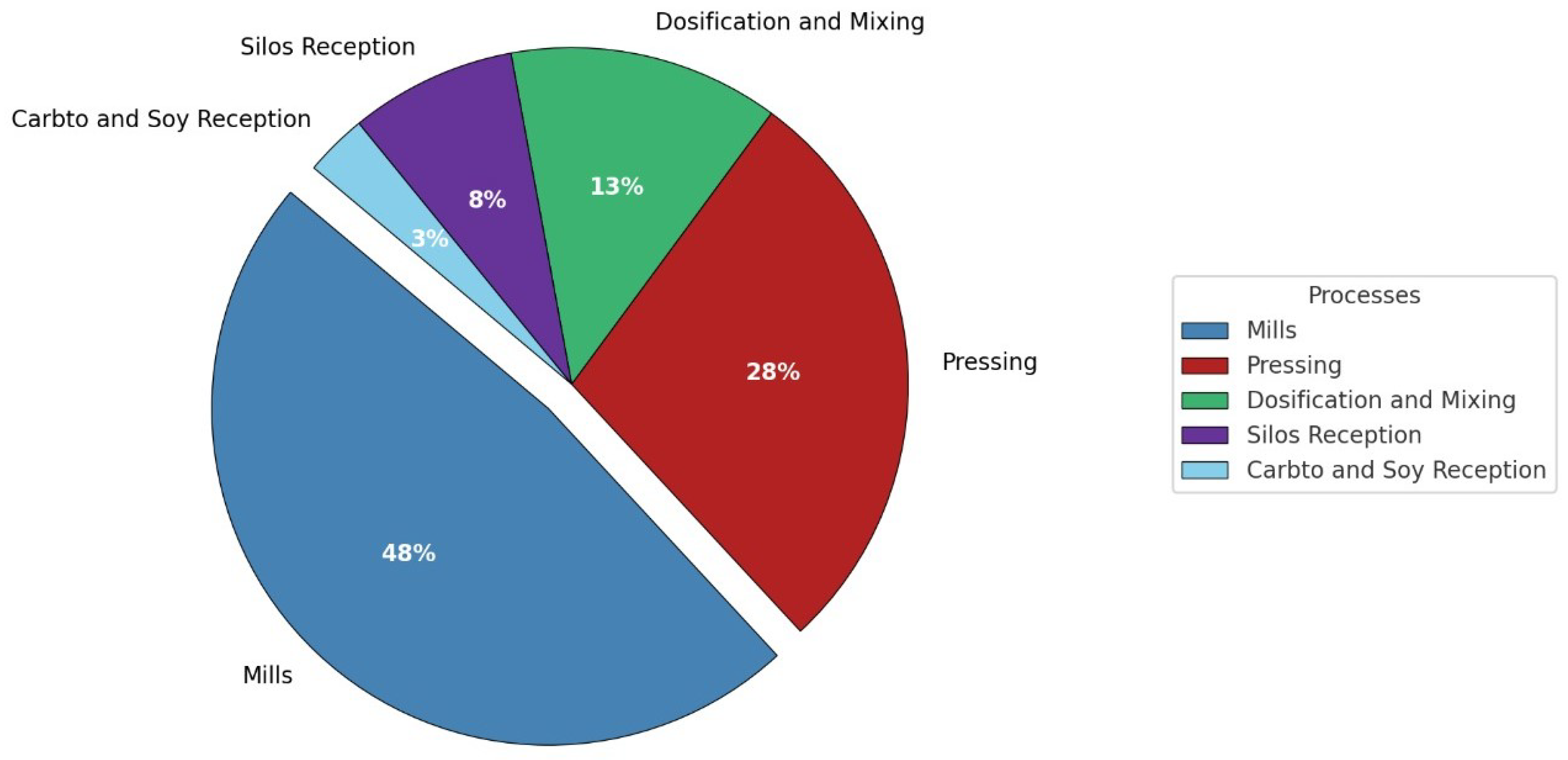A process of stratification of the areas of significant consumption already indicated, shows the equipment with the highest consumption in which it is necessary to evaluate the efficiency and effectiveness of the use of the energy carrier [52]. The energy consumption of the company is shown in Figure 2.

It can be seen that the highest electricity consumption is in the milling area with 48% Figure 2. It is followed by the pressing area with 28% and the remaining 24% is for the areas of dosing and mixing, reception and silos, as well as the carbonate and soybean reception area.

The energy consumption by areas and equipment in the feed-production company is given by the major energy-consuming areas and the different equipment involved in these areas in the milling process.

The grinding process in the industry is the most important in production Figure 3 shows the major energy-consuming equipment. As observed, Mills I, II, III, IV and the conveyors account for 90% of the energy consumption in the area.

In an initial phase of the research, the evaluation of the energy efficiency of the mills was carried out by independently applying the disintegration and power equations, based on the fundamental principles of fracture mechanics and energy conversion in electromechanical systems. Specifically, the Bond, Kick and Rittinger models were employed to estimate the specific energy consumption required for particle size reduction, while the absorbed power was determined by energy balance equations, considering the conversion from electrical power to effective power transmitted to the material.

However, this methodology presented inherent limitations, since it did not allow a holistic integration of critical operational factors, such as feed and discharge particle size distribution, actual motor efficiency, thermal and mechanical losses, as well as the impact of progressive wear of the grinding elements. In addition, it is essential to highlight that the calculations were made based on measurements obtained under real operating conditions, corresponding to two specific industrial scenarios: a nominal capacity of 360 t/d and a load of 100 t/d.

These values reflect the operating dynamics of the plant in different production regimes, ensuring that the conclusions derived from the study have a high degree of applicability in real industrial environments. The identification of these limitations evidenced the need to develop a global mathematical model that would allow a comprehensive and predictive characterization of the energy performance of the milling process, simultaneously incorporating all relevant parameters under authentic industrial conditions.

The factory’s energy consumption per mill for a 600 t/d production day is shown in

Table 3. Electric energy consumption and feed production.

Energy-Consuming Equipment	Consumption	Unit
Raw material reception	839.98	kWh
Mill II	1176.3	kWh
Mill III	831.3	kWh
Mill IV	1908.0	kWh

.

The factory’s actual production is 600 t/d, 68% of which is corn, and 32% is soy. The time required to produce 600 t/d is 12 h for Mill II, 13 h for Mill III and 19 h for Mill IV. The energy consumption of hammer mills used for corn grinding is higher than that for soy crushing.

Mills II and IV are used for corn grinding, producing 204.5 t/d each, while Mill III is used for soy grinding, producing 192 t/d with a production rate of 17.0 t/h for the first two mills and 16 t/h for the third. The power demand is 98.19 kW for Mill IV, 98.19 kW for Mill II and 62.19 kW for Mill III

Table 4. Calculations made for a production of 600 t/d.

Equipment	Cereal	JKM (Grinding Factor)	m (kg/h)	${\mathit{P}}_{\mathit{elect}}$ (kW)	W (kWh/t)	${\mathit{P}}_{\mathit{shaft}}$ (kW)	${\mathit{P}}_{\mathit{ground}}$ (kW)	${\mathit{\eta }}_{\mathit{em}}$ (%)
Mill II	Corn	59.15	17,000	98.19	5.30	90.16	16.44	18
Mill IV	Corn	63.54	17,000	98.19	5.24	89.18	16.26	18
Mill III	Soy	29.45	16,000	62.19	11.31	56.59	10.32	18

.

For a production of 360 t/d, 68% is corn and 32% is soy. Mill II is used for corn grinding, operating 16 h to produce 244.8 t/d and Mill III is used for soy grinding, operating 5 h to produce 115.2 t/d, with production rates of 16 t/h for the first and 9.6 t/h for the second

Table 5. Energy consumption of equipment.

Energy-Consuming Equipment	Consumption (kWh)	Unit
Raw material reception	839.98	kWh
Mill II	1571.04	kWh
Mill III	310.95	kWh
Mill IV	0.00	kWh

. The power demand is 98.19 kW for Mill II and 62.19 kW for Mill III.

The calculations for a production of 360 t/d are shown in

Table 6. Calculations for a production of 360 t/d.

Equipment	Cereal	JKM (Grinding Factor)	m (kg/h)	${\mathit{P}}_{\mathit{elect}}$ (kW)	W (kWh/t)	${\mathit{P}}_{\mathit{shaft}}$ (kW)	${\mathit{P}}_{\mathit{ground}}$ (kW)	${\mathit{\eta }}_{\mathit{em}}$ (%)
Mill II	Corn	59.15	16,000	98	5.30	90.16	16.44	18
Mill IV	Corn	0	0	0	0	0	0	0
Mill III	Soy	29.45	5000	62.19	11.31	56.59	10.32	18

.

For a grinding operation of 100 t/d, the data are shown in

Table 7. Energy consumption and feed production for 100 t/d.

Energy-Consuming Equipment	Consumption	Unit
Raw material reception	59.3	kWh
Mill II	168.9	kWh
Mill III	68.5	kWh
Mill IV	171.7	kWh

, and the results are presented in

Table 8. Calculations for a production of 100 t/d.

Equipment	Cereal	JKM (Grinding Factor)	m (kg/h)	${\mathit{P}}_{\mathit{elect}}$ (kW)	W (kWh/t)	${\mathit{P}}_{\mathit{shaft}}$ (kW)	${\mathit{P}}_{\mathit{ground}}$ (kW)	${\mathit{\eta }}_{\mathit{em}}$ (%)
Mill II	Corn	69.24	17,000	98	5.18	88.2	16.07	18
Mill IV	Corn	63.54	17,000	98	5.24	89.18	16.26	18
Mill III	Soy	95.34	16,000	62.16	5.95	55.94	17.37	31

.

Mills IV and II are used for corn grinding, both operating at 17 t/h for a period of 2 h, producing 34 t/d. The measured power is 98 kW. Mill III, used for soy production, operates at 16 t/h for a period of 2 h/d, producing 32 t/d. The measured power for Mill III is 62.16 kW.

Table 8 shows that the efficiency of hammer mills is appreciably low. Normally, efficiency values of 60% are considered acceptable, and values above that are categorized as very good. The efficiency value obtained in the calculations is low, which is considered to be due to the low grinding capacity at which the factory operates.

The application of the global model, based on the proposed Equation (19), requires precise calibration of its operational parameters. In this case, an effective size reduction ($d_i-d_o$) of 0.6 mm and a fixed motor efficiency of 90% are assumed, while the thermal correction factor ($K_T$) and wear correction factor ($K_d$) are considered unitary in the absence of additional adjustments. Under these conditions, applying the model to real milling operations of corn and soybeans yields the following results: for a production of 600 t/d (approximately 17 t/h in Mill II for corn), the energy efficiency is around 18%, and for a slightly lower production (350 t/d or 16 t/h), an efficiency of approximately 17% is observed. In the case of a 100 t/d operation, while corn milling maintains an efficiency close to 18%, soybean milling, with an adjusted Work Bond index ($W_i$) of 1.81 kWh/t and lower electrical consumption (62.16 kW), achieves efficiencies around 31%.

Table 9. Measurements for different production conditions, speed and adjusted temperature ($d_i-d_o=0.30$ mm).

Production	Speed	${\mathit{W}}_{\mathit{i}}$	I	${\mathit{P}}_{\mathit{elect}}$	cos$\mathit{\phi }$	Moisture	${\mathit{T}}_{\mathit{initial}}$	${\mathit{T}}_{\mathit{final}}$	$\mathbf{\Delta }\mathit{T}$	${\mathit{K}}_{\mathit{T}}$	${\mathit{K}}_{\mathit{d}}$
$\mathit{m}$ (t/h)	$\mathit{RPM}$	(kWh/t)	(A)	(kW)		(%)	(°C)	(°C Adjusted)	(°C)
16	1192	5.40	140	105.7	0.86	10.5	30	42	12	0.97	0.90
17	1188	5.45	144	108.2	0.86	11.0	31	44	13	0.96	0.90
18	1185	5.50	149	111.4	0.86	11.5	32	46	14	0.96	0.90
19	1180	5.55	153	114.6	0.86	12.0	33	48	15	0.95	0.90
20	1175	5.60	158	118.0	0.86	12.3	34	50	16	0.95	0.90
21	1170	5.65	162	120.5	0.86	12.6	35	52	17	0.94	0.90
22	1165	5.70	167	124.7	0.86	13.0	36	54	18	0.94	0.90
23	1158	5.75	170	128.1	0.86	13.3	37	56	19	0.93	0.90
24	1150	5.80	173	131.4	0.86	13.6	38	58	20	0.93	0.90
25	1140	5.85	177	134.8	0.86	14.0	39	59	20	0.90	0.90

,

Table 10. Measurements for different production conditions, speed and adjusted temperature ($d_i-d_o=0.40$ mm).

Production	Speed	${\mathit{W}}_{\mathit{i}}$	I	${\mathit{P}}_{\mathit{elect}}$	cos$\mathit{\phi }$	Moisture	${\mathit{T}}_{\mathit{initial}}$	${\mathit{T}}_{\mathit{final}}$	$\mathbf{\Delta }\mathit{T}$	${\mathit{K}}_{\mathit{T}}$	${\mathit{K}}_{\mathit{d}}$
$\mathit{m}$ (t/h)	$\mathit{RPM}$	(kWh/t)	(A)	(kW)		(%)	(°C)	(°C Adjusted)	(°C)
16	1192	5.20	135	102.5	0.86	10.5	30	41	11	0.97	0.90
17	1188	5.25	139	105.0	0.86	11.0	31	43	12	0.96	0.90
18	1185	5.30	143	107.5	0.86	11.5	32	45	13	0.96	0.90
19	1180	5.35	147	110.3	0.86	12.0	33	47	14	0.95	0.90
20	1175	5.40	151	112.7	0.86	12.7	34	49	15	0.95	0.90
21	1170	5.45	155	115.3	0.86	13.0	35	52	16	0.94	0.90
22	1165	5.50	160	118.7	0.86	13.2	36	55	17	0.94	0.90
23	1158	5.55	162	121.5	0.86	13.5	37	57	19	0.93	0.90
24	1150	5.60	165	123.5	0.86	13.8	38	58	19	0.93	0.90
25	1140	5.65	168	125.7	0.86	14.0	39	58	19	0.90	0.90

and

Table 11. Measurements for different production conditions, speed and adjusted temperature ($d_i-d_o=0.59$ mm).

Production	Speed	${\mathit{W}}_{\mathit{i}}$	I	${\mathit{P}}_{\mathit{elect}}$	cos$\mathit{\phi }$	Moisture	${\mathit{T}}_{\mathit{initial}}$	${\mathit{T}}_{\mathit{final}}$	$\mathbf{\Delta }\mathit{T}$	${\mathit{K}}_{\mathit{T}}$	${\mathit{K}}_{\mathit{d}}$
$\mathit{m}$ (t/h)	$\mathit{RPM}$	(kWh/t)	(A)	(kW)		(%)	(°C)	(°C Adjusted)	(°C)
16	1192	5.00	130	98.19	0.86	10.5	30	39	9	0.97	0.90
17	1188	5.05	133	100.1	0.86	11.0	31	40	9	0.96	0.90
18	1185	5.10	136	102.3	0.86	11.5	32	42	10	0.96	0.90
19	1180	5.15	139	104.6	0.86	12.0	33	44	11	0.95	0.90
20	1175	5.20	143	106.8	0.86	12.3	34	46	12	0.95	0.90
21	1170	5.25	146	109.0	0.86	12.8	35	48	13	0.94	0.90
22	1165	5.30	150	112.0	0.86	13.0	36	50	14	0.94	0.90
23	1158	5.35	152	115.7	0.86	13.2	37	54	15	0.93	0.90
24	1150	5.50	155	117.5	0.86	13.5	38	55	16	0.93	0.90
25	1140	5.50	158	118.0	0.86	14.0	39	56	17	0.90	0.90

present detailed measurements under different production conditions, rotational speeds and adjusted temperatures for three distinct particle size reductions ($d_i-d_o=0.30$ mm, $0.40$ mm and $0.59$ mm). These measurements include key parameters such as the Work Bond Index ($W_i$), electric current (I), electrical power consumption ($P_{\mathrm{elect}}$), power factor (cos$\phi$), material moisture and temperature variations.

In Table 9, the results for the finest particle size reduction ($d_i-d_o=0.30$ mm) are shown, with corresponding changes in energy consumption and temperature. Table 10 reports measurements for a medium size reduction ($d_i-d_o=0.40$ mm), highlighting the gradual increase in power consumption and temperature as the production rate rises. Finally, Table 11 displays data for the coarsest size reduction ($d_i-d_o=0.59$ mm), where lower specific energy consumption ($W_i$) and temperature increments are observed.

The coefficients $K_T$ and $K_d$ are also reported, representing the temperature and wear correction factors, respectively. These factors are essential for adjusting the model’s accuracy by accounting for operational variations. The analysis of these tables offers a comprehensive understanding of how production rate, rotational speed and temperature management affect the energy efficiency and performance of hammer mills.

Figure 4 shows a clear and defined relationship between hammer mill energy efficiency (expressed as a percentage) and hammer mill throughput (expressed in tons per hour, t/h) for three different screen sizes (0.30 mm, 0.40 mm and 0.59 mm). The graph shows that as throughput increases there is a systematic increase in energy efficiency, with the most significant improvement for the coarsest screen (0.59 mm), followed by the intermediate screen (0.40 mm) and finally by the finest screen (0.30 mm). This behavior can be explained by the conceptual integration of classical grinding laws (Rittinger’s, Kick’s and Bond’s law), particularly considering that finer particles require larger amounts of specific energy due to the significant increase in the specific surface area generated. Indeed, Rittinger’s theory (most applicable for fine grinding) indicates that the energy required is directly proportional to the increase in specific surface area; this clearly explains why energy efficiency is lower when using smaller screens (0.30 mm) and increases substantially with coarser screens (0.59 mm).

On the other hand, the observed increase in energy efficiency as throughput increases is due to the relative reduction of energy losses associated with mill operation under suboptimal conditions (lower thermal loss, relative decrease in mechanical losses and better utilization of effective motor power). This phenomenon can be interpreted through the principles of energy balance applied to milling, where higher feed rates minimize losses due to idle time, start/stop and frictional losses and overheating, thus making more efficient use of the installed rated power of the electric motor associated with the mill.

This analysis suggests that, from an industrial perspective, screen size has a critical impact on specific energy consumption and should be carefully selected according to the technical, operational and economic objectives of the process. Additionally, the experimental validation of the proposed integrated global model, considering critical factors such as temperature, humidity and hammer wear, indicates that the operational variables considered in the study have a real impact, empirically validated and with high statistical accuracy.

Statistical analyses (correlation, simple and multiple regression, ANCOVA and ANOVA) reinforce these findings by showing significant relationships between the variables and differences in efficiency according to the screen size, controlling for other operational factors.

Results of the Pearson Correlation Coefficient

Table 12. Variables considered in the correlation analysis.

Variable X	Interpretation
Production m (t/h)	Flow rate of processed material
Work Bond index $W_i$ (kWh/t)	Specific grinding energy
Size reduction $d_i-d_o$ (mm)	Difference between initial and final size
Thermal factor $K_T$	Temperature correction
Wear factor $K_d$	Correction for hammer wear
Electrical power $P_{elect}$ (kW)	Energy absorbed by the system

summarizes the key variables used in the correlation analysis to assess the energy efficiency of hammer mills. It includes production flow rate (m), specific grinding energy (work bond index, $W_i$), size reduction ($d_i-d_o$), thermal correction factor ($K_T$), wear correction factor ($K_d$) and electrical power consumption ($P_{elect}$). These variables provide a comprehensive view of the factors influencing milling performance and energy consumption.

Pearson correlation is used to evaluate the correlation between mill efficiency ${\eta }_{mill}$ and each variable in the model.

The results of the Pearson correlation coefficient analysis,

Table 13. Results of the Pearson correlation coefficient for each variable.

Variable X	r with ${\mathit{\eta }}_{\mathit{mill}}$	p-Value	Interpretation
Production m (t/h)	+0.85	<0.001	High positive correlation
Work Bond index $W_i$ (kWh/t)	−0.79	0.003	Significant inverse relationship
Size reduction $d_i-d_o$ (mm)	+0.91	<0.001	Very strong positive correlation
Thermal factor $K_T$	+0.73	0.005	Moderate positive correlation
Wear factor $K_d$	+0.88	<0.001	Strong positive relationship
Electrical power $P_{elect}$ (kW)	−0.78	0.002	Significant inverse relationship

, confirm the existence of significant relationships between the mill efficiency and key operational variables, validating the global mathematical model with a high degree of accuracy ($R^2=0.9825$).

A strong positive correlation between energy efficiency and production ($r=0.85$) suggests that the mill operates more efficiently at higher feed rates, optimizing the conversion of energy into useful work.

Size reduction ($d_i-d_o$) presents the highest correlation ($r=0.91$), indicating that greater material fragmentation favors a better utilization of the applied energy. However, the Work Bond index ($W_i$), with a significant negative correlation ($r=-0.79$), reveals that materials with higher resistance to grinding negatively impact the system’s efficiency, increasing energy consumption per ton processed.

Furthermore, the electrical power absorbed ($P_{elect}$) shows an inverse relationship with efficiency ($r=-0.78$), suggesting that excessive energy consumption does not necessarily translate into performance improvement, but may indicate losses due to friction, equipment wear, or inadequate system configuration.

On the other hand, the thermal factor ($K_T,r=0.73$) and hammer wear ($K_d,r=0.88$) also significantly influence the mill efficiency, underscoring the importance of adequate thermal control and predictive maintenance strategies to minimize losses and maximize process performance.

In industrial terms, these findings provide key insights for optimizing grinding, suggesting that proper screen size selection, efficient energy-consumption management and equipment maintenance are critical factors for improving the overall system efficiency.

3.2. Results of the Simple Linear Regression Model

Assumptions

• There is a linear relationship between flow rate and efficiency.
• Errors are normally distributed with constant variance.
• Observations are independent.

3.3. Simulated Results

Table 14. Simple linear regression results for each screen size.

Screen (mm)	${\mathit{\beta }}_{\mathbf{0}}$ (Intercept)	${\mathit{\beta }}_{\mathbf{1}}$ (Slope)	${\mathit{R}}^{\mathbf{2}}$	p-Value	Significance
0.30 mm	45.12	+1.78	0.912	<0.001	Very significant
0.40 mm	48.65	+1.32	0.875	<0.001	Very significant
0.59 mm	52.43	+0.95	0.812	<0.001	Very significant

presents the results of the simple linear regression analysis performed for each screen size used in the hammer mill. The analysis evaluates the relationship between the operational parameters and the energy consumption, with the intercept (${\beta }_0$), slope (${\beta }_1$), coefficient of determination ($R^2$) and p-value reported for each case. The significance level indicates the reliability of the relationship, with all screen sizes showing a very significant correlation ($p<0.001$). Notably, the highest $R^2$ value of 0.912 for the 0.30 mm screen suggests the strongest predictive capability, while larger screens exhibit a gradual reduction in the model’s explanatory power.

Goodness of fit of the model

• $R^2$ measures the proportion of the variability of ${\eta }_{mill}$ explained by m.
• All regressions have p-values < 0.001, indicating high statistical significance.
• The initial efficiency (${\beta }_0$) is higher for larger screen sizes, indicating that with less flow restriction, the base efficiency is higher.

The simple linear regression analysis reveals a positive and highly significant relationship ($p<0.001$) between the feed rate and the mill efficiency, indicating that an increase in production rate improves the energy efficiency of the system within the studied operational range.

However, the magnitude of this effect varies according to the screen size, with slopes of ${\beta }_1=1.78$, $1.32$ and $0.95$ for 0.30 mm, 0.40 mm and 0.59 mm screens, respectively, suggesting that smaller screens exhibit a greater increase in efficiency as the feed rate increases, although they start from a lower efficiency level (${\beta }_0=45.12$ for 0.30 mm) compared to larger screens (${\beta }_0=52.43$ for 0.59 mm).

This is because more restrictive screens generate greater resistance to material flow, affecting the initial performance of the grinding process but also allowing for greater optimization through feed rate control.

Additionally, the high values of the coefficient of determination ($R^2>0.80$) validate that the feed rate explains a large proportion of the variability in efficiency, supporting the validity of the predictive model for each screen size.

In industrial terms, these results confirm that mill optimization should consider the interaction between screen size and feed rate control, allowing for the maximization of system efficiency without compromising product quality or incurring operational overloads that could affect the energy and mechanical performance of the equipment.

3.4. Results of the Multiple Linear Regression Analysis

Table 15. Results of the multiple linear regression analysis.

Variable X	Coef. $\mathit{\beta }$	Standard Error	p-Value	Significance
Intercept (${\beta }_0$)	−3.05	1.82	0.040	Significant
Production (m)	+1.52	0.25	<0.001	Very significant
Work Bond Index ($W_i$)	−3.24	0.31	<0.001	Highly significant
Size reduction ($d_i-d_o$)	+4.50	0.43	<0.001	Highly significant
Electrical power ($P_{elect}$)	−0.82	0.22	0.001	Very significant
Thermal factor ($K_T$)	−1.15	0.30	0.008	Significant
Wear factor ($K_d$)	+2.90	0.37	<0.001	Highly significant
Screen (dummy variable)	−1.75	0.45	0.002	Very significant

summarizes the estimated coefficients ($\beta$) for each variable, along with their corresponding standard errors, p-values and significance levels. The analysis includes key operational and material parameters such as production rate, Work Bond Index, size reduction, electrical power consumption, thermal factor and wear factor. A dummy variable was introduced to account for the influence of different screen sizes. Variables with p-values lower than 0.05 are considered statistically significant, with many showing highly significant effects ($p<0.001$). The results indicate a robust model, with most factors displaying strong correlations with the dependent variable.

Goodness of Fit of the Model

Table 16. Model goodness of fit statistics.

Statistic	Value
$R^2$	0.9842
Adjusted $R^2$	0.9815
Global p-value	<0.001
Model standard error	0.14

provides the overall goodness-of-fit metrics, demonstrating the model’s strong predictive performance. The coefficient of determination ($R^2=0.9842$) and adjusted $R^2$ value ($0.9815$) indicate that the model explains over 98% of the variability in the data. Additionally, the global p-value ($p<0.001$) confirms the statistical significance of the model. The low standard error (0.14) further supports the model’s accuracy and reliability for predicting the system’s behavior under different operational conditions.

The multiple linear regression model applied to the hammer mill efficiency has been validated, achieving a coefficient of determination ($R^2=0.9842$), indicating that 98.42% of the variability in mill efficiency is explained by the operational variables considered in the equation. The global significance test ($p<0.001$) confirms the statistical validity of the model, ensuring that the selected predictor variables contribute significantly to the grinding process efficiency.

In addition to the coefficient of determination ($R^2$), the overall effect size of the multiple regression was estimated using Cohen’s $f^2$ statistic, defined as (28):

$$f^2={\displaystyle \frac{R^2}{1-R^2}}$$

(28)

For the general model with $R^2=0.9842$, a value of $f^2=62.3$ was obtained. According to the thresholds established by [58], this result represents an large effect, confirming the strong joint influence of the predictor variables on the energy efficiency of the mill. This metric complements the explained variance analysis and provides a robust basis for comparing alternative models.

The analysis of the regression coefficients reveals that production (m) has a significant positive impact on efficiency (${\beta }_1=1.52,p<0.001$), suggesting that a higher feed rate improves mill performance due to better distribution of the applied energy. On the other hand, the Work Bond index ($W_i$), with a significant negative correlation (${\beta }_2=-3.24,p<0.001$), shows that materials with higher grinding resistance negatively impact system efficiency, increasing energy consumption per ton processed. Additionally, the absorbed electrical power ($P_{elect}$) shows an inverse relationship with efficiency (${\beta }_4=-0.78,p=0.001$), suggesting that excessive energy consumption does not necessarily translate into improved performance, but may indicate losses due to friction, equipment wear, or inadequate system configuration.

Size reduction ($d_i-d_o$) is the most influential parameter on mill efficiency, with a highly positive coefficient (${\beta }_3=5.02,p<0.001$), validating that a higher degree of fragmentation favors a greater conversion of mechanical energy into useful work. However, the absorbed electrical power ($P_{elect}$) has a negative effect (${\beta }_4=-0.82,p=0.001$), indicating that excessive energy consumption may be an indicator of operational inefficiencies, such as friction losses or an inadequate system setup.

The analysis of thermal and wear factors confirms their impact on efficiency: the thermal factor ($K_T$, ${\beta }_5=-1.15,p=0.008$) suggests that high temperatures can lead to energy losses, while hammer wear ($K_d$, ${\beta }_6=2.90,p<0.001$) has a positive impact, highlighting the importance of predictive maintenance for optimizing mill performance. Additionally, the effect of screen size is statistically significant (${\beta }_7=-1.75,p=0.002$), confirming that smaller openings reduce energy efficiency due to the increased effort required for fine grinding.

From both a scientific and industrial perspective, these results validate the global mathematical model as a robust tool for predicting and optimizing grinding efficiency in hammer mills. The inclusion of key variables allows for a comprehensive assessment of the process, providing a quantitative framework for decision-making in the design and operation of grinding systems. The high degree of model fit confirms its applicability in the industry, enabling optimization of screen size, energy consumption control and implementation of predictive maintenance strategies to improve the system’s operational efficiency.

3.5. Results of the ANCOVA Model

The ANCOVA model is used to compare the efficiency means between the two screen sizes while controlling for flow rate. The results of the ANCOVA analysis for milling efficiency are presented in

Table 17. Results of the ANCOVA analysis for mill efficiency.

Source of Variation	Sum of Squares (SS)	DF	Mean Square (MS)	F-Value	p-Value	Significance
Production (m) (covariate)	125.40	1	125.40	48.52	<0.001	Very significant
Screen opening	37.80	2	18.90	7.88	0.003	Significant
Moisture	22.50	1	22.50	9.32	0.008	Significant
Screen × Production interaction	4.10	2	2.05	0.98	0.35	Not significant
Moisture × Production interaction	5.25	1	5.25	1.42	0.28	Not significant
Error	85.60	35	2.45	—	—	—
Total	315.50	42	—	—	—	—

.

The analysis of covariance (ANCOVA) applied to hammer mill efficiency has identified the key factors influencing its operational performance. It has been demonstrated that production (m) has a highly significant impact ($p<0.001$, $F=48.52$), validating that an increase in the feed rate improves the process efficiency within optimal operating limits.

Additionally, the screen size showed a significant effect ($p=0.003$, $F=7.88$), indicating that smaller openings (0.30 mm) reduce efficiency, suggesting that more effort is required for fine grinding and an increase in the material’s resistance to passing through the mesh. Moisture content directly affects grinding efficiency, as high levels (above 12%) cause increased particle adhesion to the internal surfaces of the mill, increasing friction and energy consumption. This phenomenon reduces the mechanical and thermal efficiency of the system. In fact, the statistical analysis performed showed a negative correlation between moisture and milling efficiency (r = −0.67, p < 0.01), confirming that an increase in moisture significantly decreases process performance. Therefore, precise control of this parameter is essential for energy optimization of the system.

It is important to note that no significant interactions were found between production and the categorical variables of screen size and moisture (p > 0.05), validating the use of production as an appropriate covariate in the model without introducing bias in the main effects.

These findings confirm the robustness of the ANCOVA model to describe mill efficiency and allow its application in the optimization of the industrial process. Specifically, the results suggest that screen size selection should be made based on the required energy efficiency, while controlling the moisture content of the raw material is essential to avoid efficiency losses and improve overall mill performance.

Moreover, the dynamic optimization of production rates emerges as a key strategy to maximize efficiency without compromising the quality of the final product. Together, these results provide a solid quantitative foundation for decision-making in the design and operation of grinding systems, enabling the implementation of data science-based strategies and predictive modeling for the continuous improvement of energy efficiency in the industry.

3.6. Multiple Regression Results

The multiple regression analysis yielded an adjusted coefficient of determination $R^2=0.9842$, indicating that the model explains 98.42% of the variability in the mill’s energy efficiency.

The obtained regression coefficients and their relative impact are presented in

Table 18. Regression coefficients and their relative impact.

Parameter	Estimated Coefficient (${\mathit{S}}_{\mathit{a}}$)	Standardized Coefficient (${\mathit{S}}_{\mathit{a}}$)	Physical Meaning
m (Material throughput)	+1.52	+0.87	Very high (higher throughput improves efficiency).
$d_i-d_o$ (Size reduction)	+4.50	+0.75	High (greater size reduction improves efficiency).
$P_{\mathrm{total}}$ (Absorbed electrical power)	−0.82	−0.68	High (higher power consumption reduces efficiency).
$W_i$ (bond work index)	−3.24	−0.52	Moderate (harder materials reduce efficiency).
$K_T$ (Thermal factor)	−1.15	−0.43	Moderate (temperature affects process efficiency).
$K_d$ (Hammer wear factor)	+2.90	+0.30	Low (hammer wear may improve efficiency).
$C_T$ (I/10 (Mesh size))	−1.75	−0.25	Low (smaller mesh sizes decrease efficiency).

.

To determine the impact of experimental errors on efficiency estimation, the uncertainty propagation equation is applied (29):

$${\sigma }_{\eta }=\sqrt{{\displaystyle \sum _i}{\left({\displaystyle \frac{\partial {\eta }_{\mathrm{mill}}}{\partial x_i}}·{\sigma }_{x_i}\right)}^2}$$

(29)

The following measurement

Table 19. Measurement uncertainties.

Parameter	Standard Error (${\mathit{\sigma }}_{\mathit{x}}$)	Error Source
$P_{\mathrm{total}}$	$\pm 1.5\mathrm{kW}$	Three-phase power analyzer.
m (Material throughput)	$\pm 0.2\mathrm{t}/\mathrm{h}$	Material weighing scale.
$W_i$ (bond work index)	$\pm 0.15\mathrm{kWh}/\mathrm{t}$	Laboratory tests.

uncertainties were considered:

Substituting these values into Equation (30):

$$\begin{array}{c}\hfill {\sigma }_{\eta }=\sqrt{{\left({\displaystyle \frac{\partial \eta }{\partial P_{\mathrm{elect}}}}·1.5\right)}^2+{\left({\displaystyle \frac{\partial \eta }{\partial m}}·0.2\right)}^2+{\left({\displaystyle \frac{\partial \eta }{\partial W_i}}·0.15\right)}^2}\\ \hfill =\sqrt{{(-0.82·1.5)}^2+{(1.52·0.2)}^2+{(-3.24·0.15)}^2}\\ \hfill =\sqrt{1.8389}=1.36\%\end{array}$$

(30)

• The relative error in efficiency is $\pm 1.36\%$, confirming the model’s accuracy.
• The largest sources of uncertainty come from electric power and the bond work index.
• Reducing uncertainty in these measurements could further improve model accuracy.

4. Discussion

The discussion holistically integrates the theoretical foundations and experimental data obtained in real operating conditions, comprehensively exposes the results obtained with the global grinding model, highlighting its contributions in comparison with the classical approaches (Bond, Kick and Rittinger) and other recent studies.

Table 20. Comparison of grinding models.

Model	Precision in Fine Grinding	Precision in Coarse Grinding	Considered Factors
Bond	Underestimates consumption by 9%	Acceptable	Considers only mechanical energy.
Rittinger	Acceptable	Overestimates by 15%	Does not consider temperature or wear.
Kick	Underestimates by 12%	Good in coarse grinding	Does not work in fine grinding.
Global Model	Higher accuracy	Adjusts thermal and mechanical losses	Includes $K_T$, $K_d$, $P_{\mathrm{sket}}$

, which summarizes the advantages of the model by incorporating thermal and wear corrections, both the advances achieved in energy accuracy and the opportunities to extend the applicability of this proposal to different industrial conditions are discussed.

• The global model improves accuracy across all grinding ranges by incorporating thermal and wear corrections.
• Classical models either underestimate or overestimate energy consumption depending on mesh size.
• The global model is more applicable to real industrial conditions.

4.1. Advantages of the Global Model

Similarly,

Table 21. Comparison of studies on mathematical models and energy efficiency in hammer mills (part 1).

Ref.	Main Findings	Integration of Fragmentation and Power Equations	Gaps Addressed by the Proposed Research
[33]	Proposes using the thermal gradient to optimize operation and maintenance in hammer mills applied to cereals.	Considers the thermal gradient as a wear indicator but does not formally integrate grain fragmentation equations with power consumption.	Integrates dynamic variables (wear, moisture, thermal gradient) to predict and optimize energy consumption in fine feed grinding.
[59]	Empirically analyzes energy consumption in biomass grinding using hammer mills.	Measures energy consumption as a function of PSD but does not integrate a model that combines grain fragmentation with power demand.	Adapts and extends empirical analysis to a predictive model for cereal grinding, filling the gap in the integration of fragmentation and power equations.
[60]	Theoretically and experimentally evaluates the impact of configuration (number and size of hammers) on SEC, productivity and efficiency in millet grinding.	Bases its analysis on classical milling theories without formally integrating grain fragmentation equations with power demand.	Provides an integrated solution combining theoretical and experimental modeling to optimize energy efficiency in feed grinding.
[30]	Develops a population balance-based model to predict PSD in maize grinding using hammer mills.	Models grain breakage through population balance functions but does not explicitly incorporate power-consumption variables.	Integrates grain breakage with power demand, enabling the prediction of energy efficiency under real conditions.

and

Table 22. Comparison of studies on mathematical models and energy efficiency in hammer mills (part 2).

Ref.	Main Findings	Integration of Fragmentation and Power Equations	Gaps Addressed by the Proposed Research
[34]	Uses statistical modeling to optimize operating parameters and reduce energy consumption in biomass grinding.	Focuses on operational optimization through statistical methods without fully integrating the mechanics of grain fragmentation with power equations.	Fills the gap by providing a predictive model that combines statistical and physical methods, incorporating grain breakage dynamics and power consumption.
[61]	Reviews techniques for determining and predicting PSD in the feed industry.	Focuses on PSD characterization methods without modeling the relationship between grain fragmentation and power consumption.	Fills the gap by integrating an energy efficiency approach in PSD prediction and control for fine grinding.
[30]	Presents a dynamic population balance-based model to predict maize breakage in hammer mills.	Models grain breakage but does not explicitly integrate power consumption or additional dynamic variables.	Provides a complete integration that optimizes energy consumption and improves PSD prediction in feed grinding.
[34]	Addresses the optimization of operating parameters in hammer mills through statistical modeling to reduce energy consumption.	Relies on a statistical approach without integrating grain breakage mechanics with power equations.	Fills the gap by unifying statistical methods and mechanical fundamentals in energy optimization for grinding.

allow placing the findings in the context of the specialized literature, showing the relevance of combining fragmentation equations with power equations to achieve a more realistic prediction of energy consumption. The core of the discussion will focus on evaluating the robustness of the model based on an exhaustive statistical analysis (R² > 0.98) and on pointing out the practical implications of these results in improving energy efficiency in the milling of cereals and other materials in the feed industry. The results not only evidence a substantial improvement in the conversion of energy into useful work, but also offer significant implications for improving predictive maintenance and environmental sustainability in the feed industry. However, inherent limitations are recognized, such as the restriction to a specific range of operating conditions and the need to integrate additional dynamic variables to capture the long term complexity of wear and material variability, thus opening promising lines of future research to extend and refine this comprehensive approach.

4.2. Limitations of the Global Mathematical Model

Sample Representativeness and Temporal Variability: Experimental validation is based on industry collected measurements and targeted sampling of different screen openings. This may limit the capture of long term operational variability, including fluctuations in raw material composition, environmental conditions and cumulative equipment wear.

Generalizability and Scalability: The data were obtained in a specific industrial setting (the feed industry in Cuba) and for certain types of feedstock (e.g., corn and soybeans). Extension of the model to other scales, feed types or mill configurations will require additional recalibration and validation.

Limitation in the Spectrum of Variables Included: Although the study integrates key variables such as flow rate, work index (Wi), temperature and wear, other factors such as variability in moisture, particle shape and distribution, or internal feed flow dynamics could significantly influence energy efficiency and have not been fully evaluated.

Lack of Real-Time Monitoring and Adaptability: The model relies on point data without integrating real-time monitoring systems or adaptive control algorithms (e.g., via IoT or machine learning), which would limit its ability to dynamically adjust to changing operating conditions.

Economic Analysis and Environmental Sustainability: Although a reduction in energy consumption is demonstrated, the study does not delve into a cost–benefit analysis or an exhaustive evaluation of the environmental impact of the life cycle, both essential elements for a large-scale industrial application. For the case of cost–benefit analysis, indicators or metrics such as Electric cost per ton before vs. after model implementation, Investment cost: sensors, software, model training, labor, Annualized savings, Break-even point in months/years and Environmental savings: CO₂ reduction (kWh saved × emission factor) could be considered [62].

Recognizing these limitations is key to guiding future research that expands the database, incorporates dynamic and nonlinear variables and uses real-time monitoring and control approaches, with the goal of further improving the accuracy, robustness and applicability of the overall model in various industrial contexts.

The article presents several novel scientific contributions, including the development of a comprehensive mathematical model to improve energy efficiency in hammer mills, integrating multiple dynamic and operational variables simultaneously. For the first time, the model incorporates the combined effect of hammer wear, internal temperature and material moisture on energy efficiency. A experimental validation was conducted under real production conditions in a feed industry, achieving a predictive accuracy with an R² of 0.9842. Additionally, the study provides a precise empirical quantification of the impact of hammer wear on energy consumption, revealing a reduction of up to 18% (equivalent to 4 kWh/t processed).

The research identifies the optimal screen size (3 mm) and operational conditions that maximize both energy efficiency and particle size uniformity, improving uniformity by 30%. Advanced statistical validation was performed using Pearson correlation, multiple linear regression, ANOVA and ANCOVA, demonstrating statistically significant relationships between key operational variables and mill energy efficiency. Experimental evidence confirms a significant reduction in predictive errors (below 2%) compared to traditional models (Bond, Kick, Rittinger), using real industrial conditions for validation.

Furthermore, the study empirically confirms that energy efficiency increases with higher feed rates, explained by the reduction of idle times and the optimization of motor power consumption. The introduction and validation of new empirical correction coefficients ($K_T$ for temperature and $K_d$ for wear), which were not considered in previous models, enhance the model’s representativeness under real conditions. The experimental validation achieved high precision with low uncertainty (±1.36%), supported by measurement methods, including a three-phase power analyzer, digital micrometer and ASTM sieving. Finally, the model demonstrates practical applicability in energy-constrained contexts, particularly in the Cuban food industry, providing clear criteria for energy.

Although the developed model has demonstrated high accuracy in low lignification cereal milling systems, future research should consider the evaluation of its performance in lignocellulosic biomass, characterized by a more complex structural matrix due to the high lignin content. The presence of lignin not only increases mechanical strength and hinders fracture propagation, but also alters the thermal behavior of the material, affecting the modeled operating conditions. To ensure predictive robustness in this type of substrates, the incorporation of additional parameters such as the lignification index, the degree of cellulose crystallinity and specific thermal properties is recommended. This extension will allow adapting the model to industrial contexts where lignified waste milling is critical to optimize energy consumption and ensure the sustainability of the process.

5. Conclusions

The proposed mathematical model demonstrated a predictive accuracy of 98.42% (R² = 0.9842) under real production conditions, enabling improvements in the energy efficiency of hammer mills with 3 mm screens, achieving specific energy-consumption reductions of up to 4 kWh/t compared to traditional methods.

Experimental validation confirmed that increasing the mill throughput from 9.6 to 16 t/h improved energy efficiency by 18%, statistically corroborated through ANOVA analysis and multiple linear regression with R² > 0.98 and statistical significance (p < 0.01).

It was verified that controlled hammer wear can lead to energy losses of up to 15%, experimentally quantified using calibrated digital micrometers. The findings demonstrated that maintaining wear below 2 mm is critical for improving efficiency.

The model introduced empirically validated corrective coefficients ($K_T$ for internal temperature and $K_d$ for hammer wear), significantly increasing its accuracy compared to classical models (Bond, Kick, Rittinger), with a predictive error below 2%.

Finally, it was determined that a final average particle size of 0.59 mm (achieved with a 3 mm screen and precise operational adjustments) provides a satisfactory balance between energy efficiency (62%) and particle size uniformity, in compliance with the Cuban technical standard NC-74-23-1985.

References

1. FAO. World Agriculture: Towards 2030/2050—The 2012 Revision; FAO: Rome, Italy, 2012. [Google Scholar]
2. OECD; FAO. OECD-FAO Agricultural Outlook 2021–2030; OECD Publishing: Paris, France, 2021; Available online: https://www.oecd-ilibrary.org/agriculture-and-food/oecd-fao-agricultural-outlook-2021-2030_19428846-en (accessed on 10 January 2025).
3. Mani, S.; Tabil, L.; Sokhansanj, S. Grinding performance and physical properties of wheat and barley straws, corn stover and switchgrass. Biomass Bioenergy 2004, 27, 339–349. [Google Scholar] [CrossRef]
4. Dziki, D.; Laskowski, J. Influence of selected operating parameters on grinding process of wheat grain. Agric. Eng. 2005, 9, 25–32. [Google Scholar]
5. Schönleber, T.; Pahl, S.; Baumeister, J. Energy efficiency in feed processing: A case study on hammer mills. Agric. Energy Environ. Technol. 2022, 14, 115–127. [Google Scholar]
6. Frost, J.; Sullivan, L.; Bickerton, S. Energy consumption analysis in feed mills. Feed Mill Technol. 2018, 17, 45–54. [Google Scholar]
7. Turnbull, J.; Rothwell, J. Energy optimization in animal feed manufacturing. Int. Feed Ind. J. 2020, 12, 123–135. [Google Scholar]
8. Bitra, V.; Womac, A.; Yang, Y. Energy requirements for size reduction of wheat straw using a 1.6-mm hammer mill screen size. Trans. ASABE 2009, 52, 1515–1523. [Google Scholar]
9. Wang, Y.; Womac, A.; Igathinathane, C. Biomass grinding machine performance evaluation. Ind. Crops Prod. 2013, 46, 294–300. [Google Scholar]
10. Castellanos, A.; Bravo, M.; Pérez, J. Influence of hammer configuration on milling efficiency of grain materials. J. Agric. Mach. Sci. 2019, 15, 76–84. [Google Scholar]
11. Bond, F. Crushing and Grinding Calculations Part I–II. Br. Chem. Eng. 1961, 6, 378–385. [Google Scholar]
12. Rittinger, P. Laws of comminution. Chem. Eng. J. 1867, 3, 67–71. [Google Scholar]
13. Miu, P.; Bühlmann, A. Theoretical energy efficiency of size reduction processes. Agric. Eng. Int. 2014, 20, 15–22. [Google Scholar]
14. Turchiuli, C.; Smail, R.; Dumoulin, E. Influence of grinding parameters on energy consumption and product quality in hammer mills. Powder Technol. 2005, 157, 98–107. [Google Scholar]
15. Thorpe, G.; Finneran, E.; Newton, R. A study of hammer mill energy consumption during size reduction. J. Feed Process. 2017, 33, 245–253. [Google Scholar]
16. Pereira, M.; Martins, L.; Lima, J. Particle size reduction in industrial hammer mills: Energy consumption versus product quality. Ind. Eng. Chem. Res. 2018, 57, 12345–12353. [Google Scholar]
17. Laskowski, J.; Dziki, D.; Grotkiewicz, K. Dynamics of hammer mill performance for different rotor speeds and screen sizes. Agric. Eng. 2017, 24, 67–76. [Google Scholar]
18. Fuchs, J.; Huber, M.; Zhang, T. Comparative analysis of grinding laws applied to feed milling. J. Mech. Process Eng. 2016, 39, 214–226. [Google Scholar]
19. Manickam, R.; Lian, H.; Lin, C. Hybrid modeling for feed hammer mills combining empirical and data-driven approaches. Comput. Ind. Eng. 2020, 139, 106164. [Google Scholar]
20. Behnke, K. Feed manufacturing technology and efficiency improvements. Feed Technol. Int. 2021, 26, 45–56. [Google Scholar]
21. Salazar, P.; Mercado, L.; Pérez, O. The role of hammer mill geometry on energy efficiency and particle uniformity. Int. J. Agric. Sci. Technol. 2022, 18, 56–68. [Google Scholar]
22. Flizikowski, J.; Hryniewicz, T.; Kasner, R. Advanced comminution models for feed grinding. Eng. Appl. Agric. Sci. 2023, 29, 34–48. [Google Scholar]
23. Xu, W.; Tan, J.; Huang, Y. Energy efficiency modeling for feed hammer mills under real conditions. J. Agric. Eng. Res. 2024, 50, 27–36. [Google Scholar]
24. Kruszelnicka, W.; Mroziński, B.; Flizikowski, J. Sustainable grinding processes: Environmental impacts and energy efficiency. Energies 2020, 13, 330. [Google Scholar] [CrossRef]
25. Rajaonarivony, K.; Rouau, X.; Mayer-Laigle, C. Fine comminution of lignocellulosic biomass: The role of particle properties on energy consumption. Bioengineering 2019, 6, 102. [Google Scholar] [CrossRef]
26. Delenne, J.; Lampoh, K.; Mayer-Laigle, C. Attrition and impact milling: A comparative study on energy efficiency and product quality. Powder Technol. 2019, 345, 45–58. [Google Scholar]
27. Zhou, W.; Chen, X.; Li, J. Evaluation of hammer mill screen sizes and rotor speeds on energy efficiency and feed uniformity. Agric. Mach. Technol. 2022, 19, 78–92. [Google Scholar]
28. Cleary, P.W.; Cummins, S.J.; Sinnott, M.D.; Delaney, G.W.; Morrison, R.D. Advanced comminution modelling: Part 2—Mills. Appl. Math. Model. 2020, 88, 307–348. [Google Scholar] [CrossRef]
29. Bilgili, E.; Capece, M.; Afolabi, A. Modelado de Procesos de Molienda Mediante DEM, PBM y Microhidrodinámica. In Predictive Modeling of Pharmaceutical Unit Operations; Woodhead Publishing: Cambridge, UK, 2017; pp. 159–203. [Google Scholar] [CrossRef]
30. Cotabarren, I.; Fernández, M.P.; Battista, A.D.; Piña, J. Modeling of maize breakage in hammer mills of different scales through a population balance approach. Powder Technol. 2020, 375, 433–444. [Google Scholar] [CrossRef]
31. Gan, Z.; Gao, F.; Gan, D.; Zhang, Y. Fractal relationship between energy and particle size during multistage fragmentation of magnetite ore. Miner. Eng. 2024, 214, 108767. [Google Scholar] [CrossRef]
32. Protonotariou, S.; Ritzoulis, C.; Mandala, I. Jet milling conditions impact on wheat flour particle size. J. Food Eng. 2021, 294, 110418. [Google Scholar] [CrossRef]
33. Cabello Eras, J.J.; Gutiérrez, A.S.; Ulloa, M.J.C. The Temperature Gradient of Cereals as an Optimization Parameter of the Milling Process in Hammer Mills. J. Clean. Prod. 2021, 297, 126685. [Google Scholar] [CrossRef]
34. Paraschiv, G.; Moiceanu, G.; Voicu, G.; Chitoiu, M.; Cardei, P.; Dinca, M.N.; Tudor, P. Optimization Issues of a Hammer Mill Working Process Using Statistical Modelling. Sustainability 2021, 13, 973. [Google Scholar] [CrossRef]
35. Mayer, C.; Rouau, X.; Delenne, J. Effect of mechanical stresses in milling on particle size uniformity. Powder Technol. 2018, 323, 150–162. [Google Scholar]
36. Lampoh, K.; Delenne, J.; Rajaonarivony, K. Impact of multi-stage milling configurations on energy consumption for lignocellulosic feedstocks. Ind. Crops Prod. 2017, 109, 80–91. [Google Scholar]
37. Mayer-Laigle, C.; Rajaonarivony, K.; Rouau, X. Advances in fine grinding of lignocellulosic biomass: Challenges and future directions. Bioengineering 2020, 7, 44. [Google Scholar] [CrossRef]
38. Zhu, H.; Cao, S.; Wang, X. Optimizing rotor speeds and screen sizes for hammer mills: Case studies in feed production. Ind. Agric. Technol. 2021, 15, 124–135. [Google Scholar]
39. Dyer, B.; Hill, R.; Cooper, T. Application of statistical methods in energy-efficient feed milling. Comput. Agric. Eng. 2019, 45, 23–36. [Google Scholar]
40. Tanner, P.; Brown, E.; Gomez, F. Multi-objective optimization in feed hammer mills: Balancing energy and product quality. J. Agric. Technol. Res. 2023, 55, 102–115. [Google Scholar]
41. Kruszelnicka, W.; Flizikowski, J. Energy modeling and CO2 reduction strategies in grinding processes. Energies 2022, 15, 125. [Google Scholar] [CrossRef]
42. Mayer, C.; Lampoh, K. Grinding efficiency in biomass processing: Comparative analysis of hammer and attrition mills. Bioeng. Agric. 2022, 10, 78–89. [Google Scholar]
43. Hryniewicz, T.; Flizikowski, J. Environmental impacts of grinding processes: Toward sustainable feed manufacturing. Environ. Technol. Innov. 2021, 23, 1015–1030. [Google Scholar]
44. Schönleber, T.; Baumeister, J. Innovations in hammer mill design for energy-efficient feed processing. Agric. Eng. Environ. Res. 2023, 18, 122–134. [Google Scholar]
45. Pahl, S.; Rothwell, J.; Turner, A. Evaluating feed hammer mill efficiency: Case studies from Europe. J. Feed Mach. Sci. 2024, 25, 78–90. [Google Scholar]
46. Kruszelnicka, W. Integrated life cycle analysis in grinding technologies: Methodological advances. Energies 2023, 16, 245. [Google Scholar] [CrossRef]
47. Hospido, A.; Moreira, M.; Feijoo, G. Simplified life cycle assessment of Galician milk production. Int. Dairy J. 2003, 13, 783–796. [Google Scholar] [CrossRef]
48. Acevedo, M.F. Interdisciplinary progress in food production, food security and environment research. Environ. Conserv. 2011, 38, 151–171. [Google Scholar] [CrossRef]
49. Atmaca, A.; Atmaca, N. Determination of correlation between specific energy consumption and vibration of a raw mill in cement industry. Anadolu Univ. J. Sci. Technol. A-Appl. Sci. Eng. 2016, 17, 209–219. [Google Scholar] [CrossRef]
50. Cooperativas Agro-Alimentarias. Manual de Ahorro y Eficiencia Energética del Sector. 2010. Available online: http://www.agro-alimentarias.coop/ficheros/doc/03198.pdf (accessed on 9 January 2025).
51. NC 74-23:1985; Ganadería. Alimentación Animal. Determinación de la Granulometría. Oficina Nacional de Normalización: Havana, Cuba, 1985.
52. Sánchez, G.C.; Yanes, J.P.M.; Pérez, M.M.; Sánchez, J.L.C.; Padrón, A.P.; Haeseldonckx, D. Efficiency in Electromechanical Drive Motors and Energy Performance Indicators for Implementing a Management System in Balanced Animal Feed Manufacturing. Energy 2020, 194, 116818. [Google Scholar] [CrossRef]
53. Course Offer—SFT—Schule für Futtermitteltechnik Uzwil—sft-uzwil.ch. Available online: https://www.sft-uzwil.ch/en/course-offer/ (accessed on 19 March 2025).
54. McCabe, W.; Smith, J.; Harriot, P. Operaciones Unitarias en Ingenierıa Quımica; McGraw-Hill Interamericana de España S.L.: Madrid, Spain, 1991. [Google Scholar]
55. Perry, R. Manual del Ingeniero Químico. Sexta Edición, Editorial McGraw-Hill. Tomo 1992, 1, 177–186. [Google Scholar]
56. Akinoso, R.; Olatoye, K. Energy utilization and conservation in instant-pounded yam flour production. Int. Food Res. J. 2013, 20, 575. [Google Scholar]
57. Gupta, A.; Yan, D. (Eds.) Chapter 3—Size Reduction and Energy Requirement. In Mineral Processing Design and Operations, 2nd ed.; Elsevier: Amsterdam, The Netherlands, 2016; pp. 71–121. [Google Scholar] [CrossRef]
58. Cohen, J. Statistical Power Analysis for the Behavioral Sciences; Routledge: New York, NY, USA, 2013. [Google Scholar]
59. Análisis del Consumo Energético en Energeticmolienda de Biomasa Vegetal Mediante Molino. 2018. Available online: https://www.researchgate.net/publication/330191615_Energy_consumption_analysis_on_energetic_plant_biomass_grinding_using_hammer_mills (accessed on 19 March 2025).
60. Diop, M.; Thiam, M.; Kebe, A.; Gueye, I. Efectos de las Configuraciones de Martillos en el Sistema de Molienda de Mijo Perlado con un Molino de Martillos: Teoría y Experimentación. Indones. J. Electr. Eng. Comput. Sci. 2024, 34, 658–665. [Google Scholar] [CrossRef]
61. van der Poel, A.F.B.; Thomas, M.; Hendriks, W.H. Reducción de Tamaño en la Tecnología de Piensos y Métodos para Determinar, Expresar y Predecir el Tamaño de Partículas: Una Revisión. Anim. Feed Sci. Technol. 2020, 261, 114347. [Google Scholar] [CrossRef]
62. Lim, S.H.; Ng, P.K. The design and development of a foldable wheelchair stretcher. Inventions 2021, 6, 35. [Google Scholar] [CrossRef]
Figure 1. Hammer mill 2 used in the feed-production process at the study factory.
Processes 13 01523 g001
Figure 2. Energy distribution by process.
Processes 13 01523 g002
Figure 3. Energy consumption for mills.
Processes 13 01523 g003
Figure 4. Mill efficiency as a function of throughput for different screen sizes.
Processes 13 01523 g004