Incipient Fault Detection Based on Feature Adaptive Ensemble Net

Abstract

With the increasing complexity of modern industrial processes, fault occurrences may lead to catastrophic consequences, making incipient fault detection crucial for industrial safety. This critical task confronts a key challenge: insufficient cross-domain generalization capacity. To overcome this challenge, a feature adaptive ensemble net (FAENet) is proposed by integrating transfer learning with ensemble learning. The framework comprises a feature adaptive extractor (FAE) utilizing convolutional neural networks (CNNs) with maximum mean discrepancy (MMD) for domain-invariant feature extraction, combined with an information entropy gain-based feature screening to filter out redundant and detrimental features. In addition, the famous benchmark Tennessee Eastman process (TEP) and Case Western Reserve University (CWRU) bearing datasets are adopted to demonstrate the performance of the proposed method. For incipient difficult faults 3, 5, 9, 15, 16, and 21 in the TEP, FAENet achieves 99.43% for average fault detection rates (FDRs), exceeding traditional methods of cross-domain fault detection (TCA, JDA, DANN, DTL) by more than 60%. For CWRU’s incipient bearing faults, FAENet achieves 99.4% for FDR, demonstrating significant superiority. This research holds significant practical implications for enhancing the safety and efficiency of industrial systems. It establishes a reliable framework for intelligent fault detection systems across diverse industrial environments, enabling early detection of potential faults to minimize operational risks.

1. Introduction

Fault detection constitutes a fundamental method in modern engineering practice, with critical applications spanning industrial manufacturing, aerospace systems, and energy production sectors. This systematic approach enables continuous evaluation of equipment operational status through comprehensive monitoring protocols, facilitates early identification of potential abnormalities, and initiates preventive actions to avert critical failures and safety-related emergencies. The implementation of such detection frameworks significantly enhances operational safety parameters, improves system reliability metrics, and optimizes cost efficiency in complex industrial environments [1]. Over recent decades, substantial research efforts have been devoted to developing sophisticated data-driven methodologies for this purpose. Principal component analysis (PCA) projects the original data into principal component and residual subspaces and monitors variations in these subspaces [2]. Partial least squares (PLS) focuses on establishing the relationship between process and quality variables by extracting latent variables that maximize the covariance between them [3]. Considering the dynamics and nonlinearity in data, various variants of PCA and PLS have been developed, including dynamic PCA (DPCA) [4], kernel PCA [5], dynamic PLS [6], and kernel PLS [7].

In recent years, deep learning (DL) has emerged as a prominent technique for fault detection, owing to its powerful capabilities for automatic feature extraction [8]. Among various deep learning frameworks, CNNs have been widely applied in image-based fault detection tasks due to their ability to capture spatial hierarchical features [9]. Recurrent neural networks, especially long short-term memory networks, have demonstrated outstanding performance in time-series fault detection due to their capability to capture temporal dependencies within sequences [10]. Autoencoders are widely used in anomaly detection by learning the reconstruction of normal operating states, identifying deviations, and marking them as potential faults [11]. Deep belief networks have been widely researched due to their ability to learn hierarchical representations of data [12]. These deep learning methods have shown significantly superior performance compared to traditional approaches, particularly when dealing with complex nonlinear relationships in industrial systems.

However, traditional deep learning methods generally assume that the training and testing datasets follow the same distribution [13]. Furthermore, for the problem of fault detection, fault data in industrial environments are often scarce and costly to obtain, limiting the applicability of these methods in real-world scenarios [14]. To tackle the problem of data scarcity and distributional mismatch in fault detection, transfer learning (TL) has emerged as a promising solution. By transferring knowledge from a source to a target domain, TL reduces reliance on labeled data and enhances model generalization. It leverages experience gained from source tasks to improve learning for target tasks. Additionally, it boosts learning efficiency by utilizing existing models or features, thus lowering the computational cost of training from scratch. Transfer learning shows significant potential in incipient fault detection across varying conditions, devices, and environments, making it increasingly vital for intelligent fault detection systems [15].

TL has been effectively utilized in various fields, particularly in fault detection through methods such as parameter and feature transfer, along with domain adaptation [16]. Parameter transfer focuses on fine-tuning model parameters using target domain data. Shao et al. [17] applied pre-trained models for machine fault detection by converting sensor data into time–frequency images via wavelet transform and extracting low-level features with pre-trained networks. Zhang et al. [18] introduced a TL-based method that utilizes neural networks to learn from large-scale source data and adjust network parameters accordingly. Feature-based transfer learning aims to establish a function that maps features between the source and target domains. Wen et al. [19] developed a deep transfer learning approach based on a sparse autoencoder to mitigate performance degradation in traditional fault detection when training and testing data distributions differ. Wang et al. [20] proposed probabilistic transfer FA, which employs factor analysis to facilitate autonomous fault detection across varying operational conditions by identifying cross-domain feature spaces. Domain adaptation is an essential aspect of transfer learning, focusing on knowledge transfer from the source domain to the target domain by exploring domain-invariant features that address distributional divergences [21]. Lu et al. [22] proposed a deep model called a deep neural network for domain adaptation in fault detection, which utilizes MMD to tackle domain shift issues in machine fault detection under varying operating conditions. Li et al. [23] introduced a two-stage transfer adversarial network for detecting new faults in rotating machinery. Zhang et al. [24] developed a domain adaptation method using a geodesic flow kernel to address fault detection challenges in mechanical equipment like gears and bearings across different operational scenarios. An et al. [25] presented a multi-layer, multi-kernel maximum mean discrepancy approach for bearing fault detection under diverse working conditions.

Despite the encouraging achievements obtained in previous research, the practical implementation of transfer learning still faces several challenges. Firstly, discrepancies in data distribution between source and target domains significantly affect model performance due to variations in operating modes. Secondly, the negative transfer problem arises when excessive differences between domains lead to adverse effects on learning performance. Additionally, transfer learning models must demonstrate robust generalization capabilities for stable performance across various devices and conditions. Therefore, feature alignment during migration is crucial for minimizing inter-domain differences and enhancing generalization.

In the field of fault detection, the detection of incipient faults is of paramount importance. Over several decades of development, researchers have proposed numerous methods, including multivariate statistical analysis methods, machine learning approaches, and deep learning techniques. However, the detection of incipient faults is still a difficult task. Taking faults 3, 9, and 15 in TEP as examples, these faults are commonly regarded as incipient faults. Due to their small amplitudes, they are easily contaminated by noise or interference, making them difficult to detect effectively. Even when DL and TL are used, the detection of incipient faults is still difficult. Recently, a feature ensemble net (FENet) [26] was proposed based on a deep feature ensemble framework, which can detect notorious incipient faults (such as faults 3, 9, and 15 in TEP). Central to FENet is its feature transformer layer, which processes feature matrices through sliding window operations and PCA to extract deep-level information, thereby improving detection capability. FENet demonstrates superior performance in detecting incipient faults through its dual strategy of multi-source feature integration and singular value derivation via sliding window mechanisms.

Although FENet exhibits enhanced detection performance through its deep feature ensemble framework, its principal limitation remains unaddressed: insufficient cross-domain generalization capacity. The constraint underscores the necessity for architectural refinements that prioritize the incorporation of transfer learning mechanisms and domain-agnostic feature encoding strategies within the ensemble framework, thereby optimizing its adaptive capabilities across heterogeneous environments. Crucially, this limitation is rooted in the inherent design of FENet’s feature ensemble matrix, which aggregates statistical and temporal patterns from base detectors like PCA and DPCA. While effective within homogeneous domains, this matrix lacks mechanisms to align cross-domain feature spaces or mitigate negative transfer caused by irrelevant source domain features. Such shortcomings are exacerbated in incipient fault scenarios, where weak signals are further masked by domain shifts.

In the context of fault detection, feature adaptive ensemble net (FAENet) is developed in this article, which consists of two modules, namely, feature adaptive extraction (FAE) and information entropy gain-based feature screening. The FAE framework integrates convolutional neural networks with MMD-based domain adaptation, incorporating information entropy gain-driven feature screening to establish a cross-domain fault detection paradigm with dual technical merits. This framework combines the CNN’s hierarchical pattern recognition capacity with the MMD’s domain-invariant feature alignment mechanism while strategically eliminating redundant features and mitigating negative transfer effects through entropy-based feature selection. The developed FAENet embeds transfer learning within an ensemble learning framework, simultaneously capturing multi-fault correlations in homogeneous conditions and cross-environment stable representations for individual faults. This synthesis produces an optimized transferable feature matrix that substantially improves detection accuracy and enhances model generalization across diverse operational environments.

This paper is organized as follows. Section 2 provides a formulation of the problem. The detailed description of FAENet is presented in Section 3. The experimental performances for TEP and CWRU are analyzed and discussed in Section 4. The implications and limitations of the proposed framework are discussed in Section 5. Finally, conclusions are given in Section 6.

2. Problem Formulation

The escalating complexity of modern industrial systems has amplified the operational risks posed by incipient faults, necessitating heightened research focus on these latent system threats. These incipient faults typically manifest through inconspicuous characteristic changes, presenting formidable detection challenges. Contemporary methods of fault detection, ranging from multivariate statistical process monitoring to advanced neural architectures, continue to face persistent limitations in reliably detecting incipient faults, particularly notorious incipient faults 3, 9, and 15 in TEP.

FENet demonstrates improved detection capabilities through the deep feature ensemble framework, yet the principal limitation remains unaddressed: insufficient cross-domain generalization capacity. The operational limitation highlights the imperative for framework enhancements focused on integrating transfer learning paradigms and domain-invariant feature representations within FENet’s ensemble matrix to bolster its generalization potential.

To solve this critical limitation, FAENet is proposed in this article. Compared to FENet, FAENet advances traditional ensemble frameworks through domain-transferable feature integration. While FENet primarily extract within-domain features, FAENet’s feature ensemble matrix systematically encodes domain-invariant features that retain information about faults across heterogeneous operating conditions. This structural innovation significantly improves fault detection accuracy under both data scarcity and cross-domain fault detection, particularly for incipient faults such as faults 3, 5, 9, 15, 16, and 21 in the TEP. The framework’s technical superiority originates from its synergistic combination of FAE and information entropy gain-based feature screening, effectively resolving the balance between stability and adaptability in traditional transfer learning implementations.

In this paper, the problem of incipient fault detection is considered. Here, transfer learning is incorporated within the framework of FENet. Compared to existing ensemble learning approaches, an incipient fault detection method based on FAENet is developed, which is constructed by two key components: FAE and information entropy gain-based feature screening. The key innovation lies in the integration of transfer learning into the ensemble learning framework, which significantly outperforms traditional methods and enhances fault detection accuracy, particularly for faults 3, 5, 9, 15, 16, and 21 in the TEP.

3. Feature Adaptive Ensemble Net

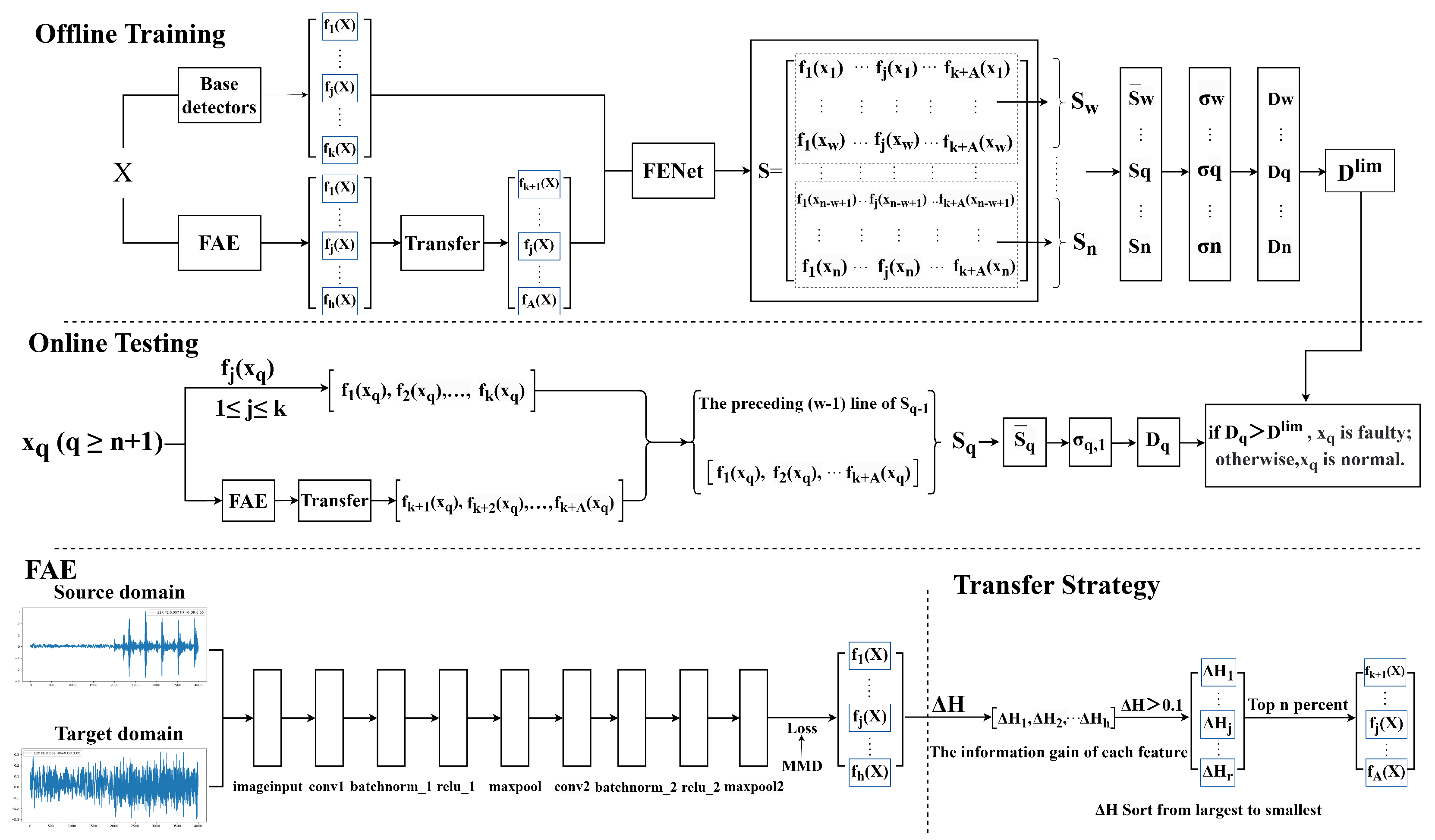
FAENet is proposed for incipient fault detection to address the critical challenge of insufficient cross-domain generalization capacity through a synergistic integration of transfer learning and ensemble learning. As shown in Figure 1, the overall framework of FAENet is given in three components:

(1)

A feature adaptive extractor (FAE) leverages a CNN combined with an MMD [27] to extract domain-invariant features, aligning source and target domain distributions to minimize cross-domain discrepancies.

(2)

An information entropy gain-driven feature screening module dynamically filters redundant features and mitigates negative transfer effects by evaluating the information gain of each feature relative to fault labels, thereby retaining only discriminative features critical for accurate detection.

(3)

A deep multi-feature ensemble framework module integrates raw features from statistical detectors (such as PCA, DPCA, and MDs) with transfer features, constructing an adaptive ensemble matrix. This matrix is further processed via sliding window techniques and singular value decomposition (SVD) to capture multi-scale temporal patterns, ultimately generating a detection index.

The specific implementation details of offline training and online detection are respectively presented in Algorithms 1 and 2.

3.1. Feature Adaptive Extractor (FAE)

Here, a CNN is utilized for feature extraction. The network consists of an input layer and two convolutional and pooling layers that progressively extract and downsample features. Each convolutional layer is followed by batch normalization and ReLU activation layers to improve network stability and nonlinearity. Finally, a fully connected layer generates the output, and the MMD loss layer is employed for optimization, enhancing model performance of the task.

The network architecture includes two convolutional layers. The first convolutional layer employs a kernel size of 64 to capture broad spatial patterns in the input data, which is particularly effective for extracting high-level fault features from complex industrial signals. The second convolutional layer uses a smaller kernel size of 3 to refine these features and capture more localized patterns [28]. This hierarchical approach ensures that both global and local features are effectively captured, enhancing the model’s ability to detect incipient faults. The detailed framework of the FAE is shown in

Table 1. Feature adaptive extraction.

Layer Type	Activation Function	Kernel Size
imageinput	/	/
conv1	/	64
batchnorm_1	ReLU	/
maxpooling	/	/
conv2	/	3
batchnorm_2	ReLU	/
maxpooling	/	/
FC	/	/

.

To minimize the discrepancy between the data distributions of the source and target domains, an MMD is adopted as the loss function for the feature extractor. This maps both the source and target domains into a reproducing kernel Hilbert space (RKHS) [29] using the same mapping and then optimizes the mean discrepancy between the two sets of data in the mapped space to reduce the domain shift.

$$MMD(X,Y)={∥{\displaystyle \frac{1}{n}}\sum _{i=1}^n\varphi \left(x_i\right)-{\displaystyle \frac{1}{m}}\sum _{j=1}^m\varphi \left(y_j\right)∥}_H^2$$

(1)

where H represents the RKHS, $\varphi$ is the feature mapping function that maps the data into the RKHS, and X and Y denote the distributions of the source and target domains, respectively, with n and m representing the sample sizes of the two distributions.

3.2. Information Entropy Gain-Based Feature Screening

During the transfer process, the problem of negative transfer may arise. Therefore, this paper leverages information entropy gain to select features extracted by FAE, aiming to eliminate redundant features that contribute minimally to fault detection as well as transfer features that negatively impact fault detection accuracy. Information gain measures the extent to which a feature contributes to the label. As the information gain value of a feature increases, its contribution to the label also increases. A higher information gain value indicates a more important feature [30].

As stated, the difference in information content is referred to as information gain, which is defined as the difference between the original entropy and the conditional entropy under that feature, representing the amount of information gained. The mathematical expression for information entropy is shown in Equation (2).

$$H\left(X\right)=-\sum _{i=1}^{n}p\left(x_i\right){log}_2\left(p\left(x_i\right)\right)$$

(2)

Assume that the original dataset obtained through multi-feature optimization combination is denoted as D, and A represents the features extracted by the feature extractor. The dataset after adding feature A is denoted as D|A. The information gain is computed by subtracting the entropy of the two datasets. The information obtained is described by Equation (3).

$$\Delta H(D,A)=H\left(D\right)-H(D\mid A)$$

(3)

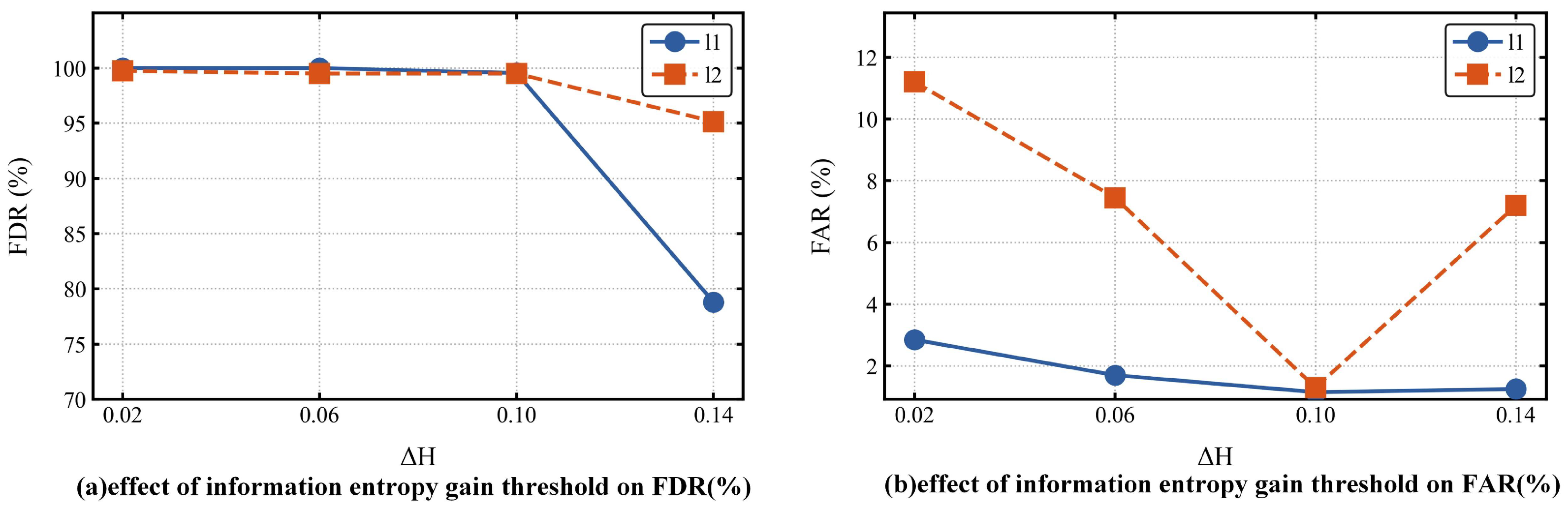
After the computation, the corresponding entropy matrix $\left[\Delta {\mathrm{H}}_1,\Delta {\mathrm{H}}_2,\cdots ,\Delta {\mathrm{H}}_{\mathrm{h}}\right]$ is obtained. To eliminate redundant features with minimal contribution to label detection, features with an information gain $\Delta H$ less than 0.1 are filtered out, resulting in the information entropy matrix after feature selection $\left[\Delta {\mathrm{H}}_1,\Delta {\mathrm{H}}_2,\cdots ,\Delta {\mathrm{H}}_{\mathrm{r}}\right]$ [31].

To prevent the negative transfer effects that may arise from the inclusion of multiple features, which could negatively impact fault detection accuracy, an optimization of different information entropy combinations is performed on the filtered information entropy matrix. By selecting and adding different features iteratively, the information entropy for multiple feature sets is computed and ranked. The top-ranked features are then retained as key features, thereby achieving the purpose of feature selection. Ultimately, the features selected through the information entropy gain-based feature screening $s={\left[f_1\left({\mathbf{x}}_i\right),f_2\left({\mathbf{x}}_i\right),\cdots ,f_A\left({\mathbf{x}}_i\right)\right]}^T\in {\mathbb{R}}^A$ are obtained.

3.3. Deep Multi-Feature Ensemble Framework

Similarly to FENet, various data-driven fault detection methods, such as PCA and DPCA, are employed as base detectors in FAENet. Using these detectors, an original feature ensemble matrix is created. However, this kind of original feature ensemble matrix may contain a large number of redundant features that contribute minimally to the detection task. These features not only increase computational complexity but also introduce noise, thereby reducing model generalization ability. Additionally, FENet fails to effectively handle situations involving the scarcity of failure samples and under cross-domain detection challenges. The selected feature-based information entropy gain-based feature screening is then incorporated into this original matrix, resulting in the final adaptive feature ensemble matrix. The resulting FENet framework, constructed upon this architecture, demonstrates dual capabilities: precise detection of incipient faults under data scarcity conditions and cross-domain fault detection performance. These distinctive characteristics warrant its designation as FAENet in technical nomenclature.

Let the process measurement data be represented by $\mathit{x}\in {\mathbb{R}}^m$, where m denotes the number of sensors corresponding to each sample. The training dataset, consisting of n samples under normal operating conditions, is represented as $\mathit{X}={\left[x_1,x_2,\cdots ,x_n\right]}^T\in {\mathbb{R}}^{n\times m}$. The mapping from the process data x to the corresponding detection metric for each detector is defined as $x\to f\left(x\right)$. For detectors based on multivariate statistical analysis, this function is commonly represented as $f\left(x\right)={∥{\mathit{M}}^T\mathit{x}∥}_2^2$, where M is the linear projection matrix. For a given sample $x_i$, after evaluation by k fundamental detectors, the resulting k detection metrics are compiled into a detection feature vector $s_i={\left[f_1\left({\mathit{x}}_i\right),f_2\left({\mathit{x}}_i\right),\cdots ,f_k\left({\mathit{x}}_i\right)\right]}^T\in {\mathbb{R}}^k$.

Thus, the detection feature vectors corresponding to all training samples $x_i$ (i = 1, 2, …, n) are computed and assembled to represent the input feature matrix S [26]:

$$\mathit{S}=\left[\begin{array}{cccc}{f}_1\left({\mathit{x}}_1\right)& f_2\left({\mathit{x}}_1\right)& \cdots & f_k\left({\mathit{x}}_1\right)\\ f_1\left({\mathit{x}}_2\right)& f_2\left({\mathit{x}}_2\right)& \cdots & f_k\left({\mathit{x}}_2\right)\\ ⋮& ⋮& \ddots & ⋮\\ f_1\left({\mathit{x}}_n\right)& f_2\left({\mathit{x}}_n\right)& \cdots & f_k\left({\mathit{x}}_n\right)\end{array}\right]\in {\mathbb{R}}^{n\times k}$$

(4)

By incorporating the A extracted features into Equation (4), we obtain the proposed adaptive feature matrix:

$$\mathit{S}=\left[\begin{array}{cccccc}{f}_1\left({\mathit{x}}_1\right)& \cdots & f_k\left({\mathit{x}}_1\right)& f_{k+1}\left({\mathit{x}}_1\right)& \cdots & f_{k+A}\left({\mathit{x}}_1\right)\\ f_1\left({\mathit{x}}_2\right)& \cdots & f_k\left({\mathit{x}}_2\right)& f_{k+1}\left({\mathit{x}}_2\right)& \cdots & f_{k+A}\left({\mathit{x}}_2\right)\\ ⋮& \ddots & ⋮& ⋮& \ddots & ⋮\\ f_1\left({\mathit{x}}_n\right)& \cdots & f_k\left({\mathit{x}}_n\right)& f_{k+1}\left({\mathit{x}}_n\right)& \cdots & f_{k+A}\left({\mathit{x}}_n\right)\end{array}\right]\in {\mathbb{R}}^{n\times (k+A)}$$

(5)

The adaptive feature ensemble matrix S obtained is then fed into the feature transformer layer. In each layer, a sliding window technique with a window size of w is applied to the adaptive feature ensemble matrix from Equation (5). This results in a sliding window matrix $S_{p,ki}^i$ with a window width of $w\times h_l$:

$$S_{p,ki}^i=\left[\begin{array}{cccc}{s}_{p,c_{ki}\left(1\right)}^i& s_{p,c_{ki}\left(2\right)}^i& \cdots & s_{p,c_{ki}\left(k+A\right)}^i\\ s_{p+1,c_{ki}\left(1\right)}^i& s_{p+1,c_{ki}\left(2\right)}^i& \cdots & s_{p+1,c_{ki}\left(k+A\right)}^i\\ ⋮& ⋮& \ddots & ⋮\\ s_{p+w-1,c_{ki}\left(1\right)}^i& s_{p+w-1,c_{ki}\left(2\right)}^i& \cdots & s_{p+w-1,c_{ki}\left(k+A\right)}^i\end{array}\right]\in {\mathbb{R}}^{w\times h_l}$$

(6)

Subsequently, the matrix $S_{p,ki}^i$ undergoes standardization processing:

$${\overline{\mathit{S}}}_{p,ki}^i=\left({\mathit{S}}_{p,ki}^i-{\mathbf{1}}_{\omega }^T{\mu }_{p,ki}\right){\Sigma }_{p,ki}^{-1},$$

(7)

where ${\mathbf{1}}_{\mathit{w}}={\left[1,1,\cdots ,1\right]}^T\in {\mathbb{R}}^w$, ${\mu }_{p,ki}\in {\mathbb{R}}^{1\times h_l}$ represents the mean value of the $h_l$ detection features corresponding to the n samples and the diagonal matrix ${\Sigma }_{p,ki}$ represents the standard deviation.

After obtaining the normalized matrix ${\overline{S}}_{p,ki}^i$, the SVD is applied as follows:

$${\overline{S}}_{p,ki}^i=U_{p,ki}^i\sum _{p,ki}^i{\left(V_{p,ki}^i\right)}^T$$

(8)

where $U_{p,ki}^i\in {\mathbb{R}}^{m\times w}$, ${\sum }_{p,ki}^i\in {\mathbb{R}}^{w\times h_l}$, and $V_{p,ki}^i\in {\mathbb{R}}^{h_l\times h_l}$ are the left singular matrix, diagonal matrix of singular values, and right singular matrix. After SVD, the singular values of the matrix are ${\sigma }_{p,ki}^i=\left[{\sigma }_{p,ki}^{i\left(1\right)},{\sigma }_{p,ki}^{i\left(2\right)},\dots ,{\sigma }_{p,ki}^{i\left(h_l\right)}\right]\in {\mathbb{R}}^{1\times h_l}$.

Further, the singular value matrix $V_{ki}^i$ corresponding to the different samples can be obtained:

$${\mathit{V}}_{ki}^i={\left[{\sigma }_{n-n_l+w,k_i}^i,{\sigma }_{n-n_l+w+1,k_i}^i,\cdots ,{\sigma }_{n,k_i}^i\right]}^T$$

(9)

Similarly to the feature transformation layer in [26], then, PCA is performed on each $V_{ki}^i$ to obtain $x_p$ corresponding to the $T^2$ statistics and the Q statistics:

$${\mathit{T}}^i=\left[\begin{array}{ccc}{T}_{n-n_i+w,i,1}^2& \cdots & T_{n-n_i+w,i,C_{m_i}^{h_i}}^2\\ ⋮& \ddots & ⋮\\ T_{n,i,1}^2& \cdots & T_{n,i,C_{m_i}^{h_i}}^2\end{array}\right]$$

(10)

$${\mathit{Q}}^i=\left[\begin{array}{ccc}{Q}_{n-n_i+w,i,1}& \cdots & Q_{n-n_i+w,i,C_{m_i}^{h_i}}\\ ⋮& \ddots & ⋮\\ Q_{n,i,1}& \cdots & Q_{n,i,C_{m_i}^{h_i}}\end{array}\right]$$

(11)

Then, the output of the $(i+1)$th transformer layer is expressed as:

$${\mathit{S}}^{i+1}=\left[{\mathit{T}}^i,{\mathit{Q}}^i\right]\in {\mathbb{R}}^{\left(n_i-w+1\right)\times 2h_i}$$

(12)

In the final ($l^{max}$) feature transformation layer, all output feature matrices corresponding to different sliding window sizes are fused into a large feature matrix based on the sample sampling moments. This fused matrix is denoted as $S_p^o\in {\mathbb{R}}^{n_o\times m_o}$. The matrix $S_p^o$, as the feature matrix of the output feature layer, serves as a crucial foundation for the decision layer.

In the decision layer, the input is the feature matrix $S_p^o$ from the output feature layer. Based on the feature matrix $S_p^o$, a full sliding window is applied along the row direction, with a sliding window size of $w\times m_o$, encompassing all columns of the feature matrix. For the sample $x_q$, the corresponding sliding window matrix is represented as

$${\mathit{S}}_p^o={\left[{\mathit{s}}_{p-w+1}^o,{\mathit{s}}_{p-w+2}^o,\cdots ,{\mathit{s}}_p^o\right]}^T\in {\mathbb{R}}^{w\times m_o}$$

(13)

where $p=n-n_o+w,n-n_o+w+1,...,n$.

Then, $S_p^o$ is normalized to ${\overline{S}}_p^o$. Applying SVD, the singular values are denoted as ${\sigma }_p^o=\left[{\sigma }_1,{\sigma }_2,\cdots ,{\sigma }_{m_o}\right]\in {\mathbb{R}}^{1\times m_o}$.

For the standardized sliding window matrix ${\overline{S}}_p^o$, the corresponding maximum singular value is calculated as ${\sigma }_p^o$, and then the detection index of $x_p$ can be designed as [26]:

$$D_p={∥{\Phi }^{-1}\left({\sigma }_p^o-\kappa \right)∥}_2$$

(14)

where $\kappa$ and $\varphi$ represent the mean and standard deviation of ${\left\{{\sigma }_p^o\right\}}_{n-n_0+w}^n$, respectively.

Given the confidence level, the corresponding control limits of the detection index $D^{lim}$ can be calculated by the empirical method or kernel density estimation (KDE). If $D_p$ exceeds $D^{lim}$, $x_p$ represents the fault data.

Algorithm 1 Offline Training

Input:  Input data X, number of basic detectors k, width of sliding windows w, number of feature transformer layers $l^{max}$, significance level $\alpha$, source domain data $X_s$, target domain data $X_t$. Output:  Control limit $D^{lim}$, detectors ${\left\{f_j\left(x\right)\right\}}_{j=1}^k$, structure of FENet.   1: Construct k detectors as ${\left\{f_j\left(x\right)\right\}}_{j=1}^k$   2: Stack ${\left\{f_j\left(x\right)\right\}}_{j=1}^k$ into S via (1)   3: Features_s = CNN($X_s$)   4: Features_t = CNN($X_t$)   5: MMD_loss = MMD(Features_s, Features_t)   6: Total_loss = Classification_loss + $\lambda$ * MMD_loss   7: Optimizer.minimize(Total_loss)   8: Extract candidate features F = [$f_1$, $f_2$, …, $f_h$] from FAE output   9: Compute information entropy gain $\Delta H(D,f_i)$ for each feature 10: for  $i=1,2,3,\dots ,h$  do 11:     if $\Delta H(D,f_i)\ge 0.1$ then 12:         Add $f_i$ to matrix F_selected 13:     end if 14: end for 15: F_selected = [$f_1$, $f_2$, …, $f_A$] 16: F_selected are ranked in descending order of their information entropy gain 17: if  $l^{max}=0$  then 18:     Set $S^o=S$, proceed to 26 19: else 20:     Set $S^0=S$ 21:     for $l=0,1,2,\dots ,l^{max}-1$ do 22:         Set $h_l$ 23:         Calculate $S^{l+1}=g\left(S^l\right)$ via (6)–(12) as the output feature matrix in the $(l+1)$-th feature transformer layer; 24:     end for 25: end if 26: Obtain feature matrix $S^o$ in the output feature layer 27: for  $p=n-n_o+w,n-n_o+w+1,\dots ,n$  do 28:     Obtain sliding window matrix $S_p^o$ 29:     Normalize $S_p^o$ as ${\overline{S}}_p^o$ 30:     Calculate singular values of ${\overline{S}}_p^o$ as ${\sigma }_p^o$ 31: end for 32: Calculate detection indices ${\left\{D_p\right\}}_{p=n-n_o+w}^n$ via Equation (14) 33: Compute $D^{lim}$ with significance level $\alpha$

Algorithm 2 Online Detection

Input:  New sample $x_p(p\ge n+1)$, control limit $D^{lim}$, detectors ${\left\{f_j\left(x\right)\right\}}_{j=1}^k$, structure of FENet, real-time data stream $x_{new}$, trained FAENet model. Output:  Status (normal or faulty) of $x_p$.   1: Obtain feature vector $s_p$ for new sample $x_p$   2: $s_{qnew}$ = FAE($x_{new}$)   3: for  $i=1,2,3,\dots ,h$  do   4:     if $\Delta H(s_q,s_{qnew}\left[i\right])\ge 0.1$ then   5:         Add $s_{qnew}\left[i\right]$ to $s_q$   6:     end if   7: end for   8: if  $l^{max}=0$  then   9:     Set $s_p^o=s_p$ 10: else 11:     Set $s_p^0=s_p$ 12:     Update $S_p^0$ with $s_p^0$ and $S_{p-1}^0$ 13:     for $l=0,1,2,\dots ,l^{max}-1$ do 14:         Calculate $s_p^{l+1}$ in the output of the $(l+1)$-th feature transformer layer 15:     end for 16: end if 17: Update $S_p^o$ with $s_p^o$ and $S_{p-1}^o$ in the output feature layer 18: Normalize $S_p^o$ as ${\overline{S}}_p^o$ 19: Calculate singular values of ${\overline{S}}_p^o$ as ${\sigma }_p^o$ 20: Compute detection index $D_p$ via (14) 21: Determine status of $x_p$ according to $D_p$ and $D^{lim}$

4. Simulations

4.1. Parameter Setting

To enhance computational efficiency while preserving critical fault-related information, the sliding window block size in FAENet is adaptively configured based on the dimensions of the feature matrix. For a given feature matrix $S\in {\mathbb{R}}^{n\times k}$, the default window length is defined as $h_l=⌊0.95k⌋$, where $\lfloor ·\rfloor$ represents the floor function. This parameter selection aims to minimize the combinatorial complexity arising from column-wise sampling. Specifically, the number of possible combinations for selecting $h_l$ columns from k candidates is calculated as:

$$C_k^{h_l}={\displaystyle \frac{k!}{h_l!\left(k-h_l\right)!}}$$

(15)

Reducing $h_l$ excessively increases computational demands exponentially. For example, when $k=10$, the values $h_l=9,8$, and 7 correspond to $C_{10}^9=10,C_{10}^8=45$, and $C_{10}^7=120$, respectively. Thus, $h_l=\lfloor 0.95\times 10\rfloor =9$ achieves an optimal trade-off between computational efficiency and depth information extraction.

In the feature transformation stage, singular value matrices derived from sliding window operations are decomposed into the $T^2$ statistics and the Q statistics using PCA. The cumulative percentage variance threshold, which governs the separation of principal and residual subspaces, is uniformly set to 90% to retain significant process variations. Finally, in the decision layer, the detection index is formulated based on the L2-norm (p = 2) of normalized singular values. This choice aligns with practical requirements for fault detection sensitivity.

4.2. The Sensitivity Analysis of Information Entropy Gain Threshold

To validate the robustness of the information entropy gain threshold ($\Delta H=0.1$), a sensitivity analysis was conducted by testing alternative thresholds on the TEP dataset. Alternative thresholds (0.02, 0.06, 0.1, 0.14) were systematically examined within the interval [0.02, 0.14] using a step size of 0.04, with corresponding average FDR and FAR recorded under different thresholds.

As illustrated in Figure 2, the threshold $\Delta H=0.1$ achieves optimal balance between high FDR (99.5%) and low FAR (1.15%). Thresholds below 0.1 marginally improved FDR but substantially increased FAR due to excessive retention of redundant features, elevating overfitting risks. Conversely, thresholds exceeding 0.1 caused significant FDR deterioration despite stable FAR performance, attributable to excessive feature elimination that compromised critical commonality information across fault patterns.

The sensitivity analysis confirms that the 0.1 threshold delivers optimal performance across datasets by balancing feature preservation and overfitting mitigation. While the information entropy gain threshold $\Delta H=0.1$ ensures the retention of only the most discriminative features, its universal applicability across diverse industrial process scenarios remains limited. To address this problem, FAENet performs iterative optimization after initial feature selection. Features are ranked in descending order of their information entropy gain. The framework then progressively selects the top n% features (n increasing with predetermined step size) through multiple iterations until the transferred features’ information entropy gain reaches its maximum. This adaptive mechanism significantly enhances the robustness of the FAENet framework when handling heterogeneous industrial environments.

4.3. Tennessee Eastman Process

4.3.1. TEP Dataset

The TEP serves as an open simulation platform for chemical processes, specifically designed by the Eastman chemical company to model a chemical combination reaction process [32]. The structure of the TEP system is shown in Figure 3. The data generated from the TEP exhibit dynamic, strongly coupled, and highly nonlinear characteristics, making them widely utilized for validating the effectiveness of fault detection methods. It encompasses 53 observable variables (22 continuous variables, 19 process variables, and 12 operational variables). Furthermore, the TEP includes 21 distinct types of faults; among these are fault 3 (a step fault), fault 9 (a random variable fault), and fault 15 (a stuck valve fault). These categories of faults are commonly regarded as typical incipient faults by numerous academicians; due to the presence of feedback control mechanisms within the system, these incipient faults exert relatively minimal influence on overall process. For instance, both the mean and variance of their corresponding observable variables demonstrate negligible changes before and after the occurrence of these faults. This characteristic is a key reason why faults 3, 9, and 15 are difficult to detect.

In the simulations, both the training and testing phases are conducted over a duration of 200 h with a sampling interval set at three minutes. In this context, dataset d00 represents normal process data used for training models; datasets d01–d21 consist of fault data employed to assess detector performance. Within each test dataset introduced after the first hundred hours into operation, specifically starting from sample number 2001, the initial segment comprising the first 2000 samples consists solely of normal data prior to introducing any faults thereafter. Subsequently calculated based on the final 2000 samples collected during testing are the FDRs. Notably recognizing that d00 constitutes normal process data allows us to interpret its FDR concerning fault 00 as indicative of false alarm rate (FAR). In the TEP dataset, faults are introduced individually, meaning that each fault occurs independently without overlapping with other faults. This design allows for the evaluation of fault detection methods under isolated fault conditions, ensuring that the performance metrics reflect the ability to detect specific fault types without interference from concurrent faults.

4.3.2. Compared Methods

This paper focuses on the cross-domain detection issue where there is no training data of the target domain faults and puts forward distinct fault detection thoughts. Based on the current mainstream cross-domain fault detection methods, this paper implements the following four comparative methods in the TEP. Meanwhile, all the compared methods possess similar network configurations to the proposed one.

(1)

TCA (Transfer Component Analysis) [33]: This method is employed in the context of domain adaptation. It identifies a set of transfer components within an RKHS, such that when domain data are projected onto the latent space spanned by these transfer components, the distance between different domains can be effectively reduced.

(2)

JDA (Joint Distribution Adaptation) [34]: Joint distribution adaptation involves concurrently adjusting both marginal and conditional distributions through a principled dimensionality reduction process.

(3)

DANNs (Domain-Adversarial Neural Networks) [35]: Domain-adversarial neural networks are designed to simultaneously learn the classifier, feature extractor, and domain discriminator. By minimizing FAR while maximizing FDR, this approach facilitates the extraction of meaningful features.

(4)

DTL (Deep Transfer Learning) [22]: Deep transfer learning leverages deep learning techniques to implement transfer learning strategies. Typically, it involves utilizing deep neural networks to learn feature representations from the source domain and subsequently applying these learned features to enhance performance on tasks within the target domain.

4.3.3. Experimental Results in TEP Dataset and Performance Analysis

In this section, fault 2 (step-type perturbation in reactor cooling water flow) and fault 4 (step-type variation in condenser temperature) are designated as the source domains for feature adaptive extraction, as their distinct temporal patterns and higher signal amplitudes (such as abrupt changes in XMEAS(9) and XMV(12)) enable robust baseline detection. These source faults contrast sharply with the target domain faults such as faults 3, 5, 9, 15, 16, and 21 in the TEP, which encompass diverse incipient mechanisms as detailed in

Table 2. Details of transfer learning tasks.

Source → Target	Source Fault Type	Target Fault Type
Fault 2 → fault 3	Step	Step
Fault 4 → fault 5	Step	Step
Fault 2 → fault 9	Step	Random variation
Fault 2 → fault 15	Step	Sticking
Fault 4 → fault 16	Step	Unknown
Fault 4 → fault 21	Step	Constant position

. The process of feature adaptive extraction and information entropy gain-based feature screening is conducted without utilizing the fault information from the target domain. Transfer features mined during cross-domain transfer are integrated with the base detectors of PCA, DPCA, and MDs to construct a new feature ensemble matrix for subsequent fault detection.

The fault detection results obtained using TCA, JDA, DANN, DTL, and FAENet are tested and presented in

Table 3. The FDRs (%) of TCA, JDA, DANN, DTL, and FAENet for the TEP.

Source → Target	TCA	JDA	DANN	DTL	FAENet
					l1	l2
Fault 2 → fault 3	2.25	0.225	45.3	44.65	99.45	99.3
Fault 4 → fault 5	0.4	0	31.65	31.05	99.9	99.8
Fault 2 → fault 9	3.3	1.1	42.85	41.05	98.85	98.6
Fault 2 → fault 15	1.1	0	35.3	34	99.55	99.5
Fault 4 → fault 16	0.7	0	35.15	35.20	99.5	99.7
Fault 4 → fault 21	0.9	0	33.65	32.95	99.45	99.55
Average	1.44	0.23	37.32	36.49	99.45	99.41

. The sliding window width for FAENet is set to 150. The significance level of each base detector is established at 1%, while control limits are calculated using KDE. All the compared methods possess similar network configurations to the proposed one. As illustrated in Table 3, both TCA and JDA demonstrate ineffectiveness in detecting faults 3, 5, 9, 15, 16, and 21; their average FDR stands at a mere 0.84%. Similarly poor performance is observed with DANN and DTL regarding these same faults; they achieve an average FDR of only 36.91%. In contrast to these methods, FAENet can achieve an FDR of 99.45% in l1 and achieve an FDR of 99.41% in l2. To further analyze the impact of feature adaptive extraction and information entropy gain-based feature screening on performance outcomes, we employ an effective visualization technique known as t-SNE (t-distributed Stochastic Neighbor Embedding) that maps samples from high-dimensional original feature space into a two-dimensional representation space. High-level representations within source domains 2 and 5 exhibit well-defined clustering patterns, with data samples under varying conditions distinctly separated. The clustering serves as a foundation for accurate detection of faults within the source domain. Conversely, as depicted in Figure 4, high-level representations corresponding to target domains 3, 9, and 15 reveal poor clustering characteristics; data samples across different conditions appear intermixed. The lack of separation constitutes a significant factor contributing to challenges associated with detecting such incipient faults effectively. After feature adaptive extraction and information entropy gain-based feature screening, the distribution differences between the source domain and the target domain are significantly reduced, resulting in closer marginal distributions. The data samples under different conditions in the target domain are effectively separated, which greatly enhances cross-domain fault detection capabilities.

In addition, the FDRs of the ensemble strategies are presented in

Table 4. The FDRs (%) of various ensemble methods for the TEP.

Fault	Averaging	Voting	Bayes Inference	FENet		FAENet
				l1	l2	l1	l2
00	0.85	0	0.6	1.4	4.1	1.2	0.85
03	28.4	0.15	16.9	93.25	91.5	99.45	99.3
05	31	0.1	13.3	55.65	81.05	99.9	99.8
09	27.5	0.3	17.8	94.7	94.25	98.85	98.6
15	24.65	0.05	11.6	61.6	80.8	99.55	99.5
16	25	0.05	8.05	72.2	85.55	99.5	99.7
21	30.8	0.4	14	72.6	81.25	99.45	99.55
Average	27.9	0.18	13.61	75	85.74	99.45	99.41

. In the experiment, the base detectors utilized for FENet are PCA, DPCA, and MDs. The sliding window width for both FENet and FAENet is set to 150. The significance level of each base detector is established at 1%, while control limits are computed using KDE. The average FDRs of FENet and FAENet surpass those achieved through averaging, voting, and Bayesian inference strategies by more than 56% when applied to faults 3, 5, 9, 15, 16, and 21. When comparing the average FDRs between FENet and FAENet, it is evident that FAENet demonstrates superior fault detection capabilities; specifically, its FDR is 24.45% higher than that of FENet in l1 and 13.67% higher in l2. Notably, for faults 5 and 15, the detection performance of FAENet exceeds that of FENet by an impressive margin 41.1% higher in l1 and 18.7% higher in l2. When it comes to faults 5, 15, and 21, FAENet can achieve an FDR of 99% in l2, while the FDRs of FENet are lower than 85%. Furthermore, FAENet achieves an outstanding performance with all its FDRs exceeding 99.4% for faults 3, 5, 9, 15, 16, and 21, thereby illustrating its proficiency in extracting common features from fault signals. For a more detailed analysis, the detection results for faults 3, 9, and 15 as obtained from both FENet and FAENet in l1 are depicted in Figure 5, respectively. The statistics of FAENet exhibit a rapid increase upon fault occurrence; this sensitive response leads to a higher FDR compared to FENet, demonstrating the efficiency of FAENet for incipient fault detection.

As shown in Figure 5a–c, FENet exhibits delayed responses to faults 3, 9, and 15, with detection indices ($D_p$) exceeding the control limit ($D^{lim}$) only after multiple sampling intervals. In contrast, Figure 6a–c demonstrate that FAENet achieves rapid fault identification, with $D_p$ surging immediately post-fault occurrence (sample index 2001). This sensitivity is attributed to the domain-invariant feature migration of FAENet, which enhances the feature representation of incipient fault signals. Similarly, Figure 6a–c reveal FENet’s limited capability in detecting faults 5, 16, and 21 under l1, as evidenced by fluctuating $D_p$ values near the control limit. FAENet Figure 6d–f resolve this issue through entropy-based feature screening, stabilizing $D_p$ trajectories and achieving near-perfect FDRs (Table 3). For l2 (Figure 7 and Figure 8), the additional feature transformation layers enhance the extraction of multi-scale temporal patterns. While FENet’s performance degrades slightly in Figure 7a–c due to accumulated redundant features from iterative transformations, FAENet maintains robust detection in Figure 7d–f by adaptively filtering irrelevant transfer features through entropy-based screening. Notably, Figure 8f highlights FAENet’s superiority in fault 21 detection, where $D_p$ remains consistently above $D^{lim}$.

4.4. CWRU

4.4.1. Experimental Setup of CWRU Dataset

The rolling bearing dataset utilized in this study is sourced from the bearing data center at Case Western Reserve University [36]. The experimental setup is depicted in Figure 9. This publicly available dataset has been widely employed in related research endeavors. In this study, 2000 consecutive sampling points of normal operating data were extracted from the dataset firstly, followed by an equivalent sequence length for each fault category. These paired temporal segments, representing both normal and anomalous system states, were subsequently visualized through time-series analysis as illustrated in Figure 10. Considering the substantial impact of fault signals on process data integrity, we identified an incipient fault through time-series analysis under controlled parameters: a 12 kHz sampling frequency at the fan-end bearing and a drive-end bearing defect diameter of 0.007 inches. The investigation specifically targeted outer raceway failures at the 3 o’clock orientation, operationally designated as “12K FE 0.007 OR 3:00”. Additionally, “12K FE 0.007 OR 6:00” serves as our source domain; feature adaptive extraction and information entropy gain-based feature screening processes are conducted under varying operational conditions (motor loads of 0 and 1) to construct a feature ensemble matrix for subsequent fault detection tasks.

4.4.2. Experimental Results in CWRU Dataset and Performance Analysis

The parameter settings of the model are consistent with those outlined in Section 4.1 of the TEP simulation. The simulation results for CWRU are presented in

Table 5. The FDRs (%) of TCA, JDA, DANN, DTL, and FAENet for CWRU.

Source→Target	TCA	JDA	DANN	DTL	FAENet
					l1	l2
OR 6:00→OR 3:00 (HP = 0)	28	24.15	69.95	36	99.95	99.95
OR 6:00→OR 3:00 (HP = 1)	27.75	23.35	38.3	33.85	98.85	99.15
Average	27.875	23.75	54.375	34.925	99.4	99.55

. The performance of TCA, JDA, DANN, and DTL in detecting fault “12K FE 0.007 OR 3:00” is suboptimal, yielding average FDRs of only 27.875%, 23.75%, 54.375%, and 34.925%, respectively. In contrast, FAENet demonstrates a significant improvement over existing cross-domain fault detection in detecting fault “12K FE 0.007 OR 3:00”, achieving average FDRs of 99.4% and 99.95% in l1 and l2. For a more detailed analysis, the detection results for HP = 0 and HP = 1 as obtained from both FENet and FAENet are depicted in Figure 11 and Figure 12, respectively. The statistics of FAENet exhibit a rapid increase upon fault occurrence; this sensitive response leads to a higher FDR compared to FENet, demonstrating the efficiency of FAENet for incipient fault detection.

Figure 9. Experimental setup of CWRU [36].

Figure 9. Experimental setup of CWRU [36].

Figure 10. Time series curves for faults.

Figure 10. Time series curves for faults.

Figure 11. Detection performances of FENet and FAENet for HP = 0.

Figure 11. Detection performances of FENet and FAENet for HP = 0.

Figure 12. Detection performances of FENet and FAENet for HP = 1.

Figure 12. Detection performances of FENet and FAENet for HP = 1.

4.5. Time Complexity and Computational Overhead

4.5.1. Time Complexity

Although FAENet demonstrates excellent performance in cross-domain fault detection, its time complexity remains a critical consideration. The FAENet framework comprises three principal components: FAE, information entropy gain-based feature screening, and a deep multi-feature ensemble framework. The time complexity of FAE primarily stems from convolutional layers in the neural network and MMD loss computation. As shown in Table 1, the network architecture contains two convolutional layers with kernel sizes of 64 and 3, respectively. For input data containing n samples and m features, the time complexity of the first convolutional layer is:

$$O(n·m·64·C_1)$$

(16)

The second convolutional layer exhibits a time complexity of:

$$O(n·C_1·64·r)$$

(17)

where $C_1$ denotes the output channels of the first convolutional layer and r represents the number of domain-invariant features extracted by FAE.

The MMD loss calculation introduces additional time complexity:

$$O({(n+n)}^2·m)$$

(18)

Information entropy gain-based feature screening primarily involves entropy and conditional entropy computations. The total complexity for evaluating all features across samples is $O(r·n)$. The iterative feature selection process, which sorts features by entropy gain and progressively selects the top p% of features with optimized step size, reaches a maximum complexity of $O(r^2·n)$ when considering a complete traversal of domain-invariant features.

The deep multi-feature ensemble framework consists of four components: input feature layer, feature transformer layer, output feature layer, and decision layer. The input feature layer integrates outputs from multiple parallel detectors (PCA, DPCA, MDs) and domain-invariant features, with complexity dominated by:

$$O(n·m·64·C_1+n·C_1·3·r+{\left(2n\right)}^2·m+r^2·n)$$

(19)

The feature transformer layer employs sliding windows and SVD for deep feature extraction. For window dimensions $w\times h_l$, the per-window SVD complexity is $O\left(2w{h}_l^2\right)$, followed by PCA computation at $O\left(4h_l^2\right)$. Considering $C_m^{h_l}$ possible combinations, the layer complexity becomes:

$$O\left(2C_m^{h_l}w{h}_l^2+4C_m^{h_l}{h}_l^2\right)$$

(20)

Aggregated across $l_{\max }$ transformer layers, the total time complexity is:

$$O\left(\sum _{l=0}^{l_{max}-1}\left(2C_m^{h_l}w{h}_l^2+4C_m^{h_l}{h}_l^2\right)\right)$$

(21)

The decision layer utilizes sliding window SVD with complexity $O\left(2w{h}_l^2\right)$. The overall FAENet complexity can be expressed as:

$$O\left(64nm{C}_1+3n{C}_{1}r+4n^{2}m+n{r}^2+\sum _{l=0}^{l_{max}-1}\left(2C_m^{h_l}w{h}_l^2+4C_m^{h_l}{h}_l^2+2w{h}_l^2\right)\right)$$

(22)

The time complexity of FAENet is primarily determined by its network architecture and the number of feature transformer layers. Particularly when the number of feature transformer layers $l_{\max }$ increases, the time complexity escalates significantly. In contrast, PCA, DPCA, and MD exhibit lower complexity, whereas TCA and JDA demonstrate higher complexity, especially with large sample sizes n. The complexity of DANN and DTL depends on their network depth and training epochs, typically falling between PCA and TCA. FAENet achieves superior detection performance through partial computational efficiency sacrifice, enabling the detection of incipient faults undetectable by conventional methods like PCA, TCA, and JDA. The comparison of time complexity for various methods is presented in

Table 6. The time complexity of TCA, JDA, DANN, DTL, and FAENet for the TEP.

Model	Time Complexity
PCA	O$(m^3$)
DPCA	O$(4t^2{m}^2$)
MD	O$(m^3$)
TCA	O$(n^3$)
JDA	O$(n^3+d^3$)
DANN	O$(N_{\mathrm{epoch}}·n·d^2$)
DTL	O$(N_{\mathrm{epoch}}·n·d^2$)
FAENet	O$(64nm{C}_1+3n{C}_{1}r+4n^{2}m+n{r}^2+{\sum }_{l=0}^{l_{max}-1}\left(2C_m^{h_l}w{h}_l^2+4C_m^{h_l}{h}_l^2+2w{h}_l^2\right))$

. This advantage makes it particularly suitable for high-precision industrial scenarios requiring sensitivity to progressive faults. Practical implementation requires careful selection of feature transformer layers and sliding window size based on task requirements and computational resource constraints to achieve an optimal balance between detection performance and computational efficiency.

4.5.2. Computational Overhead

To further evaluate the computational efficiency of FAENet, the runtime of FAENet was recorded and comparative analyses were conducted with TCA, JDA, DANN, and DTL. Experimental results demonstrate that FAENet achieves an average runtime of 95.353 s on the TEP dataset. While TCA and JDA maintain high computational efficiency, they exhibit limited capability in detecting incipient faults (faults 3, 5, 9, 15, 16, and 21 in the TEP). Notably, FAENet significantly enhances FDR while maintaining comparable computational efficiency to DANN and DTL. These findings indicate that FAENet not only delivers superior detection accuracy but also demonstrates promising computational performance for practical applications. The comparison of computational overhead for each model is presented in

Table 7. The computational overhead of TCA, JDA, DANN, DTL, and FAENet for the TEP.

Model	Time (s)	FDR (%)
TCA	23.419	1.1
JDA	65.672	0
DANN	97.964	35.3
DTL	79.513	34
FAENet	98.353	99.5

.

5. Discussion

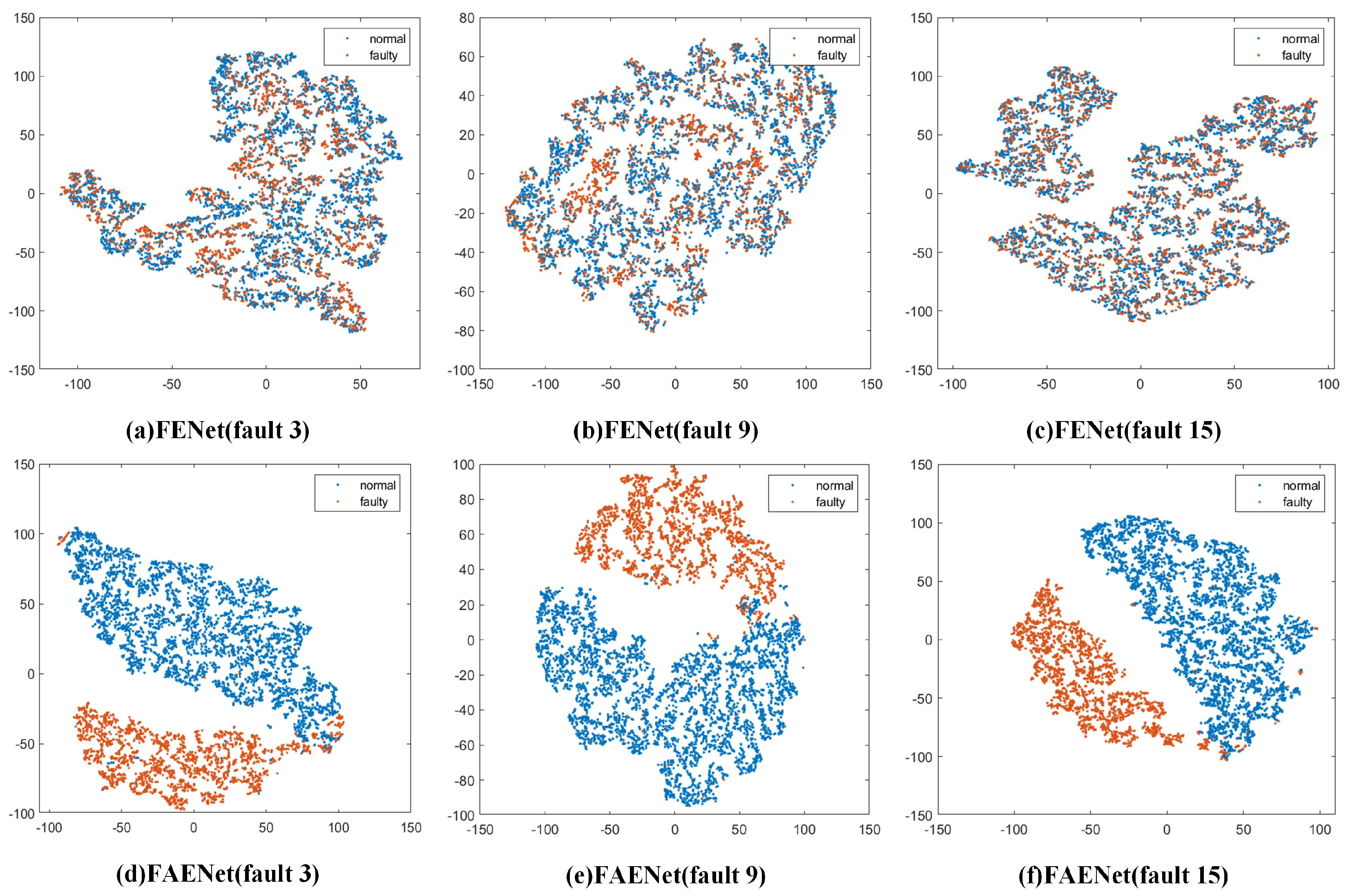
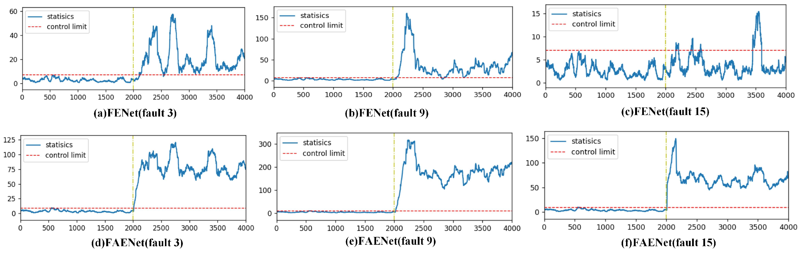
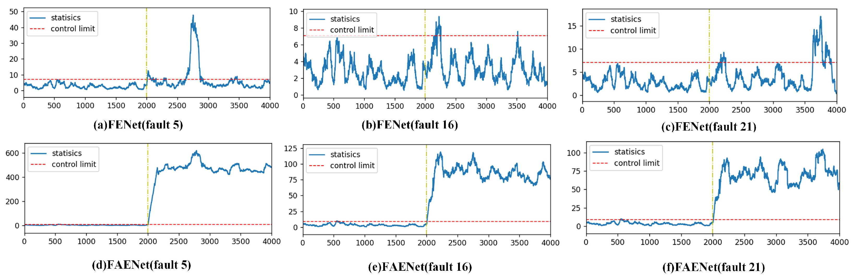
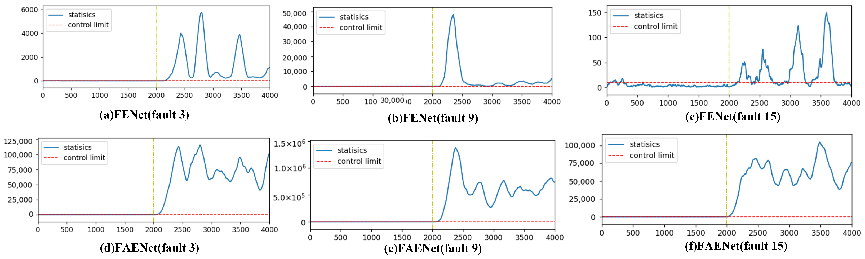
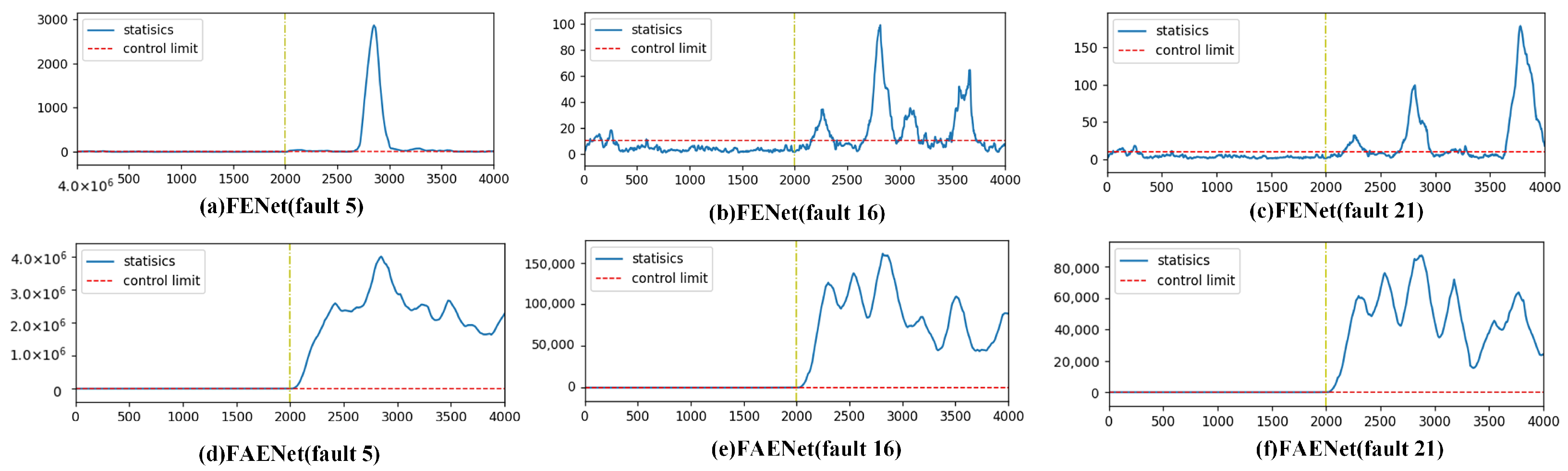
Despite advancements in fault detection technologies, a critical challenge persists: the insufficient cross-domain generalization capacity of existing methods for incipient faults. Traditional approaches, including deep learning frameworks, exhibit limited adaptability under distribution shifts across operational domains. For instance, detecting notoriously challenging TEP faults 3, 9, and 15, even with FENet, remains inefficient due to misaligned feature distributions between the source and target domains. To address this, we integrate transfer learning into the ensemble framework. Through feature adaptive extraction and information entropy gain-based feature screening, FAENet significantly reduces domain discrepancies, aligns marginal distributions, and enhances detection robustness in cross-domain scenarios.

As the number of transformation layers increases, the computational cost of FENet significantly rises due to the increased computational load of SVD. The main contribution of the proposed FAENet method lies in effectively integrating transfer learning into the ensemble learning framework. This method enables successful detection of incipient faults 3, 5, 9, 15, 16, and 21 in the TEP with fewer transformation layers. Therefore, when facing the detection of incipient faults, FAENet proves to be a powerful tool for intelligent fault detection, offering promising applications in practical mechanical detection.

However, in the proposed deep network framework, PCA is employed for feature transformation in the transformation layer. Given the diversity of detection methods, the feature transformer layer should not be limited to PCA; instead, various detectors can be utilized for feature transformation to extract deeper fault detection information. Furthermore, as the dataset grows, the deep network framework can be enhanced into a distributed structure to improve its capacity for handling large-scale data.

While the proposed FAENet demonstrates significant efficacy in detecting single-fault scenarios, the potential for multiple concurrent faults in industrial systems warrants further investigation. In cases where multiple faults occur simultaneously, the superposition of fault signals can amplify the overall impact on system data. This amplification often leads to more pronounced changes in the mean and variance of relevant process variables, potentially enhancing fault detectability. However, the interaction between multiple faults may also introduce complex nonlinearities that challenge traditional detection methods. Future research should explore the performance of FAENet in multi-fault scenarios, particularly focusing on its ability to distinguish and identify individual faults within composite signals. This investigation would provide valuable insights into the method’s robustness and applicability in real-world industrial settings where multiple faults may co-occur.

6. Conclusions

In this paper, FAENet based on a deep learning framework is proposed for incipient fault detection. To improve the cross-domain generalization capacity of FENet while effectively mitigating discrepancies in data distribution between the source domain and target domain, a feature adaptive extractor is developed. Subsequently, information entropy gain-based feature screening is proposed to eliminate redundant features that contribute minimally to fault detection as well as transfer features that negatively affect FDR; this approach facilitates enhanced fault detection. In the simulations, the FDR of FAENet improved by 13.67% and 5.59%, correspondingly, for TEP and CWRU compared to FENet, thereby demonstrating the efficacy of the proposed method.

However, as industrial systems grow increasingly complex, future research should further explore multimodal fusion techniques to enhance the model’s feature representation capability for incipient fault patterns by integrating multi-source heterogeneous data (such as sensor measurements, visual inputs, and time-series signals). Concurrently, combining parallel computing and distributed training strategies could optimize computational efficiency and scalability for industrial big-data scenarios, thereby addressing real-time monitoring demands. Moreover, adaptive modeling frameworks should be developed to capture the time-varying characteristics of dynamic industrial processes, improving the model’s robustness and real-time responsiveness under non-stationary conditions. Advances in these directions will propel intelligent fault detection toward greater efficiency and generalizability, ultimately providing more comprehensive safeguards for industrial safety and reliability.

References

1. Venkatasubramanian, V.; Rengaswamy, R.; Yin, K.; Kavuri, S.N. A review of process fault detection and diagnosis: Part I: Quantitative model-based methods. Comput. Chem. Eng. 2003, 27, 293–311. [Google Scholar] [CrossRef]
2. Qin, S.J. Statistical process monitoring: Basics and beyond. J. Chemom. 2003, 17, 480–502. [Google Scholar] [CrossRef]
3. Geladi, P.; Kowalski, B.R. Partial least-squares regression: A tutorial. Anal. Chim. Acta 1986, 185, 1–17. [Google Scholar] [CrossRef]
4. Ku, W.; Storer, R.H.; Georgakis, C. Disturbance detection and isolation by dynamic principal component analysis. Chemom. Intell. Lab. Syst. 1995, 30, 179–196. [Google Scholar] [CrossRef]
5. Lee, J.M.; Yoo, C.K.; Choi, S.W.; Vanrolleghem, P.A.; Lee, I.B. Nonlinear process monitoring using kernel principal component analysis. Chem. Eng. Sci. 2004, 59, 223–234. [Google Scholar] [CrossRef]
6. Kaspar, M.H.; Ray, W.H. Dynamic PLS modelling for process control. Chem. Eng. Sci. 1993, 48, 3447–3461. [Google Scholar] [CrossRef]
7. Rosipal, R.; Trejo, L.J. Kernel partial least squares regression in reproducing kernel Hilbert space. J. Mach. Learn. Res. 2001, 2, 97–123. [Google Scholar]
8. Qiu, S.H.; Cui, X.P.; Ping, Z.W.; Shan, N.L.; Li, Z.; Bao, X.Q.; Xu, X.H. Deep learning techniques in intelligent fault diagnosis and prognosis for industrial systems: A review. Sensors 2023, 23, 1305. [Google Scholar] [CrossRef]
9. LeCun, Y.; Bottou, L.; Bengio, Y.; Haffner, P. Gradient-based learning applied to document recognition. Proc. IEEE 1998, 86, 2278–2324. [Google Scholar] [CrossRef]
10. Hochreiter, S. Long Short-term Memory. Neural Comput. 1997, 9, 1735–1780. [Google Scholar] [CrossRef]
11. Hinton, G.E.; Salakhutdinov, R.R. Reducing the dimensionality of data with neural networks. Science 2006, 313, 504–507. [Google Scholar] [CrossRef] [PubMed]
12. Hinton, G.E.; Osindero, S.; Teh, Y.W. A fast learning algorithm for deep belief nets. Neural Comput. 2006, 18, 1527–1554. [Google Scholar] [CrossRef] [PubMed]
13. Goodfellow, I.; Bengio, Y.; Courville, A. Deep Learning; MIT Press: Cambridge, MA, USA, 2016. [Google Scholar]
14. Matania, O.; Dattner, I.; Bortman, J.; Kenett, R.S.; Parmet, Y. A systematic literature review of deep learning for vibration-based fault diagnosis of critical rotating machinery: Limitations and challenges. J. Sound Vib. 2024, 590, 118562. [Google Scholar] [CrossRef]
15. Pan, S.J.; Yang, Q. A survey on transfer learning. IEEE Trans. Knowl. Data Eng. 2009, 22, 1345–1359. [Google Scholar] [CrossRef]
16. Yang, D.L.; Zhang, W.B.; Jiang, Y.Z. Mechanical fault diagnosis based on deep transfer learning: A review. Meas. Sci. Technol. 2023, 34, 112001. [Google Scholar] [CrossRef]
17. Shao, S.Y.; McAleer, S.; Yan, R.Q.; Baldi, P. Highly accurate machine fault diagnosis using deep transfer learning. IEEE Trans. Ind. Inform. 2018, 15, 2446–2455. [Google Scholar] [CrossRef]
18. Zhang, R.; Tao, H.Y.; Wu, L.F.; Guan, Y. Transfer learning with neural networks for bearing fault diagnosis in changing working conditions. IEEE Access 2017, 5, 14347–14357. [Google Scholar] [CrossRef]
19. Wen, L.; Gao, L.; Li, X.Y. A new deep transfer learning based on sparse auto-encoder for fault diagnosis. IEEE Trans. Syst. Man Cybern. Syst. 2017, 49, 136–144. [Google Scholar] [CrossRef]
20. Wang, J.J.; Zhao, R.; Gao, R.X. Probabilistic transfer factor analysis for machinery autonomous diagnosis across various operating conditions. IEEE Trans. Instrum. Meas. 2020, 69, 5335–5344. [Google Scholar] [CrossRef]
21. Long, M.S.; Cao, Y.; Wang, J.M.; Jordan, M.I. Learning transferable features with deep adaptation networks. Proc. Int. Conf. Mach. Learn. 2015, 37, 97–105. [Google Scholar]
22. Lu, W.N.; Liang, B.; Cheng, Y.; Meng, D.S.; Yang, J.; Zhang, T. Deep model based domain adaptation for fault diagnosis. IEEE Trans. Ind. Electron. 2016, 64, 2296–2305. [Google Scholar] [CrossRef]
23. Li, J.P.; Huang, R.Y.; He, G.L.; Liao, Y.X.; Wang, Z.; Li, W.H. A two-stage transfer adversarial network for intelligent fault diagnosis of rotating machinery with multiple new faults. IEEE/ASME Trans. Mechatron. 2020, 26, 1591–1601. [Google Scholar] [CrossRef]
24. Zhang, Z.W.; Chen, H.H.; Li, S.M.; An, Z.H.; Wang, J.R. A novel geodesic flow kernel based domain adaptation approach for intelligent fault diagnosis under varying working condition. Neurocomputing 2020, 376, 54–64. [Google Scholar] [CrossRef]
25. An, Z.H.; Li, S.M.; Wang, J.R.; Xin, Y.; Xu, K. Generalization of deep neural network for bearing fault diagnosis under different working conditions using multiple kernel method. Neurocomputing 2019, 352, 42–53. [Google Scholar] [CrossRef]
26. Liu, D.; Wang, M.; Chen, M. Feature Ensemble Net: A Deep Framework for Detecting Incipient Faults in Dynamical Processes. IEEE Trans. Ind. Inform. 2022, 18, 8618–8628. [Google Scholar] [CrossRef]
27. Gretton, A.; Borgwardt, K.M.; Rasch, M.J.; Schölkopf, B.; Smola, A. A kernel two-sample test. J. Mach. Learn. Res. 2012, 13, 723–773. [Google Scholar]
28. Li, J.; Huang, R.; He, G.; Wang, S.; Li, G.; Li, W. A deep adversarial transfer learning network for machinery emerging fault detection. IEEE Sens. J. 2020, 20, 8413–8422. [Google Scholar] [CrossRef]
29. Berlinet, A.; Thomas-Agnan, C. Reproducing Kernel Hilbert Spaces in Probability and Statistics; Springer: Heidelberg, Germany, 2011. [Google Scholar]
30. Jia, N.; Huang, W.; Cheng, Y.; Ding, C.; Wang, J.; Shen, C. A cross-domain intelligent fault diagnosis method based on multi-source domain feature adaptation and selection. Meas. Sci. Technol. 2024, 35, 046108. [Google Scholar] [CrossRef]
31. Luo, C.; Li, T.; Chen, H.; Lv, J.; Yi, Z. Fusing entropy measures for dynamic feature selection in incomplete approximation spaces. Knowl.-Based Syst. 2022, 252, 109329. [Google Scholar] [CrossRef]
32. Bathelt, A.; Ricker, N.L.; Jelali, M. Revision of the Tennessee Eastman Process Model. IFAC-PapersOnLine 2015, 48, 309–314. [Google Scholar] [CrossRef]
33. Pan, S.J.; Tsang, I.W.; Kwok, J.T.; Yang, Q. Domain adaptation via transfer component analysis. IEEE Trans. Neural Netw. 2011, 22, 199–210. [Google Scholar] [CrossRef] [PubMed]
34. Geng, J.; Deng, X.; Ma, X.; Jiang, W. Transfer learning for SAR image classification via deep joint distribution adaptation networks. IEEE Trans. Geosci. Remote Sens. 2020, 58, 5377–5392. [Google Scholar] [CrossRef]
35. Ganin, Y.; Ustinova, E.; Ajakan, H.; Germain, P.; Larochelle, H.; Laviolette, F.; March, M.; Lempitsky, V. Domain-adversarial training of neural networks. J. Mach. Learn. Res. 2016, 17, 1–35. [Google Scholar]
36. Smith, W.A.; Randall, R.B. Rolling element bearing diagnostics using the Case Western Reserve University data: A benchmark study. Mech. Syst. Signal Process. 2015, 64–65, 100–131. [Google Scholar] [CrossRef]
Figure 1. Overall diagram of FAENet.
Processes 13 01474 g001
Figure 2. The sensitivity analysis of the information entropy gain threshold.
Processes 13 01474 g002
Figure 3. Structure of TEP system [32].
Processes 13 01474 g003
Figure 4. Feature transfer performance comparison chart.
Processes 13 01474 g004
Figure 5. Detection performances of FENet and FAENet for l1 (faults 3, 9, and 15 in TEP).
Processes 13 01474 g005
Figure 6. Detection performances of FENet and FAENet for l1 (faults 5, 16, and 21 in TEP).
Processes 13 01474 g006
Figure 7. Detection performances of FENet and FAENet for l2 (faults 3, 9, and 15 in TEP).
Processes 13 01474 g007
Figure 8. Detection performances of FENet and FAENet for l2 (faults 5, 16, and 21 in TEP).
Processes 13 01474 g008