Extended State Observer Based Robust Nonlinear PID Attitude Tracking Control of Quadrotor with Lumped Disturbance

Abstract

The paper presents a robust nonlinear PID controller for the attitude tracking problem of quadrotors subject to disturbance. First, to suppress the influence caused by external disturbance torque, considering the fact that the angular velocity can be obtained by the inertial measurement unit (IMU), a reduced-order extended state observer (ESO) is applied as a feedforward compensation to improve the robustness of the tracking system. Then, an ESO-based nonlinear PID controller is constructed to track the desired attitude command, and the rigorous proof of the convergence of the closed-loop system is derived by utilizing the Lyapunov method. Finally, the effectiveness of the proposed method is illustrated by numerical simulations and platform experiments.

1. Introduction

Quadrotor unmanned aerial vehicles (UAVs) have become increasingly vital across a spectrum of applications, including aerial surveillance, inspection, precision agriculture, and disaster response, owing to their vertical take-off and landing (VTOL) capabilities, mechanical simplicity, and high maneuverability [1,2,3]. However, their practical deployment remains constrained by inherent challenges such as strong nonlinear dynamics, underactuation, and high sensitivity to environmental disturbances like wind gusts, payload variations, and sensor noise. These limitations underscore the critical importance of robust and precise attitude control for achieving stable and reliable flight performance.

Traditionally, PID controllers have been the choice for attitude stabilization due to their simplicity and ease of implementation [4]. In [5], the PID algorithm-based flight control was constructed for a quadrotor to study the dynamic control performance under different wind scenarios. To improve the quadrotor control performance, the feedback linearization combined with PID was proposed in [6]. However, in view of disadvantages of linear PID as mentioned in [7], the exploitation of nonlinear PID has further gained interest of researchers [8,9,10,11,12]. In [8], by using error scaling in the integral operation, the nonlinear PID controller for attitude stabilization was developed. To address time and state constraint problem of a quadrotor, a finite-time stability scheme with implicit PID controller was developed in [9]. In [10], a nonlinear PID controller was proposed for a quadrotor to track the given trajectory with minimum energy, and the parameters were tuned by genetic algorithm. In [11], motion control of a quadrotor was achieved by utilizing the designed nonlinear PID-type controller; the rigorous theoretical analysis of the closed-loop system and gain tuning guidelines were provided. Nevertheless, one persistent shortcoming across both linear and nonlinear PID approaches is their passive disturbance rejection. While some robustness is inherently built into controller structures, explicit disturbance estimation and compensation remain underexplored. This is particularly critical given that real-world disturbances can be nontrivial and unpredictable.

To address this, recent attention has shifted towards disturbance observer (DOB) and extended state observer (ESO) [13,14,15,16], which actively estimate and compensate for lumped disturbances—comprising model uncertainties, sensor noise, and environmental forces. DOBs have been shown to enhance tracking under bounded disturbances [17], while ESO-based designs enable real-time estimation of both internal and external uncertainties [18,19,20,21,22,23,24]. For example, in [13], variable DOB control strategy was presented to improve disturbance estimation accuracy. By considering external disturbances, parametric uncertainties, input delay, and actuator fault as lumped disturbances, [14] proposed a fixed-time DOB based trajectory control scheme for a quadrotor. In [15], the integral sliding mode based ESO was developed for a quadrotor in the presence of actuator faults, which ensures the estimation errors accurately converge to the origin. In order to deal with unknown external disturbance, the composite nonlinear ESO, combining the advantages of linear and nonlinear ESOs, was proposed in [16] for trajectory tracking control of a quadrotor. In [18], adaptive ESO based prescribed-time attitude stabilization of a quadrotor was studied, in which ESO was used to estimate and compensate for complicated disturbed factors. However, most existing designs are full-order observers, which introduce undesirable phase lag and are sensitive to high-frequency noise, especially in high-bandwidth systems such as UAVs [25]. Additionally, few studies rigorously address the simultaneous compensation of lumped disturbances with reduced-order ESO within a nonlinear PID framework despite their potential to reduce computational burden and enhance active disturbance rejection while preserving design simplicity and improving real-time applicability [26]. Furthermore, experimental validation of ESO-based control strategies under realistic, noisy, and dynamic environments remains sparse [27], often confined to simulations or disturbance-free setups.

Motivated by the preceding observations, this paper aims to address these issues by proposing a reduced-order ESO-based nonlinear PID controller for quadrotor attitude tracking and bridging the gap between theoretical disturbance compensation techniques and their practical deployment in real-world aerial robotics. Main contributions include: (1) proposing a reduced-order ESO that leverages directly measurable angular velocities to estimate lumped disturbances with reduced phase lag and noise sensitivity; (2) designing a robust nonlinear PID controller that actively compensates for these disturbances in real time and providing rigorous Lyapunov-based stability proofs for the proposed closed-loop system; (3) demonstrating experimental validation on a quadrotor platform, including scenarios with payload-induced disturbances and sensor noise.

The remainder of this paper is organized as follows: Section 2 presents the quadrotor attitude dynamics and some useful properties. In Section 3, the nonlinear PID controller with disturbance rejection based on ESO is developed. Section 4 provides simulation and experimental results to show the control performance and the robustness against disturbance. Finally, conclusions are drawn in Section 5.

Notations: In this paper, the following notations are adopted: ${\lambda }_m\left(A\right)$ and ${\lambda }_M\left(A\right)$ stand for the minimum and maximum eigenvalue of a symmetric matrix $A\in {\mathbb{R}}^{3\times 3}$, respectively; $\parallel x\parallel =\sqrt{x^{T}x}$ is the Euclidean norm of vector $x\in {\mathbb{R}}^3$; and $\parallel A\parallel =\sqrt{{\lambda }_M\left(A^{T}A\right)}$ is the induced norm of matrix $A\in {\mathbb{R}}^{3\times 3}$.

2. Quadrotor Attitude Dynamics

2.1. Attitude Dynamics

In this paper, the quadrotor attitude dynamics are modeled as a fully actuated rigid body. As shown in Figure 1, for the convenience of establishing a mathematical model for a quadrotor, inertial reference frame and body-fixed frame are defined as $\mathcal{I}=[x_I,y_I,z_I]$ and $\mathcal{B}=[x_B,y_B,z_B]$, respectively. The orientation of the body-fixed frame with respect to the inertial frame is denoted by $\eta ={[\varphi ,\theta ,\psi ]}^T\in {\mathbb{R}}^3$, composed of the three Euler angles. These angles are bounded as follows: roll angle, $\varphi$, by $(-\pi /2<\varphi <\pi /2)$; pitch angle, $\theta$, by $(-\pi /2<\theta <\pi /2)$; yaw angle, $\psi$, by $(-\pi <\psi <\pi )$.

The quadrotor attitude dynamic can be expressed by the Lagrange–Euler equation as follows [28]:

$$\begin{array}{c}\hfill M\left(\eta \right)\ddot{\eta }+C(\eta ,\dot{\eta })\dot{\eta }=\tau +{\tau }_d\end{array}$$

(1)

where $M\left(\eta \right)\in {\mathbb{R}}^{3\times 3}$ denotes the inertia matrix, $C(\eta ,\dot{\eta })\in {\mathbb{R}}^{3\times 3}$ represents the centripetal–Coriolis matrix, $\tau \in {\mathbb{R}}^3$ and ${\tau }_d\in {\mathbb{R}}^3$ are the control torque and external disturbance torque, represented with respect to the body-fixed frame, respectively.

Matrices $M\left(\eta \right)$ and $C(\eta ,\dot{\eta })$ are in the following form:

$$M\left(\eta \right)=\left[\begin{array}{ccc}{I}_{xx}& 0& -I_{xx}{S}_{\theta }\\ 0& I_{yy}{C}_{\varphi }^2+I_{zz}{S}_{\varphi }^2& (I_{yy}-I_{zz})C_{\varphi }{S}_{\varphi }{C}_{\theta }\\ -I_{xx}{S}_{\theta }& (I_{yy}-I_{zz})C_{\varphi }{S}_{\varphi }{C}_{\theta }& I_{xx}{S}_{\theta }^2+I_{yy}{S}_{\varphi }^2{C}_{\theta }^2+I_{zz}{C}_{\varphi }^2{C}_{\theta }^2\end{array}\right]$$

(2)

and

$$C(\eta ,\dot{\eta })=\left[\begin{array}{ccc}{c}_{11}& c_{12}& c_{13}\\ c_{21}& c_{22}& c_{23}\\ c_{31}& c_{32}& c_{33}\end{array}\right]$$

(3)

with

$$\begin{array}{ccc}\hfill c_{11}& =& 0\hfill \\ \hfill c_{12}& =& (I_{yy}-I_{zz})\left(\dot{\theta }{C}_{\varphi }{S}_{\varphi }+\dot{\psi }{S}_{\varphi }^2{C}_{\theta }-\dot{\psi }{C}_{\varphi }^2{C}_{\theta }\right)-I_{xx}\dot{\psi }{C}_{\theta }\hfill \\ \hfill c_{13}& =& (I_{zz}-I_{yy})\dot{\psi }{C}_{\varphi }{S}_{\varphi }{C}_{\theta }^2\hfill \\ \hfill c_{21}& =& (I_{zz}-I_{yy})\left(\dot{\theta }{C}_{\varphi }{S}_{\varphi }+\dot{\psi }{S}_{\varphi }^2{C}_{\theta }-\dot{\psi }{C}_{\varphi }^2{C}_{\theta }\right)+I_{xx}\dot{\psi }{C}_{\theta }\hfill \\ \hfill c_{22}& =& (I_{zz}-I_{yy})\dot{\varphi }{C}_{\varphi }{S}_{\varphi }\hfill \\ \hfill c_{23}& =& -I_{xx}\dot{\psi }{S}_{\theta }{C}_{\theta }+I_{yy}\dot{\psi }{S}_{\varphi }^2{C}_{\theta }{S}_{\theta }+I_{zz}\dot{\psi }{C}_{\varphi }^2{S}_{\theta }{C}_{\theta }\hfill \\ \hfill c_{31}& =& (I_{yy}-I_{zz})\dot{\psi }{C}_{\varphi }{S}_{\varphi }{C}_{\theta }^2-I_{xx}\dot{\theta }{C}_{\theta }\hfill \\ \hfill c_{32}& =& (I_{zz}-I_{yy})\left(\dot{\theta }{C}_{\varphi }{S}_{\varphi }{S}_{\theta }+\dot{\varphi }{S}_{\varphi }^2{C}_{\theta }\right)+(I_{yy}-Izz)\dot{\varphi }{C}_{\varphi }^2{C}_{\theta }\hfill \\ & & +I_{xx}\dot{\psi }{S}_{\theta }{C}_{\theta }-I_{yy}\dot{\psi }{S}_{\varphi }^2{C}_{\theta }{S}_{\theta }-I_{zz}\dot{\psi }{C}_{\varphi }^2{S}_{\theta }{C}_{\theta }\hfill \\ \hfill c_{33}& =& (I_{yy}-I_{zz})\dot{\varphi }{C}_{\varphi }{S}_{\varphi }{C}_{\theta }^2-I_{yy}\dot{\theta }{S}_{\varphi }^2{C}_{\theta }{S}_{\theta }-I_{zz}\dot{\theta }{C}_{\varphi }^2{C}_{\theta }{S}_{\theta }\hfill \\ & & +I_{xx}\dot{\theta }{C}_{\theta }{S}_{\theta }\hfill \end{array}$$

(4)

where $S_{·}=sin(·)$, $C_{·}=cos(·)$, $I_{xx}$, $I_{yy}$, $I_{zz}$ are moments of inertia around x, y, z axis, respectively.

The control torque $\tau$ is calculated as

$$\begin{array}{c}\hfill \tau =\left[\begin{array}{cccc}-k_T{l}_1& k_T{l}_1& k_T{l}_1& -k_T{l}_1\\ k_T{l}_2& k_T{l}_2& -k_T{l}_2& -k_T{l}_2\\ k_{\tau }& -k_{\tau }& k_{\tau }& -k_{\tau }\end{array}\right]\left[\begin{array}{c}{\omega }_1^2\\ {\omega }_2^2\\ {\omega }_3^2\\ {\omega }_4^2\end{array}\right]\end{array}$$

(5)

where $k_T$ is the thrust factor, $k_{\tau }$ is the drag factor, ${\omega }_i$ is the angular velocity of the ith motor ($i=1,2,3,4$), and $l_1$ and $l_2$ represent the distances from the rotors to the $x_B$ and $y_B$ axes, respectively.

Considering the boundaries of the system, the following assumptions are presumed for the following controller design:

Assumption 1.

The desired trajectory ${\eta }_d\left(t\right)\in {\mathbb{R}}^3$ satisfies ${\eta }_d\left(t\right),{\dot{\eta }}_d\left(t\right),{\ddot{\eta }}_d\left(t\right),{\stackrel{⃛}{\eta }}_d\left(t\right)\in {\mathcal{L}}_{\infty }$, and $\parallel {\dot{\eta }}_d\parallel \le \nu$.

Assumption 2.

The nonlinear disturbance term and its first time derivative are bounded, i.e., ${\tau }_d\left(t\right),{\dot{\tau }}_d\left(t\right)\in {\mathcal{L}}_{\infty }$.

Remark 1.

Assumption 1 implies that there is no chance to produce an infinite control torque. Assumptions 1 and 2 ensure that the lumped disturbance mentioned later is bounded and differentiable.

2.2. Useful Properties

Recalling the attitude dynamics in (1), the following properties for nominal dynamics are established:

Property 1.

The matrix $M\left(\eta \right)$ is symmetric, positive definite, and bounded by

$$0<{\lambda }_m\left(M\right)\le \parallel M\left(\eta \right)\parallel \le {\lambda }_M\left(M\right)$$

(6)

Property 2.

The matrix $\dot{M}\left(\eta \right)-2C(\eta ,\dot{\eta })$ is skew-symmetric, i.e.,

$${\varsigma }^T\left(\dot{M}\left(\eta \right)-2C(\eta ,\dot{\eta })\right)\varsigma =0,\forall \eta ,\dot{\eta },\varsigma \in {\mathbb{R}}^3$$

(7)

Property 3.

The matrices $M\left(\eta \right)$ and $C(\eta ,\dot{\eta })$ satisfy

$$\dot{M}\left(\eta \right)=C(\eta ,\dot{\eta })+C{(\eta ,\dot{\eta })}^T$$

(8)

Property 4.

There exists a positive constant $C_M$ such that

$$\parallel C(\eta ,\dot{\eta })\parallel \le C_M\parallel \dot{\eta }\parallel$$

(9)

3. Controller Design

3.1. Objective

The control objective is to develop a controller that will enable the attitude dynamics (1) to track a desired smooth trajectory ${\eta }_d$. To quantify the objective, an attitude tracking error is defined as $e_{\eta }\left(t\right)=\eta -{\eta }_d\in {\mathbb{R}}^3$. Then, the error dynamics can be written as follows:

$$\begin{array}{c}\hfill M\left(\eta \right){\ddot{e}}_{\eta }=-C(\eta ,\dot{\eta }){\dot{e}}_{\eta }+\tau +f\end{array}$$

(10)

where $f=-M\left(\eta \right){\ddot{\eta }}_d-C(\eta ,\dot{\eta }){\dot{\eta }}_d+{\tau }_d$ is considered as the lumped disturbance. To simplify the subsequent controller design, a portion of desired dynamics is also involved.

3.2. Disturbance Estimation

In this paper, to improve the robustness of the attitude tracking system, ESO is applied for a feedforward compensation. Since the angular velocity can be measured by IMU practically, a reduced-order ESO is considered here to reduce the phase lag and the influence of measurement noises. We define $x_1={\dot{e}}_{\eta }$, $x_2=M^{-1}f$. According to Assumptions 1 and 2 and (6) in Property 1, $h\left(t\right)\triangleq {\displaystyle \frac{\mathrm{d}}{\mathrm{d}t}}\left(M^{-1}f\right)$ is bounded. Then attitude error dynamics (10) can be rewritten as follows:

$$\begin{array}{ccc}\hfill {\dot{x}}_1& =& x_2+f_0+u\hfill \end{array}$$

(11)

$$\begin{array}{ccc}\hfill {\dot{x}}_2& =& h\left(t\right)\hfill \end{array}$$

(12)

where $f_0=-M^{-1}C{\dot{e}}_{\eta }$ and $u=M^{-1}\tau$.

Then, the dynamics can be regarded as decoupled systems, and it has

$$\begin{array}{ccc}\hfill {\dot{x}}_{1i}& =& x_{2i}+f_{0i}+u_i\hfill \end{array}$$

(13)

$$\begin{array}{ccc}\hfill {\dot{x}}_{2i}& =& h_i\hfill \end{array}$$

(14)

where $x_i$ denotes the ith element of vector $x\in {\mathbb{R}}^3$, and $i=$ 1, 2, 3 stands for roll, pitch, and yaw, respectively.

For system (13), the ESO is usually in the following form:

$$\begin{array}{ccc}\hfill {\dot{z}}_{1i}& =& z_{2i}+g_1\left({\displaystyle \frac{x_{1i}-z_{1i}}{\epsilon }}\right)+f_{0i}+u_i\hfill \end{array}$$

(15)

$$\begin{array}{ccc}\hfill {\dot{z}}_{2i}& =& {\displaystyle \frac{1}{\epsilon }}{g}_2\left({\displaystyle \frac{x_{1i}-z_{1i}}{\epsilon }}\right)\hfill \end{array}$$

(16)

where $\epsilon$ is a small adjustable parameter, and $g_1,g_2:\mathbb{R}\to \mathbb{R}$ are selectable linear or nonlinear functions.

The following assumption is made for the ESO:

Assumption 3.

There exist constants ${\lambda }_1$, ${\lambda }_2$, ${\lambda }_3$, ${\lambda }_4$, α, and β and positive definite, continuous differentiable functions $V_1,W_1:{\mathbb{R}}^2\to \mathbb{R}$ such that for $y={[y_1,y_2]}^T$

$$\begin{array}{c}{\lambda }_1{\parallel y\parallel }^2\le V_1\left(y\right)\le {\lambda }_2{\parallel y\parallel }^2\hfill \\ {\lambda }_3{\parallel y\parallel }^2\le W_1\left(y\right)\le {\lambda }_4{\parallel y\parallel }^2,\hfill \\ {\displaystyle \frac{\partial V_1}{\partial y_1}}\left(y_2-g_1\left(y_1\right)\right)-{\displaystyle \frac{\partial V_1}{\partial y_2}}{g}_2\left(y_1\right)\le -W_1\left(y\right)\hfill \\ \left|{\displaystyle \frac{\partial V_1}{\partial y_2}}\right|\le \beta \parallel y\parallel \hfill \end{array}$$

(17)

In order to illustrate the convergence of the presented ESO, and the following lemma is useful:

Lemma 1

([17]). Suppose that Assumptions 1–3 are satisfied; then, for ESO (15) and (16)

$$\begin{array}{c}\underset{\epsilon \to 0}{lim}\left|e_{ji}\right|=0,t\in [T_1,\infty )\hfill \end{array}$$

(18)

$$\begin{array}{c}\underset{t\to \infty }{lim}{\displaystyle \frac{|e_{ji}|}{{\epsilon }^{3-j}}}\le {\varpi }_{0i}\hfill \end{array}$$

(19)

where $e_{ji}=z_{ji}-x_{ji}$, $j=1,2$, $T_1$ is a constant independent of ε, ${\varpi }_{0i}=\beta \overline{h}{\lambda }_2/\left({\lambda }_1{\lambda }_3\right)$ is a positive constant.

According to the ESO (15) and (16), a nonlinear ESO is constructed for system (13) by choosing the functions as follows:

$$\begin{array}{ccc}\hfill g_1\left(y\right)& =& 2\omega y_1+\beta \mathrm{fal}(y_1,\varsigma ,\delta )\hfill \end{array}$$

(20)

$$\begin{array}{ccc}\hfill g_2\left(y\right)& =& {\omega }^2{y}_1\hfill \end{array}$$

(21)

where $0<\varsigma <1$, $\omega$, $\beta$, $\delta$ are positive constants, and

$$\mathrm{fal}(y_1,\varsigma ,\delta )=\left\{\begin{array}{cc}{y}_1/{\delta }^{1-\varsigma }\hfill & |y_1|<\delta \hfill \\ |y_1{|}^{\varsigma }\mathrm{sign}\left(y_1\right)\hfill & |y_1|\ge \delta \hfill \end{array}\right.$$

(22)

For simplicity, $\mathrm{fal}(y_1,\varsigma ,\delta )$ is abbreviated to $\mathrm{fal}\left(y_1\right)$. Then, the ESO is obtained as follows:

$$\begin{array}{ccc}\hfill {\dot{z}}_{1i}& =& z_{2i}-{\displaystyle \frac{2\omega }{\epsilon }}{e}_{1i}-\beta \mathrm{fal}\left({\displaystyle \frac{e_{1i}}{\epsilon }}\right)+f_{0i}+u_i\hfill \end{array}$$

(23)

$$\begin{array}{ccc}\hfill {\dot{z}}_{2i}& =& -{\displaystyle \frac{{\omega }^2}{{\epsilon }^2}}{e}_{1i}\hfill \end{array}$$

(24)

Theorem 1.

Suppose that Assumptions 1 and 2 are satisfied, and the observer is parameterized as

$$\begin{array}{c}\hfill \beta \le {\displaystyle \frac{5{\omega }^2+1}{2\omega }}{\delta }^{1-\varsigma }\end{array}$$

(25)

then, for ESO (23) and (24),

$$\underset{t\to \infty }{lim}{\displaystyle \frac{|e_{ji}|}{{\epsilon }^{3-j}}}\le {\varpi }_i$$

(26)

where $j=1,2$ and ${\varpi }_i$ is a positive constant.

Proof. 

Consider the Lyapunov function $V_1:{\mathbb{R}}^2\to \mathbb{R}$ given by

$$\begin{array}{c}\hfill V_1\left(y\right)=y^{T}Py+\beta {\int }_0^{y_1}\mathrm{fal}\left(s\right)\mathrm{d}s\end{array}$$

(27)

where P is a positive definite matrix that is the solution of a Lyapunov equation $A^{T}P+PA=-I$, and $I\in {\mathbb{R}}^{2\times 2}$ is the identity matrix. For ESO (23) and (24), A is obtained as

$$A=\left[\begin{array}{cc}-2\omega & 1\\ -{\omega }^2& 0\end{array}\right]$$

and thus

$$P=\left[\begin{array}{cc}{\displaystyle \frac{1+{\omega }^2}{4\omega }}& -{\displaystyle \frac{1}{2}}\\ -{\displaystyle \frac{1}{2}}& {\displaystyle \frac{5{\omega }^2+1}{4{\omega }^3}}\end{array}\right]$$

Now we will prove that all conditions of Assumption 3 are satisfied. First, denote $\mu =\sqrt{{\omega }^2+6{\omega }^2+1}$ and then ${\lambda }_m\left(P\right)={\displaystyle \frac{{\mu }^2-\mu {\omega }^2-\mu }{8{\omega }^3}}$, ${\lambda }_M\left(P\right)={\displaystyle \frac{{\mu }^2+\mu {\omega }^2+\mu }{8{\omega }^3}}$. Hence,

$${\lambda }_m{\left(P\right)\parallel y\parallel }^2\le y^{T}Py\le {\lambda }_M\left(P\right){\parallel y\parallel }^2$$

(28)

Consider the term ${\int }_0^{y_1}\mathrm{fal}\left(s\right)\mathrm{d}s$ in two cases. If $|y_1|<\delta$, then

$${\int }_0^{y_1}\mathrm{fal}\left(s\right)\mathrm{d}s={\int }_0^{y_1}{\delta }^{\varsigma -1}s\mathrm{d}s={\displaystyle \frac{1}{2}}{\delta }^{\varsigma -1}{y}_1^2\le {\displaystyle \frac{1}{2}}{\delta }^{\varsigma -1}{\parallel y\parallel }^2$$

(29)

If $|y_1|\ge \delta$, then

$${\int }_0^{y_1}\mathrm{fal}\left(s\right)\mathrm{d}s\le {\int }_0^{y_1}{\delta }^{\varsigma -1}s\mathrm{d}s={\displaystyle \frac{1}{2}}{\delta }^{\varsigma -1}{y}_1^2\le {\displaystyle \frac{1}{2}}{\delta }^{\varsigma -1}{\parallel y\parallel }^2$$

(30)

It is obvious that ${\int }_0^{y_1}\mathrm{fal}\left(s\right)\mathrm{d}s\ge 0$. From (28) to (30), it is obtained that

$${\lambda }_m{\left(P\right)\parallel y\parallel }^2\le V_1\left(y\right)\le \left({\lambda }_M\left(P\right)+{\displaystyle \frac{1}{2}}{\delta }^{\varsigma -1}\right){\parallel y\parallel }^2$$

(31)

Then, a direct computation shows that

$$\begin{array}{cc}& {\displaystyle \frac{\partial V_1}{\partial y_1}}\left(y_2-g_1\left(y_1\right)\right)-{\displaystyle \frac{\partial V_1}{\partial y_2}}{g}_2\left(y_1\right)\hfill \\ =& y_1^2-y_2^2-{\beta }^2{\mathrm{fal}}^2\left(y_1\right)-{\displaystyle \frac{5{\omega }^2+1}{2\omega }}{y}_1\mathrm{fal}\left(y_1\right)\hfill \\ & +2\beta y_2\mathrm{fal}\left(y_1\right)\hfill \end{array}$$

(32)

Invoking Young’s inequality, it has

$$2\beta y_2\mathrm{fal}\left(y_1\right)\le {\displaystyle \frac{1}{2}}{y}_2^2+2{\beta }^2{\mathrm{fal}}^2\left(y_1\right)$$

(33)

Then

$$\begin{array}{cc}& {\displaystyle \frac{\partial V_1}{\partial y_1}}\left(y_2-g_1\left(y_1\right)\right)-{\displaystyle \frac{\partial V_1}{\partial y_2}}{g}_2\left(y_1\right)\hfill \\ \le & -y_1^2-{\displaystyle \frac{1}{2}}{y}_2^2+{\beta }^2{\mathrm{fal}}^2\left(y_1\right)-{\displaystyle \frac{5{\omega }^2+1}{2\omega }}{y}_1\mathrm{fal}\left(y_1\right)\hfill \\ =& -y_1^2-{\displaystyle \frac{1}{2}}{y}_2^2-\beta \mathrm{fal}\left(y_1\right)\left({\displaystyle \frac{5{\omega }^2+1}{2\omega }}{y}_1-\beta \mathrm{fal}\left(y_1\right)\right)\hfill \end{array}$$

(34)

Note that $\mathrm{fal}\left(y_1\right)({\displaystyle \frac{5{\omega }^2+1}{2\omega }}{y}_1-\beta \mathrm{fal}\left(y_1\right))\ge 0$ always holds when (25) is satisfied, and thus

$$\begin{array}{cc}& {\displaystyle \frac{\partial V_1}{\partial y_1}}\left(y_2-g_1\left(y_1\right)\right)-{\displaystyle \frac{\partial V_1}{\partial y_2}}{g}_2\left(y_1\right)\hfill \\ \le & -{\omega }^2{y}_1^2-{\displaystyle \frac{1}{2}}{y}_2^2\triangleq -W_1\left(y\right)\hfill \end{array}$$

(35)

It is obvious that

$$\begin{array}{c}\hfill min\left\{1,{\displaystyle \frac{1}{2}}\right\}{\parallel y\parallel }^2\le W_1\left(y\right)\le max\left\{1,{\displaystyle \frac{1}{2}}\right\}{\parallel y\parallel }^2\end{array}$$

(36)

and

$$\begin{array}{c}\hfill \left|{\displaystyle \frac{\partial V_1}{\partial y_2}}\right|=\left|-y_1+{\displaystyle \frac{5{\omega }^2+1}{2{\omega }^3}}{y}_2\right|\le max\left\{1,{\displaystyle \frac{5{\omega }^2+1}{2{\omega }^3}}\right\}\parallel y\parallel \end{array}$$

(37)

Equations (31)–(37) indicate that all conditions of Assumption 3 are satisfied. Therefore, the convergence of ESO (23)–(24) is guaranteed according to Lemma 1. The proof is completed. □

From the discussion above, the estimation error of ESO is bounded. We define the estimation error of disturbance f as $e_f=M{z}_2-f$, and thus $e_f$ is also bounded, i.e.,

$$\parallel e_f\parallel =\parallel M{z}_2-f\parallel \le {\overline{e}}_f$$

(38)

3.3. Attitude Tracking Control

Here, the problem of quadrotor dynamics tracking the desired attitude command ${\eta }_d$ is considered. To aid the subsequent controller design and stability analysis, the vector $\mathrm{Atan}(·)\in {\mathbb{R}}^3$ and the diagonal matrix $T(·)\in {\mathbb{R}}^{3\times 3}$ are defined as follows:

$$\begin{array}{ccc}\hfill \mathrm{Atan}\left(x\right)& =& {\left[\mathrm{atan}\left(x_1\right)\mathrm{atan}\left(x_2\right)\mathrm{atan}\left(x_3\right)\right]}^T\hfill \end{array}$$

(39)

$$\begin{array}{ccc}\hfill T\left(x\right)& =& \mathrm{diag}\left\{{\displaystyle \frac{1}{1+x_i^2}}\right\},i=1,2,3\hfill \end{array}$$

(40)

for $x={\left[x_1{x}_2{x}_3\right]}^T\in {\mathbb{R}}^3$. It is obvious that the following expressions hold:

$$\begin{array}{ccc}\hfill {\displaystyle \frac{\mathrm{d}}{\mathrm{d}t}}\mathrm{Atan}\left(x\right)& =& T\left(x\right)\dot{x}\hfill \end{array}$$

(41)

$$\begin{array}{ccc}\hfill \parallel \mathrm{Atan}\left(x\right)\parallel & \le & {\displaystyle \frac{\sqrt{3}}{2}}\pi \hfill \end{array}$$

(42)

$$\begin{array}{ccc}\hfill \parallel T\left(x\right)\parallel & \le & 1\hfill \end{array}$$

(43)

Based on the control objective and the subsequent stability analysis, the proposed nonlinear PID controller is formulated as follows:

$$\tau =-K_p\mathrm{Atan}\left(\sigma e_{\eta }\right)-K_i\mathrm{Atan}\left(\xi \right)-K_d{\dot{e}}_{\eta }-M{z}_2$$

(44)

where $K_p$, $K_i$, $K_d\in {\mathbb{R}}^{3\times 3}$ are diagonal positive definite matrices, and $\sigma$ is a positive constant; $\xi \in {\mathbb{R}}^3$ is given by the filter

$$\dot{\xi }=T{\left(\xi \right)}^{-1}\left(-K_f\mathrm{Atan}\left(\xi \right)+\gamma \mathrm{Atan}\left(\sigma e_{\eta }\right)+\rho {\dot{e}}_{\eta }\right)$$

(45)

where $K_f\in {\mathbb{R}}^{3\times 3}$ is a diagonal positive definite matrix, and $\gamma$ and $\rho$ are positive constants.

Theorem 2.

For system (1) controlled by (44), if the controller is parameterized as

$$\begin{array}{c}\hfill \sigma \le min\left\{{\sigma }_1,{\sigma }_2\right\}\end{array}$$

(46)

where

$$\begin{array}{ccc}\hfill {\sigma }_1& =& {\displaystyle \frac{\rho {\lambda }_m\left(M\right)\left(\rho {\lambda }_m\left(K_p\right)+\gamma {\lambda }_m\left(K_d\right)\right)}{{\gamma }^2{\lambda }_M^2\left(M\right)}}\hfill \\ \hfill {\sigma }_2& =& {\displaystyle \frac{{\lambda }_m\left(K_p\right)\left(\rho {\lambda }_m\left(K_d\right)-\frac{\sqrt{3}}{2}\pi \gamma C_M\right)-\frac{\gamma }{4}{C}_M^2{\nu }^2}{\gamma {\lambda }_m\left(K_p\right){\lambda }_M\left(M\right)}}\hfill \end{array}$$

then the closed-loop system is uniformly ultimately bounded (UUB).

Proof. 

Consider the following Lyapunov function:

$$\begin{array}{ccc}\hfill V_2& =& {\displaystyle \frac{1}{2}}\rho {\dot{e}}_{\eta }^{T}M{\dot{e}}_{\eta }+\gamma \mathrm{Atan}{\left(\sigma e_{\eta }\right)}^{T}M{\dot{e}}_{\eta }\hfill \\ & & +\rho {\sigma }^{-1}\sum _{i=1}^3{k}_{pi}\left(\sigma e_{\eta i}\mathrm{atan}\left(\sigma e_{\eta i}\right)-{\displaystyle \frac{1}{2}}ln(1+{\sigma }^2{e}_{\eta i}^2)\right)\hfill \\ & & +\gamma {\sigma }^{-1}\sum _{i=1}^3{k}_{di}\left(\sigma e_{\eta i}\mathrm{atan}\left(\sigma e_{\eta i}\right)-{\displaystyle \frac{1}{2}}ln(1+{\sigma }^2{e}_{\eta i}^2)\right)\hfill \\ & & +{\displaystyle \frac{1}{2}}\mathrm{Atan}{\left(\xi \right)}^T{K}_i\mathrm{Atan}\left(\xi \right)\hfill \end{array}$$

(47)

where $k_{pi},k_{di}\in \mathbb{R}$ are the ith diagonal entries of $K_p$ and $K_d$, respectively, and $e_{\eta i}\in \mathbb{R}$ is the ith element of $e_{\eta }$.

First, the range of parameters is to be determined to guarantee positive definiteness of $V_2$. Using the fact

$$\sum _{i=1}^3\left[x_i\mathrm{atan}\left(x_i\right)-{\displaystyle \frac{1}{2}}ln(1+x_i^2)\right]\ge {\displaystyle \frac{1}{2}}{\parallel \mathrm{Atan}\left(x\right)\parallel }^2$$

for $x={\left[x_1{x}_2{x}_3\right]}^T\in {\mathbb{R}}^3$, yields

$$\begin{array}{ccc}\hfill V_2& \ge & {\displaystyle \frac{1}{2}}\rho {\lambda }_m\left(M\right)\parallel {\dot{e}}_{\eta }{\parallel }^2-\gamma {\lambda }_M\left(M\right)\parallel \mathrm{atan}\left(\sigma e_{\eta }\right)\parallel \parallel {\dot{e}}_{\eta }\parallel \hfill \\ & & +{\displaystyle \frac{1}{2\sigma }}\left(\rho {\lambda }_m\left(K_p\right)+\gamma {\lambda }_m\left(K_d\right)\right){\parallel \mathrm{atan}\left(\sigma e_{\eta }\right)\parallel }^2\hfill \end{array}$$

(48)

Applying Young’s inequality, there is

$$\begin{array}{ccc}\hfill V_2& \ge & \left(\sqrt{{\sigma }^{-1}\rho {\lambda }_m\left(M\right)\left(\rho {\lambda }_m\left(K_p\right)+\gamma {\lambda }_m\left(K_d\right)\right)}-\gamma {\lambda }_M\left(M\right)\right)\hfill \\ & & \parallel \mathrm{atan}\left(\sigma e_{\eta }\right)\parallel \parallel {\dot{e}}_{\eta }\parallel \hfill \end{array}$$

(49)

and thus $V_2$ is positive definite if

$$\sigma \le {\displaystyle \frac{\rho {\lambda }_m\left(M\right)\left(\rho {\lambda }_m\left(K_p\right)+\gamma {\lambda }_m\left(K_d\right)\right)}{{\gamma }^2{\lambda }_M^2\left(M\right)}}$$

(50)

which is always satisfied if (46) holds.

Then the negativity of ${\dot{V}}_2$ is to be considered. Substituting (44) into (10) yields

$$M{\ddot{e}}_{\eta }=-C{\dot{e}}_{\eta }-K_p\mathrm{Atan}\left(\sigma e_{\eta }\right)-K_i\mathrm{Atan}\left(\xi \right)-K_d{\dot{e}}_{\eta }-e_f$$

(51)

Using the fact

$$\begin{array}{cc}& {\displaystyle \frac{\mathrm{d}}{\mathrm{d}t}}\sum _{i=1}^3{k}_{pi}\left[\sigma e_{\eta i}\mathrm{atan}\left(\sigma e_{\eta i}\right)-{\displaystyle \frac{1}{2}}ln(1+{\sigma }^2{e}_{\eta i}^2)\right]\hfill \\ =& \sigma {\dot{e}}_{\eta }^T{K}_p\mathrm{Atan}\left(\sigma e_{\eta }\right)\hfill \end{array}$$

(52)

then the derivative of $V_2$ is calculated as follows:

$$\begin{array}{ccc}\hfill {\dot{V}}_2& =& {\displaystyle \frac{1}{2}}\rho {\dot{e}}_{\eta }^T\dot{M}{\dot{e}}_{\eta }+\rho {\dot{e}}_{\eta }^{T}M{\ddot{e}}_{\eta }+\gamma \sigma {\dot{e}}_{\eta }^{T}T\left(\sigma e_{\eta }\right)M{\dot{e}}_{\eta }\hfill \\ & & +\gamma \mathrm{Atan}{\left(\sigma e_{\eta }\right)}^T\dot{M}{\dot{e}}_{\eta }+\gamma \mathrm{Atan}{\left(\sigma e_{\eta }\right)}^{T}M{\ddot{e}}_{\eta }\hfill \\ & & +\rho {\dot{e}}_{\eta }^T{K}_p\mathrm{Atan}\left(\sigma e_{\eta }\right)+\gamma {\dot{e}}_{\eta }^T{K}_d\mathrm{Atan}\left(\sigma e_{\eta }\right)\hfill \\ & & +\mathrm{Atan}{\left(\xi \right)}^T{K}_{i}T\left(\xi \right)\dot{\xi }\hfill \end{array}$$

(53)

Substituting (44), (51) into (53), and recalling (7) in Property 2 and (8) in Property 3, yields

$$\begin{array}{ccc}\hfill {\dot{V}}_2& =& -\rho {\dot{e}}_{\eta }^T{K}_d{\dot{e}}_{\eta }-\rho {\dot{e}}_{\eta }^T{e}_f+\gamma \sigma {\dot{e}}_{\eta }^{T}T\left(\sigma e_{\eta }\right)M{\dot{e}}_{\eta }\hfill \\ & & +\gamma \mathrm{Atan}{\left(\sigma e_{\eta }\right)}^{T}C{(\eta ,\dot{\eta })}^T{\dot{e}}_{\eta }-\gamma \mathrm{Atan}{\left(\sigma e_{\eta }\right)}^T{K}_p\mathrm{Atan}\left(\sigma e_{\eta }\right)\hfill \\ & & -\gamma \mathrm{Atan}{\left(\sigma e_{\eta }\right)}^T{e}_f-\mathrm{Atan}{\left(\xi \right)}^T{K}_i{K}_f\mathrm{Atan}\left(\xi \right)\hfill \end{array}$$

(54)

Using (6) in Property 1, (9) in Property 4, (43), and (38), ${\dot{V}}_2$ is upper bounded by

$$\begin{array}{ccc}\hfill {\dot{V}}_2& \le & -\rho {\lambda }_m\left(K_d\right)\parallel {\dot{e}}_{\eta }{\parallel }^2+\rho {\overline{e}}_f\parallel {\dot{e}}_{\eta }\parallel +\gamma \sigma {\lambda }_M\left(M\right){\parallel {\dot{e}}_{\eta }\parallel }^2\hfill \\ & & +\gamma C_M\parallel \dot{\eta }\parallel \parallel \mathrm{Atan}\left(\sigma e_{\eta }\right)\parallel \parallel {\dot{e}}_{\eta }\parallel -\gamma {\lambda }_m\left(K_p\right){\parallel \mathrm{Atan}\left(\sigma e_{\eta }\right)\parallel }^2\hfill \\ & & +\gamma {\overline{e}}_f\parallel \mathrm{Atan}\left(\sigma e_{\eta }\right)\parallel -{\lambda }_m\left(K_i{K}_f\right){\parallel \mathrm{Atan}\left(\xi \right)\parallel }^2\hfill \end{array}$$

(55)

According to Assumption 1, (42), and the fact that $\parallel \dot{\eta }\parallel \le \parallel {\dot{\eta }}_d\parallel +\parallel {\dot{e}}_{\eta }\parallel$, the fourth term of (55) is upper bounded by

$$\begin{array}{cc}& \gamma C_M\parallel \dot{\eta }\parallel \parallel \mathrm{Atan}\left(\sigma e_{\eta }\right)\parallel \parallel {\dot{e}}_{\eta }\parallel \hfill \\ \le & \gamma C_M(\parallel {\dot{\eta }}_d\parallel +\parallel {\dot{e}}_{\eta }\parallel )\parallel \mathrm{Atan}\left(\sigma e_{\eta }\right)\parallel \parallel {\dot{e}}_{\eta }\parallel \hfill \\ \le & \gamma C_M\nu \parallel \mathrm{Atan}\left(\sigma e_{\eta }\right)\parallel \parallel {\dot{e}}_{\eta }\parallel +{\displaystyle \frac{\sqrt{3}}{2}}\pi \gamma C_M{\parallel {\dot{e}}_{\eta }\parallel }^2\hfill \end{array}$$

(56)

Therefore,

$$\begin{array}{ccc}\hfill {\dot{V}}_2& \le & -\rho {\lambda }_m\left(K_d\right)\parallel {\dot{e}}_{\eta }{\parallel }^2+\rho {\overline{e}}_f\parallel {\dot{e}}_{\eta }\parallel +\gamma \sigma {\lambda }_M\left(M\right){\parallel {\dot{e}}_{\eta }\parallel }^2\hfill \\ & & +\gamma C_M\nu \parallel \mathrm{Atan}\left(\sigma e_{\eta }\right)\parallel \parallel {\dot{e}}_{\eta }\parallel +{\displaystyle \frac{\sqrt{3}}{2}}\pi \gamma C_M{\parallel {\dot{e}}_{\eta }\parallel }^2\hfill \\ & & -\gamma {\lambda }_m\left(K_p\right)\parallel \mathrm{Atan}\left(\sigma e_{\eta }\right){\parallel }^2+\gamma {\overline{e}}_f\parallel \mathrm{Atan}\left(\sigma e_{\eta }\right)\parallel \hfill \\ & & -{\lambda }_m\left(K_i{K}_f\right){\parallel \mathrm{Atan}\left(\xi \right)\parallel }^2\hfill \\ & \le & -{\zeta }^{T}Q\zeta -{\lambda }_m\left(K_i{K}_f\right){\parallel \mathrm{Atan}\left(\xi \right)\parallel }^2\hfill \\ & & +max\{\gamma ,\rho \}{\overline{e}}_f\parallel \zeta \parallel \hfill \end{array}$$

(57)

where

$$\zeta =\left[\begin{array}{c}\parallel \mathrm{Atan}\left(\sigma e_{\eta }\right)\parallel \\ \parallel {\dot{e}}_{\eta }\parallel \end{array}\right]$$

and

$$Q=\left[\begin{array}{cc}\gamma {\lambda }_m\left(K_p\right)& -{\displaystyle \frac{\gamma }{2}}{C}_M\nu \\ \ast & \rho {\lambda }_m\left(K_d\right)-\gamma \sigma {\lambda }_M\left(M\right)-{\displaystyle \frac{\sqrt{3}}{2}}\pi \gamma C_M\end{array}\right]$$

To guarantee ${\dot{V}}_2<0$, Q should be positive definite, which is equivalent to

$$\sigma <{\displaystyle \frac{{\lambda }_m\left(K_p\right)\left(\rho {\lambda }_m\left(K_d\right)-\frac{\sqrt{3}}{2}\pi \gamma C_M\right)-\frac{\gamma }{4}{C}_M^2{\nu }^2}{\gamma {\lambda }_m\left(K_p\right){\lambda }_M\left(M\right)}}$$

(58)

which is always satisfied if the controller is parameterized as (46).

Moreover, (57) also indicates that

$${\dot{V}}_2\le -{\lambda }_m{\left(Q\right)\parallel \zeta \parallel }^2-{\lambda }_m\left(K_i{K}_f\right)\parallel \mathrm{Atan}\left(\xi \right){\parallel }^2+max\{\gamma ,\rho \}{\overline{e}}_f\parallel \zeta \parallel$$

(59)

It follows that if

$$\parallel \zeta \parallel \ge {\displaystyle \frac{max\{\gamma ,\rho \}}{{\lambda }_m\left(Q\right)}}{\overline{e}}_f\triangleq {\Delta }_{\zeta }$$

(60)

then ${\dot{V}}_2\le 0$, which means $V_2$ is decreasing and bounded, and $\zeta$ enters a small neighborhood of the origin $B_{{\Delta }_{\zeta }}$. Even though $\zeta$ enters $B_{{\Delta }_{\zeta }}$, it may move in and out since the negativity of ${\dot{V}}_2$ in $B_{{\Delta }_{\zeta }}$ is not guaranteed. However, when $\zeta$ leaves the neighborhood, ${\dot{V}}_2$ becomes negative again and drives it back to $B_{{\Delta }_{\zeta }}$. Therefore, $\zeta$ is guaranteed to be UUB. As a result, states $e_{\eta }$, ${\dot{e}}_{\eta }$, and $\xi$ are also bounded in a small neighborhood of the origin, and the closed-loop system is UUB. The proof is completed. □

4. Simulation and Experimental Results

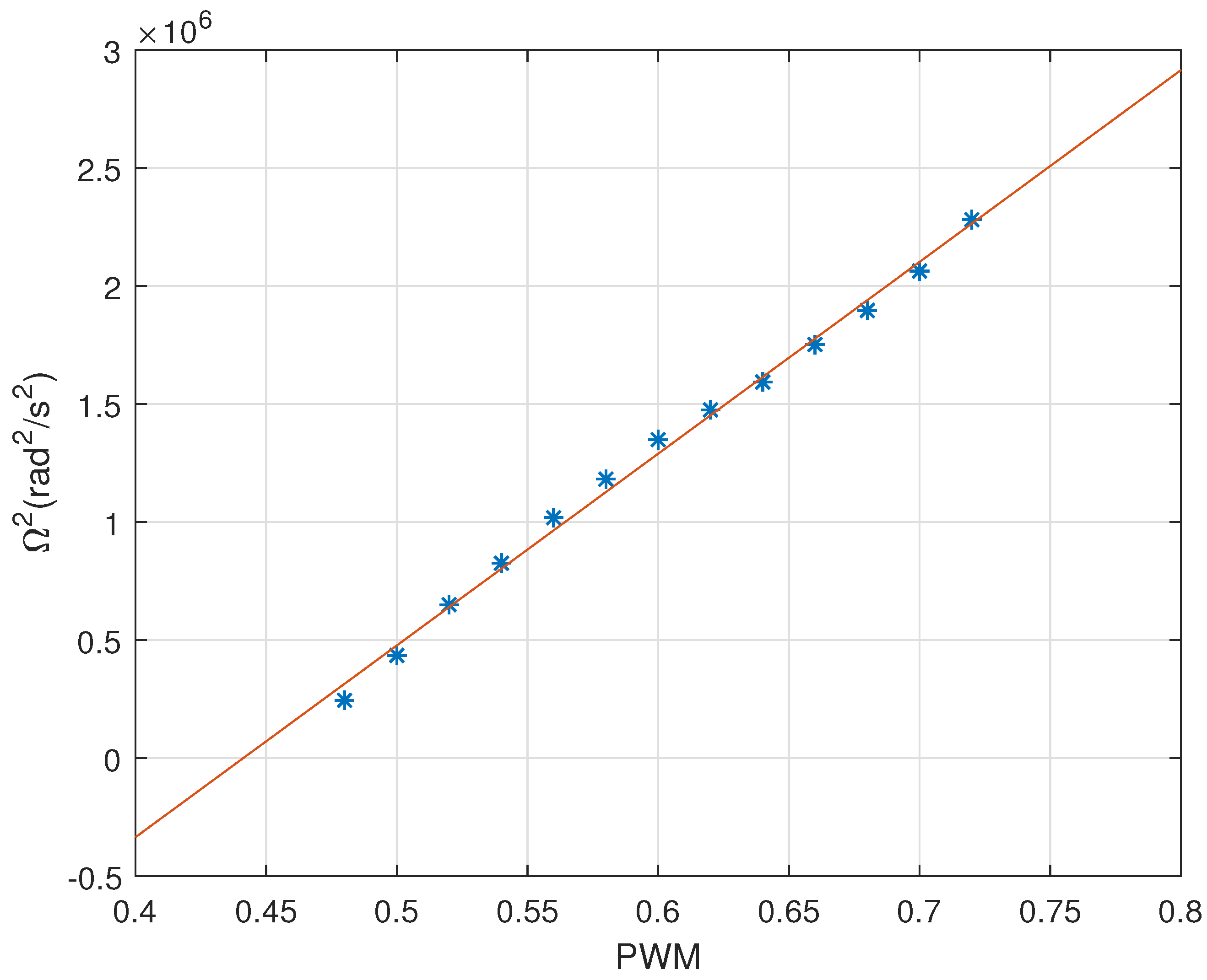
The experimental platform is a custom-built quadrotor based on the QAV-250 frame, featuring an axis-to-axis diagonal length of 250 mm. The airframe utilizes a carbon fiber-reinforced structure to ensure rigidity while minimizing inertia. There are four EMAX MT2204 KV2300 brushless motors paired with 5045 self-tightening propellers. Motor commands are executed via EMAX Simonk 12A electronic speed controllers (ESCs). Attitude feedback is provided by an ICM20602 IMU module, which integrates a 3-axis gyroscope and accelerometer. The ANO-Pioneer flight control board, equipped with an STM32F407VG microcontroller (168 MHz clock speed), runs a real-time operating system to achieve a 200 Hz control loop frequency. This configuration reflects typical small-scale quadrotor dynamics, ensuring the controller’s applicability to similar UAV platforms.

4.1. Parameters

To begin with, some necessary parameters of the quadrotor are measured or estimated. The brushless DC motors are driven by given ESC signals, and the relation between the angular speed of each rotor ${\omega }_i(i=1,2,3,4)$ and PWM $n_i$ signal can be experimentally determined by ${{\omega }_i}^2=k_1{n}_i+k_2$, where $k_1=8.1270\times {10}^6$ and $k_2=-3.5866\times {10}^6$, as shown in Figure 2. For a desired ${\omega }_i$ designed by (5), the ESC signal $n_i$ can be calculated. The rest of the parameters are $l_1=0.077$ m, $l_2=0.102$ m, $I_{xx}=0.0026$ kg·${\mathrm{m}}^2$, $I_{yy}=0.0027$ kg·${\mathrm{m}}^2$, $I_{zz}=0.0047$ kg·${\mathrm{m}}^2$, $k_T=1.468\times {10}^{-6}$ N·${\mathrm{s}}^2$/${\mathrm{rad}}^2$, $k_{\tau }=1.446\times {10}^{-8}$ N·m·${\mathrm{s}}^2$/${\mathrm{rad}}^2$ [29].

The control parameters are the same in subsequent simulations and experiments, which are as follows:

$$\begin{array}{c}{K}_p=\mathrm{diag}\{0.04,0.04,0.01\},K_i=\mathrm{diag}\{0.01,0.01,0.002\},\hfill \\ K_d=\mathrm{diag}\{0.02,0.02,0.005\},K_f=\mathrm{diag}\{0.05,0.05,0.01\},\hfill \\ \sigma =1.5,\gamma =0.02,\rho =0.02,\omega =0.6,\beta =0.75,\epsilon =0.05,\delta ={\displaystyle \frac{1}{9}}\hfill \end{array}$$

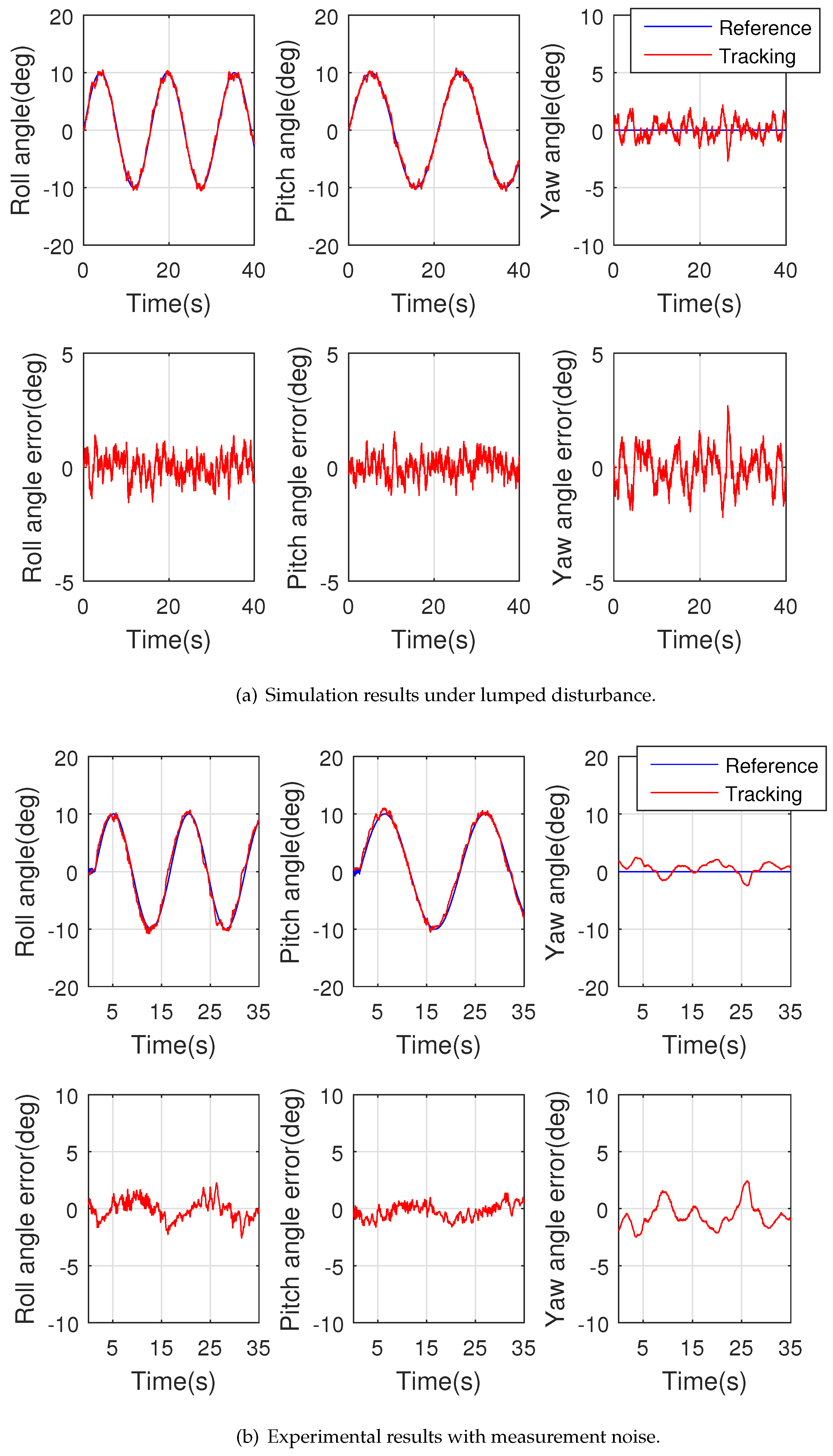
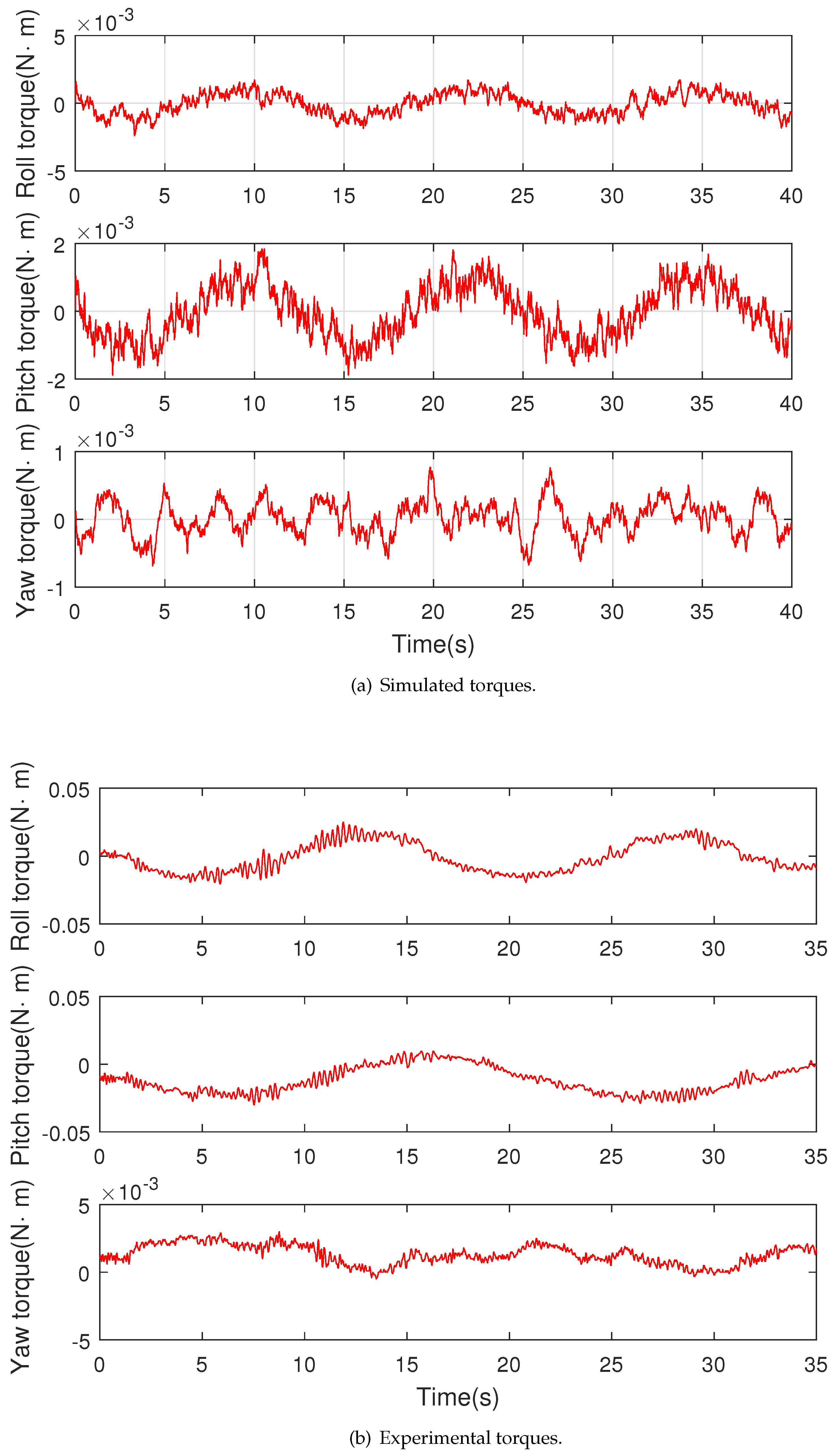
4.2. Simulation Results

In the simulation, the quadrotor attitude tracks a reference attitude command, similar to [24], ${\eta }_d={[10sin\left(0.4t\right)10sin\left(0.3t\right)0]}^T$ and a set of sinusoidal wave disturbances is added as ${\tau }_d=0.001{[sin\left(0.5t\right)sin\left(0.5t\right)0.1sin\left(0.5t\right)]}^T$ N·m. The initial conditions are $\eta \left(0\right)={[0,0,0]}^T$ rad and $\dot{\eta }\left(0\right)={[0,0,0]}^T$ rad/s. The initial values of $z_1$, $z_2$, and $\xi$ are set to zeros. The simulation is carried out in MATLAB 2016a with a sampling time of 5 ms.

By utilizing the ESO, modeling error can also be considered as internal disturbance and can be compensated for. Here, the modeling error is assumed to be mainly caused by inaccurate measurement of moments of inertia, and a bias of $30\%$ is added in simulations. In addition, considering the case in practical application, a measurement noise with zero mean and covariance of 0.01 and a system noise with zero mean and covariance of ${10}^{-6}$ are added in attitude angle and angular acceleration, respectively.

The simulation results are shown in Figure 3a, Figure 4a and Figure 5a. In Figure 3a, it can be observed that the attitude angles can track the reference smoothly in the presence of lumped disturbance and noises. In Figure 4a, the control torques for the roll, pitch, and yaw axes are depicted, generated by the proposed ESO-based nonlinear PID controller. These torques exhibit smooth variations despite the applied lumped disturbance (sinusoidal wave) and measurement/system noises, demonstrating the controller’s ability to stabilize the system. The absence of abrupt spikes indicates effective disturbance rejection through feedforward compensation from the ESO. Figure 5a illustrates the ESO’s estimation performance, where the estimated lumped disturbance (combining external torque, modeling errors, and noise) closely tracks the actual disturbance profile. Minor discrepancies arise due to the $30\%$ inertia bias and added noises in the simulation, yet the bounded estimation errors align with the theoretical convergence guarantees. Together, these figures validate the ESO’s role in actively mitigating disturbances and the controller’s robustness in maintaining precise attitude tracking under noisy conditions.

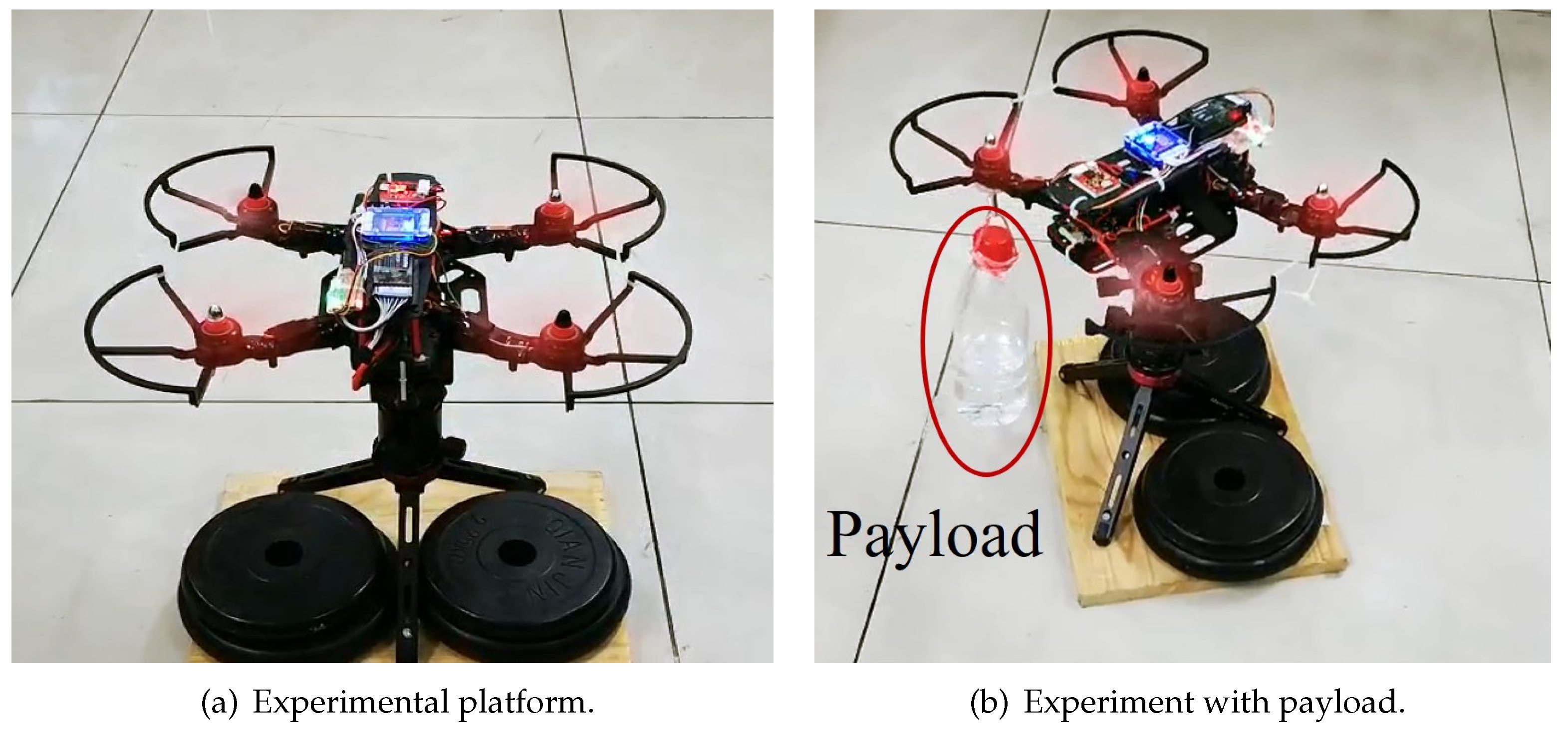
4.3. Experimental Results

In this section, experiments are conducted to illustrate the effectiveness of the proposed method. To this end, an attitude experimental platform is built, as shown in Figure 6a. The quadrotor is fixed to a smooth joint and the translational movement is restricted. The hardware configuration is summarized in the beginning of this section. The attitude control frequency is 200 Hz and the updating frequency of the ESO is 1000 Hz.

4.3.1. Attitude Tracking Control

First, experiments are done to show the attitude tracking performance of the designed controller. The reference trajectory, initial values, and controller gains are set up identically to the simulations. In this case, the experimental results are depicted in Figure 3b, Figure 4b and Figure 5b. The oscillations in attitudes, control torques, and ESO estimations are due to the measurements noise of the IMU and the high-frequency dynamics caused by the vibration of quadrotor. Figure 3b shows the attitude tracking performance, including the reference commands and measurements of roll, pitch, and yaw angles. It was found that the tracking errors are driven into a small neighborhood of the origin, which agrees with the theoretical analysis. To show the efficiency of the ESO, the estimations of the derivatives of attitude tracking errors are also depicted in Figure 5b. The results indicate that the proposed reduced-order ESO can make a relatively accurate estimation even in the presence of measurement noises and high-frequency dynamics.

While experimental results include noise-induced oscillations (Figure 3b), the tracking errors remain bounded within theoretical predictions (Figure 3a). The ESO’s disturbance estimates (Figure 5a vs. Figure 5b) exhibit consistent performance, with experimental deviations attributable to unmodeled high-frequency dynamics, yet still ensure effective compensation.

To quantitatively evaluate the controller’s performance, key metrics such as maximum absolute error (MAE) and root mean square error (RMSE) are computed for both simulation and experimental results. For instance, in Figure 3a, the roll and pitch tracking errors exhibit MAEs of $0.12$ rad and $0.11$ rad, respectively, with RMSEs of $0.08$ rad (roll) and $0.07$ rad (pitch). The yaw channel shows superior precision, achieving an MAE of $0.018$ rad and RMSE of $0.009$ rad under disturbances. Experimental results (Figure 3b) reflect slightly higher but still bounded errors due to real-world noise and vibrations: MAEs of $0.16$ rad (roll), $0.15$ rad (pitch), and $0.025$ rad (yaw), with RMSEs of $0.10$ rad, $0.09$ rad, and $0.015$ rad, respectively. Control torque signals (Figure 4) remain within $\pm 0.25$ N·m (roll/pitch) and $\pm 0.05$ N·m (yaw), demonstrating smooth actuation. The ESO’s disturbance estimation error (Figure 5) maintains an RMSE of $0.003$ N·m in simulations and $0.008$ N·m in experiments, confirming its efficacy despite noise. These quantitative results align with the theoretical UUB guarantees and validate the algorithm’s robustness.

Furthermore, in order to verify that ESO is likely to enhance the robustness of system, another set of experiments will be discussed in Section 4.3.2.

4.3.2. Attitude Stabilization with Disturbance Torque

In this paper, to illustrate the robustness of the proposed method, experiments were carried out in which a payload of 200 g was hung on one arm of the quadrotor at a time instant. It can be approximately considered that a time-varying disturbance torque acts on the quadrotor as the payload swings. The experimental platform is shown in Figure 6b. All the parameters are the same as the previous ones. The results are given in Figure 7, Figure 8 and Figure 9, and the moment that disturbance torque joins is marked in the figures. Figure 7 indicates that there is no abrupt change in attitude angles and the tracking error is still acceptable even subjected to disturbance torque. It can also be observed from Figure 8 and Figure 9 that the disturbance torque can be estimated quickly and compensated for actively in control torques. It is considered that the ESO plays a key role in disturbance rejection, and the proposed method demonstrates a good robustness and tracking accuracy.

5. Conclusions

In this paper, a nonlinear PID controller was investigated for the quadrotor attitude tracking problem. First, the attitude error dynamics were obtained with a lumped disturbance, and a special form of ESO was designed to estimate and compensate for the disturbance. Since the angular velocities were available via IMU, a reduced-order ESO was applied to reduce the phase lag, as well as the influence of measurement noise and high-frequency dynamics. Then, an ESO-based nonlinear PID controller was designed for attitude tracking. Rigorous proof of the convergence of the closed-loop system in the presence of disturbances was provided based on the Lyapunov method. Finally, simulations and experimental results indicate a good tracking accuracy and robustness against disturbance of the proposed method. Despite the proposed method excelling in disturbance rejection and tracking precision, limitations such as manual parameter tuning and actuator saturation warrant further investigation. Therefore, future work will focus on intelligent parameter adaptation (e.g., reinforcement learning) and anti-saturation control of the quadrotor to broaden its applicability.

References

1. Bui, D.N.; Van Nguyen, T.T.; Phung, M.D. Lyapunov-based nonlinear model predictive control for attitude trajectory tracking of unmanned aerial vehicles. Int. J. Aeronaut. Space Sci. 2023, 24, 502–513. [Google Scholar] [CrossRef]
2. Lopez-Sanchez, I.; Pérez-Alcocer, R.; Moreno-Valenzuela, J. Trajectory tracking double two-loop adaptive neural network control for a Quadrotor. J. Frankl. Inst. 2023, 360, 3770–3799. [Google Scholar] [CrossRef]
3. Lopez-Sanchez, I.; Moyrón, J.; Moreno-Valenzuela, J. Adaptive neural network-based trajectory tracking outer loop control for a quadrotor. Aerosp. Sci. Technol. 2022, 129, 107847. [Google Scholar] [CrossRef]
4. Lopez-Sanchez, I.; Moreno-Valenzuela, J. PID control of quadrotor UAVs: A survey. Annu. Rev. Control 2023, 56, 100900. [Google Scholar] [CrossRef]
5. Hong, K. Simulation and analysis of stability of UAV control system based on PID control under different wind forces. J. Phys. Conf. Ser. 2023, 2649, 012011. [Google Scholar] [CrossRef]
6. Ghanifar, M.; Kamzan, M.; Tayefi, M. Different Intelligent Methods for Coefficient Tuning of Quadrotor Feedback-linearization Controller. J. Aerosp. Sci. Technol. 2023, 16, 56–65. [Google Scholar]
7. Najm, A.A.; Ibraheem, I.K. Nonlinear PID controller design for a 6-DOF UAV quadrotor system. Eng. Sci. Technol. Int. J. 2019, 22, 1087–1097. [Google Scholar] [CrossRef]
8. Jin, G.G.; Pal, P.; Chung, Y.K.; Kang, H.K.; Yetayew, T.T.; Bhakta, S. Modelling, control and development of GUI-based simulator for a quadcopter using nonlinear PID control. Aust. J. Electr. Electron. Eng. 2023, 20, 387–399. [Google Scholar] [CrossRef]
9. Wang, S.; Polyakov, A.; Zheng, G. Quadrotor stabilization under time and space constraints using implicit PID controller. J. Frankl. Inst. 2022, 359, 1505–1530. [Google Scholar] [CrossRef]
10. Najm, A.A.; Azar, A.T.; Ibraheem, I.K.; Humaidi, A.J. A Nonlinear PID Controller Design for 6-DOF Unmanned Aerial Vehicles; Academic Press: Cambridge, MA, USA, 2021; pp. 315–343. [Google Scholar]
11. Moreno-Valenzuela, J.; Pérez-Alcocer, R.; Guerrero-Medina, M.; Dzul, A. Nonlinear PID-type controller for quadrotor trajectory tracking. IEEE/ASME Trans. Mechatron. 2018, 23, 2436–2447. [Google Scholar] [CrossRef]
12. Zhu, B.; Huo, W. Nonlinear control for a model-scaled helicopter with constraints on rotor thrust and fuselage attitude. Acta Autom. Sin. 2014, 40, 2654–2664. [Google Scholar] [CrossRef]
13. Jeong, H.; Suk, J.; Kim, S. Control of quadrotor UAV using variable disturbance observer-based strategy. Control Eng. Pract. 2024, 150, 105990. [Google Scholar] [CrossRef]
14. Li, C.; Wang, Y.; Yang, X. Adaptive fuzzy control of a quadrotor using disturbance observer. Aerosp. Sci. Technol. 2022, 128, 107784. [Google Scholar] [CrossRef]
15. Gong, W.; Li, B.; Ahn, C.K.; Yang, Y. Prescribed-time extended state observer and prescribed performance control of quadrotor UAVs against actuator faults. Aerosp. Sci. Technol. 2023, 138, 108322. [Google Scholar] [CrossRef]
16. Zhao, K.; Zhang, J.; Shu, P.; Dong, X. Composite Nonlinear Extended State Observer-Based Trajectory Tracking Control for Quadrotor Under Input Constraints. IEEE Trans. Circuits Syst. I Regul. Pap. 2023, 70, 4126–4136. [Google Scholar] [CrossRef]
17. Guo, B.; Zhao, Z. On the convergence of an extended state observer for nonlinear systems with uncertainty. Syst. Control Lett. 2011, 60, 420–430. [Google Scholar] [CrossRef]
18. Wang, L.; Pei, H. Geometric prescribed-time control of quadrotors with adaptive extended state observers. Int. J. Robust Nonlinear Control 2024, 34, 7460–7479. [Google Scholar] [CrossRef]
19. Li, J.; Cao, C.; Xu, J. An extended state observer-based active disturbance rejection control for quadrotor attitude stabilization. Mechatronics 2022, 85, 102853. [Google Scholar]
20. Luo, Y.; Ma, J.; Hu, J. Fault-tolerant tracking control for quadrotor UAV with actuator saturation and multiple uncertainties. ISA Trans. 2023, 134, 373–385. [Google Scholar]
21. Zhang, Y.; Ding, S.; Li, Y. Data-driven fault-tolerant tracking control for quadrotor UAV with actuator failure and external disturbance. IEEE Trans. Ind. Electron. 2023, 70, 5962–5972. [Google Scholar]
22. Zhao, S.; Li, H.; Wang, L. Active disturbance rejection flight control for quadrotors based on nonlinear extended state observer. Aerospace 2023, 10, 327. [Google Scholar]
23. Zhou, Y.; Liu, Z.; Zhang, C. Anti-saturation prescribed-time trajectory tracking control of quadrotors with nonlinear observers. IEEE Trans. Control Syst. Technol. 2024; early access. [Google Scholar]
24. Ma, D.; Xia, Y.; Shen, G.; Jiang, H.; Hao, C. Practical fixed-time disturbance rejection control for quadrotor attitude tracking. IEEE Trans. Ind. Electron. 2020, 68, 7274–7283. [Google Scholar] [CrossRef]
25. Chen, H.; Du, L.; Zhang, X. A robust disturbance observer-based control approach for quadrotors in uncertain environments. IEEE Access 2022, 10, 59338–59350. [Google Scholar]
26. Tang, H.; Yu, M.; Zhang, J. Reduced-order disturbance observer-based trajectory tracking control for quadrotors under bounded uncertainties. Robot. Auton. Syst. 2023, 164, 104383. [Google Scholar]
27. Yan, S.; Liu, Q.; Zhang, L. Robust trajectory tracking control of quadrotors under lumped disturbances: Simulation and experiments. Aerosp. Sci. Technol. 2022, 124, 107520. [Google Scholar]
28. Raffo, G.V.; Ortega, M.G.; Rubio, F.R. An integral predictive/nonlinear H control structure for a quadrotor helicopter. Automatica 2010, 46, 29–39. [Google Scholar] [CrossRef]
29. Shi, D.; Dai, X.; Zhang, X.; Quan, Q. A Practical Performance Evaluation Method for Electric Multicopters. IEEE/ASME Trans. Mechatron. 2017, 22, 1337–1348. [Google Scholar] [CrossRef]
Figure 1. Body-fixed frame and earth-fixed frame for the quadrotor.
Processes 13 01470 g001
Figure 2. Relationship between ESC signal and the angular speed of rotor.
Processes 13 01470 g002
Figure 3. Attitude tracking performance and errors.
Processes 13 01470 g003
Figure 4. Control torques of roll, pitch, and yaw axes.
Processes 13 01470 g004
Figure 5. Disturbance estimations of proposed ESO.
Processes 13 01470 g005
Figure 6. Quadrotor attitude experimental platform.
Processes 13 01470 g006
Figure 7. Experimental results: attitude tracking performance with payload disturbance.
Processes 13 01470 g007
Figure 8. Experimental results: control torques for roll, pitch, and yaw angles in payload disturbance scenario.
Processes 13 01470 g008
Figure 9. Experimental results: estimation performance of the proposed ESO in payload disturbance scenario.
Processes 13 01470 g009
Disclaimer/Publisher’s Note: The statements, opinions and data contained in all publications are solely those of the individual author(s) and contributor(s) and not of MDPI and/or the editor(s). MDPI and/or the editor(s) disclaim responsibility for any injury to people or property resulting from any ideas, methods, instructions or products referred to in the content.