Mitigating Partial Shading Effects in Photovoltaic Systems Using Particle Swarm Optimization-Tuned Sliding Mode Control

Abstract

The power output of a photovoltaic (PV) system is inherently dependent on climatic factors. To maximize the energy harvested from PV arrays, maximum power point tracking (MPPT) algorithms are employed. These algorithms dynamically adjust the operating point of the system to extract the maximum available power. However, under partial shading conditions (PSCs), conventional MPPT algorithms often fail to locate the global maximum power point, leading to suboptimal power extraction. In this study, a robust MPPT technique based on sliding mode control (SMC) is proposed to enhance tracking efficiency and optimize power extraction from PV arrays under PSC. Particle swarm optimization (PSO) is incorporated into the MPPT framework, enabling the dynamic tuning of SMC parameters for improved adaptability and performance. The proposed SMC structure is designed to regulate the duty cycle of a boost converter, ensuring effective power conversion. The system is simulated in Matlab/Simulink for various PSCs. The simulation results demonstrate that the PSO-tuned SMC methodology exhibits superior tracking performance, enabling the PV system to rapidly and accurately converge to the true MPP under varying weather and shading scenarios. The findings indicate that the proposed technique enhances the efficiency and reliability of PV energy harvesting in PSCs.

1. Introduction

The energy crisis and environmental pollution have made new forms of green energy more popular, as they have less environmental impact and are important tools in the fight against global warming—a fight which was started by the Paris Agreement at the 2015 United Nations Climate Change Conference [1]. Solar energy is the most common type of green energy due to its advantages, such as not polluting the environment, being widespread, freely available, easy to use, and requiring low maintenance [2]. A photovoltaic (PV) electrical energy production system is the most common system for generating energy from solar energy. The required voltage and power values are obtained from the PV array, which is formed by connecting PV modules in series and parallel. A power electronic converter is then used to supply the loads with appropriate voltage and power values.

Climatic and environmental conditions, such as solar irradiation, temperature, and dust, affect the efficiency of the PV system. Today, the efficiency of PV panels is still limited to about 15–25% [3]. The efficiency of a PV array can be improved by maintaining the PV to work at the maximum power point (MPP). Popular methods of maximum power point tracking (MPPT) are perturb and observe [4], hill climbing [5], and incremental conductance [6]. These conventional MPPT techniques can be used with higher efficiency for accurate tracking of the MPP under uniform solar irradiation, where the power–voltage (P-V) characteristic curve of the PV array has only one maximum point. These conventional MPPT techniques present poor performance in quickly changing environmental conditions [7]. Due to environmental conditions, as well as the presence of clouds, trees, and dust on the PV array, the P-V curve has more than one maximum point. In this condition, the different cells receive different irradiation values, which is known as partial shading. The MPP methods that utilize fractional open-circuit voltage [8] and short circuit current for MPP tracking, by assuming a linear relationship between PV array voltage and current, respectively, fail under partial shading conditions (PSCs) due to loss of proportionality.

Multiple MPPs occur in the PV systems operating under PSCs. These MPPs are local maximum power points (LMPPs) and one global maximum power point (GMPP). The system should work at the GMPP in order to obtain maximum efficiency from the panels.

Using conventional MPP techniques in this PSC can result in tracking LMPPs instead of the GMPP on the P-V characteristic curve of the PV array. This situation reduces the system efficiency and the electrical energy converted from solar energy. Therefore, different MPPT algorithms are introduced for the partially shaded and irradiance change conditions to track the MPP instead of LMPPs and to force the system to operate at higher efficiency [9]. Besides the combinations of different optimization techniques, such as particle swarm optimization (PSO) [10], bee colony, and differential evolution, with the conventional MPPT algorithms, machine learning [11] and artificial intelligence techniques, such as neural networks [12], fuzzy logic [13], and sliding mode control (SMC), are the most commonly used for the tracking of MPP under PSCs.

The PSO technique is the most commonly used method of MPPT for PV systems under PSCs [14,15]. Although the algorithm has good performance in the PSC, the output power oscillates, and it is initial-condition-dependent and may fail in some conditions [16].

Irrespective of the ability to operate on a non-linear characteristic curve, the neural network requires comprehensive computation. The network should be intensively trained [17].

The fuzzy logic method for the MPPT has the advantage of good tracking under changing climatic conditions, but the system becomes complex, causing reduced response speed [18].

SMC [19] is a non-linear control technique. Due to its fast dynamic response, reliability, and robustness, it is used for controlling switching converters [20] in PV power-producing systems.

The intelligent MPPT techniques have better performance in quickly changing environmental conditions [21].

Intelligent techniques can accurately track the GMPP, being independent of shading, the P-V characteristic curve, and the pattern of the PV array. However, the complexity in implementation and the initial point selection for the convergence are the disadvantages of the system. Taking many samples at different points on the array P-V characteristic curve to find the GMPP reduces the speed of tracking.

Most of the intelligent techniques used for MPPT produce stable and accurate tracking under stable conditions, but their stability and accuracy are reduced in rapidly changing environmental or loading conditions. A suitable MPPT method that can be used in changing environmental conditions can be selected based on performance parameters such as complexity, convergence rate, speed, sensor requirement, robustness, and reliability.

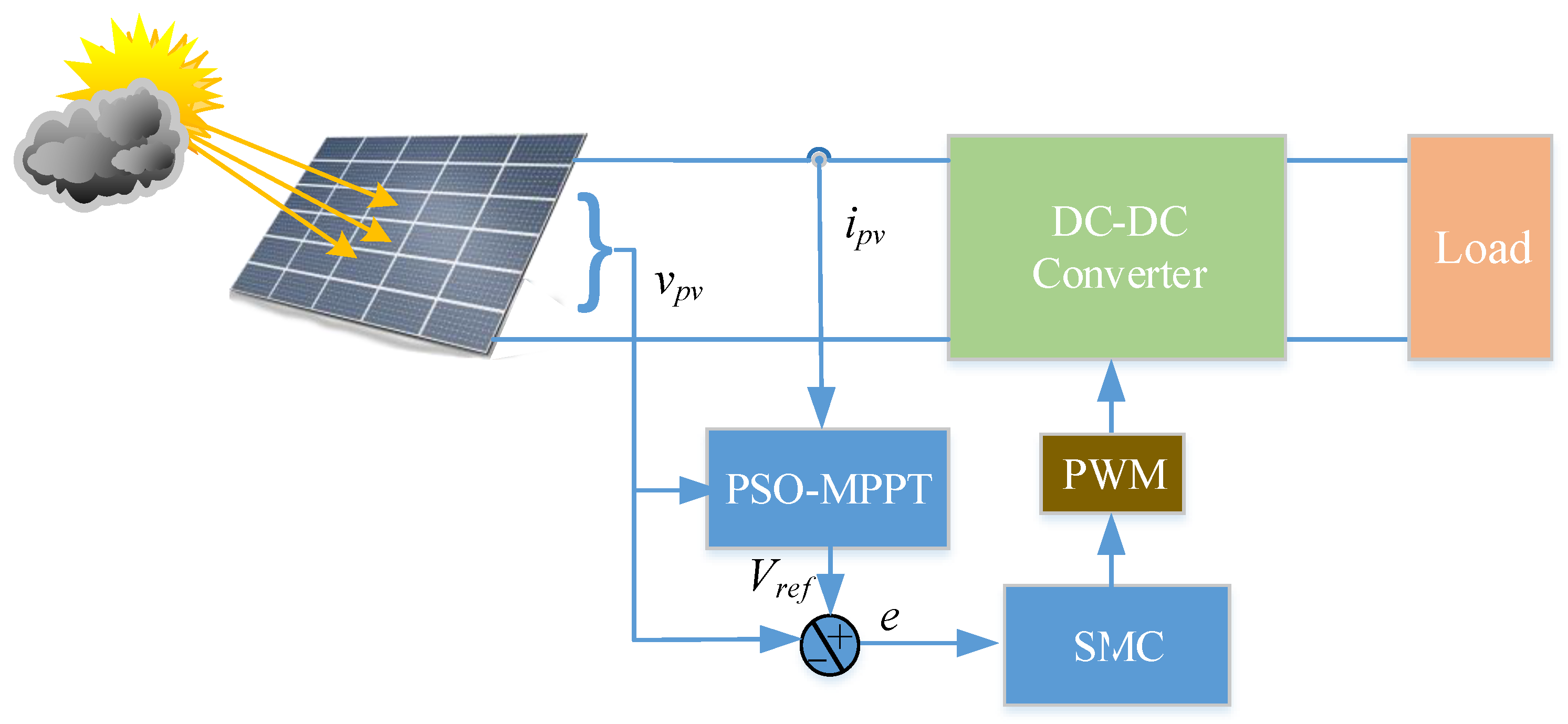
In this paper, due to the characteristics of compact structure, reliability, and robustness to un-modeled dynamics and input changes, the SMC technique is used as the MPPT controller to obtain maximum power from a PV array under PSCs. PSO is combined to tune the parameters of SMC to obtain significant benefits such as enhanced performance, faster convergence, and ease of implementation.

The PSO-tuned SMC-based MPPT algorithm offers several benefits over traditional MPPT techniques such as providing robustness against uncertainties and disturbances, ensuring reliable operation in PSCs, fast tracking, and accurate convergence to the MPP, resulting in increased energy harvesting and improved system efficiency.

The main contribution of this study is the development of a sliding mode controller aimed at mitigating power quality issues in the grid while ensuring a stable DC voltage output. The PSO algorithm is employed to optimize the controller parameters based on the derived design equations. The used control algorithm forces the system to operate at the MPP with higher efficiency. The performance of the PV power is examined under different environmental conditions such as insulation, temperature, and PSCs.

The proposed PSO-tuned SMC-based MPPT technique differs from existing hybrid MPPT methods in several key aspects:

While prior studies have combined optimization algorithms with sliding mode control, most of these approaches either use optimization purely for offline parameter tuning or apply it intermittently during operation, resulting in limited adaptability to highly dynamic partial shading conditions (PSCs). In contrast, our method integrates PSO dynamically within the MPPT loop to continuously adjust the critical parameters of the sliding mode controller in real time. This dynamic tuning enhances the system’s adaptability to rapidly changing environmental conditions.

Additionally, conventional hybrid methods often treat the optimization algorithm and the SMC separately, leading to increased system complexity and potential instability. Our approach designs the PSO and SMC in a tightly coupled framework, where the PSO directly influences the sliding surface parameters and switching gain, ensuring that the controller remains robust while avoiding excessive chattering.

The proposed method focuses on minimizing convergence time to the global maximum power point (GMPP) without sacrificing steady-state accuracy, even under severe PSCs. Simulation results presented in the study show a significant improvement in both tracking speed and power extraction efficiency.

It is aimed here to have a reliable control that tracks the MPP in both uniform and changing climatic conditions and force the system to harvest maximum power.

2. PV Array in Partial Shading Conditions

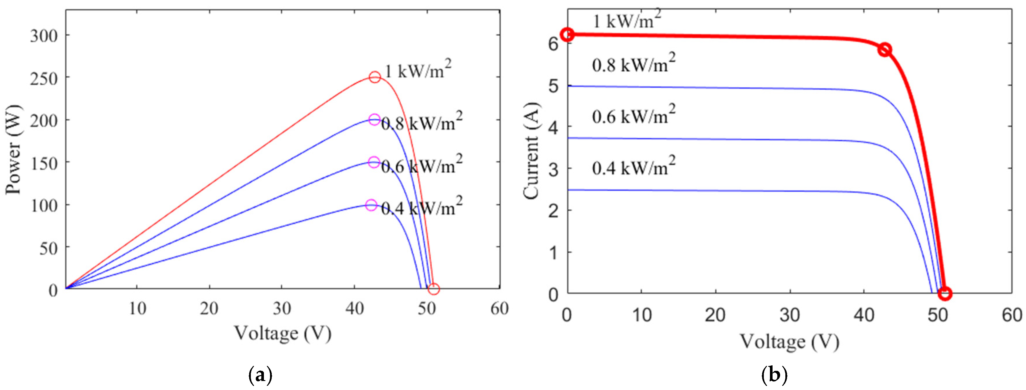
PV modules are affected by solar radiation and temperature and exhibit different characteristic curves under uniform solar illumination and PSCs. Figure 1 shows the P-V and I-V characteristic curves of the PV module under uniform irradiations of 400 W/m², 600 W/m², 800 W/m², and 1000 W/m² at 25 °C.

PV arrays are generally installed on rooftops and in inclined areas with higher northern and lower southern orientations. Environmental factors such as surrounding buildings, trees, and clouds, as in Figure 2, cause one or more solar panels to be completely or partially shaded. In this case, the efficiency of the shaded panels decreases and the overall power generation in the system is reduced.

PV power-producing systems are formed by several PV cells connected in series to increase the voltage produced or parallel to increase the total current drawn. The normal operation of a PV system occurs when all the panels in the system experience the same solar conditions as they are part of a common solar array. However, blocking of sunlight onto the cell or panel by leaves, trees, buildings, or antennas causes some of the cells to experience different solar conditions which leads to mismatches between cells or panels.

When some cells of the panel are shaded, the series connected cells become reverse biased. The current cannot flow around the shaded cells. Excess power dissipation occurs in the shaded cell, which overheats the shaded area, increases the temperature, and causes hotspot formation. Consequently, a reduction in the output power of the module is observed [22]. In PSCs, the shaded PV cell behaves as a load and affects the efficiency, reliability, and safety of the system.

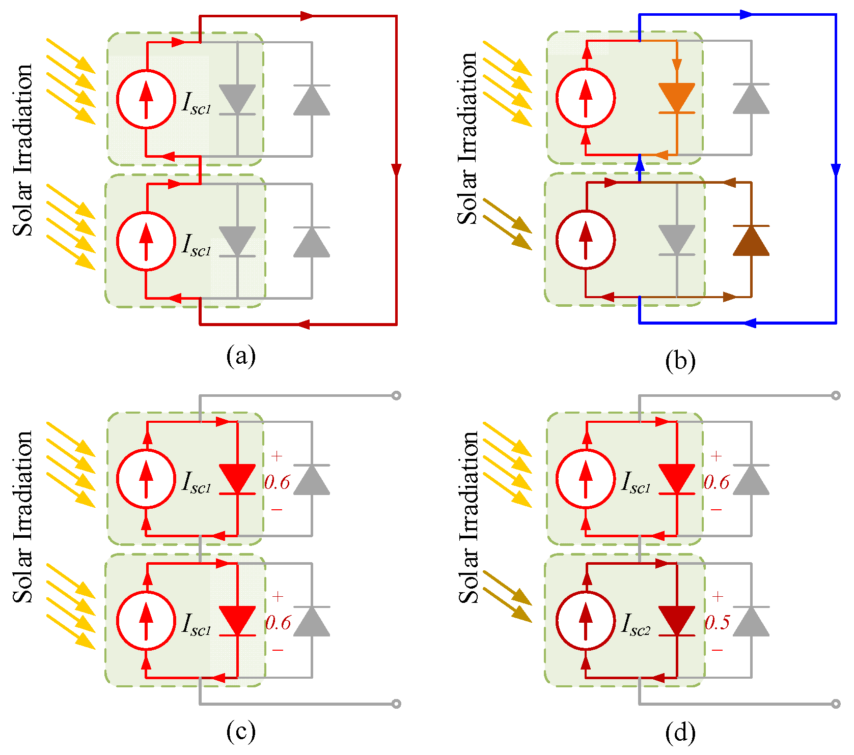
A by-pass diode is connected in parallel with opposite polarity to the PV modules to avoid this problem. The effect of the by-pass diode on the operation of the solar cell, in both short circuit and open circuit conditions, is presented in Figure 3.

In Figure 3, the circuit elements inside the dotted line are the equivalent of a solar cell. The current source is a light-dependent source. The diodes outside the dotted line are by-pass diodes. In normal operation conditions all the solar cells are forward biased and therefore the by-pass diodes are reverse biased and non-conducting. If a cell is reverse biased because of mismatched short circuit current between serial connected cells, then the by-pass diode conducts and lets the current from unshaded cells flow through the by-pass diode of the shaded cell. The reverse bias voltage of the shaded cell is reduced which limits the current and prevents hotspot heating.

In Figure 3a both of the solar cells experience the same solar conditions. In short circuit conditions, the same current passes through the cells and the voltages across the cell and by-pass diodes are zero. Hence, the by-pass diode is non-conducting and has no effect on the circuit. In Figure 3b the solar cell at the bottom is shaded and receives less solar illumination than the upper solar cell. In this case, in the short circuit condition different amounts of current flow through the solar cells. Some of the current of the upper solar cell, that receives full solar illumination, forward biases the cell junction. This voltage then forward biases the shaded cell by-pass diode, resulting in the current passing through it. The by-pass diode of the upper cell is reverse biased and has no effect. The shaded cell is reverse biased.

Figure 3c shows the case when both cells operate under the same solar values in open circuit conditions. The same current I_sc flows through both of the cells and forward biases the cells. The by-pass diodes are reverse biased and non-conducting and have no effect on the operation. In Figure 3d the cells are operating in open circuit conditions but the bottom cell is shaded. Different current flows through each cell. The open circuit voltage of the shaded cell is reduced. The by-pass diodes are reverse biased and remain non-conductive.

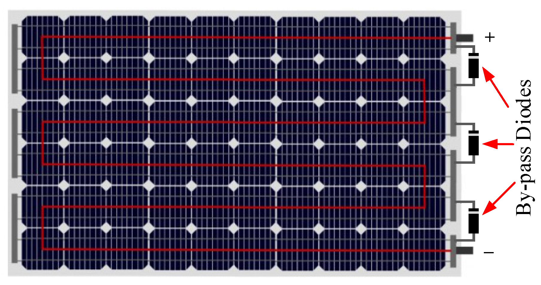
In practice, as shown in Figure 4, by-pass diodes are parallel connected to group of cells instead of each cell or PV modules for economic reasons. In Figure 4, by-pass diodes are connected in parallel to every set of 10 cells to form path for the current under PSCs. Under uniform irradiance, each by-pass diode is reverse biased. When partial shading occurs the PV module becomes reverse biased by other PV modules causing by-pass conduction. Thus, the by-pass diodes short circuit the shaded PV modules. The array voltage drops by an amount corresponding to the sum of the by-passed cell voltages and the diode forward voltage, but current through the unshaded cells continues to flow. The current flows through the by-pass diodes, hence the power loss due to shaded PV modules is reduced.

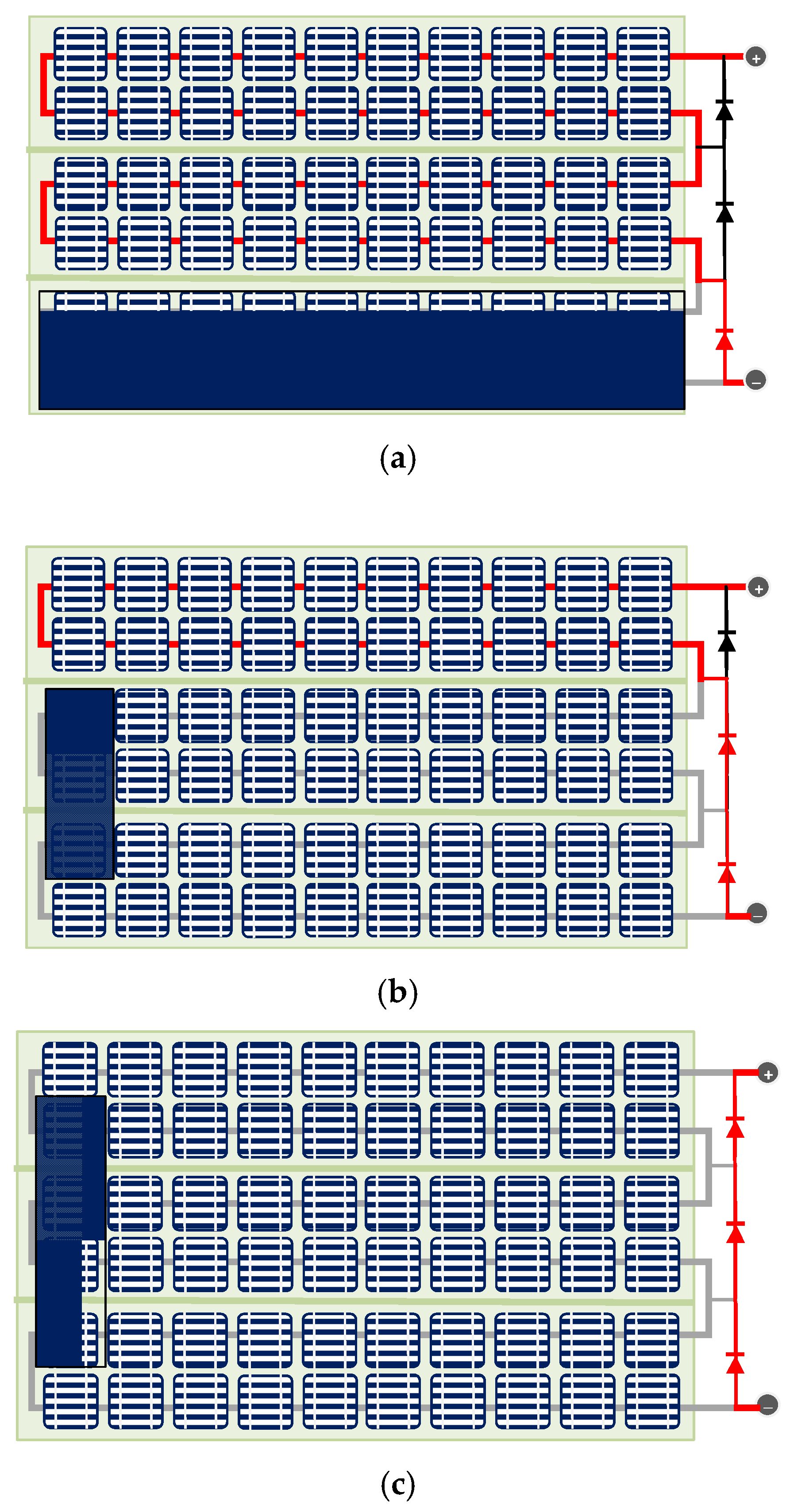
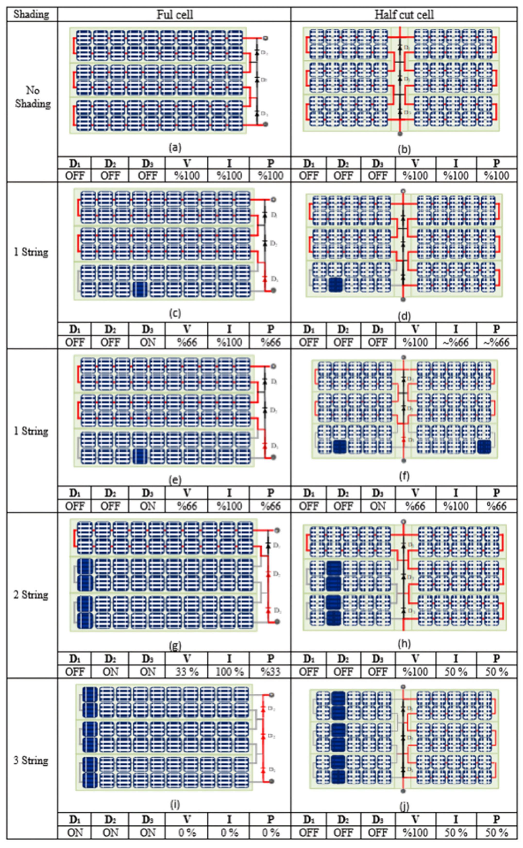
As seen in Figure 5, the effect of the shading depends on the position of the shading on the string. A small amount of shading can be more effective than a larger area as it causes more by-pass diodes to conduct.

In Figure 5a 20 cells are affected by shading. The by-pass diode in the shaded string turns on and 1/3 of the string is by-passed by the diode. The panel continues to produce 2/3 of its total power. In Figure 5b, three cells are shaded. Two strings are by-passed by the diodes, and only one string produces power. The system produces only 1/3 of its total power, 2/3 power loss occurs. However, in Figure 5c only four cells are affected by shading. Since all three by-pass diodes are conducting, the panel produces no power at all.

One way to reduce the shading effect of the PV panels is to use half-cut cells. Cutting cells in half halves the current flowing through each cell. Thus, resistive losses are reduced, resulting in better performance.

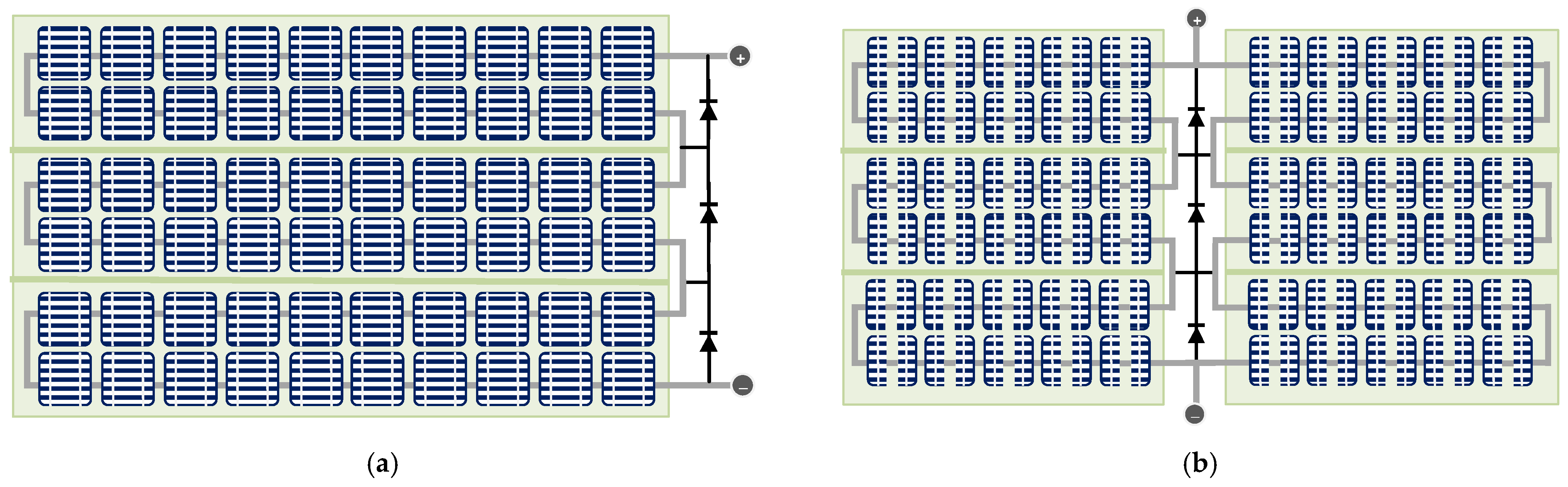
Using half-cut solar cells increases the energy output by reducing the size of the cell, thus more cells are placed on a panel. The panel is split into two parts, which operate independently of each other. Thus, more power is generated when one part is shaded. Figure 6a shows a three-string series wired PV panel constructed with full cells. However, Figure 6b represents the PV panel constructed with half-cut cells. As seen, the panel is split in half, having a six-cell group instead of three as in the full cell structure. The by-pass diodes are connected across both sides of the panel.

When a cell in a row of the PV panel with full cells is shaded, the entire series connected row fails to generate energy. This renders one-third of the panel inactive in terms of energy production.

In the case of the half-cut cell structure, if a cell in a row of a string at the left side is shaded, the cells in that row cannot produce energy. The other rows both on the left and right continue to produce energy. As seen in Figure 7, more energy is produced when comparing the full cell structure because only 1/6 of the panel is not producing energy instead of 1/3. This is because a half-cut cell has two MPPs in its power characteristic curve which are LMPP and GMPP. The local maximum is due to the lower current while maintaining normal voltage in the unshaded half rather than activating the by-pass diode. This condition is represented in Figure 7d. The other shading scenarios are represented in Figure 7.

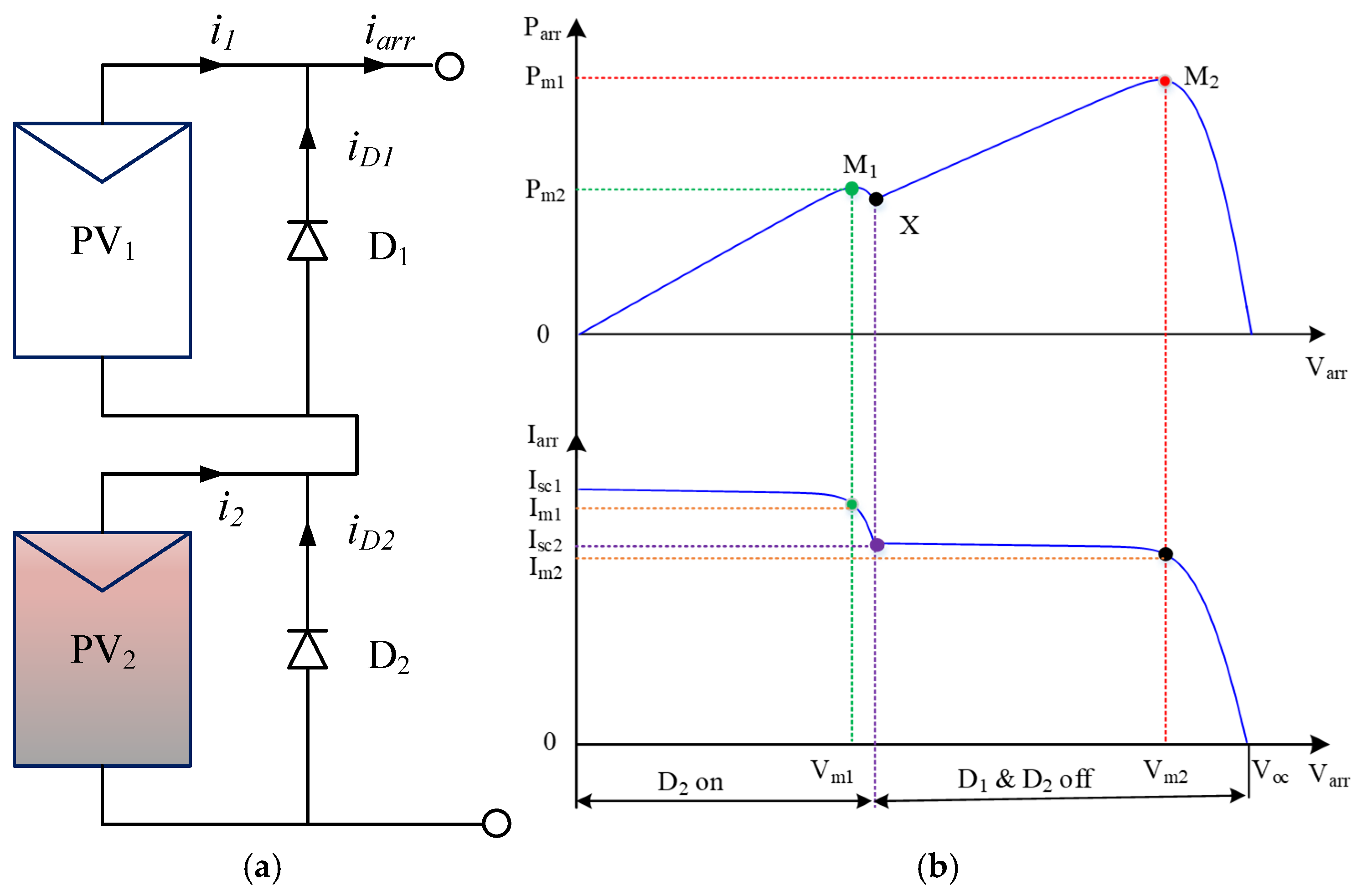
When by-pass diodes are connected in parallel to the PV modules, in the case of PS, the current flows through the by-pass diode instead of the shaded PV module. In this case multiple steps in the I-V characteristic curve and multiple peaks in the P-V characteristic curve occur.

Figure 8a shows the PV array with two modules, PV₁ and PV₂. If PV₁ receives more illumination than PV₂, then the current and voltage of PV₁ become higher than those of PV₂ [23].

When the array current, i_arr, is smaller than the current of PV₂, i₂, both PV₁ and PV₂ generate energy, and the array voltage becomes the sum of the voltages of PV₁ and PV₂.

When the array current i_arr exceeds i₂, diode D₂ becomes forward biased and starts to conduct, and thus PV₂ is by-passed and does not produce energy. Then, the output voltage of the array is equal to that of PV₁. As shown in Figure 8b, the I–V curve of the PV array has two stairs, and the P–V curve of the PV array has two peak PPs, M₁ and M₂. Point X is the transition point.

In the interval at the left of point X, only PV₁ operates, and the PP-current is I_m1 and the peak PP-voltage is V_m1, the details can be found in [24].

In the interval at the right of the transition point X, PV₁ and PV₂ operate together. Because PV₁ produces nearly constant voltage and the turning point of the I–V curve is mainly affected by PV₂, the peak PP-current is I_m2, and the peak PP-voltage is V_m2. V_oc1 is approximately equal to V_oc2, which is equal to half of the OC-voltage of the PV array, V_oc. The complete relationship of PV array voltage and current between irradiance and temperature can be found in [25].

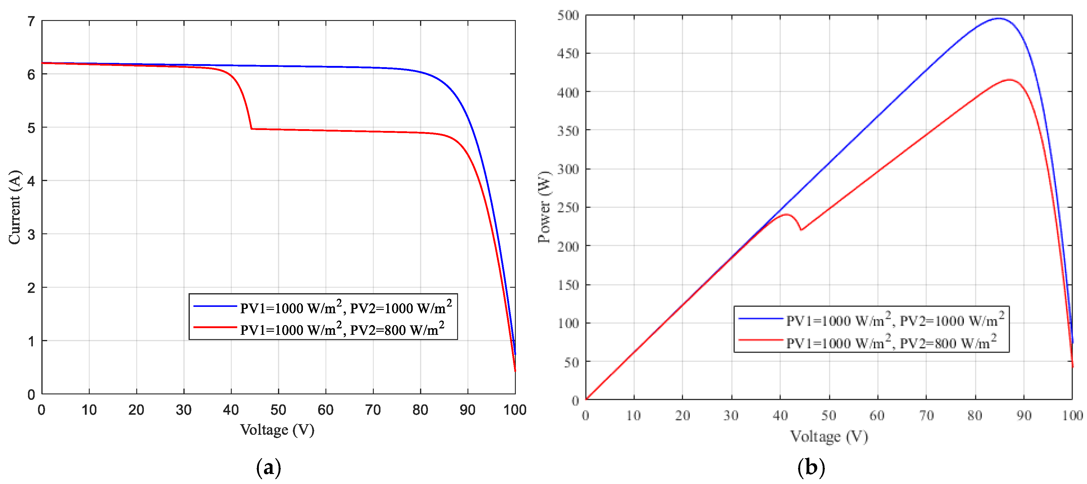
P-V and I-V characteristics of two series connected PV modules, whose parameters are given in

Table 1. Parameters of PV Module.

Parameter	Values
Module	SunPower SPR-X20-250-BLK
Maximum power (W)	249.952
Cells per module (Ncell)	72
Open circuit voltage Voc (V)	50.93
Short circuit current Isc (A)	6.2
Voltage at maximum power point Vmp (V)	42.8
Current at maximum power point Imp (V)	5.84

, under uniform and non-uniform irradiation values are shown in Figure 9. These figures are obtained by simulation of Figure 8a.

The blue line represents the case when both PV₁ and PV₂ have the same solar illumination values of 1000 W/m². The red line shows the case when PV₁ has 1000 W/m² solar illumination but PV₂ receives 800 W/m² solar illumination.

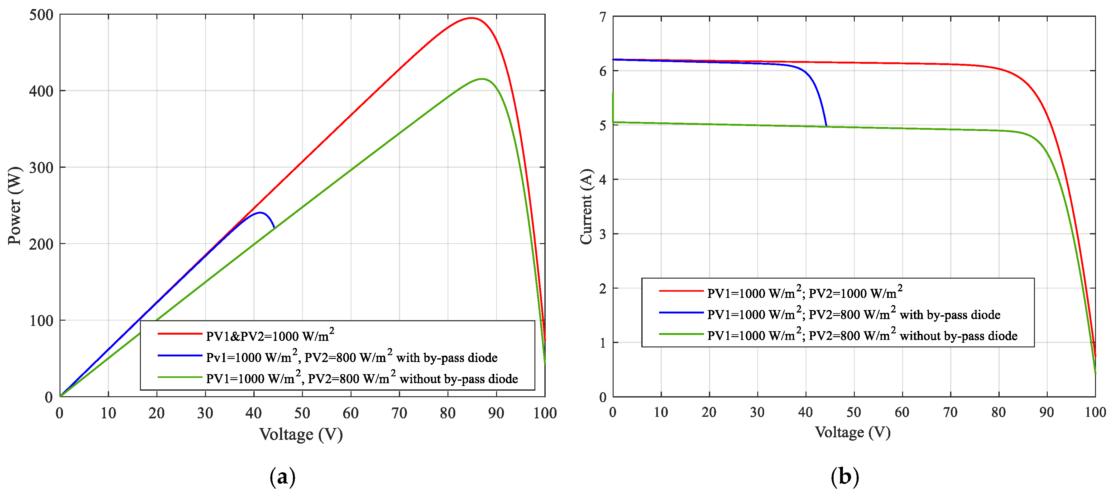
Figure 10a shows P-V characteristic curves and Figure 10b shows I–V characteristic curves of a series connected two-PV-array system, both with and without by-pass diodes, under identical and varying irradiation conditions. The red line represents the case where both PV₁ and PV₂ receive the same solar irradiance of 1000 W/m². The green line shows the case where PV₁ receives 1000 W/m² and PV₂ receives 800 W/m² with no by-pass diodes connected. The blue line shows the same irradiation condition but with by-pass diodes connected.

Similarly, for n PV modules connected in series under PSCs, the I–V curve will contain n steps, and the P–V curve will consist of n intervals, each having one peak PP. Thus, the P–V curve has n peak PPs.

The output power and voltage of a single PV module are limited and must be combined in series and parallel to achieve the required power and voltage levels in a PV system.

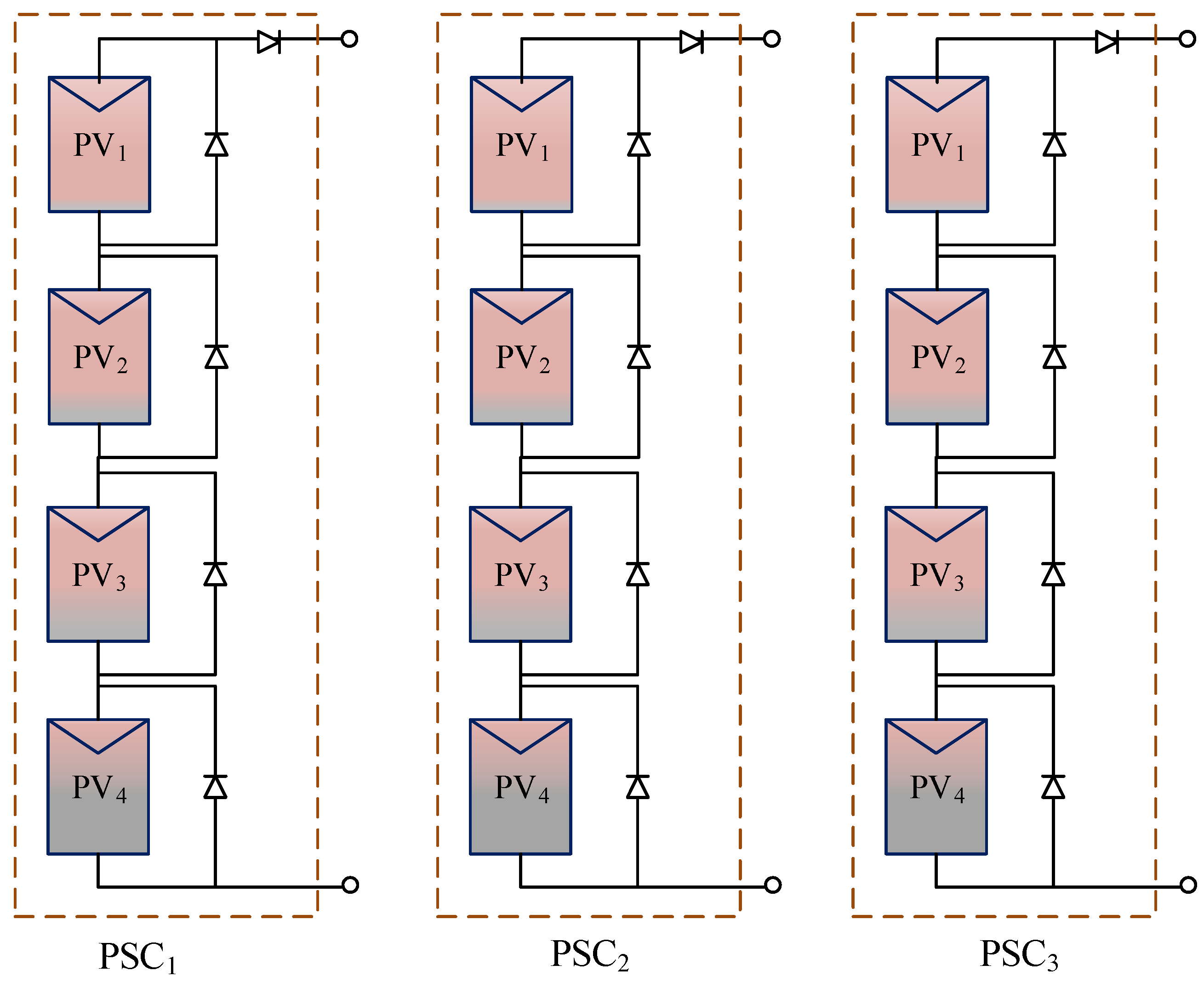
When a PV array is partially shaded, its output characteristics differ from those of a single PV module. Figure 11 shows the partially shaded PV array topology. In this system, four PV modules are connected in series. Different shading values are applied in PSC₁, PSC₂, and PSC₃ scenarios, in which each PV receives different irradiation values, as listed in

Table 2. Various PSCs.

Irradiation (W/m2)
	PV1	PV2	PV3	PV4
PSC1	1000	800	600	400
PSC2	900	700	500	300
PSC3	600	400	200	100

, under the same temperature.

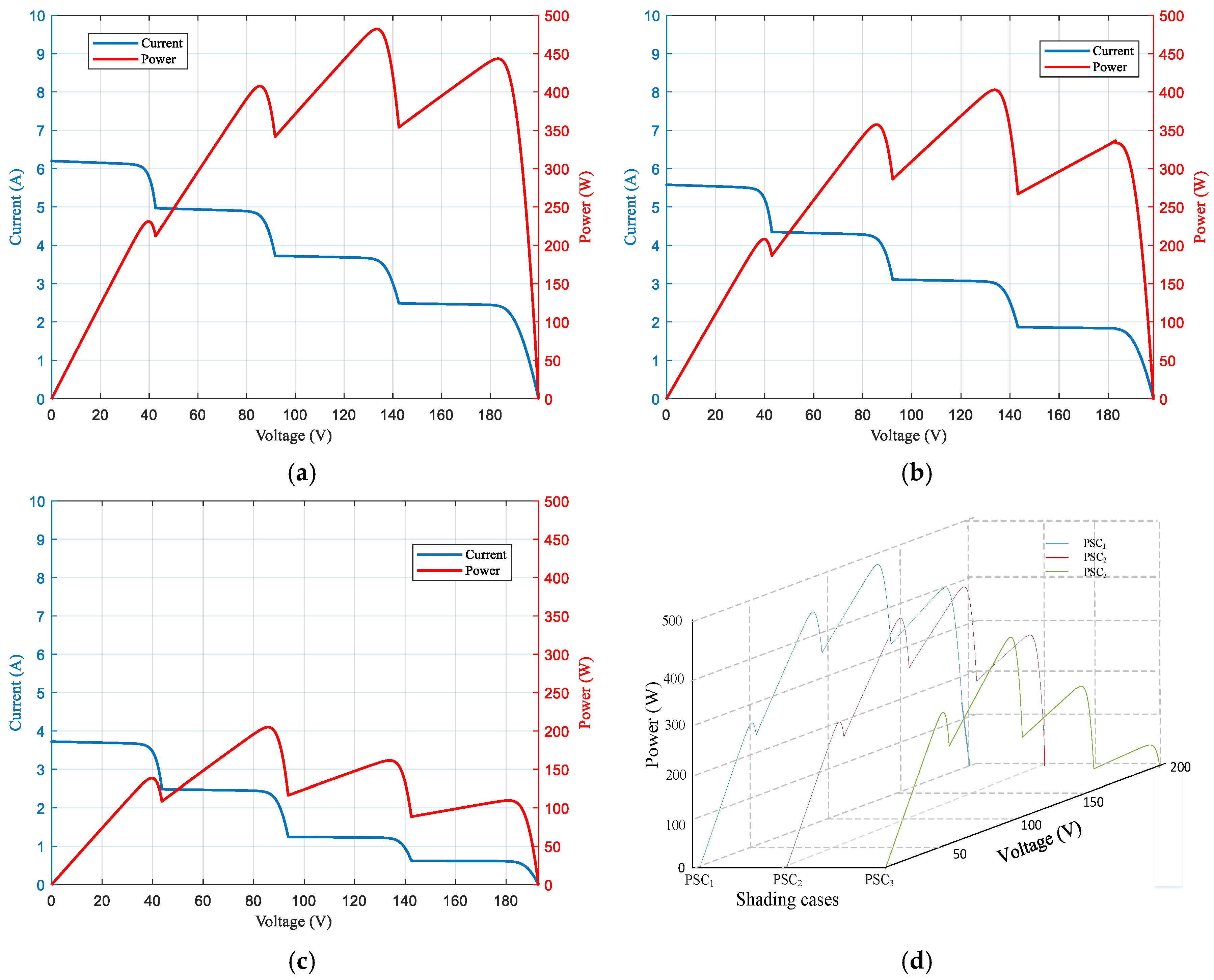
Under PSCs, the solar radiation incident on the PV array is non-uniform, resulting in multiple peaks in the P-V characteristic curve of the PV array as shown in Figure 12. As seen in Figure 12, there are three local MPPs for each of the PSC₁, PSC₂, and PSC₃ scenarios. The GMPP under PSCs occurs at a higher voltage compared to the case of uniform irradiation.

The axis values in Figure 12 are especially maintained constant to allow easy comparison of the power generated in each scenario. As can be seen, as the shading increases and the irradiation decreases, the power produced by the PV array also decreases as expected.

MPP techniques are used to harvest maximum power from the PV array. Most conventional MPPT algorithms are unable to distinguish the GMPP from LMPPs. Hence, intelligent MPPT algorithms are being investigated to more effectively identify the GMPP of a PV array under PSCs. These partially shaded MPPT technologies are designed to ensure maximum power generation from PV arrays under all environmental conditions.

3. Control Principle of PV System

The PV system shown in Figure 13 is constructed with a PV array, a DC–DC boost converter, an MPPT controller, and a PWM signal generator.

The MPPT algorithm works by periodically changing the characteristic variables by slightly increasing or decreasing the parameters until the MPP is reached. To accomplish MPPT, the switching signal with defined duty cycle is obtained by comparing the controller output signal with a high-frequency carrier signal.

Boost Converter

In order to extract maximum power from the PV system, a power conversion circuit must be used. The boost converter is one of the most commonly used converters [26]. The power circuit of a boost converter is shown in Figure 14.

i_pv and v_pv are the current and voltage of the PV system; i_L is the inductor current; i_R and v_R are the load current and voltage, respectively, and u is control signal of the switch S. u = 1, when the switch S is switched on; u = 0, when S is switched off.

According to the switch states, two dynamic mathematical models, one for each state, can be obtained and combined into a state equation as

$${\displaystyle \frac{d{i}_L}{dt}}={\displaystyle \frac{1}{L}}(v_{pv}+\left(u-1\right)v_o$$

(1)

$${\displaystyle \frac{d{v}_o}{dt}}={\displaystyle \frac{1}{C}}(\left(1-u\right)i_L-i_R$$

(2)

in state equation form

$$\left[\begin{array}{c}\dot{i_L}\\ \dot{v_o}\end{array}\right]=\left[\begin{array}{cc}0& -{\displaystyle \frac{1-u}{L}}\\ {\displaystyle \frac{1-u}{C}}& -{\displaystyle \frac{1}{RC}}\end{array}\right]\left[\begin{array}{c}{i}_L\\ v_o\end{array}\right]+\left[\begin{array}{c}{\displaystyle \frac{1}{L}}\\ 0\end{array}\right]v_{pv}$$

(3)

The component values of the PV-fed boost converter were designed based on standard engineering practices to ensure stable operation, high efficiency, and a fast dynamic response under the varying conditions imposed by partial shading.

Specifically, the inductor and capacitor values were determined by the following considerations:

The inductance was selected to maintain continuous conduction mode (CCM) throughout the operating range, thereby reducing current ripple and improving efficiency. The minimum required inductance L_min was calculated using:

$$L_{min}={\displaystyle \frac{v_{pv}\times \left(v_o-v_{pv}\right)}{\Delta I_L\times f_s x v_o}}$$

(4)

where v_pv is the PV array voltage, v_o is the output voltage, ΔI_L is the desired peak-to-peak inductor current ripple (set to approximately 25% of the average input current), and f_s is the switching frequency.

The output capacitor was sized to limit the output voltage ripple to within 1–2% of v_o. The required capacitance was calculated using:

$$C={\displaystyle \frac{i_R\times D}{\Delta v_o\times f_s }}$$

(5)

where i_R is the output current, D is the duty cycle, and Δv_o is the allowable voltage ripple.

Based on these calculations and considering practical component availability and system dynamic requirements, the final component values were determined and used in the simulations in Section 6.

4. PSO Overview

PSO is developed to solve complex optimization problems [27]. It is inspired by the social behavior of birds or fish.

The PSO technique is preferred by researchers, due to its performance, accuracy, and ease of implementation for solving optimization problems in all research fields.

In the PSO technique, the solution of the optimization is defined as particles. The behavior of particles within the swarm is affected by the experiences of the nearby particles.

Each particle is defined by its self-position and velocity and knows the current position and memorizes the self-best solution obtained so far, known as its personal best (p_best). The particles in the entire swarm also know the global best (g_best) solution obtained by the population by using neighborhood topology.

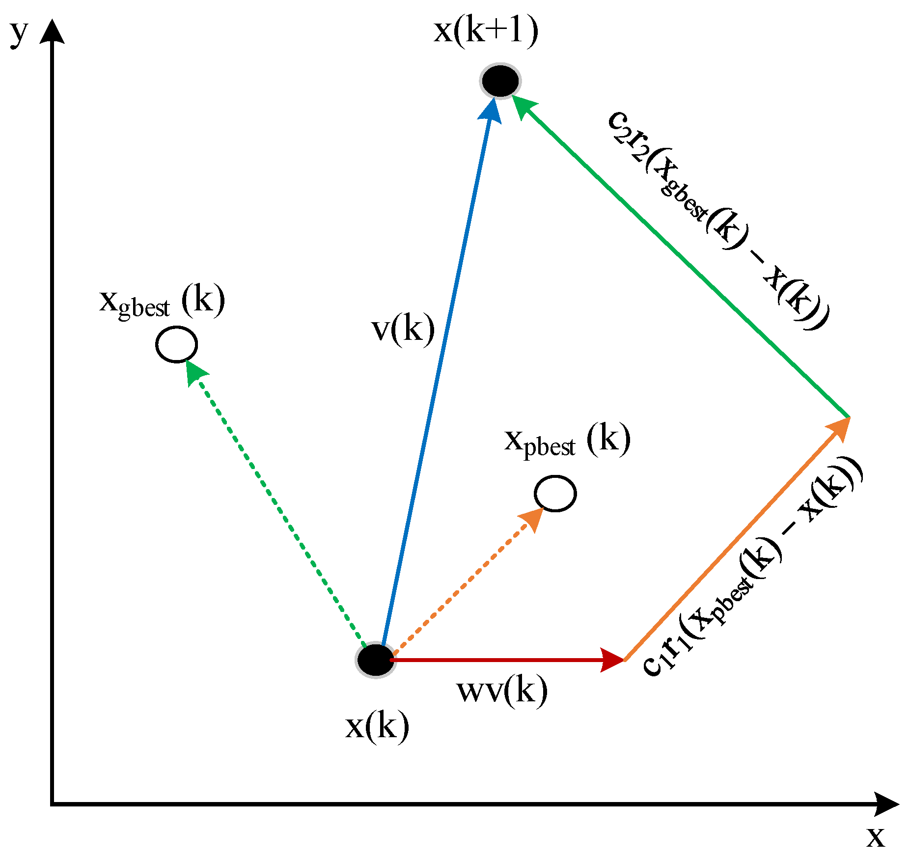
The velocity and position updates for each particle are governed by the following equations, (6) and (7).

$$v_i\left(k+1\right)=w.v_i\left(k\right)+c_1.r_1.\left(pbes{t}_i\left(k\right)-x_i\left(k\right)\right)+c_2.r_2.\left(gbest\left(k\right)-x_i\left(k\right)\right)$$

(6)

$$x_i\left(k+1\right)=x_i\left(k\right)+v_i\left(k+1\right)$$

(7)

where v_i(k) is the velocity of the ith particle at the kth iteration, w is the weight, c₁ and c₂ are acceleration or learning coefficients which are used to direct the search for the local and global optimal solutions, respectively, and r₁ and r₂ are the random values in the range between 0 and 1.

The velocity and position updates are graphically represented in Figure 15.

The velocity update equation balances the particle’s tendency to follow its personal best and the global best positions while considering its previous velocity. This iterative process guides the particles toward the GMPP in the solution space.

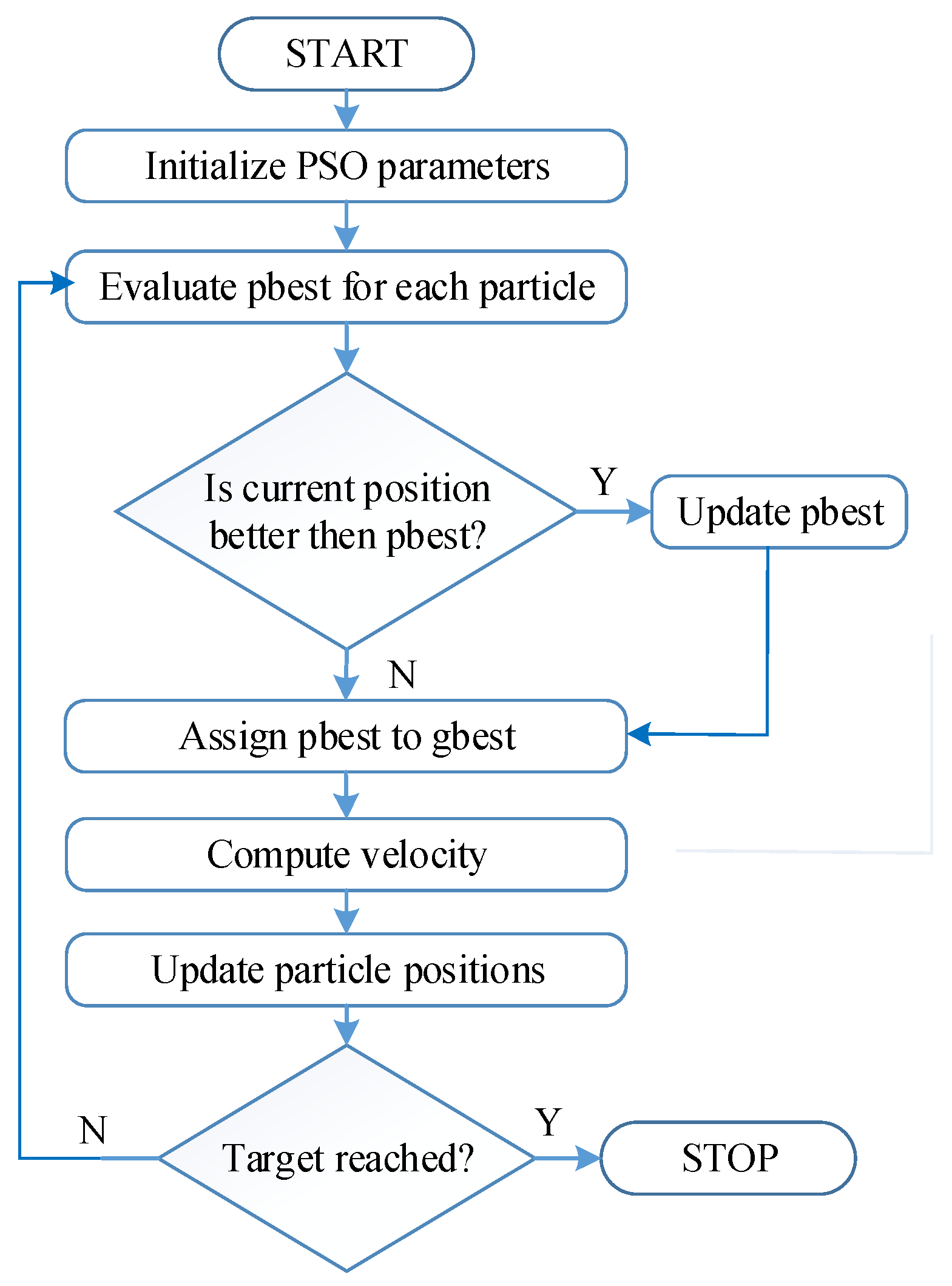
The PSO algorithm is summarized in a flow chart given in Figure 16.

PSO for MPP Tracking

PSO is a popular metaheuristic algorithm used to find the GMPP in PV systems [28]. By applying the PSO algorithm with appropriate parameter settings, the particles in the swarm collectively converge towards the GMPP, optimizing the power output of the PV system.

In this study, the objective function for the PSO algorithm is defined to maximize the output power of the photovoltaic (PV) system under partial shading conditions. The goal is to locate the operating voltage that yields the maximum power output from the PV array. The objective function (OF) is mathematically expressed as:

$$\mathit{max}OF\left(u\right)=P_{pv}\left(u\right)=V_{pv}\times I_{pv}$$

(8)

where u is the control input of the boost converter, P_pv(u) represents the power generated by the PV system, and V_pv(u) and I_pv(u) denote the PV array voltage and current as a function of the control input u.

In the context of MPP tracking, each particle represents a potential operating point of the PV system, typically defined by voltage and current. The PSO algorithm steps for tracking the GMPP can be outlined as follows:

• Initialize a swarm of particles randomly within the specified solution space. Each particle is assigned a random position and velocity.
• Evaluate the fitness (objective function) of each particle. Here the objective is to maximize the power output of the PV system.
• Update the pbest position for each particle based on the evaluation of the fitness function.
• Update the gbest position based on the fitness values obtained by all particles in the swarm.
• Update the velocity and position of each particle using the PSO update equations.
• Repeat steps 3 to 6 until a termination criterion is met.

This balance in the velocity update ensures convergence toward the GMPP by leveraging both local and global knowledge of the solution space. By applying the PSO algorithm with appropriate parameter settings, the particles in the swarm collectively converge towards the GMPP, optimizing the power output of the PV system.

5. Sliding Mode Control Theory

Most control techniques exhibit stability and precision under consistent conditions. However, they tend to struggle with rapidly changing environmental or load conditions. SMC has garnered significant interest in the design of non-linear control systems due to its simplicity, robustness, and favorable dynamic characteristics [29,30]. This method has been applied across various domains, including robotics [31], motor control [32], and inverter control systems [33], to address issues related to parametric variations and both known and unknown disturbances. SMC is grounded in the non-linear control theory established by Utkin in 1977 for variable structure systems [34].

SMC is a robust non-linear control strategy characterized by the formation of a dynamic sliding surface within the state-space domain, representing a specific desired behavior. The system’s trajectory is driven to the sliding surface and constrained to slide along it, enforcing desired performance criteria within this surface. SMC achieves control objectives by imposing a discontinuous control law, typically designed to steer the system towards and maintain it on the sliding surface, thus ensuring a prescribed behavior in the presence of uncertainties, disturbances, and non-linearities.

The key features of SMC include the creation of a well-defined sliding surface, often determined based on system dynamics and desired performance specifications. The control law acts discontinuously, rapidly steering the system towards the sliding surface when outside it, resulting in robust and rapid convergence to the desired behavior. This discontinuity enables resilience against uncertainties and disturbances by ensuring the system behavior is dictated by the sliding surface, thereby improving stability and robustness.

Sliding Mode Control for MPP Tracking

Due to the non-linear behavior of the PV systems, employing a non-linear control strategy is advantageous for tracking the MPP. SMC as applied to MPP tracking in PV systems is a methodological approach aimed at optimizing power extraction from the PV array. The core principle involves the design of a control algorithm to maintain the PV system’s operating point at the MPP of the solar panel’s voltage–current characteristic curve, even in the presence of varying environmental conditions.

In this context, the sliding surface is formulated to represent the difference between the actual operating point of the PV system and the ideal MPP. The control law, designed based on this sliding surface, guides the system dynamics towards the MPP. The discontinuous nature of the control law ensures swift adjustments to bring the system to and maintain it on the sliding surface, which corresponds to the MPP.

By dynamically adjusting the operating point of the PV system based on the sliding surface, SMC minimizes power losses associated with deviations from the MPP caused by changes in solar irradiance, temperature, or partial shading. This precise control mechanism enhances the overall efficiency of the PV system and facilitates the consistent extraction of maximum available power from the solar panels.

Generally, a non-linear time-invariant system is described by the state-space representation as:

$$\dot{x}=f\left(x\right)+g\left(x\right)u$$

(9)

$$y=h\left(x\right)$$

(10)

where x is the state vector, u is the control input vector, y is the output vector, f(x), g(x) and h(x) are the non-linear vector functions representing the dynamics and output equations, respectively.

The goal here is to design a control law such that, given a desired trajectory x_d(t), the tracking error x(t) − x_d(t) tends to zero even in the presence of disturbances. The dynamic behavior of the system can be described by a set of non-linear differential equations derived from the converter and PV module models.

The core idea of the SMC-based MPPT approach is to define a sliding surface that represents the tracking error between the instantaneous PV power and its maximum value. A commonly used sliding surface reaches and remains on a designated sliding surface s, defined by:

$$s\left(t\right)={\displaystyle \frac{d{P}_{pv}\left(t\right)}{dt}}$$

(11)

where P_pv is the output power of the PV array. The system is driven to operate at the point where the derivative of the power with respect to time is zero, which corresponds to the MPP.

The control law is designed to force the sliding variable s(t) to zero in finite time and maintain it there. This is achieved through a discontinuous control input u(t), typically the duty cycle of the boost converter, defined as:

$$u\left(t\right)=u_{eq}\left(t\right)-\lambda sign\left(s\left(t\right)\right)$$

(12)

where u_eq(t) is the equivalent control ensuring sliding mode existence, λ is a positive constant, and sign(s(t)) is the signum function that introduces the switching nature of the control [34].

The sliding mode is characterized by the switching function s(x), which is defined as the distance of the system state from the sliding surface. The procedure followed to define the sliding surface and the control laws for the SMC approach are summarized below:

• Selection of control objective:

The primary control objective is to track the MPP of the PV system by regulating the inductor current of the boost converter. Therefore, the tracking error is defined, based on the difference between the actual inductor current i_L(t) and the reference current I* corresponding to the MPP condition, and this error is used as the switching function.

$$e\left(t\right)=i_L\left(t\right)-I^{*}$$

(13)

2.

Definition of the sliding surface:

The sliding surface is defined to ensure that both the tracking error and its derivative converge to zero. It is defined as:

$$s\left(t\right)={\displaystyle \frac{d}{dt}}e\left(t\right)+\lambda e\left(t\right)=\dot{i_L}+\lambda \left(i_L-I^{*}\right)$$

(14)

where λ is a positive constant that determines the convergence dynamics.

3.

Derivation of system dynamics:

Using the averaged model of the boost converter, the dynamic equation for the inductor current is expressed as:

$${\dot{I}}_L={\displaystyle \frac{1}{L}}\left(v_{pv}-\left(1-u\right)v_o\right)$$

(15)

where v_pv is the PV array voltage, v_o is the output voltage, u is the duty cycle control input, and L is the boost inductor value.

4.

Substitution of the converter dynamics into the sliding surface:

By substituting the converter dynamic model into the sliding surface expression, we obtain:

$$s\left(t\right)={\displaystyle \frac{1}{L}}\left(v_{pv}-\left(1-u\right)v_o\right)+\lambda \left(i_L-I^{*}\right)$$

(16)

5.

Derivation of the equivalent control:

To maintain the system on the sliding surface (i.e., s(t) = 0), the equivalent control u_eq is derived. Using Equation (1) for the converter model and substituting into s(t), and by setting s(t) = 0 and solving for the equivalent control u_eq:

$$u_{eq}=1-{\displaystyle \frac{1}{v_o}}\left(v_{pv}+L\lambda \left(i_L-I^{*}\right)\right)$$

(17)

This control ensures that, once the sliding surface is reached, the system remains on it.

6.

Design of the discontinuous control law:

To enforce finite-time convergence to the sliding surface, a discontinuous switching term is added, resulting in the final control law [35]:

$$u\left(t\right)=u_{eq}\left(t\right)-Ksign\left(s\left(t\right)\right)$$

(18)

where K is a positive design gain that controls the speed of reaching the sliding surface.

7.

Verification of sliding mode existence condition:

The existence condition for the sliding mode, $s\dot{s}<0$, was verified through the reaching law analysis:

$$\mathrm{when} \mathrm{s}\left(\mathrm{t}\right) > 0, \dot{s} \left(t\right) =-\mathrm{Ksign}\left(\mathrm{s}\right(\mathrm{t}\left)\right)-\mathsf{\lambda }\mathrm{s}\left(\mathrm{t}\right) < 0.$$

(19)

$$\mathrm{when} \mathrm{s}\left(\mathrm{t}\right) < 0, \dot{s} \left(t\right)=\mathrm{Ksign}\left(\mathrm{s}\right(\mathrm{t}\left)\right)+\mathsf{\lambda } \left|\mathrm{s}\right(\mathrm{t}\left)\right| > 0.$$

(20)

Thus, the control law guarantees that the system states are driven towards and maintained on the sliding surface.

6. Simulation Results of PSO-Tuned Sliding Mode Based MPPT

PSO can be effectively used to tune the parameters of an SMC strategy for MPP tracking in PV systems [36]. Thus, the advantages of SMC and PSO are combined to achieve efficient MPPT in PV systems. SMC is used to regulate the PV system to its MPP, while PSO is employed to search for the optimal operating point.

By integrating PSO with the SMC-based MPP tracking and tuning its parameters using PSO, the performance and efficiency of the MPP tracking process in a PV system are enhanced.

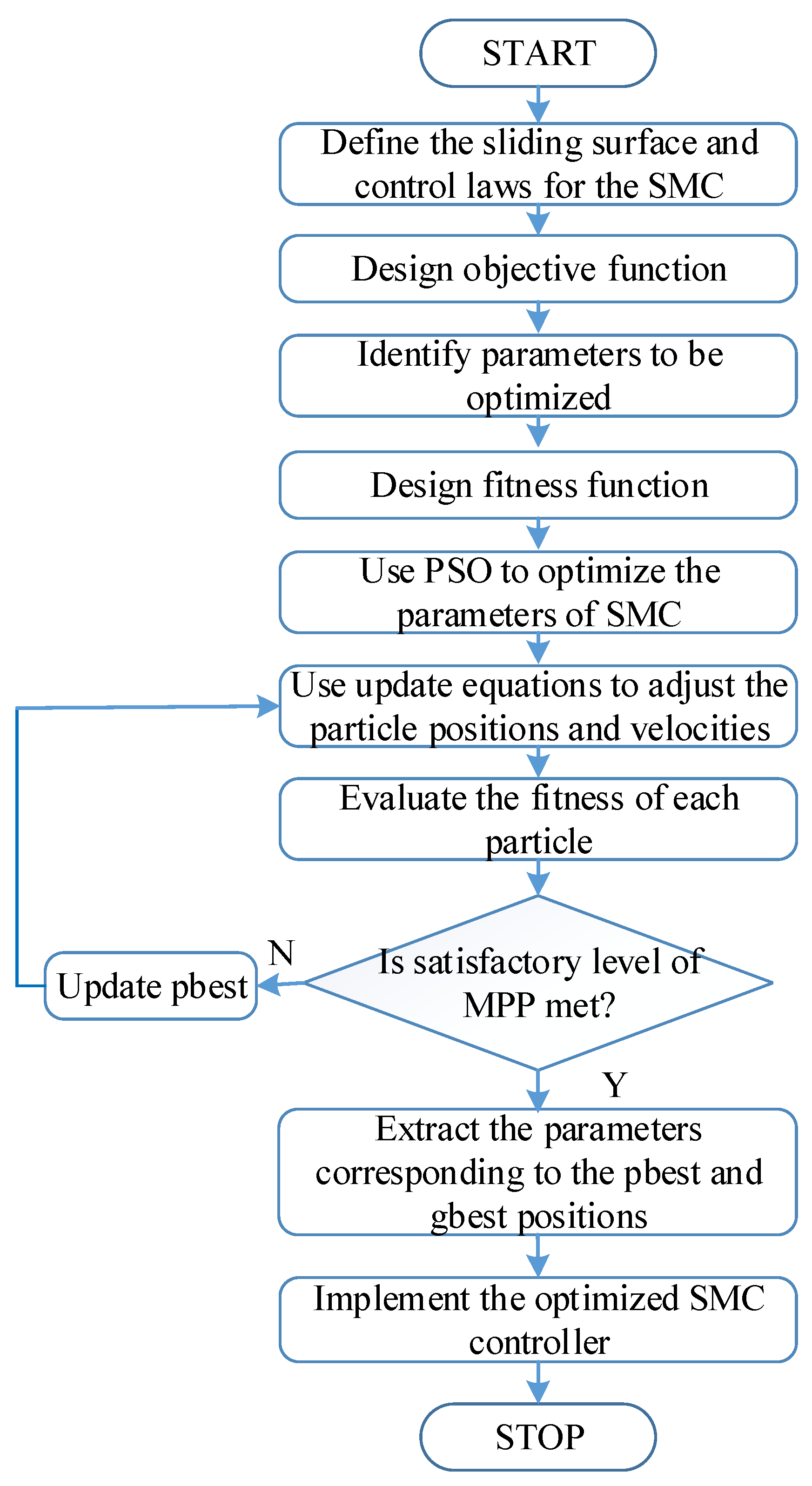
The steps for using PSO to tune the parameters of the SMC-based MPP tracking controller are given in Figure 17.

SMC is advantageous for MPPT in PV systems because it can handle non-linearities and uncertainties in the system, making it robust to variations in solar irradiance, temperature, and other parameters that affect the PV system’s behavior. By adjusting the control signals based on the sliding surface, the system is guided towards the MPP, allowing for efficient power extraction from the PV modules.

The key objective of incorporating PSO into the SMC framework is to automatically and dynamically tune the critical parameters of the SMC controller, specifically the sliding surface slope (λ) and the reaching gain (K). These parameters significantly influence the tracking performance, convergence speed, and robustness. The aim is to regulate the duty cycle such that the output power P_PV is continuously maximized, even under dynamic conditions caused by partial shading, without the need for manual re-adjustment. Thus, the entire control strategy is structured around this optimization objective, ensuring robust and efficient maximum power point tracking under all operating conditions.

The following pseudocode given in Algorithm 1 shows the criterion for tuning SMC. The search objectives are the optimal values of λ and K.

Algorithm 1 Pseudocode for PSO-SMC Tuning

Input: n-particle population Output: Optimal output value       Initialization: position and velocity of each particle for λ and K; LOOP Process 1: for Fitness value calculation to minimize error tracking (OF);       do 2: Update personal and global best (pbest(k) and gbest(k)); 3: end for Meeting stopping criterion; 4: return Optimal output value;

The parameters of the PSO used in the simulations are listed in

Table 3. Parameters of PSO.

Description	Parameter	Value
Number of particles	n	5
Number of iterations	Kmax	10
Cognitive parameter	c1	2
Social parameter	c2	1.8
Weight coefficient	w	0.8

.

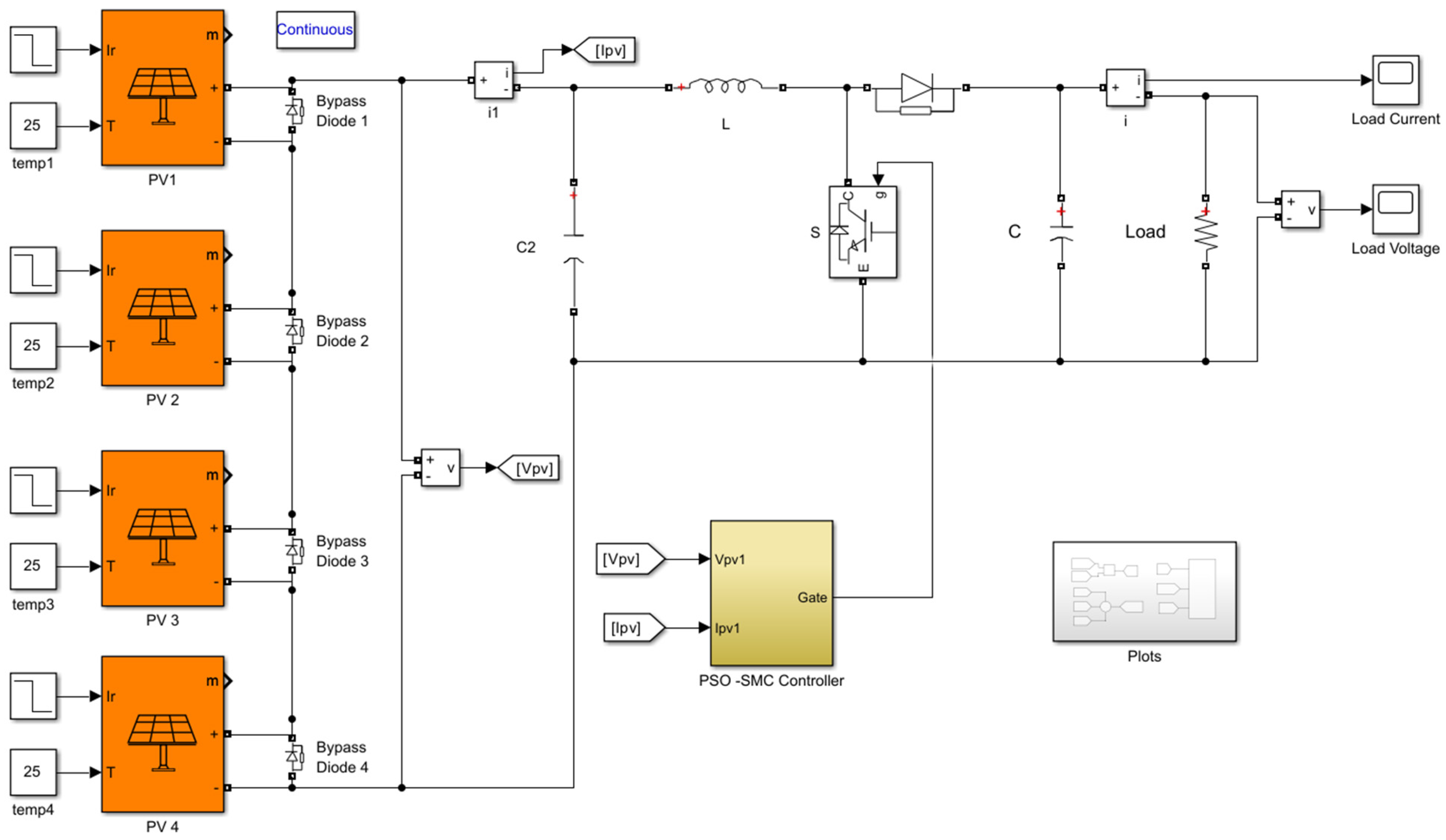
The Simulink model of the developed system is given in Figure 18. The PV module parameters are provided in Table 1, and the boost converter parameters are L = 3 mH, R = 90 Ω, C1 = 100 μF, and C = 200 μF and switching frequency is 5 KHz.

The outcomes of the simulation of the developed Simulink model were analyzed for several PSC scenarios listed in

Table 4. Various PSC scenarios.

		Irradiation (W/m2)
	Time (s)	PV1	PV2	PV3	PV4
PSC1	0–0.2	1000	1000	1000	1000
PSC2	0.2–0.4	800	1000	1000	1000
PSC3	0.4–0.6	800	800	1000	1000
PSC4	0.6–0.8	800	800	700	1000
PSC5	0.8–1.0	800	800	700	500

.

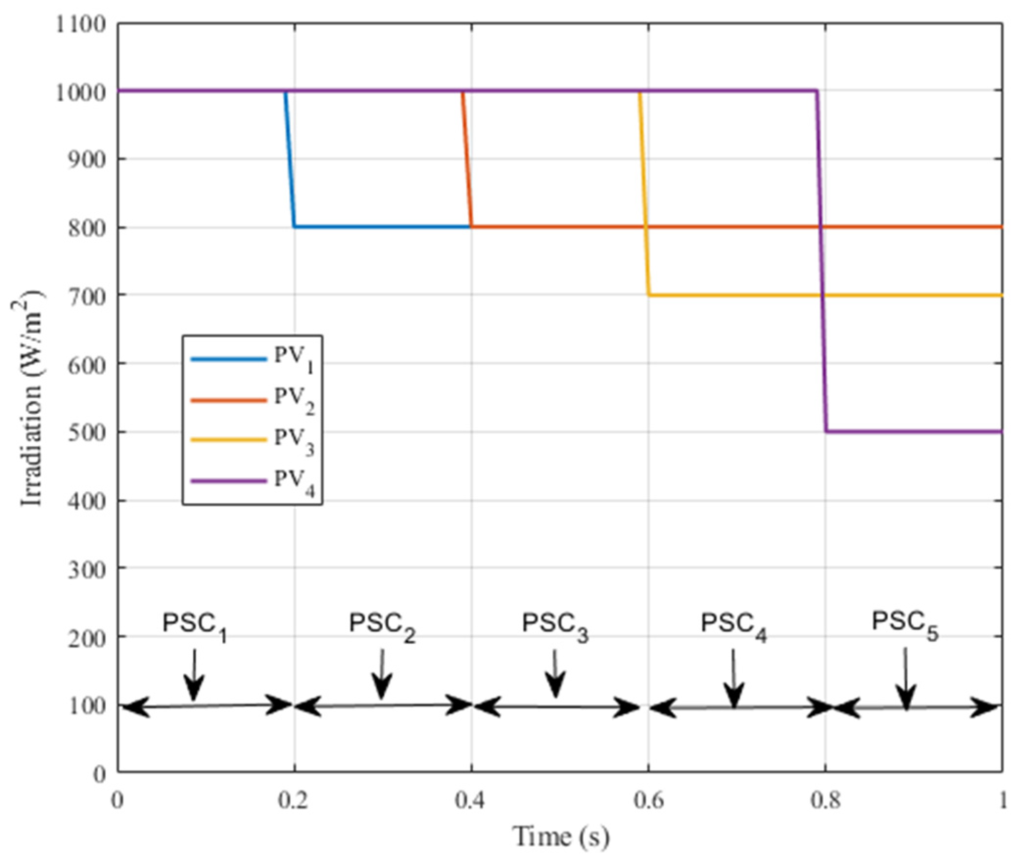
A comparative study, including the proposed PSO-tuned SMC and the standard SMC approach, was conducted under various PS conditions. For that reason, sharp variations in solar irradiation were introduced as shown in Figure 19.

Figure 19 shows the irradiation values for each PV panel during each PSC scenario listed in Table 4. Initially, all four PV panels receive 1000 W/m². At t = 0.2 s, PV₁’s irradiation drops to 800 W/m² while PV₂, PV₃, and PV₄ remain unchanged. At t = 0.4 s, PV₁ remains at 800 W/m², PV₂ falls to 800 W/m², and PV₃ and PV₄ are maintained at 1000 W/m². At t = 0.6, while PV₁ and PV₂ and PV₄ keep the previous irradiation values, PV₃ falls to 700 W/m². At t = 0.8, PV₁, PV₂, and PV₃ remain at the previous values, while PV₄ falls to 500 W/m².

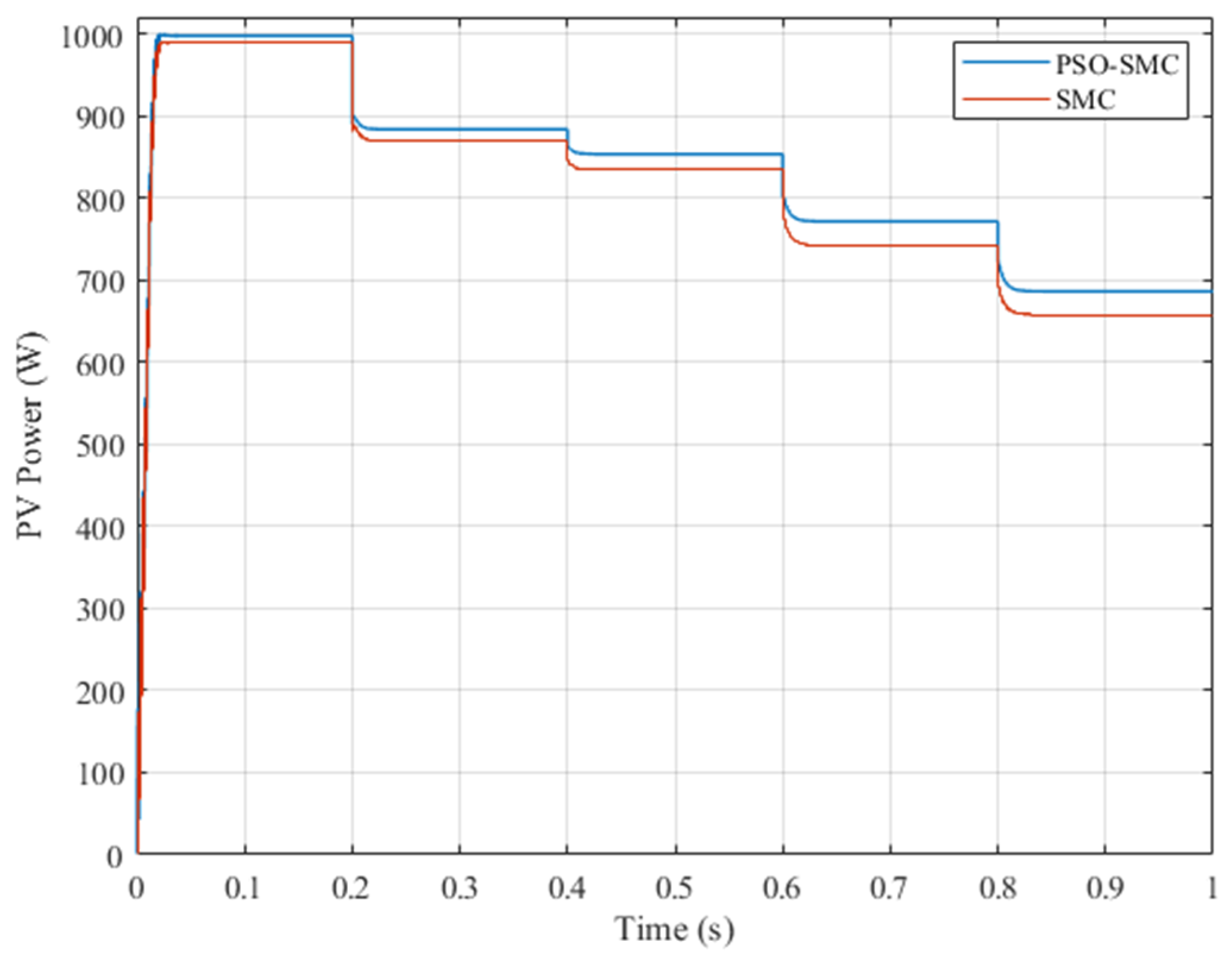
Figure 20 shows PV system power obtained through simulation. The irradiation values representing the PSC scenarios are shown in Figure 19. In this simulation the temperature is kept constant at 25 °C. The produced powers with both SMC and PSO-tuned SMC are represented in this figure. It can be clearly seen that the PV power achieved with the PSO-tuned SMC is higher than that of conventional SMC. It can also be seen that the maximum power is drawn in each PSC scenario.

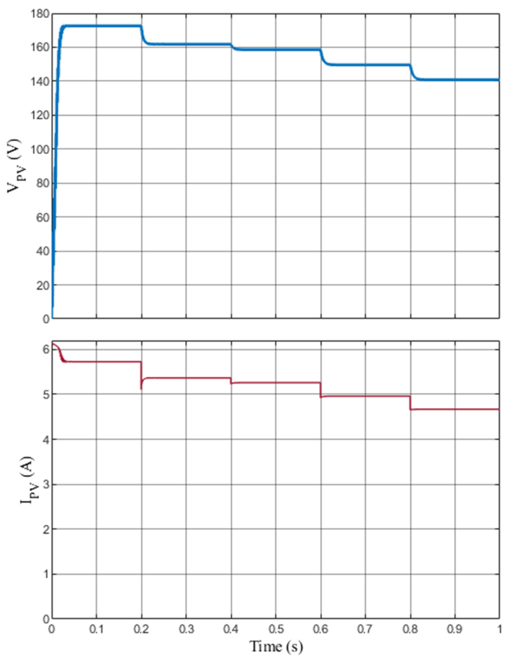
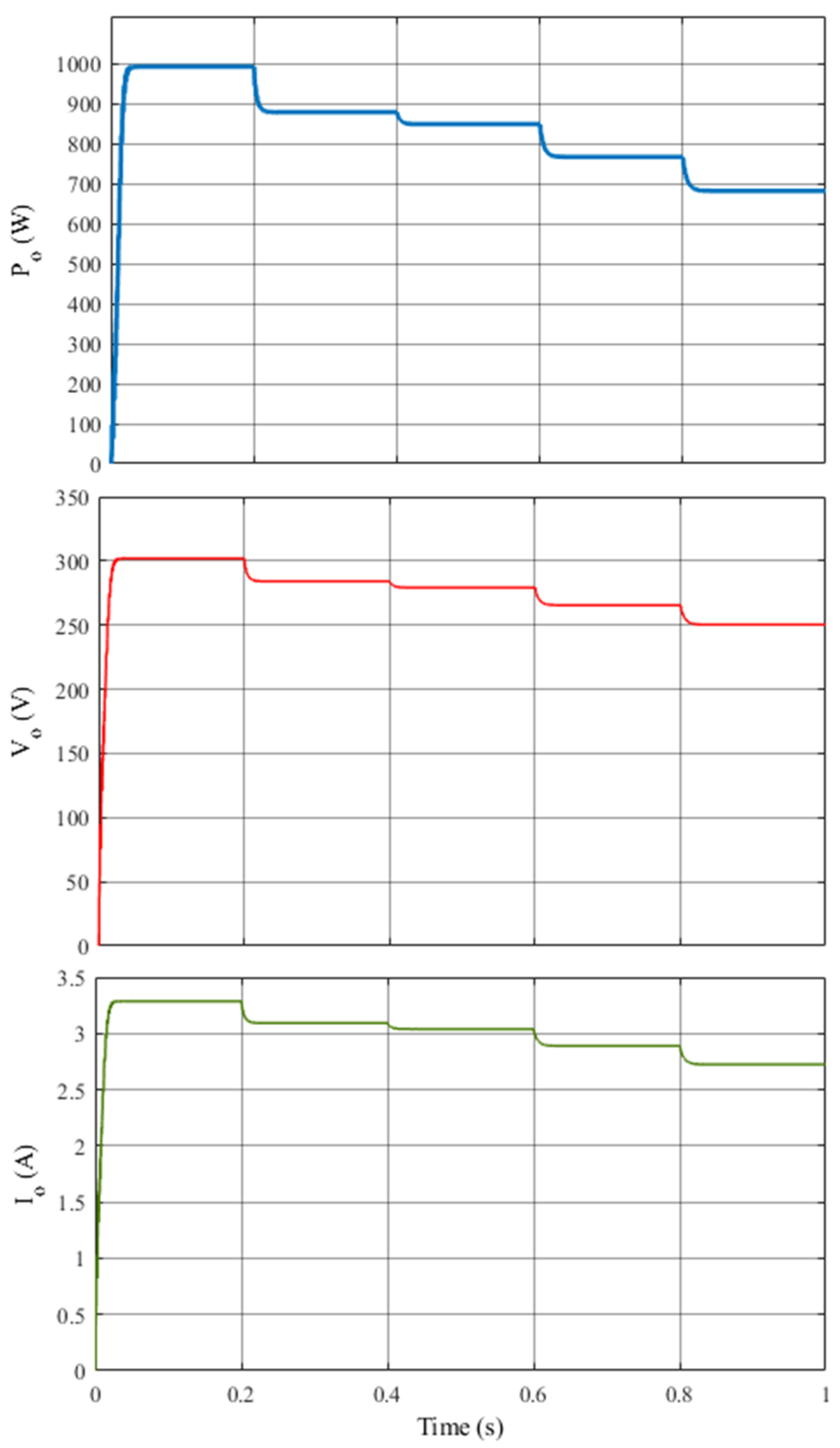
Figure 21 and Figure 22 illustrate the voltage and current generated by the PV system, along with the power, voltage, and current at the load, under the same PSCs presented in Figure 19.

As seen in these figures, maximum power is also transferred to the load, matching the PV system output across all PSC scenarios.

Detailed information regarding the voltage, current, and output power of the PV panel and the associated load under different partial shading scenarios is illustrated in Figure 20, Figure 21 and Figure 22. As is clear, the irradiance, which refers to the amount of solar energy received per unit area on the PV panel surface, plays a crucial role in determining the system’s overall performance.

The voltage, current, and output power provide critical insights into the operational performance and efficiency of the PV system. These parameters serve as essential indicators for assessing the effectiveness of the MPPT algorithm in maximizing energy output and ensuring optimal system behavior. Through detailed analysis, both the control architecture and MPPT strategies can be refined to improve adaptability and performance across a broad range of PSC scenarios. Ultimately, this leads to more efficient energy conversion and better utilization of solar resources.

7. Conclusions

This study presented a hybrid MPPT algorithm for PV systems, which integrates SMC with PSO. The hybrid approach leverages the high-speed convergence and robustness of SMC while addressing its known limitations such as chattering effects and sensitivity to parameter variations through the global search capabilities and adaptive parameter tuning of PSO. This synergy allows for enhanced control precision and improved adaptability under partially shaded or rapidly changing environmental conditions.

Simulation-based performance evaluations demonstrated that the PSO-tuned SMC algorithm exhibits notable superiority over standalone SMC-based controllers. Specifically, the hybrid method achieves improved tracking accuracy, faster transient response, enhanced system stability, and significantly reduced steady-state error. The algorithm continuously optimizes the PV array’s operating point in response to fluctuations in solar irradiance, thereby maximizing power extraction and overall energy conversion efficiency.

Moreover, the PSO-tuned SMC-based MPPT algorithm proved particularly effective under PSCs, where irradiance levels vary rapidly. Simulation results confirm that the method maintains stable performance and high tracking efficiency despite frequent and abrupt irradiance fluctuations. By dynamically adapting control parameters and refining switching behavior, the algorithm ensures smooth convergence to the MPP, minimizing energy loss during transients. As a result, it achieves superior energy harvesting, reduced convergence time, and increased robustness to parameter uncertainties and environmental disturbances.