An Improved Approach for Vehicle Routing Problem with Three-Dimensional Loading Constraints Based on Genetic Algorithm and Residual Space Optimized Strategy

Abstract

To duly and correctly deliver parcels, both the capacity and the delivery route of a delivery vehicle need to be considered. Thus, the delivery process of a delivery vehicle can be characterized as a capacitated vehicle routing problem with three-dimensional loading constraints (3L-CVRP), which is an NP-hard problem. To solve the problem, a mathematical model is established in this paper to minimize the total delivery distance and maximize the loading rate, simultaneously. Additionally, a hybrid algorithm that combines a three-dimensional (3D) packing algorithm based on the residual space optimized (RSO) strategy and an improved genetic algorithm (IGA) is proposed. Initially, the proposed hybrid algorithm employs a modified Clarke–Wright savings algorithm to generate a feasible set of route solutions. Furthermore, building upon the traditional genetic algorithm, an elite retention strategy is introduced, and an enhanced order crossover method is utilized to improve the stability of the hybrid algorithm and its global search capability for optimal solutions. Finally, during each iteration of the algorithm, the RSO algorithm is integrated to verify the feasibility of 3D packing scheme. Two comparative experiments are conducted on 22 modified benchmark instances and actual logistics data of a university against two other algorithms, demonstrating that the proposed RSO-IGA algorithm achieves superior solutions in delivery efficiency.

1. Introduction

Over the past five years, the global logistics industry has undergone a revolutionary digitalization transformation. According to Statista (2024) [1], the global parcel delivery quantity exceeded 150 billion in 2024, with an annual growth rate of 18.7%, and is projected to surge to 350 billion by 2030. In this trend, the optimization goals of logistics systems have shifted from traditional large-scale transportation to high-precision resource coordination [2]. The logistics industry now needs to improve the loading efficiency of individual delivery vehicles while optimizing delivery routes, as the synergy between these two factors directly impacts cost-saving potential.

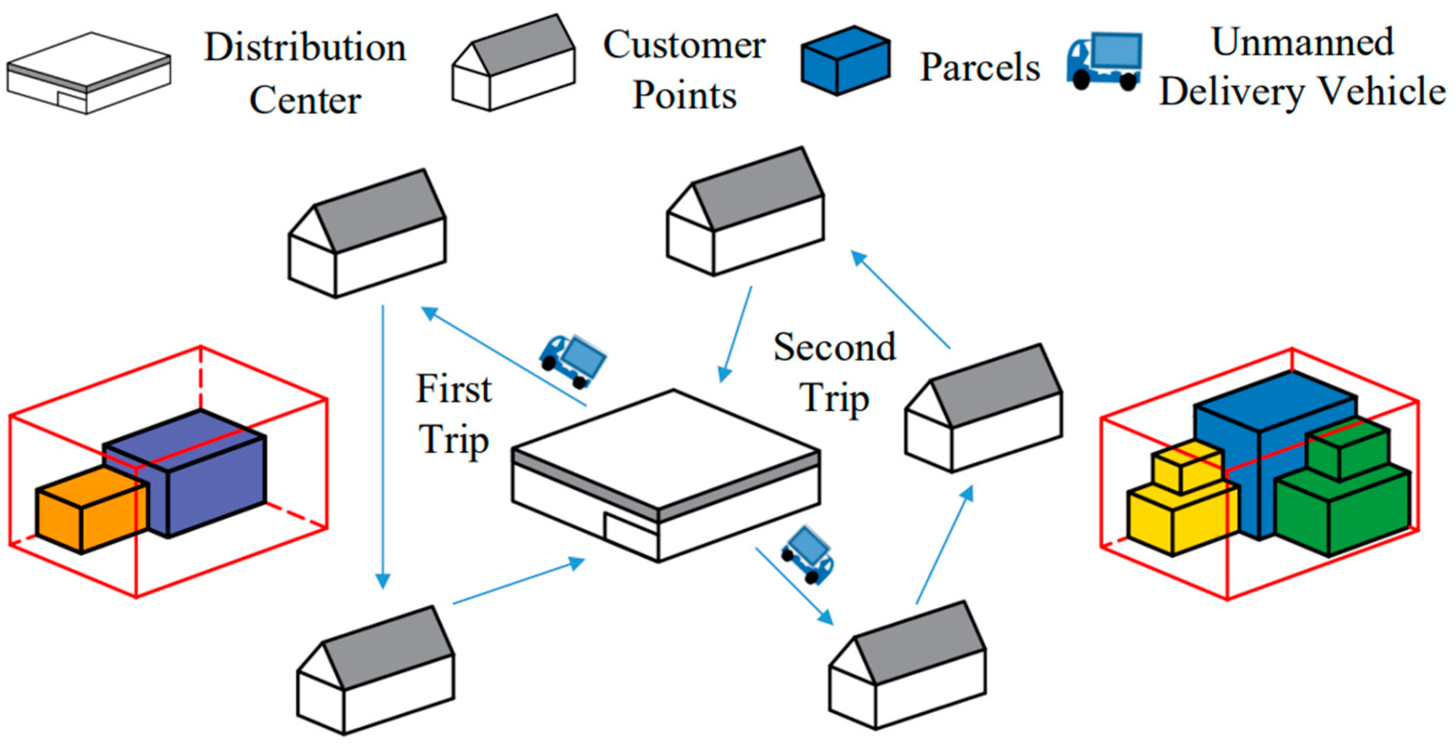
The parcels delivery problem is a common problem of logistics task in factories, hospitals, universities, communities, etc. Raw materials, medicines, and commodities need to be duly and correctly delivered to their destination by a delivery vehicle. Since the capacity and quantity of the delivery vehicles in a delivery center is limited, the delivery scheme should be properly planned to achieve a high delivery efficiency, especially when the parcels are numerous. Generally, as the shape, size, and destination of parcels are different, it is difficult to fully utilize the volume of the delivery vehicle while making sure the vehicle is driving along the shortest delivery route. Therefore, the capacitated vehicle routing problem with three-dimensional loading constraints (3L-CVRP) is an NP-hard problem [3].

The 3L-CVRP research dates back to 2006 when Gendreau et al. [4] proposed a two-stage tabu search algorithm to introduce the rule of last-in-first-out (LIFO) and stability of parcels into route planning. The core value of 3L-CVRP research is achieving Pareto optimality in resource efficiency with limited space and time, and many researchers focused on this point from the aspects of three-dimensional (3D) loading and vehicle route planning. Chi et al. [5] developed two improved relocation constraints to achieve the balance between transportation cost and operational complexity in 3L-CVRP, and the results demonstrate the significance of relocation allowances in reducing overall costs and improving the capacity utilization of the delivery vehicle. Jiang et al. [6] utilized a deep reinforcement learning (DRL) approach to solve the 3D bin packing problem, meaning the parcels loading problem can be solved by sequence, orientation, and position, independently. Similarly, Que et al. [7] proposed a DRL approach to solve the 3D packing problem, and presented a novel state representation of a packing environment. Küçük et al. [8] proposed an approach to program constraints in 3L-CVRP, and improved the results of 36 of 93 benchmark problems. Ribeiro et al. [9] developed a software toolbox to assist in solving the 3D bin packing problem in some specific industries. Li et al. [10,11] deemed that the routing problem is superior to the packing problem, and proposed an adaptive genetic algorithm with elastic strategy to solve the 3L-CVRP for many dynamic demands.

The 3L-CVRP research is significant in the logistics industry, and many constraints can be considered, such as time windows [12,13,14], resource sharing [15], the stability of parcels [16], the heterogeneity of parcels [17], etc. These constraints affect the loading scheme and route planning. Therefore, to simplify the modeling and computing process, many researchers adopt a step-by-step optimization strategy of route planning followed by parcels loading [5] or parcels loading followed by route planning [18]. However, the traditional step-by-step optimization strategy exhibits low efficiency in both steps and low global suboptimality in high-density delivery scenarios (e.g., campus logistics), as the loading sequence and the route topology are nonlinearly correlated [19]. Thus, 3L-CVRP is a multidimensional coupled optimization problem influenced by multiple constraints, and requires a dynamic balance between physical feasibility in 3D space and economic efficiency in the time dimension [20]. Moreover, the complexity of the 3L-CVRP mathematical model grows as O(n³) with the number of customers n. Existing heuristic algorithms face a dilemma: enhancing global search capabilities (e.g., expanding population size) increases the number of 3D packing verifications, while focusing on local search efficiency (e.g., strengthening mutation operators) risks premature convergence. To address 3L-CVRP challenges, existing approaches can be broadly categorized into metaheuristics and hybrid algorithms. The artificial bee colony (ABC) algorithm [21], as a representative swarm intelligence method, has demonstrated promising performance in vehicle routing problems due to its strong global exploration capability. However, its convergence speed tends to degrade when handling multi-layer constraints. Another notable approach is the GA-TS hybrid algorithm, which combines genetic algorithms’ evolutionary mechanisms with tabu search’s local intensification [22]. While this integration improves solution quality, it introduces increased computational complexity that may hinder real-time applications. These inherent limitations in current methodologies motivate our development of the RSO-IGA framework, which aims to synergize the explorative strengths of swarm intelligence with adaptive local search mechanisms while maintaining computational efficiency. Therefore, RSO-IGA is compared with these two algorithms in the following case analysis. The results show that RSO-IGA performs better in express delivery scenarios.

Although the solution set of path length and loading rate can be obtained by using multi-objective optimization, and the internal relationship between path length and loading rate can be clearly seen, the efficiency of this method is low and the calculation time is long. In the actual logistics scenario, we need to obtain a specific optimal delivery scheme (path scheme and packing scheme) in an acceptable calculation time, especially in the circumstances in which the customers have individual requirements. Therefore, this paper adopts the method of multi-objective normalization to solve the problem. This method has a short calculation time and accurate optimal solution, which is suitable for the problem to be solved in this paper. To address these challenges, this study proposes a collaborative optimization framework based on the residual space optimization (RSO) strategy and an improved genetic algorithm (IGA). The innovations of this research are as follows: (1) Introducing a linear weighting method to construct a multi-objective transformation model that integrates packing and route topology features, balancing route economy and loading efficiency. (2) Designing a three-layer encoding system that includes route layer R_chrom, loading layer L_chrom, and orientation layer P_chrom, combining an improved Clarke–Wright algorithm to generate initial solutions and using the Gaode Maps API to obtain real road network distances instead of Manhattan distances. (3) Enhancing the RSO packing scheme through dynamic space partitioning rules and the LIFO constraint reverse verification to ensure the feasibility of 3D loading. Two experiments are conducted based on 22 extended test cases derived from the Cordeau standard dataset and the real logistics data of a Chinese university on a shopping festival. The results show that the proposed approach to 3L-CVRP has practical value in large-scale scenarios.

2. Problem Description and Modeling

2.1. Problem Description

The 3L-CVRP problem can be described as follows: parcels are delivered by delivery vehicles to various customer points (i.e., destinations), all of which constitute a set. Daily orders are fixed and consist of a collection of parcels. The daily delivery plan is determined by the orders and includes multiple delivery routes, each with a unique packing scheme. Each route consists of a group of customer points, and the packing scheme for that route is composed of all the parcels from those customer points. The delivery vehicle departs from the distribution center and executes multiple delivery trips according to the delivery plan. For each trip, the vehicle loads parcels based on the packing scheme and visits the customer points in sequence. After completing a delivery trip (i.e., serving all the customer points assigned to that trip), the vehicle returns to the distribution center and proceeds to the next trip until all the parcels are delivered. Both the parcels and the vehicle compartment are defined as cuboids with three physical dimensions: length, width, and height. As shown in Figure 1, the delivery vehicle performs two delivery trips, serving two and three customer points, respectively. The parcel loading situation is represented by a red rectangle. Parcels of the same color belong to the same customer point, and parcels of different colors belong to different customer points.

Based on this problem, the following assumptions are proposed:

(1)

Single distribution center with multiple trips. There is only one distribution center and one delivery vehicle, and the delivery vehicle can perform multiple delivery trips;

(2)

Static network with fixed daily orders. The vehicle routing network is static, meaning daily order data are fixed and known in advance;

(3)

Regular cuboid shapes for parcels and vehicle compartment. Both the vehicle compartment and parcels are regular cuboids, and the dimensions of any single parcel do not exceed those of the vehicle compartment;

(4)

Orthogonal and non-overlapping packing. Parcels must be placed orthogonally in the compartment without overlapping;

(5)

Vehicle capacity constraint. The total volume of parcels loaded for each trip must not exceed the volume capacity of the vehicle compartment;

(6)

Known distances. The distances between arbitrary two customer points or the distribution center are known;

(7)

No backtracking. To minimize the total travel distance, each customer point is served only once per trip, avoiding “backtracking”;

(8)

Constant speed. Energy consumption and travel costs are not considered, and vehicles travel at a constant speed without traffic delays;

(9)

No time window constraints. Customers can retrieve their parcels from temporary storage areas at customer points, eliminating the need for time window constraints;

(10)

No weight constraints. All the parcels only contain daily necessities, and there are no heavy items, so weight constraints are not considered;

(11)

The shortest path can enable customers to get parcels as soon as possible, which also increases customer satisfaction. The time for customers to take parcels is relatively concentrated, and the traffic situation is smooth during the delivery period, so other soft constraints are not considered.

2.2. Mathematical Model

The goal of this paper is to optimize the delivery distance and vehicle average loading rate simultaneously. Recording a single vehicle loading only increases the algorithm time, so this paper only considers the average loading rate. The symbol definitions are shown in

Table 1. Symbol definitions.

Parameters	Meaning	Parameters	Meaning
i, j, o	Customer ID	b, d	Parcel ID
Bi	Number of parcels required by the i-th customer point	K	Set of vehicle trips
k	Vehicle trip ID	Dij	Distance from customer point i to customer point j
$x_{ij}^k$	Binary variable: equal to 1 if the k-th vehicle trip is from point i to point j; otherwise, 0	$y_{ki}$	Binary variable: equal to 1 if customer point i is served by the k-th vehicle trip; otherwise, 0
f	Total travel distance of the delivery vehicles	M	Node set (including the distribution center and N customer points)
ort	Equal to 1 or 2, representing two placement orientations	N	Customer point set
L, W, H	Length, width, and height of the delivery vehicle compartment	V	Average loading rate of delivery vehicles
lib, lod	Length of the b-th parcel at customer point i and the d-th parcel at customer point o	hib, hod	Height of the b-th parcel at customer point i and the d-th parcel at customer point o
wib, wod	Width of the b-th parcel at customer point i and the d-th parcel at customer point o	$X_{ibk}{,X^{\prime }}_{ibk}{,X}_{odk}{,X^{\prime }}_{odk}$	X-axis coordinates of the bottom-left-rear corner and the opposite corner of the b-th parcel at customer point i and the d-th parcel at customer point o on the k-th trip
$Y_{ibk}{,Y^{\prime }}_{ibk}{,Y}_{odk}{,Y^{\prime }}_{odk}$	Y-axis coordinates of the bottom-left-rear corner and the opposite corner of the b-th parcel at customer point i and the d-th parcel at customer point o on the k-th trip	$Z_{ibk}{,Z^{\prime }}_{ibk}{,Z}_{odk}{,Z^{\prime }}_{odk}$	Z-axis coordinates of the bottom-left-rear corner and the opposite corner of the b-th parcel at customer point i and the d-th parcel at customer point o on the k-th trip

.

The mathematical model is as follows:

(a)

Equation (1) represents the minimization of the total travel distance, as follows:

$$\min \mathrm{f}={\displaystyle {\sum }_{\mathrm{i}\in M}{\displaystyle {\sum }_{j\in M}{\displaystyle {\sum }_{k\in K}\cdot x_{ij}^k}}}\cdot y_{ki}{D}_{ij},i\ne j$$

(1)

(b)

Equation (2) represents the maximization of the average loading rate, as follows:

$$\max V={\displaystyle {\sum }_{k\in K}\frac{{\displaystyle {\sum }_{i\in N}{\displaystyle {\sum }_{b\in B_i}{l}_{ib}{w}_{ib}{h}_{ib}{y}_{ki}}}}{V_k}}$$

(2)

(c)

Equations (3)–(12) are the constraint conditions; Equation (3) ensures that each customer point is served only once per trip, as follows:

$${\displaystyle {\sum }_{i\in N\cup M}{\displaystyle {\sum }_{k\in K}{x}_{ij}^k=1,j\in N}},i\ne j$$

(3)

(d)

Equation (4) specifies that the number of vehicle trips used by the distribution center cannot exceed the total number of elements in set K, as follows:

$${\displaystyle {\sum }_{k\in K}{\displaystyle {\sum }_{i\in N}{x}_{0i}^k}}={\displaystyle {\sum }_{k\in K}{\displaystyle {\sum }_{j\in N}{x}_{j0}^k}}\le \left|K\right|$$

(4)

(e)

Equation (5) represents the flow balance constraint, meaning the inflow and outflow of the same node must be equal, as follows:

$${\displaystyle {\sum }_{i\in M}{x}_{ia}^k}-{\displaystyle {\sum }_{j\in M}{x}_{aj}^k}=0,a\in M,k\in K,i\ne j\ne o$$

(5)

(f)

Equations (6) and (7) represent the uniqueness constraint for flow direction, as follows:

$${\displaystyle {\sum }_{i\in N,i\ne j}{x}_{ij}^k}=y_{kj},j\in N,k\in K$$

(6)

$${\displaystyle {\sum }_{j\in N,j\ne i}{x}_{ij}^k}=y_{ki},i\in N,k\in K$$

(7)

(g)

Equation (8) ensures that the total volume of parcels loaded for each trip does not exceed the volume capacity of the vehicle compartment, as follows:

$${\displaystyle {\sum }_{b\in B_i}{y}_{ki}}\cdot l_{ib}\cdot w_{ib}\cdot h_{ib}\le L\cdot W\cdot H\cdot \alpha ,i\in N,b=\left\{1,2,3,\dots ,B_i\right\},k\in K$$

(8)

(h)

Equation (9) represents the orthogonal placement constraint, where ${\psi x(l}_{ib}{,w}_{ib}{,h}_{ib},ort)$ denotes the length of the edge parallel to the X-axis when the parcel is placed in a specific orientation, as follows:

$${Z^{\prime }}_{ibk}=Z_{ibk}+\psi Z(l_{ib},w_{ib},h_{ib},ort),i\in N,b\in \left\{1,2,3,\dots ,B_i\right\},k\in K$$

(9)

(i)

Equation (10) ensures that parcels are placed inside the compartment and do not exceed its three-dimensional dimensions, as follows:

$${X^{\prime }}_{ibk}<W,{Y^{\prime }}_{ibk}<H,{Z^{\prime }}_{ibk}<L,i\in M,b\in \left\{1,2,3,\dots ,B_i\right\},k\in K$$

(10)

(j)

Equation (11) ensures that no two parcels overlap during loading, as follows:

$$X_{ibk}\ge {X^{\prime }}_{odk}\vee X_{odk}\ge {X^{\prime }}_{ibk}\vee Y_{ibk}\ge {Y^{\prime }}_{odk}\vee Y_{odk}\ge {Y^{\prime }}_{ibk}\vee Z_{ibk}\ge {Z^{\prime }}_{odk}\vee Z_{odk}\ge {Z^{\prime }}_{ibk},k\in K,i,o\in M,b,d\in \left\{1,2,3,\dots ,B_i\right\}$$

(11)

(k)

Equation (12) represents the LIFO principle, meaning parcels are loaded in the reverse order of customer visits, with the assumption that customer point o is served later than customer point i, as follows:

$${X^{\prime }}_{ibk}-{X^{\prime }}_{odk}\ge w_{ib}\vee {Y^{\prime }}_{ibk}-{Y^{\prime }}_{odk}\ge l_{ib}\vee {Z^{\prime }}_{ibk}-{Z^{\prime }}_{odk}\ge h_{ib},k\in K,i,o\in M,b,d\in \left\{1,2,3,\dots ,B_i\right\}$$

(12)

The placement method when ort = 1 is shown by the parcel on the left side of Figure 2, and the placement method when ort = 2 is shown by the parcel on the right side of Figure 2. The bottom-left-back corner point and the diagonal corner point of the parcel within the compartment are illustrated in Figure 2.

In this paper, the two objective functions are transformed into a single objective function. First, Equation (1) is normalized by introducing an initial distance, which is half of the sum of the distances between any two points (including the distribution center and all customer points), denoted as d_total. The total distance saving ratio is then incorporated into the objective function (1). Since the original objective function (1) aims to minimize the total distance, the introduction of the distance saving ratio transforms the objective into maximizing the distance saving ratio. Thus, the objective function is reformulated as follows:

$$\max u={\displaystyle \frac{d_{total}-{\displaystyle {\sum }_{\mathrm{i}\in M}{\displaystyle {\sum }_{j\in M}{\displaystyle {\sum }_{k\in K}\cdot x_{ij}^k}}}\cdot y_{ki}{D}_{ij}}{d_{total}}}$$

(13)

This paper adopts the linear weighting method to simplify the multi-objective optimization problem. By introducing the weighting coefficients ${\lambda }_1$ and ${\lambda }_2$, the transformed single-objective function can be expressed as follows:

$$\max q={\lambda }_{1}u+{\lambda }_{2}V$$

(14)

2.3. AHP-Based Weighting

We structured the weighting process using AHP [23] to formalize the prioritization of objectives, The specific implementation steps are as follows:

Step 1: Expert evaluation and pairwise comparison matrix

We invited a panel of 10 logistics experts from the distribution center of H University to prioritize the objectives, minimizing the total distance and maximizing the average loading rate, and each expert scored independently using Saaty’s 1–9 scale [24]. The details of the specific rating ratio are shown in Appendix A.3. The mean ratings indicate that minimizing examples is considered more critical than maximizing the loading rate, with a consensus ratio of w^agg_A/w^agg_B = 2.33. The resulting pairwise comparison matrix (A) is as follows:

$$A=\left[\begin{array}{cc}1& 2.33\\ 1/2.33& 1\end{array}\right]$$

(15)

Step 2: Weight Calculation and Eigenvalue Validation

The weight vector is derived using the geometric mean method [25], as follows:

1. Compute the geometric mean for each objective, as follows:

$$g_1=\sqrt{1\times 2.33}=1.526,g_2=\sqrt{{\displaystyle \frac{1}{2.33}}\times 1}=0.655$$

(16)

2. Normalize the geometric means to obtain final weights, as follows:

$$\alpha ={\displaystyle \frac{g_1}{g_1+g_2}}={\displaystyle \frac{1.526}{2.181}}\approx 0.699,\beta ={\displaystyle \frac{g_2}{g_1+g_2}}={\displaystyle \frac{0.655}{2.181}}\approx 0.301$$

(17)

To validate the consistency, we calculated the maximum eigenvalue (λ_max), as follows:

1. Compute the weighted sum vector, as follows:

$$Aw=\left[\begin{array}{c}1\times 0.699+2.33\times 0.301\\ {\displaystyle \frac{1}{2.33}}\times 0.699+1\times 0.301\end{array}\right]=\left[\begin{array}{c}1.400\\ 0.601\end{array}\right]$$

(18)

2. Derive λ_max, as follows:

$${\lambda }_{\max }={\displaystyle \frac{1}{2}}({\displaystyle \frac{1.400}{0.699}}+{\displaystyle \frac{0.601}{0.301}})=1.999$$

(19)

3. Verify the consistency, as follows:

$$CI={\displaystyle \frac{{\lambda }_{\max }-n}{n-1}}={\displaystyle \frac{1.999-2}{2-1}}=-0.001$$

(20)

The negative CI value (−0.001) arises from rounding the computed weights (0.699→0.7, 0.301→0.30.) and is mathematically benign for the following reasons:

In AHP, pairwise comparison matrices of size n = 2 are inherently fully consistent if the normalized weights align with the expert-assigned ratio [26]. Here, α/β = 0.7/0.3 ≈ 2.33, directly matching the original pairwise ratio a₁₂ = 2.33. Saaty’s framework does not require a consistency ratio (CR) validation for n = 2, as the random index (RI) is undefined for such cases [27]. In addition, this confirms a perfect consistency. The minor discrepancy (CI = −0.001) solely reflects controlled numerical simplification for practical implementation.

Although the precise AHP calculations yielded weights of α = 0.699 and β = 0.301, these were adjusted to 0.7 and 0.3 to harmonize mathematical rigor with practical feasibility. First, H University’s logistics team advocated for a simplified “70–30” heuristic, reflecting their empirical prioritization of minimizing distance over loading rate. Second, numerical simulations confirmed that rounding introduced negligible deviations (<0.5%) in total distance and loading rate outcomes, ensuring algorithmic robustness. Finally, integer-like coefficients enhance interpretability in industrial settings, avoiding computational complexities associated with fractional weights in real-time routing systems. This adjustment balances precision with usability, maintaining alignment between theoretical methodology and operational realities.

3. Hybrid Algorithm—RSO-IGA

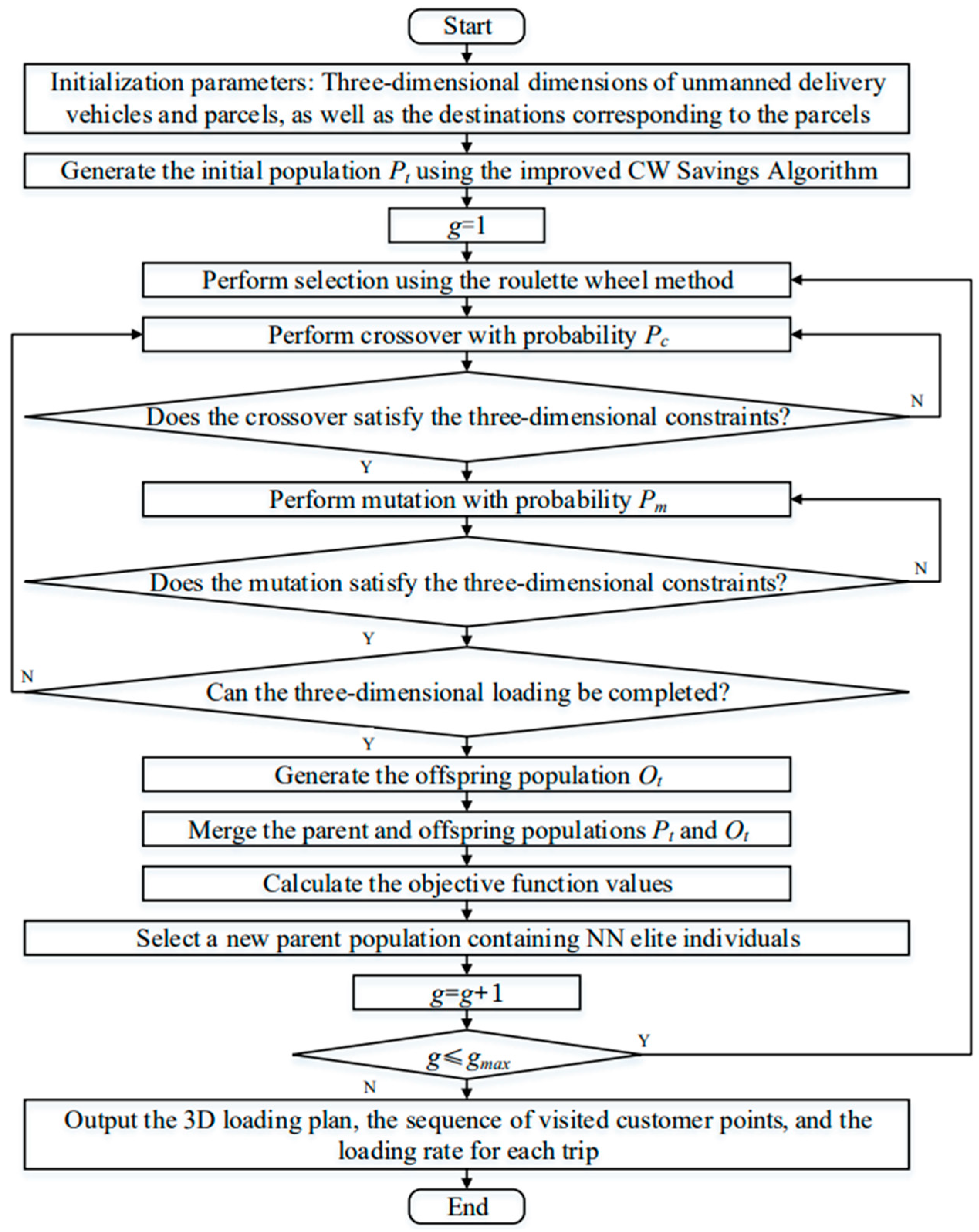
The RSO-IGA algorithm establishes an intrinsic connection between the two subproblems of 3D bin packing and route planning, enabling a more holistic solution for 3L-CVRP. Initially, an improved Clarke–Wright savings algorithm generates route set P_t with 3D constraints as the initial population for the IGA. This enhanced CW algorithm accelerates convergence to optimal solutions, thereby improving computational efficiency.

Set g = 1. Use the roulette wheel selection method in the IGA algorithm to perform selection operations. The selected solutions undergo crossover with probability P_e. The crossed solutions are then subjected to 3D constraint validation. If the constraints are not satisfied, the crossover is repeated; if satisfied, mutation is performed with probability P_m. After mutation, another 3D constraint validation is conducted. Note that the 3D constraints here are distinct from 3D loading constraints. Even if a path plan satisfies Equations (9)–(12), it may not guarantee that all the packages can fit into the delivery vehicle. Therefore, after crossover and mutation in the IGA algorithm, the RSO method is applied to validate 3D loading constraints and eliminate invalid solutions. This step enhances algorithm efficiency by avoiding infeasible solutions that fail loading requirements. The offspring population O_t is merged with parent population P_t, followed by objective function evaluation. An elitism selection mechanism then identifies N elite individuals to form the new parent population. Then, set g = g + 1, and the process iterates until termination criterion g ≤ g_max is met, ultimately outputting the optimized solution. This dual-phase validation mechanism and elite retention strategy effectively balance solution quality and computational efficiency while maintaining 3D feasibility constraints, and the algorithm flow is illustrated in Figure 3.

The specific pseudo-code steps of the hybrid Algorithm 1 are shown below.

Algorithm 1 RSO-IGA Hybrid Algorithm for 3L-CVRP
Input: Customer points D, vehicle dimensions (L, W, H), AHP weights (w1, w2)    Genetic params: pop_size, max_gen, Pc, Pm
Output: Optimized routes R_best with feasible 3D packing schemes
1:	Initialize:
2:	Generate initial population P0 using Improved CW savings algorithm (Algorithm 3)
3:	Decode each individual to routes R_chrom and packing layers (L_chrom, P_chrom)
4:	Validate packing feasibility via RSO Algorithm (Algorithm 2)
5:	for gen = 1 to max_gen do:
6:	# IGA Phase
7:	Elite selection: Preserve top 10% individuals unchanged
8:	Crossover: Improved Order Crossover on P_gen → offspring_Q
9:	Mutation: Swap mutation on offspring_Q → mutated_Q
10:	# RSO Validation Phase
11:	for each individual in mutated_Q:
12:	Decode R_chrom to routes
13:	Apply RSO Algorithm (Algorithm 2) to validate 3D packing feasibility
14:	If infeasible: discard or repair by re-generating L_chrom/P_chrom
15:	# Fitness Evaluation
16:	Calculate fitness via weighted sum:
17:	Fitness = w1 × (normalized_distance) + w2 × (loading_rate)
18:	# Environmental Selection
19:	Combine P_gen + mutated_Q → select next_gen via tournament selection
20:	Return: Best fitness

3.1. Three-Dimensional Bin Packing Algorithm Based on the Residual Space Optimization Strategy

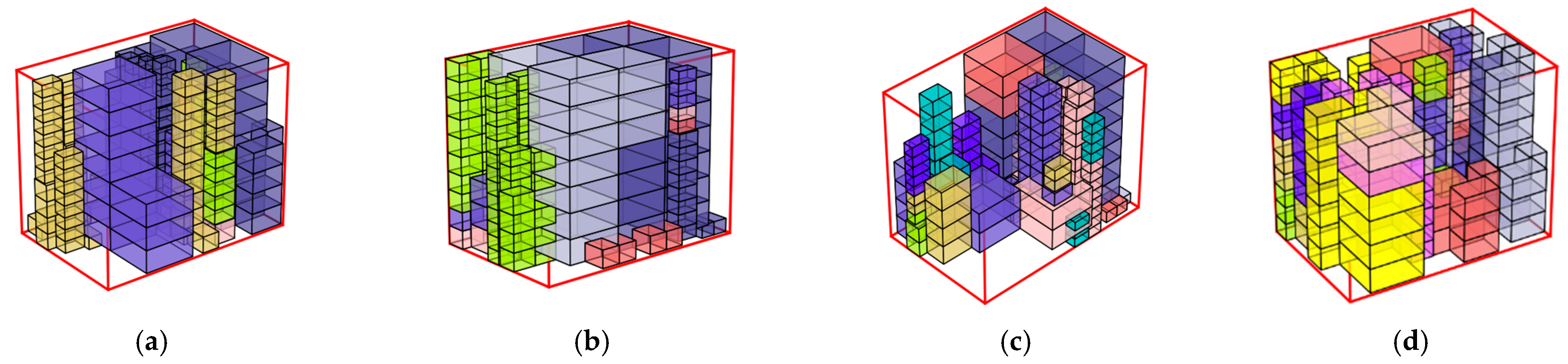
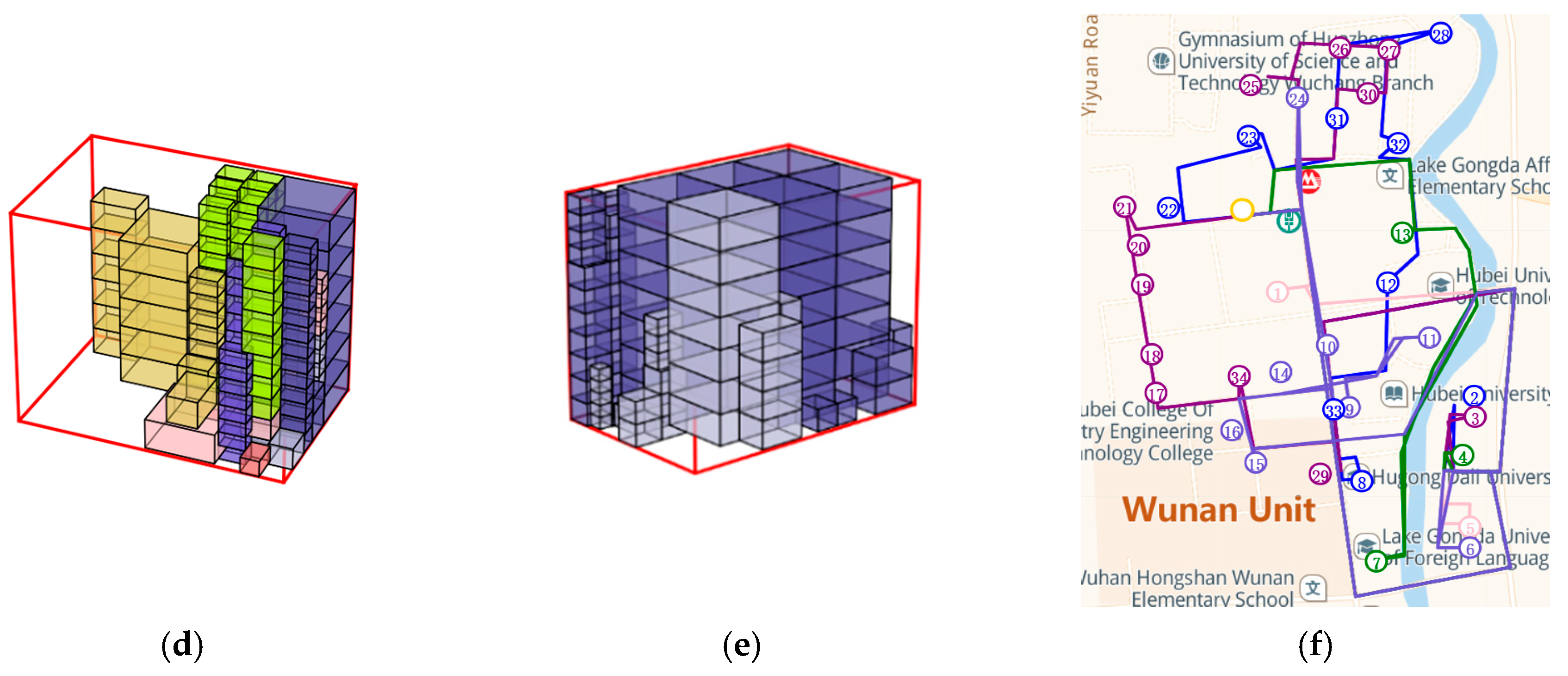
The purpose of three-dimensional bin packing is to verify whether the goods at customer points along the planned route can be loaded into the vehicle under the LIFO constraint. This paper adopts a three-dimensional bin packing algorithm based on the residual space optimization strategy for verification. The packing rules are as follows:

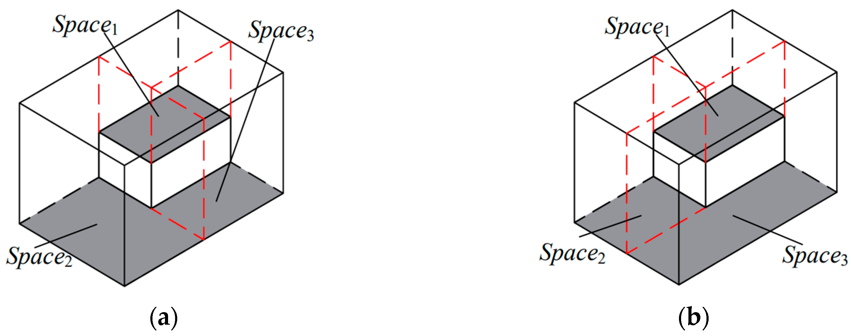
1. Residual space segmentation: As shown in Figure 4, the red dashed lines represent the cutting planes. When horizontal or vertical cutting is applied, the remaining three subspaces are independent of each other. Among them, the subspace Space₁ remains the same under both cutting methods, while Space₂ and Space₃ are subspaces with equal height. The optimization of the residual space segmentation method can be equivalent to the optimization of the residual space in two-dimensional bin packing with height constraints.

2. Parcel placement rules: placing boxes with larger base areas at the bottom ensures better loading capacity for subsequent items. Therefore, under the premise of optimizing residual space, the placement rules are described as follows:

(1)

Sort the parcels based on the size of their base area in descending order, prioritizing the loading of parcels with larger base areas;

(2)

When selecting a placement space, ensure that the space can fully accommodate the parcel, and the difference between the base area of the parcel and the base area of the space should be as small as possible;

(3)

If multiple spaces have base areas similar to that of the current parcel, choose the space that, after accommodating the current parcel, can be divided into the largest possible subspace.

A comprehensive evaluation metric for (2) and (3) is proposed as shown in the following equation:

$$Spac{e}_i\left(l\right)\ge bo{x}_{local}\left(l\right),Spac{e}_i\left(w\right)\ge bo{x}_{local}\left(w\right),Spac{e}_i\left(h\right)\ge bo{x}_{local}\left(h\right)$$

(21)

$$f\left(bo{x}_{local},Spac{e}_i\right)=\left(Spac{e}_i\left(l\right)+bo{x}_{local}\left(l\right)-\gamma \right)\cdot \left(Spac{e}_i\left(w\right)-bo{x}_{local}\left(w\right)+\gamma \right)$$

(22)

Equation (21) indicates that the placement space must be able to accommodate the box. In Equation (22), γ is a correction parameter for the comprehensive evaluation metric, and its value is a positive number significantly smaller than the shortest edge of the smallest parcel. This parameter is introduced to avoid the situation where the comprehensive evaluation metric cannot be optimized when any edge of the placement space equals any edge of the box.

As shown in Figure 5, two identical parcels, b_i and b_j, are loaded into a delivery vehicle. Without the correction parameter, the comprehensive evaluation metrics f(b_j,Space₁) and f(b_j,Space₃) would both be 0. According to placement rule (3), the spatial configuration shown in Figure 5a is obtained.

When the correction parameter is included, the comprehensive evaluation metrics are calculated as f(b_j,Space₁) = −γ² and f(b_j,Space₃) = −γ∙(Space₃ (l) − b_j(l)). Clearly, the former is larger, resulting in the spatial configuration shown in Figure 5b. From Figure 5, it is evident that the corrected residual space set provides more valuable reference for subsequent packing.

The specific pseudocode steps of the remaining space optimization Algorithm 2 are as follows:

Algorithm 2 RSO 3D Packing Validation
Input: Route R, parcels list with dimensions, LIFO stack order
Output: Packing feasibility (True/False), loading rate V
1:	Initialize:
2:	Residual spaces: [Space0 = (L, W, H, corner = (0,0,0))]
3:	Space_avi = True # Space availability flag, initially True
4:	Plan_list = [] # List to store packing plans, initially empty
5:	Sort parcels by base area (largest-first) and push to LIFO stack
6:	Sort parcels: Sort by base area descending order, then push to LIFO stack
7:	Update residual spaces and total space count:
8:	Update Space_list (list of available spaces)
9:	Total number of available spaces: num_S
10:	Main Packing Loop:
11:	while parcels exist in LIFO stack:
12:	a. Pop the next parcel p from stack
14:	b. For each Space in residual_spaces:
15:	Calculate placement score f(p, Space) based on Equations (15) and (16)
16:	f(p, Space) represents the placement score, a measure of how well parcel p fits in the given space
17:	c. If f > 0: # Placement is feasible
18:	Place parcel p in the space with the highest f value
19:	Split residual space into 3 subspaces (based on current parcel placement)
20:	Update residual_spaces with new subspaces (Figure 4)
21:	Increment placement counter (s = s + 1)
22:	d. If no further feasible placements are found for parcel p in the current residual spaces:
23:	Break out of the loop (to check the next parcel)
24:	If no feasible placement (space) is found for a parcel:
25:	Return False (packing not possible)
26:	If all parcels are successfully placed:
27:	Calculate the loading rate V = total_parcel_volume/(L × W × H)
28:	Return True (packing is successful), V (loading rate)
29:	End Algorithm

3. LIFO constraint: campus parcel delivery must consider the order of customer logistics distribution, so it is not possible to sort all goods uniformly. The path plan is reversed and then sequentially pushed onto a stack. When popping elements from the stack, they are removed starting from the top element, ensuring that the order of elements popped matches the sequence of customer points in the path plan.

3.2. IGA Algorithm

3.2.1. Encoding and Decoding

(1)

Encoding

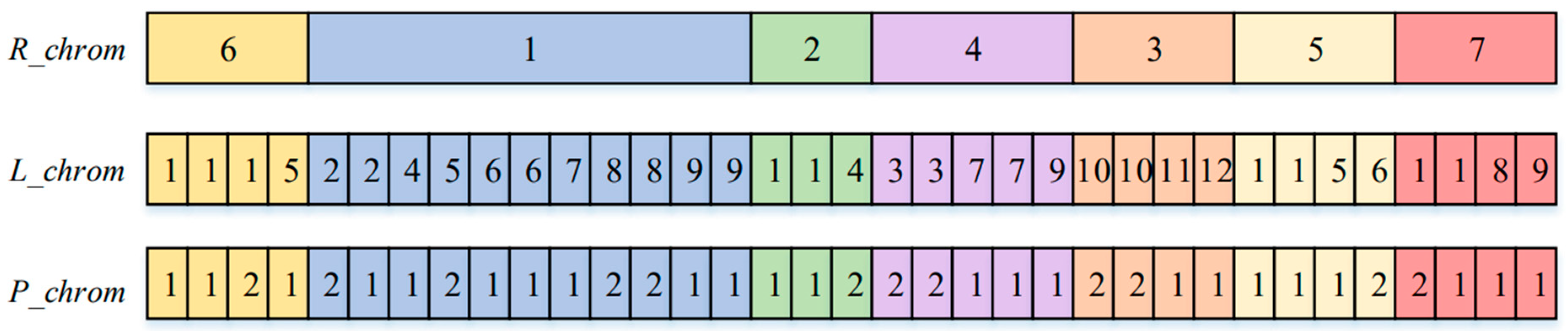
The encoding part requires that the chromosome contains all the basic information of an individual. Currently, the most common encoding method for solving vehicle routing problems is real-number encoding, which encodes the visiting sequence of customer points. The solution space is the full permutation of the visiting sequence, and the corresponding space complexity is related to the number of customer points. However, this paper also needs to consider three-dimensional loading constraints and the practical conditions of campus delivery. Therefore, while considering the route as the visiting sequence, a three-layer real-number encoding method is adopted. As shown in Figure 6, a simple schematic diagram of the three-layer encoding method is provided.

The first layer, R_chrom, represents the route encoding. The sequence reflects the order in which the delivery vehicle visits the customer points, and the numbers correspond to the sequential indices of the customer points.

The second layer, L-chrom, represents the loading sequence. The sequence indicates the order in which parcels are loaded, and the numbers correspond to the parcel demand indices associated with R_chrom.

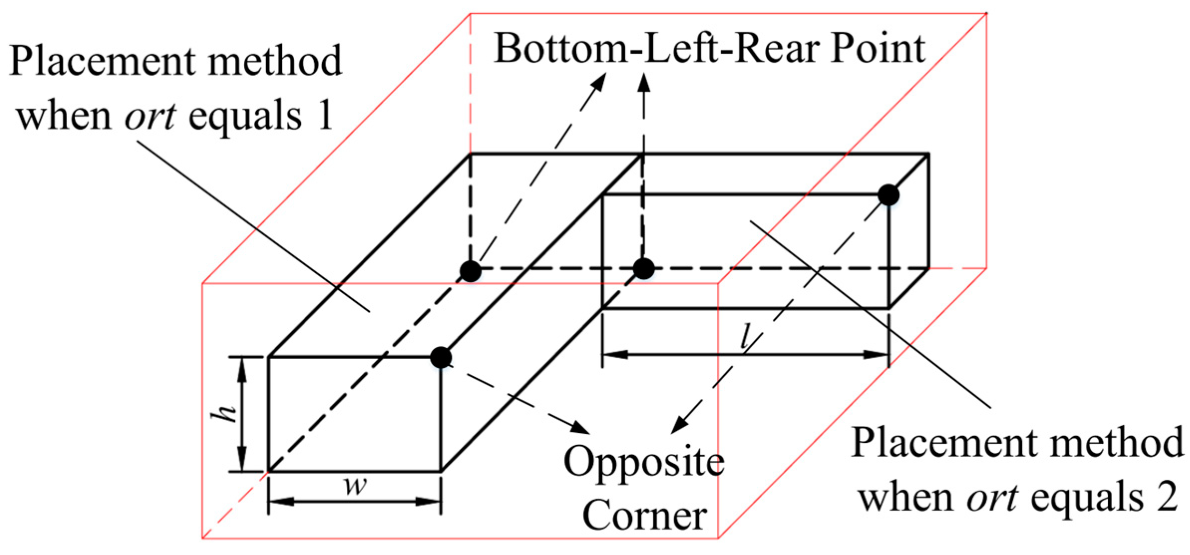
The third layer, P_chrom, represents the parcel placement encoding. The numbers correspond to the placement methods of the parcels in the vehicle, where only two placement methods are considered for the parcels in the vehicle.

(2)

Decoding

The decoding process involves transforming the solution represented by the encoding into specific executable operational steps. For the three-layer encoding method proposed in this paper, since the R_chrom layer represents the vehicle’s visiting sequence, the legality of the route must be ensured during the decoding of the R_chrom layer. This requires considering the impact of three-dimensional constraints on the route. Therefore, under loading constraints, the route needs to be divided into multiple sub-routes, and a “0 gene” is added at the beginning and end of each sub-route to represent a complete delivery route for the delivery vehicle. Additionally, to obtain valid solutions, the L_chrom and P_chrom layers must undergo three-dimensional constraint verification during each decoding step.

As shown in Figure 7, the red dashed line represents the pass segmentation. The first route is “0→6→1→2→4→0,” and the second route is “0→3→5→7→0.” By repeating the above decoding process, the route plan for each trip of the delivery vehicle under this individual can be restored.

3.2.2. Introduction of the Improved CW Savings Algorithm

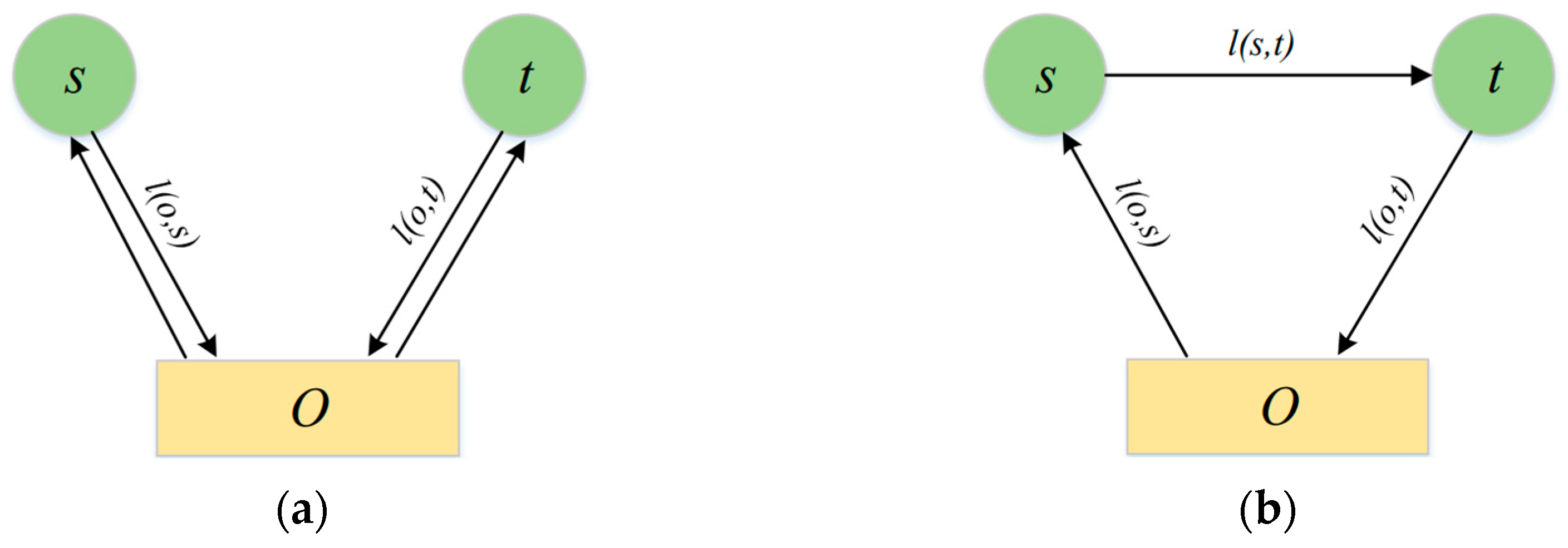
To more effectively converge to the optimal solution, the CW savings algorithm is introduced, and the solution generated by the CW savings algorithm is used as the initial solution. The core idea of the CW algorithm is to calculate and compare the “savings” between different customer points, which refers to the distance saved by merging two customer points into the same route, thereby gradually constructing the optimal route. The initial solution is direct delivery, where a single vehicle serves each customer point separately. Although the initial solution can meet the required cargo demands, it results in excessive vehicle trips, long delivery routes, and low loading rates.

In the CW Algorithm, the “savings” are illustrated in Figure 8. Customer points s and t are served by the distribution center o. Here, l(o, s) and l(o, t) represent the shortest feasible distances from the distribution center to customer points s and t, respectively, and l(s, t) represents the shortest feasible distance between customer points s and t. The savings from merging customer points s and t is calculated as |l(s, t) + l(o, s) + l(o, t) − 2(l(o, s) + l(o, t))|.

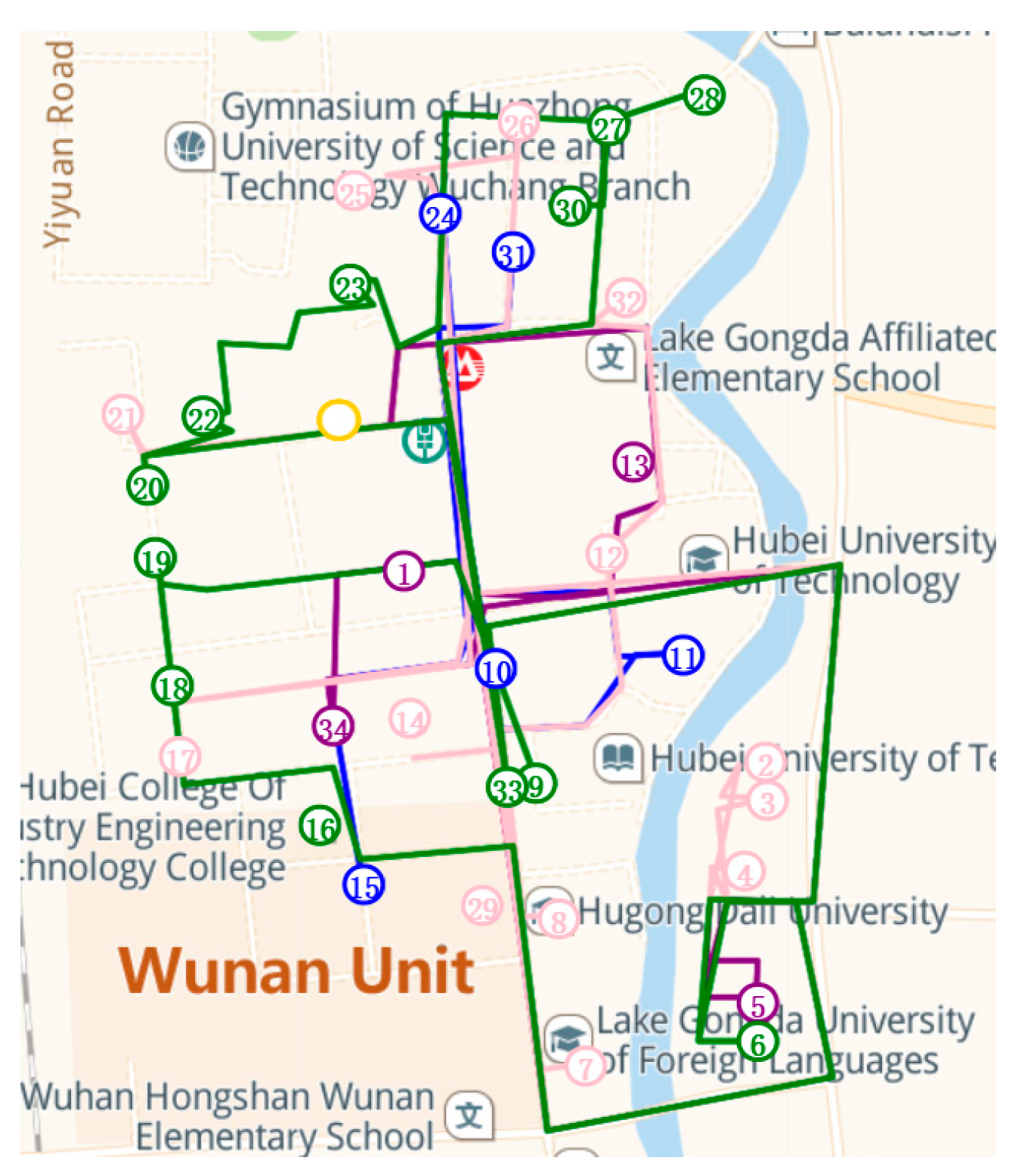
In the traditional CW savings algorithm, l(o, s), l(o, t), and l(s, t) are calculated using the Manhattan distance equation. However, in the context of a campus environment, the routes are more complex. Therefore, this paper utilizes the Gaode Maps API to calculate the actual road distances based on latitude and longitude rather than simple straight-line distances. The improved CW savings algorithm is implemented as follows:

(1)

Initialization: calculate the distance matrix D for all customer points and set the initial solution as individual routes containing the distribution center and each customer point;

(2)

Calculate savings: based on the distance matrix D, compute the savings between all customer points and construct the savings matrix S;

(3)

Sort savings: sort the savings matrix S in descending order to obtain the savings list L;

(4)

Merge savings: randomly select a customer point and, following the order of the savings list L, sequentially check whether merging the next customer point satisfies the three-dimensional constraints. If not, skip that customer point and proceed to the next;

(5)

Update routes: after each successful merge, update the current route and the set of unvisited customer points;

(6)

Termination: the algorithm terminates when all customer points have been visited.

The improved CW savings algorithm generates feasible solutions during the route merging process and evaluates the distance savings. Simultaneously, it assesses the feasibility of merging routes based on three-dimensional constraints. As a result, the initial solutions generated by the improved CW savings algorithm are feasible and stable, facilitating the optimization of feasible solutions in the second stage using the improved GA.

Unlike the traditional GA, which employs a random strategy to generate the initial population, the introduction of the CW savings algorithm provides better initial solutions, aiding convergence to the optimal solution. Additionally, the elite retention strategy is incorporated to ensure that a certain number of elite individuals are preserved during the iteration process, thereby improving the accuracy of the optimization results. Therefore, compared to the traditional GA, the proposed IGA combines the improved CW savings algorithm and the elite retention strategy, enhancing the stability of the hybrid algorithm and its global search capability for finding optimal solutions.

The specific pseudocode of the improved CW savings Algorithm 3 is as follows:

Algorithm 3 Improved CW-Savings Algorithm
1:	Calculate real-road distances using Gaode Maps API
2:	Initialize: Each customer as separate route [0, i, 0]
3:	Compute savings S_ij = distance(0,i) + distance(0,j) − distance(i,j)
4:	Sort S_ij in descending order
5:	For each S_ij in sorted list:
6:	Merge routes containing i and j if:
7:	Capacity constraint satisfied (Equation (8))
8:	3D packing validated by RSO (Algorithm 2)
9:	Return: Feasible initial routes

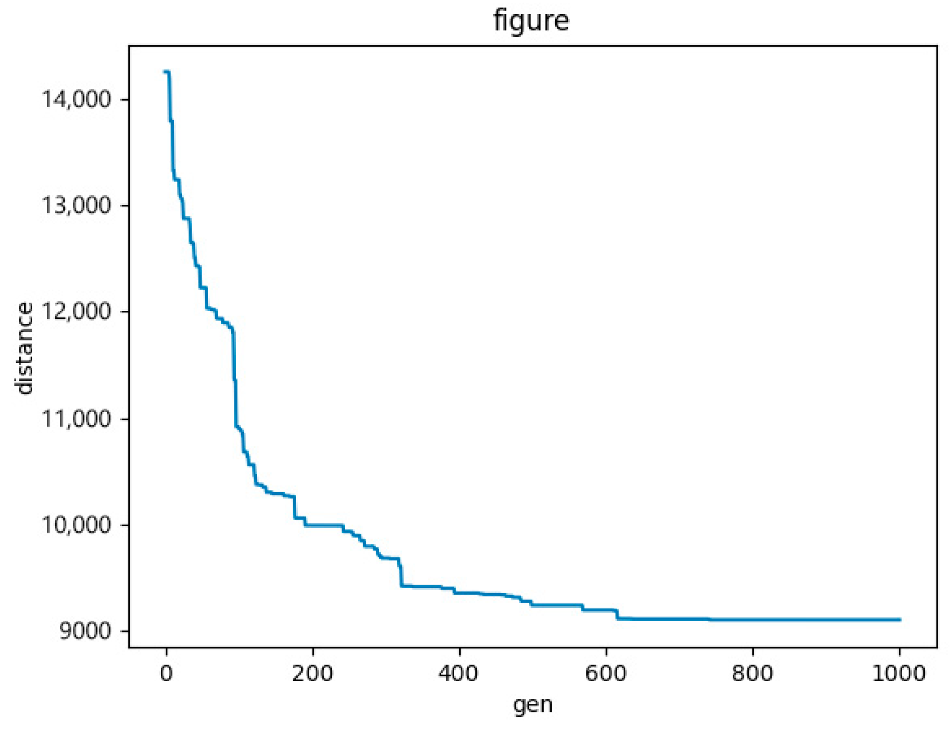
Fitness Function Construction: The optimization objectives in this study are to minimize the route length and maximize the average loading rate. During the population iteration process, the route length is expected to decrease gradually until the optimal solution is reached. In the population evolution process, individuals with higher fitness values are more likely to be retained. The fitness function is defined as in Equation (23):

$$F=-{\lambda }_{1}u+{\lambda }_{2}V$$

(23)

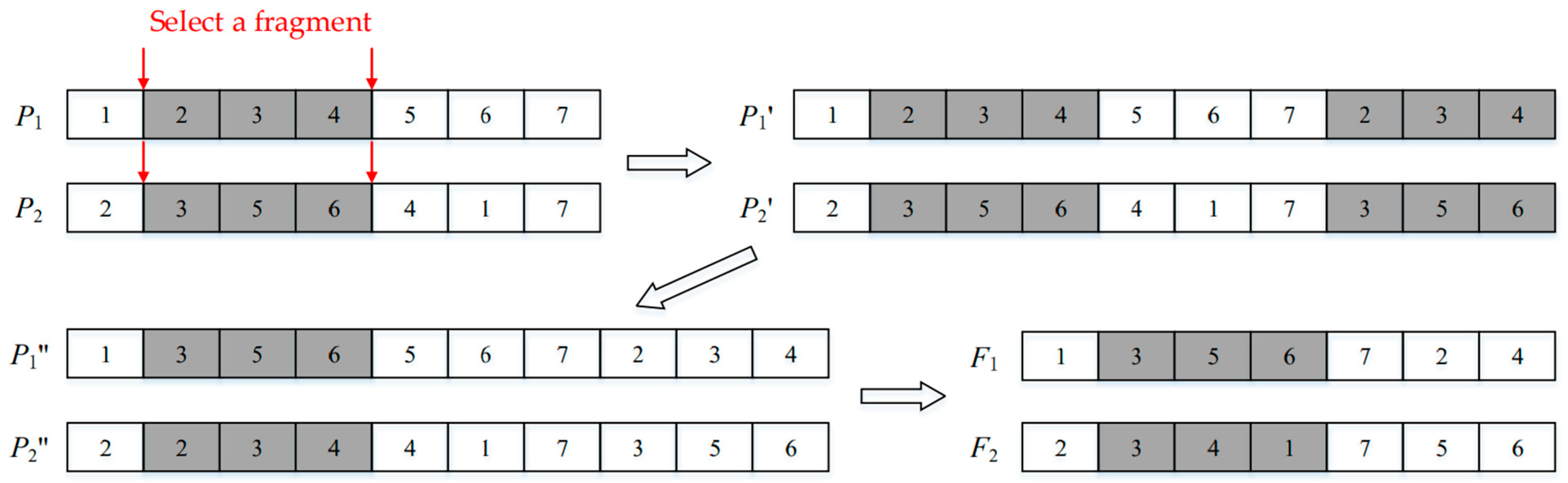
3.2.3. Crossover

This paper employs an improved order crossover method. The specific steps are as follows:

(1)

Select the same region on two parent chromosomes, P₁ and P₂;

(2)

Copy the genes from the selected region of P₁ and P₂ to the end of P₁ and P₂, respectively, resulting in P_1′ and P_2′;

(3)

Exchange the genes in the selected regions of P_1′ and P_2′, resulting in P_1″ and P_2″;

(4)

Remove the duplicate genes outside the selected regions in P_1″ and P_2″, yielding two offspring chromosomes, F₁ and F₂. The specific operation is illustrated in Figure 9.

In Figure 9, the red arrow represents the segmentation of chromosome fragments, and the white arrow represents the change process of chromosome. After completing the crossover operation, it is necessary to verify whether the loading plan of the delivery vehicle satisfies the three-dimensional constraints. If not, the crossover operation is repeated.

3.2.4. Mutation

A chromosome is randomly selected from the population generated after the crossover operation for mutation. The mutation process is illustrated in Figure 10, the red arrow indicates the exchange of fragments of two chromosomes, and the white arrow indicates the change process of the whole chromosome. The steps are as follows:

(1)

Select some chromosomes from the parent generation based on the mutation probability;

(2)

Randomly select two genes from the parent chromosome and exchange them to produce a new offspring chromosome;

(3)

Verify whether the loading plan of the delivery vehicle after the mutation operation satisfies the three-dimensional constraints. If not, the mutation operation is repeated.

The offspring generated after crossover and mutation are validated using the residual space-optimized three-dimensional bin packing algorithm to determine whether the plan can accommodate all parcels along the route. If successful, subsequent operations are performed; otherwise, the crossover and mutation operations are repeated.

3.3. Algorithm Comparison

This paper further modifies the experimental data based on the following instances designed by Cordeau:

(1)

The number of customer points is increased;

(2)

The types of boxes are expanded;

(3)

Time windows are removed, and the modified data are shown in

Table 2. Experimental data.

Serial Number	Data ID	Number of Distribution Centers	Number of Customer Points	Demand Quantity at Customer Points
				First Type of Box	Second Type of Box	Third Type of Box	Fourth Type of Box	Fifth Type of Box	Sixth Type of Box	Total Number of Boxes
1	Pr-01	1	6	13	16	8	24	0	0	61
2	Pr-02	1	6	15	22	10	6	0	0	53
3	Pr-03	1	8	24	19	25	17	0	0	85
4	Pr-04	1	8	23	30	2	8	0	0	63
5	Pr-05	1	10	19	16	27	13	0	0	75
6	Pr-06	1	10	34	21	18	26	0	0	99
7	Pr-07	1	13	35	29	26	24	18	0	132
8	Pr-08	1	13	25	31	24	14	29	0	123
9	Pr-09	1	20	45	52	31	49	27	0	204
10	Pr-10	1	20	39	60	21	36	52	0	208
11	Pr-11	1	29	54	60	21	10	32	18	184
12	Pr-12	1	29	31	74	34	26	28	9	202
13	Pr-13	1	36	49	45	31	69	71	36	301
14	Pr-14	1	36	36	72	85	46	54	21	314
15	Pr-15	1	45	84	53	49	26	37	28	323
16	Pr-16	1	45	54	65	18	21	34	89	343
17	Pr-17	1	80	21	35	120	78	65	24	437
18	Pr-18	1	80	104	76	12	54	67	118	452
19	Pr-19	1	120	89	152	13	123	34	49	538
20	Pr-20	1	120	213	21	34	52	79	24	535
21	Pr-21	1	200	159	47	56	21	45	76	581
22	Pr-22	1	200	54	67	50	43	146	34	581

.

The RSO-IGA algorithm is then compared with the artificial bee colony algorithm and the GA-TS algorithm. Table 2 presents the experimental data, and

Table 3. Algorithm comparison.

Serial Number	RSO-IGA			Artificial Bee Colony Algorithm			GA-TS Algorithm
	f	V	T	f	V	T	f	V	T
1	934	65.21	653	1332	63.99	1055	1523	68.75	975
2	852	68.56	624	1248	67.23	672	1519	67.96	932
3	1076	67.45	859	1482	64.63	452	1552	66.32	1245
4	956	66.75	954	1351	63.85	756	1674	67.42	1287
5	1134	72.65	1275	1842	64.92	1064	2278	69.32	1485
6	1578	70.19	1386	2243	67.24	1543	2354	66.41	1536
7	2867	69.23	1281	3549	65.43	1461	3756	67.41	1698
8	2674	68.76	1475	3276	62.83	1385	3546	66.93	1985
9	3574	68.15	1956	4824	63.81	1572	5238	68.52	2357
10	3981	72.14	2045	5003	67.35	1642	5321	66.47	2573
11	4569	73.56	2453	5296	62.41	1782	5764	64.32	2671
12	4852	70.92	2674	5561	64.86	1650	5932	66.84	2845
13	6275	70.56	3042	6875	66.32	1546	7045	66.89	2684
14	6758	69.82	2975	6624	63.42	2057	6921	67.54	3541
15	7854	71.68	3576	8439	65.83	2267	8765	68.24	3927
16	7293	70.34	4021	8021	64.59	3501	8235	67.89	5076
17	8574	71.09	4529	9438	62.74	3075	10,122	65.42	4836
18	9362	67.62	4213	9941	59.84	3850	12,458	67.42	5241
19	10,542	65.85	5072	12,063	67.54	3714	14,328	69.21	5327
20	10,298	69.76	5263	11,756	68.37	4523	11,985	70.59	5371
21	12,476	70.82	6024	12,675	66.84	4762	15,021	71.56	6342
22	12,645	71.36	6213	12,853	67.21	5023	15,539	70.84	6475
Average	5505.63	69.65	2843.77	6167.81	65.06	2243.27	6858	67.83	3200.41

shows the comparison results of the algorithms. The results indicate that the proposed RSO-IGA algorithm outperforms the others in terms of route length and average loading rate. In Table 3, f represents the shortest route length in meters (m) and V represents the average loading rate. This index can show the stability of the packing., and T indicates the algorithm’s running time in seconds (s).

3.4. Statistical Significance Analysis

In order to better reflect the evaluation effect of the RSO-IGA algorithm, ABC algorithm, and GA-TS algorithm, the Wilcoxon test is carried out, and the evaluation index includes the transportation distance (f) and loading rate (V). The test results are shown in Table 3, and the detailed analysis

Table 4. p value comparison between different algorithms.

Metric	Comparison	p-Value
Distance (f)	RSO-IGA and ABC algorithm	2.384 × 10−6
Distance (f)	RSO-IGA and GA-TS algorithm	2.384 × 10−6
Average loading rate (V)	RSO-IGA and ABC algorithm	1.6689 × 10−6
Average loading rate (V)	RSO-IGA and GA-TS algorithm	5.7363 × 10−3

, is as follows:

Based on the Wilcoxon test results, the RSO-IGA algorithm showed statistically significant advantages in both aspects (all p < 0.01): In the optimization of transportation distance, RSO-IGA has extremely significant improvement compared with ABC algorithm and GA-TS algorithm (p = 2.384 × 10⁻⁶), indicating that its path planning ability is significantly better than the two comparison algorithms. In terms of loading rate, the difference between RSO-IGA and ABC algorithm was extremely significant (p = 1.6689 × 10⁻⁶), while the improvement between RSO-IGA and GA-TS algorithm was small but still significant (p = 0.0057). These results prove that RSO-IGA achieves statistically significant performance improvements on both key metrics of the logistics optimization problem. The distance optimization is more consistent (reaching 1 × 10⁻⁶ level significance in both comparisons), while the loading rate optimization is significant, but the difference is relatively limited in the GA-TS algorithm comparison.

4. Case Validation

4.1. Algorithm Parameter Determination

The case data are derived from the order data delivered on a certain day at H University, comprising a total of 472 parcels. After removing redundant information, details such as “quantity of goods”, “box dimensions”, and “delivery customer points” are retained. Specific parameters are provided in

Table A1. H University’s express order form on a certain day.

Number	Dimensions/mm	Quantity (Corresponding Customer Point Number)
1	520,520,210	7(1), 2(3), 2(4), 2(5), 7(7), 2(9), 3(10), 3(13), 2(18), 2(19), 11(21), 2(22), 2(28), 12(31), 8(32), 5(33), 2(34)
2	190,150,120	3(34)
3	350,230,190	2(1), 4(3), 1(5), 1(7), 4(13), 2(16), 2(19), 2(20), 1(22), 10(23), 5(24), 1(24), 1(27), 7(33),
4	150,120,100	4(4), 10(13), 1(17), 4(18), 3(32), 10(34)
5	220,180,150	19(1), 9(3), 2(4), 2(5), 1(6), 1(8), 10(11), 1(12), 5(13), 7(14), 1(15), 2(17), 1(18), 1(20), 1(23), 5(24),
6	150,110,100	1(25), 3(27), 15(30), 1(32), 3(34)
7	230,150,130	2(5), 6(13), 4(34)
8	185,120,90	2(3), 2(7), 2(13), 1(14), 2(15), 1(19), 2(20), 4(24), 3(25), 2(26), 2(28), 5(29), 1(33), 3(34)
9	210,140,110	2(13), 3(18), 13(19), 4(34)
10	120,110,90	4(1), 5(2), 4(3), 6(4), 3(5), 15(7), 6(13), 1(16), 6(21), 2(22), 1(25), 18(30), 18(31), 1(32), 6(33), 3(34)
11	200,110,100	5(32)
12	100,100,80	3(1), 1(3), 1(4), 1(8), 1(12), 1(13), 1(16), 3(20), 2(25), 1(27), 10(29), 3(34)

.

The delivery vehicle used by H University’s Cainiao Station has a cargo compartment size of 1800 mm × 1000 mm × 1200 mm. Based on the algorithm’s packing performance and practical considerations, the correction coefficient is set to 80%. The primary focus of this study is to improve the delivery efficiency of H University’s distribution center and ensure that campus students and staff receive their parcels as quickly as possible. Therefore, the priority of minimizing route length is higher than maximizing the three-dimensional packing loading rate. The weights ${\lambda }_1$ and ${\lambda }_2$ are set to 0.7 and 0.3, respectively. The comprehensive evaluation index correction parameter γ is set to 1. The maximum number of cycles is set to 10.

As shown in Figure 11, under the data context of the H University case, the improved genetic algorithm generally stabilizes within 1000 generations. The distance metric in the convergence curve (see Figure 11 and Figure 12) is defined as the total routing distance corresponding to the best-found solution per iteration. Therefore, the maximum number of iterations for solving the case is set to 1000. The crossover probability (P_c) and mutation probability (P_m) are set to 0.9 and 0.1, respectively.

Using the “Gaode API” function from Gaode Maps’ WebAPI, the latitude and longitude of customer points requiring delivery on a certain day at H University is obtained, as detailed in the Appendix A. For route visualization, the “Driving Route Planning” module of Gaode Maps’ “Route Planning API” was utilized to acquire the shortest road distances and route nodes between two points.

4.2. Solution Comparison

As shown in Figure 12, the objective function value converges after 627 iterations.

The optimal solution involves a total of four delivery trips: first trip: [0, 31, 15, 24, 11, 10, 0], second trip: [0, 13, 34, 1, 5, 0], third trip: [0, 21, 3, 2, 29, 26, 25, 17, 32, 12, 8, 14, 4, 7, 0], and fourth trip: [0, 33, 6, 16, 18, 19, 9, 27, 30, 28, 23, 22, 20, 0]. The average loading rate is 75.65%, and the total route length is 7501 m. The route diagram of the optimal solution computed by RSO-IGA is shown in Figure 13, where each color represents a delivery trip, totaling four trips.

The packing plans for each route are illustrated in Figure 14. The red lines outline the cargo space of the vehicle, and the different colors of the boxes inside each vehicle represent different customer points, meaning that parcels for each customer are assigned the same color.

Table 5. A certain day order distribution plan for H University.

Path Order	Route	Mileage
1	0,1,7,11,14,8,29,9,10,12,13,0	3714 m
2	0,2,3,4,5,6,15,16,0	2262 m
3	0,17,18,19,20,21,22,23,24,25,26,27,28,0	4148 m
4	0,30,31,32,33,34,0	2223 m

presents the delivery plan for H University on a certain day which involves a total of four delivery trips. The plan achieves an average loading rate of 75.65% and a total route length of 10,347 m.

Based on certain day order data from H University, this paper applies the artificial bee colony algorithm and the GA-TS algorithm for optimization. The results obtained from the ABC algorithm are shown in Figure 15, while those from the GA-TS algorithm are shown in Figure 16. Both algorithms yield solutions with five delivery routes, illustrated in Figure 15f and Figure 16f. The three-dimensional packing plans for each route are depicted in Figure 15a–e and Figure 16a–e.

A comparison of the proposed RSO-IGA, the original delivery plan, and the two algorithms (ABC algorithm and GA-TS algorithm) is presented in

Table 6. Comparison of various methods for placing an order on a certain day at H University.

Method	Number of Trips	Mileage	Running Time	Average Loading Rate
H University delivery plan	4	10,347 m	0 s	75.65%
Artificial bee colony algorithm	5	9054 m	2453 s	60.52%
GA-TS algorithm	5	8810 m	3754 s	60.52%
RSO-IGA	4	7501 m	2284 s	75.65%

. In practical logistics scenarios, customers consistently prioritize rapid parcel retrieval, making the reduction of total distribution distance a critical determinant for enhancing delivery efficiency. The three-dimensional bin packing problem, as a spatial constraint, directly influences delivery sequencing and routing distance. As shown in Table 6, both the H university delivery plan and the RSO-IGA-optimized scheme required four trips, while the ABC algorithm and GA-TS algorithm strategies necessitated five trips. However, the total distances of ABC algorithm and GA-TS algorithm were shorter than those of the H university delivery plan, indicating no inherent correlation between delivery frequency and total routing distance. The RSO-IGA algorithm achieved the shortest routing configuration within a competitively compressed timeframe while maintaining a high average container utilization rate, thereby ensuring cargo stability during transportation. Additionally, it ensures the stability of parcels within the vehicle, making it a superior solution for campus logistics optimization.

5. Conclusions

In this paper, the IGA is combined with the residual space-optimized three-dimensional bin packing algorithm to propose the RSO-IGA. The parameters required for this algorithm are set after validation through computational examples. The RSO-IGA algorithm is used to solve the optimal path scheme and the corresponding packing scheme of the actual data of H University on a certain day. Compared with the original path scheme of H University and the other two algorithms, the advantages and disadvantages of the path scheme and the average loading rate are evaluated. Finally, the real-world route maps displayed on Gaode Maps demonstrate that the RSO-IGA algorithm can yield higher-quality solutions, providing a more efficient delivery plan for the campus distribution center of H University.

While this study considers geometric constraints and the LIFO constraint in three-dimensional bin packing, real-world scenarios may involve more complex constraints. Therefore, future research could explore more intricate packing constraints.