Optimization of Active Disturbance Rejection Controller for Distillation Process Based on Quantitative Feedback Theory


Abstract
1. Introduction
- (1)
- For the problem of disturbance rejection control in distillation processes, the coupling effects of the system are regarded as total disturbances, and a multivariable ADRC structure is designed to achieve decoupling control. Each loop controller is transformed into a two-degree-of-freedom equivalent structure, with controller parameter tuning achieved using QFT;
- (2)
- System performance involves multiple conflicting specifications, such as stability, settling time, and disturbance rejection, which increases the difficulty of QFT-based loop shaping process. To address this issue, this work proposes transforming the controller parameter tuning problem into a frequency-domain multi-objective optimization problem, achieving a balance among multiple performance specifications through optimization algorithms. For the multi-objective optimization problem, an improved multi-objective grey wolf optimization (MOGWO) is further proposed. By adopting Gaussian distribution-based population initialization, introducing a grid-based leader selection mechanism, and dynamically adjusting parameters, the algorithm can quickly and effectively find the optimal trade-off solution, thereby improving the overall performance of the controller;
- (3)
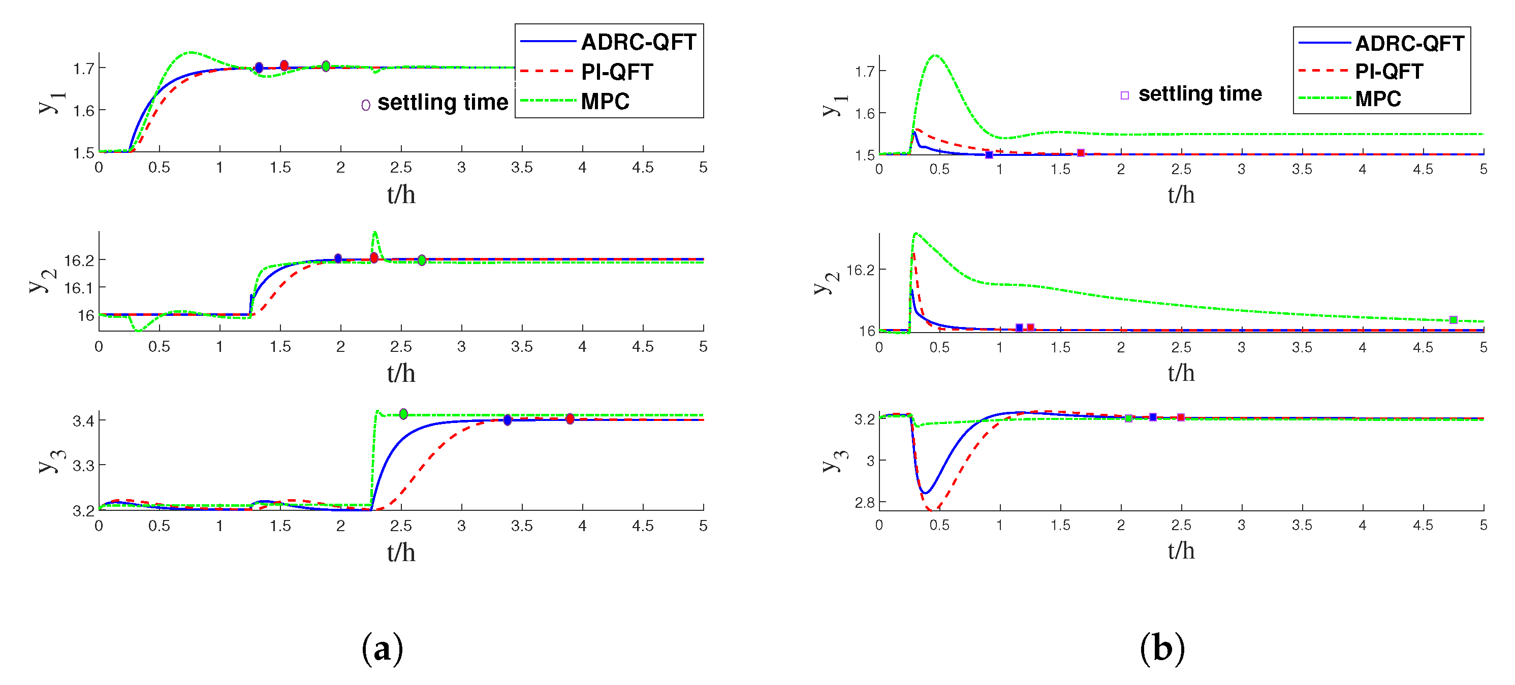
- The proposed method is applied to the toluene–methylcyclohexane extraction distillation process. Simulation experiments based on Aspen Dynamics and Matlab validate the proposed control method, demonstrating better tracking performance and disturbance rejection compared to traditional PI control and model predictive control.
2. Problem Formulation
3. Design of Disturbance Rejection Controller
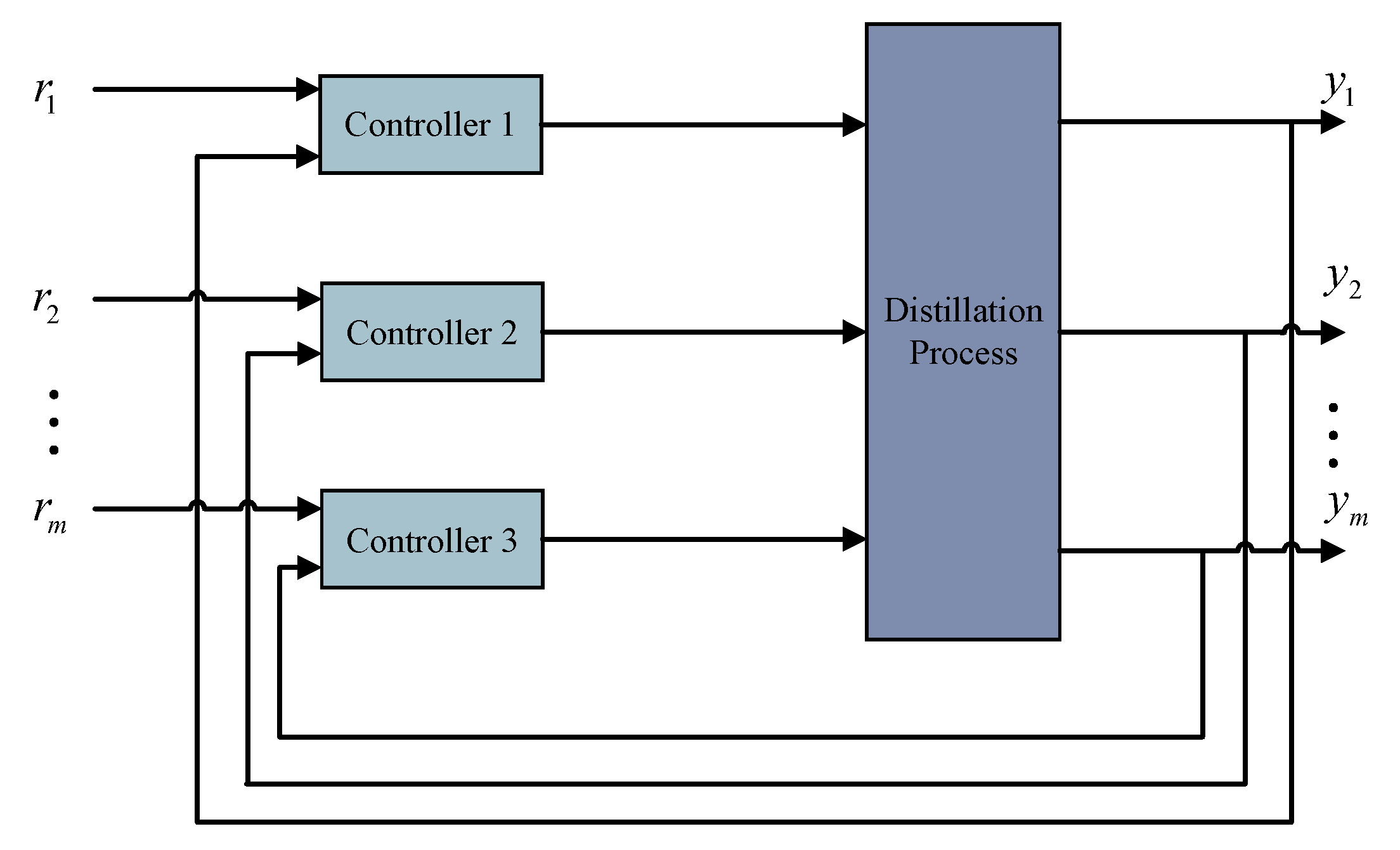
3.1. Multivariable Active Disturbance Rejection Control Structure
3.2. SISO Active Disturbance Rejection Controller Design
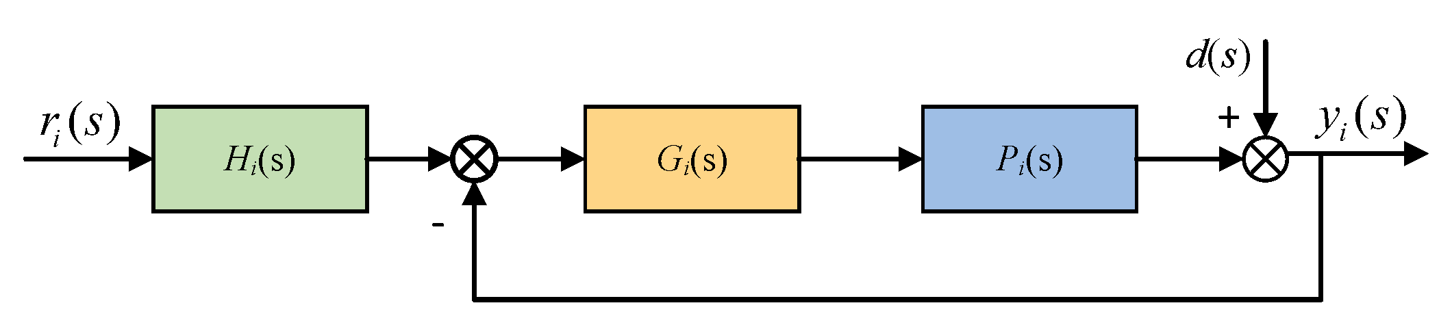
3.3. Equivalent Two-Degree-of-Freedom Control Structure
4. Optimal Design of Controller Based on Quantitative Feedback Theory
4.1. Quantitative Feedback Theory
4.1.1. Performance Specification in QFT
- (1)
- Robust stability performance specificationIn minimum-phase systems, the relative stability of the closed-loop system can be represented by the closed-loop resonant peak:where , represents the plant model under all uncertainty conditions, is the magnitude–frequency response curve of the closed-loop transfer function, and is the closed-loop resonant peak. The relationship between the system’s gain margin (), phase margin (), and is:
- (2)
- Disturbance rejection specificationThe disturbance rejection specifications for the system output and input are defined as and , respectively, as shown below:where and are designable parameters.
- (3)
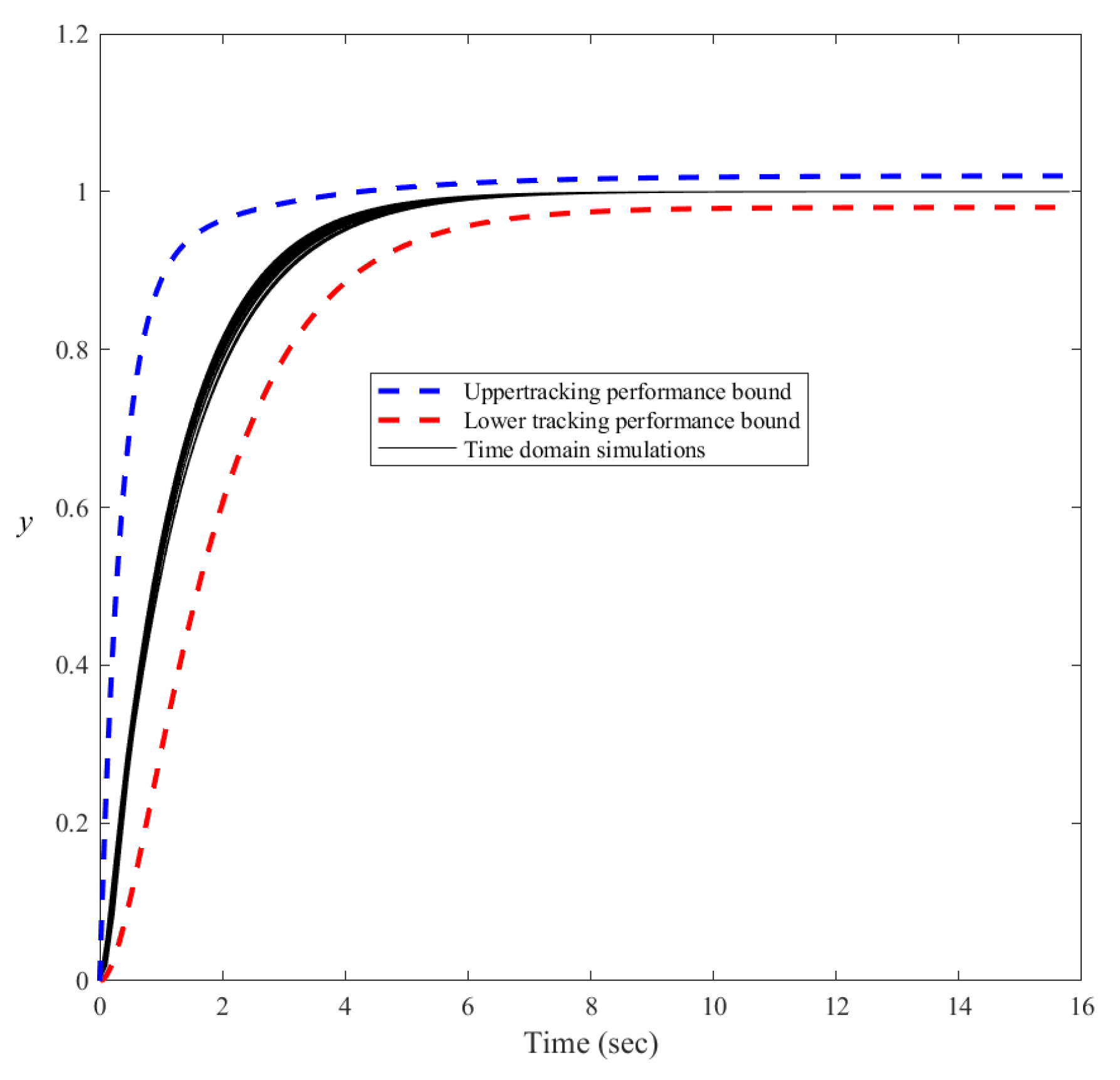
- Tracking performance specificationThe system tracking performance specification is designed as follows:where is the lower bound of the reference tracking performance specification, and is the upper bound. The parameters , , , , , , and are designable.
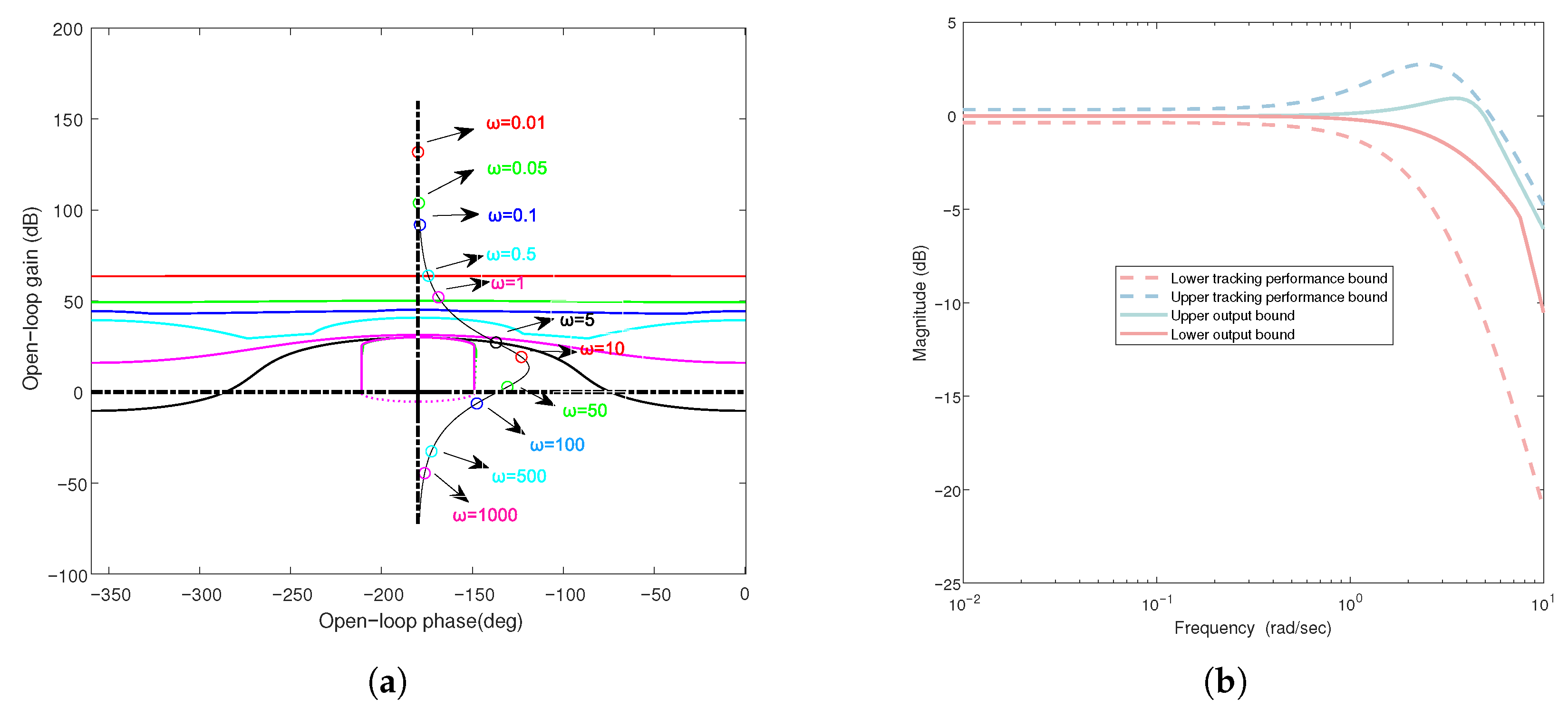
4.1.2. Loop Shaping
4.1.3. Prefilter Design and Validation
4.2. Parameter Optimization Based on QFT
- (1)
- In a reasonable loop shaping result, the system’s magnitude–frequency characteristic curve should change monotonically. This is verified by calculating the difference in magnitude characteristics across the frequency range and checking whether it changes monotonically.where denotes the magnitude of the system’s frequency response at that frequency point.
- (2)
- For the low-frequency range, the system’s open-loop frequency characteristics should correspond to points above the boundary curve for tracking and disturbance rejection synthesis, ensuring the system can accurately track the input signal and effectively reject disturbances.where represents the disturbance and tracking performance specifications of the system at frequency , and is the synthesized boundary for tracking and disturbance rejection performance.
- (3)
- For the high-frequency range, the system’s open-loop frequency characteristics should correspond to points outside the stability boundary curve, ensuring the system’s stability.where represents the robust stability index of the system at frequency (in the high-frequency range), and is the robust stability boundary.
4.3. Optimization Based on Improved Multi-Objective Grey Wolf Optimizer
Optimization Process of Improved MOGWO
- Initialize population and parameters:The initial positions of the grey wolf population vectors are generated through a Gaussian distribution-based initialization mechanism.where , with p being the population size; represents the midpoint of the lower and upper bounds of the search space; and denotes the standard deviation.
- Non-dominated sorting:Non-dominated sorting is performed on the initial solution set to generate different levels of non-dominated solution sets . Based on the sorting results, an archive population is established to store all non-dominated solutions.where k is the number of non-dominated solution sets.
- Dynamically adjust parameters based on the iteration count:As the number of iterations increases, the parameters a, A, and C are dynamically adjusted.where t is the current iteration number, is the maximum number of iterations, and represents a random number uniformly distributed in the range [0, 1].
- Grid-based leader selection mechanism:Based on fitness values and grid density, the alpha, beta, and delta wolves are selected, representing the best solution, the second-best solution, and the third-best solution, respectively.
- Update the positions of wolves in the population:The positions of the wolves in the population are updated based on the positions of the , , and wolves. The position update equations are as follows:where represents the position of the wolves at the t-th generation; , , and represent the positions of the , , and wolves, respectively; and are update parameters; and is the distance vector.
- Update the archive population:The fitness value of each individual is calculated, and the archive population is updated based on the fitness values.where is the fitness value vector of the -th individual, is the value of the -th objective function, and is the number of objective functions.
- Check the archive population:If the number of individuals in the archive population reaches the upper limit, the crowding distance is calculated and the individuals with higher crowding distances are removed to maintain the diversity of the solution set. The crowding distance calculation is:where is the crowding distance of the -th solution, and and are the values of the objective function of the adjacent individuals after sorting.
- Iteration:Check whether the maximum iteration number has been reached. If so, terminate the algorithm; otherwise, dynamically adjust parameters a, A, and C and continue iterating.
4.4. Optimization Result Selection
5. Simulation and Discussion
5.1. Numerical Simulation
- (1)
- Robust stability specification:where rad/s.
- (2)
- Output disturbance performance specification:where rad/s.
- (3)
- Input disturbance performance specification:where rad/s.
- (4)
- Reference tracking specification:where rad/s.
5.2. Application in Extraction Distillation Process
6. Conclusions
Author Contributions
Funding
Data Availability Statement
Acknowledgments
Conflicts of Interest
Abbreviations
| ADRC | Active disturbance rejection control |
| QFT | Quantitative feedback theory |
| MCH | Methylcyclohexane |
| PI | Proportional–integral |
| PID | Proportional–integral–derivative |
| MPC | Model predictive control |
| ESO | Extended state observer |
| MOGWO | Multi-objective gray wolf optimization algorithm |
| MIMO | Multiple-input multiple-output |
| SISO | Single-input single-output |
| 2DOF | Two-degree-of-freedom |
| GWO | Grey wolf optimizer |
| IAE | Integral absolute error |
References
- Halvorsen, I.J.; Skogestad, S. Energy efficient distillation. J. Nat. Gas Sci. Eng. 2011, 3, 571–580. [Google Scholar] [CrossRef]
- Jana, A.K. Heat integrated distillation operation. Appl. Energy 2010, 87, 1477–1494. [Google Scholar] [CrossRef]
- Mtogo, J.W.; Mugo, G.W.; Varbanov, P.S.; Szanyi, A.; Mizsey, P. Exploring Exergy Performance in Tetrahydrofuran/Water and Acetone/Chloroform Separations. Processes 2024, 12, 14. [Google Scholar] [CrossRef]
- Li, Q.; Wu, Q.; Zhao, S.; Pang, Y.; Yang, Z.; Hu, N. The Impact of Feed Composition on Entrainer Selection in the Extractive Distillation Process. Processes 2024, 12, 764. [Google Scholar] [CrossRef]
- Chernysheva, E.A.; Piskunov, I.V.; Kapustin, V.M. Enhancing the efficiency of refinery crude oil distillation process by optimized preliminary feedstock blending. Pet. Chem. 2020, 60, 1–15. [Google Scholar] [CrossRef]
- Shan, B.M.; Pang, Y.S.; Zheng, Q.; Xu, Q.L.; Wang, Y.L.; Zhu, Z.Y.; Zhang, F.K. Improved ANFIS combined with PID for extractive distillation process control of benzene-isopropanol-water mixtures. Chem. Eng. Sci. 2023, 74, 4945–4955. [Google Scholar] [CrossRef]
- Qian, X.; Dang, Q.; Jia, S.; Yuan, Y.; Huang, K.; Chen, H.; Zhang, L. Operation of distillation columns using model predictive control based on dynamic mode decomposition method. Ind. Eng. Chem. Res. 2023, 62, 21721–21739. [Google Scholar] [CrossRef]
- Han, J.Q. From PID to active disturbance rejection control. IEEE Trans. Ind. Electron. 2009, 56, 900–906. [Google Scholar] [CrossRef]
- Huang, Y.; Xue, W. Active disturbance rejection control: Methodology and theoretical analysis. ISA Trans. 2014, 53, 963–976. [Google Scholar] [CrossRef]
- Herbst, G. Practical Active Disturbance Rejection Control: Bumpless Transfer, Rate Limitation, and Incremental Algorithm. Comput. Sci. Inform. 2016, 63, 1754–1762. [Google Scholar] [CrossRef]
- Hou, G.; Huang, T.; Huang, C. Flexibility improvement of 1000 MW ultra-supercritical unit under full operating conditions by error-based ADRC and fast pigeon-inspired optimizer. Energy 2023, 270, 126852. [Google Scholar] [CrossRef]
- Sun, L.; Xue, W.; Li, D.; Su, Z. Quantitative tuning of active disturbance rejection controller for FOPTD model with application to power plant control. IEEE Trans. Ind. Electron. 2021, 69, 805–815. [Google Scholar] [CrossRef]
- Su, Z.; Sun, L.; Xue, W.; Lee, K. A review on active disturbance rejection control of power generation systems: Fundamentals, tunings and practices. Control Eng. Pract. 2023, 141, 105716. [Google Scholar] [CrossRef]
- Wu, Z.; Li, D.; Liu, Y.; Chen, Q. Performance analysis of improved ADRCs for a class of high-order processes with verification on main steam pressure control. IEEE Trans. Ind. Electron. 2023, 70, 6180–6190. [Google Scholar] [CrossRef]
- Ren, J.; Chen, Z.Q.; Sun, M.W.; Sun, Q.L.; Wang, Z.H. Proportion integral-type active disturbance rejection generalized predictive control for distillation process based on grey wolf optimization parameter tuning. Chin. J. Chem. Eng. 2023, 49, 234–244. [Google Scholar] [CrossRef]
- Mahapatro, S.R.; Subudhi, B. Disturbance rejection-based robust decentralized controller design for a multivariable system. Trans. Inst. Meas. Control 2021, 45, 620–636. [Google Scholar] [CrossRef]
- Horowitz, I. Survey of quantitative feedback theory (QFT). Int. J. Control 2001, 11, 887–921. [Google Scholar] [CrossRef]
- Houpis, C.H.; Rasmussen, S.J.; Garcia-Sanz, M. Quantitative Feedback Theory: Fundamentals and Applications; CRC Press: Boca Raton, FL, USA, 1999; pp. 15–32. [Google Scholar]
- Gu, D.W.; Petkov, P.; Konstantinov, M.M. Robust Control Design with MATLAB; Springer: London, UK, 2005; pp. 35–77. [Google Scholar]
- Pretorius, A.; Boje, E. A complementary quantitative feedback theory solution to the 2 × 2 tracking error problem. Int. J. Robust Nonlinear Control 2020, 30, 6569–6584. [Google Scholar] [CrossRef]
- Cheng, Y.; Fan, Y.; Zhang, P.; Yuan, Y.; Li, J. Design and parameter tuning of active disturbance rejection control for uncertain multivariable systems via quantitative feedback theory. ISA Trans. 2023, 141, 288–302. [Google Scholar] [CrossRef]
- Katal, N.; Narayan, S. Automated synthesis of multivariate QFT controller and pre-filter for a distillation column with multiple time delays. J. Process Control 2021, 99, 79–106. [Google Scholar] [CrossRef]
- Kobaku, T.; Poola, R.; Agarwal, V. Design of robust PID controller using PSO-based automated QFT for nonminimum phase boost converter. IEEE Trans. Circuits Syst. II Express Briefs 2022, 69, 4854–4858. [Google Scholar] [CrossRef]
- Fan, Y.L.; Cheng, Y.; Zhang, P.C.; Lu, G.P. An active disturbance rejection control design for the distillation process with input saturation via quantitative feedback theory. J. Process Control 2023, 128, 103029. [Google Scholar] [CrossRef]
- Baños, A.; Salt, J.; Casanova, V. A QFT approach to robust dual-rate control systems. Int. J. Robust Nonlinear Control 2022, 32, 1026–1054. [Google Scholar] [CrossRef]
- Garcia-sanz, M. Robust Control Engineering: Practical QFT Solutions; CRC Press: Boca Raton, FL, USA, 2017; pp. 17–78. [Google Scholar]
- Mirjalili, S.; Mirjalili, S.M.; Andrew, L. A Grey wolf optimizer. Adv. Eng. Softw. 2014, 69, 46–61. [Google Scholar] [CrossRef]
- Mirjalili, S.; Saremi, S.; Mirjalili, S.M.; Coelho, L. Multi-objective grey wolf optimizer: A novel algorithm for multi-criterion optimization. ISA Trans. 2016, 47, 106–119. [Google Scholar] [CrossRef]
- Luyben, W.L. Distillation Design and Control Using Aspen Simulation; John Wiley & Sons: New York, NY, USA, 2013; pp. 29–38. [Google Scholar]


| Symbol | Description | Operating Point |
|---|---|---|
| Number of trays | 22 | |
| Feed tray | 14 | |
| Distillate top pressure | 6 kPa | |
| Tray pressure drop | 0.68 kPa | |
| F | Feed flow rate | 1600 lbmol/hr |
| D | Distillate flow rate | 200 lbmol/hr |
| B | Bottom flow rate | 1400 lbmol/hr |
| R | Reflux ratio | 8 |
| MCH mass flow rate | 19,605 lb/hr | |
| Condenser medium flow rate | 180,250 lb/hr | |
| Bottom mass flow rate | 131,296 lb/hr | |
| Liquid level of tray 1 | 1.5 Ft | |
| Pressure of tray 1 | 16 psi | |
| Liquid level of tray 22 | 3.2 Ft | |
| Phenol feed temperature | 220 F |
| ADRC-QFT Parameters | |
|---|---|
| Loop 1 | |
| Loop 2 | |
| Loop 3 | |
| PI-QFT Parameters | |
| Loop 1 | |
| Loop 2 | |
| Loop 3 | |
| Control Strategy | Simulation Type | Loop 1 | Loop 2 | Loop 3 |
|---|---|---|---|---|
| ADRC-QFT | Tracking | 0.0406 * | 0.0274 * | 0.0487 * |
| Disturbance rejection | 0.0069 * | 0.0159 * | 0.1309 | |
| PI-QFT | Tracking | 0.0570 | 0.0581 | 0.1181 |
| Disturbance rejection | 0.0217 | 0.0222 | 0.2089 | |
| MPC | Tracking | 0.0562 | 0.0766 | 0.1489 |
| Disturbance rejection | 0.2956 | 0.4598 | 0.0376 * |
Disclaimer/Publisher’s Note: The statements, opinions and data contained in all publications are solely those of the individual author(s) and contributor(s) and not of MDPI and/or the editor(s). MDPI and/or the editor(s) disclaim responsibility for any injury to people or property resulting from any ideas, methods, instructions or products referred to in the content. |
© 2025 by the authors. Licensee MDPI, Basel, Switzerland. This article is an open access article distributed under the terms and conditions of the Creative Commons Attribution (CC BY) license (https://creativecommons.org/licenses/by/4.0/).
Share and Cite
Ye, Y.; Cheng, Y.; Zhou, F.; Lu, G. Optimization of Active Disturbance Rejection Controller for Distillation Process Based on Quantitative Feedback Theory. Processes 2025, 13, 1436. https://doi.org/10.3390/pr13051436
Ye Y, Cheng Y, Zhou F, Lu G. Optimization of Active Disturbance Rejection Controller for Distillation Process Based on Quantitative Feedback Theory. Processes. 2025; 13(5):1436. https://doi.org/10.3390/pr13051436
Chicago/Turabian StyleYe, Yinghao, Yun Cheng, Feng Zhou, and Guoping Lu. 2025. "Optimization of Active Disturbance Rejection Controller for Distillation Process Based on Quantitative Feedback Theory" Processes 13, no. 5: 1436. https://doi.org/10.3390/pr13051436
APA StyleYe, Y., Cheng, Y., Zhou, F., & Lu, G. (2025). Optimization of Active Disturbance Rejection Controller for Distillation Process Based on Quantitative Feedback Theory. Processes, 13(5), 1436. https://doi.org/10.3390/pr13051436