Theoretical Recommendations and Validation for the Generation of Realistic Irregular Waves Through the WaveMIMO Methodology

Abstract

Irregular wave generation in numerical simulations is critical for accurately modeling realistic sea conditions, which is essential in coastal and offshore engineering applications, such as for wave energy conversion. Therefore, this study presents theoretical recommendations for generating realistic irregular waves using the WaveMIMO methodology and validates its accuracy against experimental data. For the parameters investigation, spectral data are processed to obtain orbital velocity profiles of wave propagation, which are imposed as boundary conditions (BCs) in a numerical wave channel. The simulations were conducted using the ANSYS-Fluent 2024 R2 software, which employs the multiphase volume of fluid (VOF) model to treat the interface between phases. Seeking theoretical recommendations for the application of this methodology, the present study investigated the discretization of the region where the prescribed velocity BC is imposed, the mesh sensitivity in the free surface region, the time step used, and the location of the velocity vector in each segment of the prescribed velocity BC imposition region. The results obtained were compared with realistic sea state data obtained from the TOMAWAC spectral model, referring to the municipalities of Rio Grande and Tramandaí, in the state of Rio Grande do Sul, Brazil. The results indicated that, compared to recommendations from the previous literature, the recommended configuration improved wave generation accuracy by 7–8% for Rio Grande and 2–3% for Tramandaí. Finally, the WaveMIMO methodology and its theorical recommendations were validated against experimental data found in the literature, reaching an excellent agreement.

1. Introduction

The global energy sector is undergoing a critical transition as societies confront the dual challenges of climate change and the depletion of fossil fuel reserves. Growing environmental concerns about greenhouse gas emissions and ecological degradation, coupled with the finite nature of fossil resources, have driven nations to explore and integrate renewable alternatives into their energy matrices [1]. Among these, oceans represent an underexploited renewable resource, with wave energy standing out as particularly promising. Numerous global studies have assessed and quantified this potential across different countries, including Mexico [2], Algeria [3], France [4], Indonesia [5], India [6], Argentina, Brazil, Chile, Colombia, Uruguay [7], Australia [8], China [9], among others.

The energy contained in ocean waves can be extracted through converter devices that transform kinetic energy into electricity, such as oscillating water column (OWC), oscillating bodies, overtopping devices, and submerged horizontal plates (SHP) [10,11], along with other proposed technologies. These devices have been investigated through both experimental and numerical approaches. According to the International Energy Agency [12], beyond laboratory testing, multiple prototypes are currently under development or testing worldwide, including in China, South Korea, Singapore, Australia, New Zealand, the United States, Ireland, France, and Portugal.

Numerical modeling offers a cost-effective alternative for studying wave energy converters, requiring fewer financial and human resources. Consequently, numerous numerical studies have investigated the performance of wave energy conversion devices. Examples include OWC [13,14,15,16,17,18,19,20,21], overtopping [22,23,24,25,26,27,28,29,30], SHP [11,31,32,33], and even hybrid devices combining multiple conversion principles [34,35,36]. However, to enable reliable numerical investigations, it is crucial to accurately understand and reproduce wave behavior, particularly irregular waves, which represent real ocean conditions. Thus, developing robust numerical modeling methodologies for this phenomenon remains essential.

Numerical wave generation has evolved through diverse approaches, each addressing specific challenges in wave propagation modeling. For regular waves, conventional methodologies have been rigorously tested, such as Lisboa et al. [37], who performed numerical simulations using ANSYS-Fluent software to quantify the effects of linear and quadratic damping coefficients in numerical beaches, demonstrating significantly reduced wave reflection. Zabihi et al. [38] conducted a benchmark study between ANSYS-Fluent and Flow-3D, showing both models are powerful tools for wave generation. Windt et al. [39] presented a validation of a numerical wave tank model demonstrating strong agreement between simulated and experimentally monitored free surface elevations. Jiang et al. [40] studied regular wave propagation on a sloping bed under steady wind action, analyzing nearshore wave-wind interaction mechanisms; the results indicated that wind accelerates wave breaking, increases the breaker index, and enhances turbulence.

Regarding irregular wave generation, Oh et al. [41] developed a nonlinear wave simulation code using a higher-order spectral (HOS) method, employing fourth-order Runge–Kutta time integration and anti-aliasing zero-padding for stability; the results confirmed its efficiency in predicting nonlinear wave interactions. Choi et al. [42] presented a methodology for simulating nonlinear irregular waves using the HOS method, validated against extreme wave events; the results showed strong agreement between OpenFOAM, HOS, and experimental data in predicting wave breaking and elevations. Kim et al. [43] introduced a unified nonlinear wave generation and validation procedure for numerical and experimental wave tanks; a comparative analysis of mild and extreme breaking waves demonstrated strong agreement across stochastic and deterministic metrics between HOS simulations, OpenFOAM, and experimental results.

Moreover, Kim et al. [44] presented a real-time wave forecasting system for directional seas using Lagrangian-based models, enabling efficient processing of sparse optical measurement data; experimental validation confirmed that directional wave components must be considered to achieve accuracy comparable to unidirectional forecasts. Canard et al. [45] developed a wave generation method controlling both spectrum and crest statistics, enabling precise irregular wave field reproduction beyond spectral methods, particularly for unidirectional non-breaking conditions. Kim and Ducrozet [46] advanced the complementary improved choppy wave model (CICWM) to address directional wave field limitations by incorporating essential nonlinear terms. Experimental validation demonstrated CICWM reduces linear model prediction errors in directional seas while maintaining real-time forecasting capability through simplified assimilation.

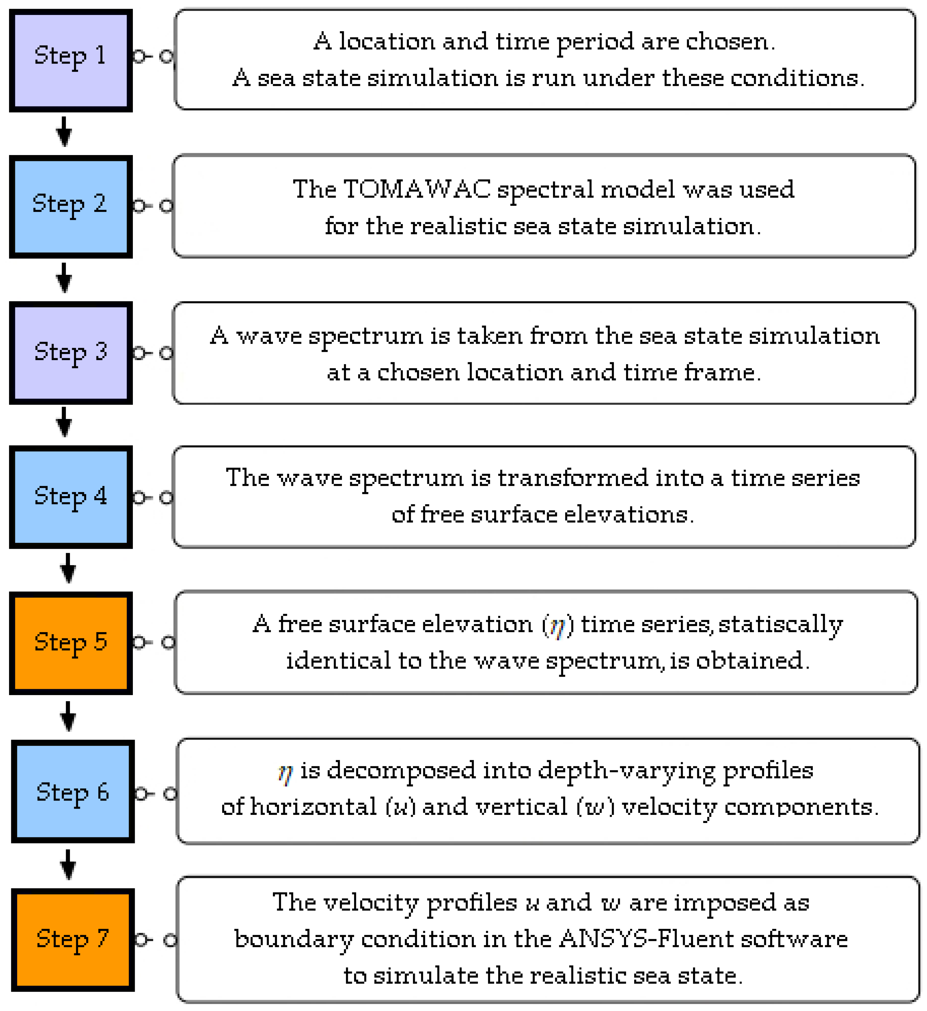
Another example is the WaveMIMO methodology, proposed and verified by Machado et al. [47], which is the focus of the present study. This methodology uses realistic sea state data to generate irregular waves, enabling reproduction of natural wave phenomena. To do so, spectral data are processed to obtain discretized wave propagation velocity profiles, imposed as prescribed velocity boundary conditions. Notably, the methodology’s capability for regular wave generation was validated by Maciel et al. [48] through numerical–experimental comparisons. Several studies have employed WaveMIMO to analyze wave energy converters fluid–dynamic behavior under realistic irregular waves, including geometric evaluations of the OWC [16,17], overtopping [25,30], and SHP [33] devices. Furthermore, specific aspects of the WaveMIMO methodology have been investigated in dedicated studies: Mocellin et al. [17] examined the influence of numerical wave channel bathymetry on realistic irregular wave generation, while Paiva et al. [49] and Maciel et al. [50] presented case studies evaluating key application parameters.

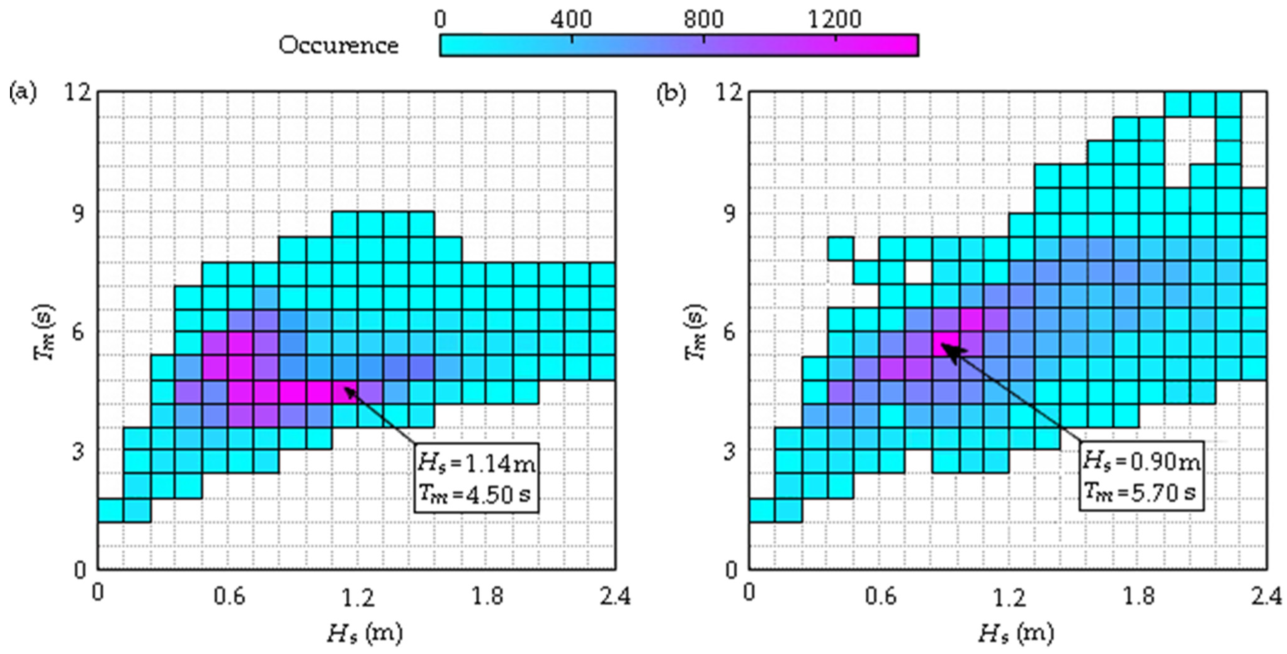
In this sense, the present study aims to establish general theoretical recommendations regarding the application of the WaveMIMO methodology [47]. The importance of refining the WaveMIMO methodology lies in its potential to generate realistic irregular waves, thereby achieving a more accurate representation of natural wave phenomena. Therefore, studies were carried out to simulate realistic irregular waves based on the sea states found on the coast of the Rio Grande do Sul (RS), southern Brazil. Locations with different characteristics of significant height, mean period, and water depth were analyzed, enabling an evaluation of the methodology’s performance under different wave climates. As a final contribution, this study validates the refined methodology by comparing numerical results with experimental data from the literature, a novel aspect of this paper.

2. Mathematical and Numerical Modeling

To carry out this study, numerical simulations of the generation and propagation of realistic irregular waves in a wave channel were conducted using the ANSYS-Fluent 2024 R2 software [51], based on the finite volume method (FVM). To treat the interface between the phases (water and air), the multiphase volume of fluid (VOF) [52] model was used. The representation of the phases in the computational model requires the concept of volumetric fraction (α), where the sum of the fractions in each control volume must be equal to 1. Thus, each computational cell can assume three distinct states, that is, containing only water, where [53]

$${\alpha }_{\mathrm{w}\mathrm{a}\mathrm{t}\mathrm{e}\mathrm{r}}=1,$$

(1)

containing only air, where [53]

$${\alpha }_{\mathrm{a}\mathrm{i}\mathrm{r}}=1,$$

(2)

or, containing the interface between both phases, which are immiscible fluids, where [53]

$${\alpha }_{\mathrm{w}\mathrm{a}\mathrm{t}\mathrm{e}\mathrm{r}}=1-{\alpha }_{\mathrm{a}\mathrm{i}\mathrm{r}}.$$

(3)

Furthermore, it is important to note that, when employing the VOF model, a single set of equations is solved, comprising the conservation equations for mass, volumetric fraction, and momentum. These equations are provided, respectively, by [54]

$${\displaystyle \frac{\partial \left(\rho \right)}{\partial t}}+\mathsf{\nabla }\left(\rho \overrightarrow{V}\right)=0,$$

(4)

$${\displaystyle \frac{\partial \left(\alpha \right)}{\partial t}}+\mathsf{\nabla }\left(\alpha \overrightarrow{V}\right)=0,$$

(5)

$${\displaystyle \frac{\partial }{\partial t}}\left(\rho \overrightarrow{V}\right)+\rho \left(\mathsf{\nabla }\overrightarrow{V}\right)\overrightarrow{V}=-\mathsf{\nabla }p+\mathsf{\nabla }\stackrel{=}{\tau }-\rho \overrightarrow{g}+S.$$

(6)

where $\rho$ is the fluid density (kg/m³), calculated for the mixture of phases as [53]

$$\rho ={\alpha }_{\mathrm{w}\mathrm{a}\mathrm{t}\mathrm{e}\mathrm{r}}{\rho }_{\mathrm{w}\mathrm{a}\mathrm{t}\mathrm{e}\mathrm{r}}+\left(1-{\alpha }_{\mathrm{w}\mathrm{a}\mathrm{t}\mathrm{e}\mathrm{r}}\right){\rho }_{\mathrm{a}\mathrm{i}\mathrm{r}},$$

(7)

while t is the time (s); $\overrightarrow{V}$ is the velocity vector (m/s); p is the static pressure (Pa); $\overrightarrow{g}$ is the gravity acceleration vector (m/s²); and $\stackrel{=}{\tau }$ is the strain rate tensor (N/m²). Additionally, it is important to note that the sink term (S) refers to the numerical beach tool, which applies damping to minimize reflections, and is given by [55,56]

$$S=-\left[C_1\mathsf{\rho }V+{\displaystyle \frac{1}{2}}{C}_2\mathsf{\rho }\left|V\right|V\right]\left(1-{\displaystyle \frac{z-z_{fs}}{z_b-z_{fs}}}\right){\left({\displaystyle \frac{x-x_s}{x_e-x_s}}\right)}^2,$$

(8)

where $C_1$ and $C_2$ are the linear (s⁻¹) and quadratic (m⁻¹) damping coefficients, respectively; $V$ is the velocity along the z direction (m/s); $z_{fs}$ and $z_b$ are the vertical positions of the free surface (FS) and the channel bottom (m); and $x_s$ and $x_e$ are the starting and ending positions of the numerical beach (m). Lastly, it is important to highlight that the damping coefficients, $C_1$ and $C_2$, are set to $20$ s⁻¹ and $0$ m⁻¹, respectively, as recommended by [37].

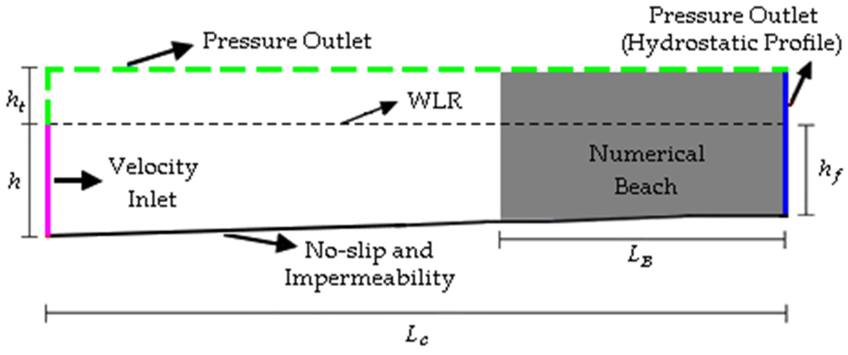
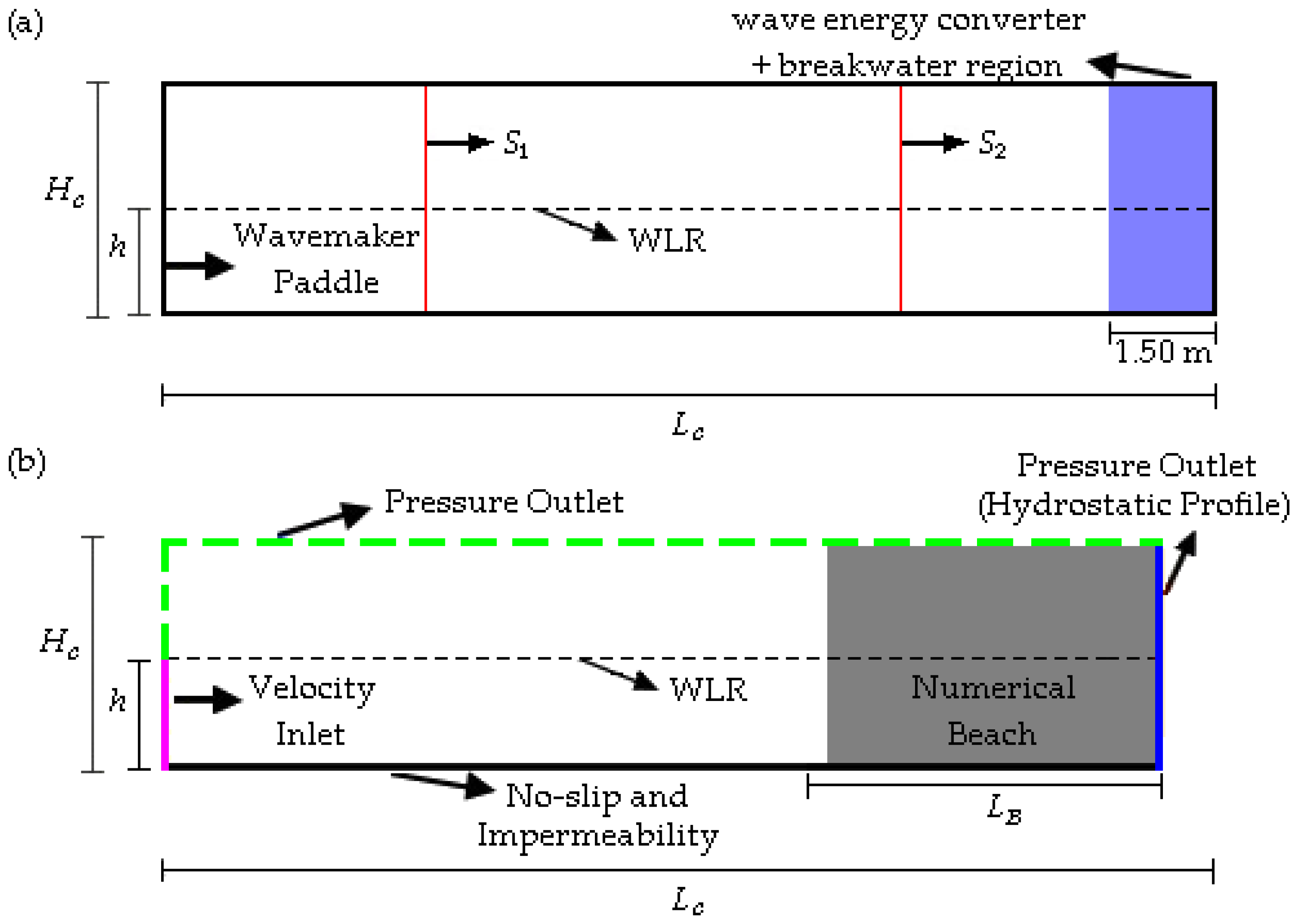
In addition to the governing equations, the following boundary conditions (detailed later in Section 4.1) were applied to model the numerical wave channel:

• Prescribed velocity: where discretized orbital velocity profiles are imposed (WaveMIMO methodology);
• Pressure outlet: atmospheric pressure was considered, i.e., $p=101.30$ kPa;
• No-slip and impermeability: where null velocities were considered, $\overrightarrow{V}=0$ m/s.

Numerical Methods Applied

To conduct numerical simulations in the ANSYS-Fluent software, specific set of configurations were defined to solve the governing equations of the problem. The pressure-implicit with splitting of operators (PISO) scheme employed for the pressure–velocity coupling, while the pressure staggering option (PRESTO) scheme was used for pressure spatial discretization. These approaches are summarized in

Table 1. Methods and parameters used in the present numerical simulations.

Parameters		Numerical Inputs
Solver		Pressure-Based
Pressure–Velocity Coupling		PISO
Spatial Discretization	Gradient Evaluation	Green-Gauss-Cell-Based
	Pressure	PRESTO
	Momentum	First Order Upwind
	Volume Fraction	Geo-Reconstruct
Temporal Differencing Scheme		First Order Implicit
Under-Relaxation Factors	Pressure	0.3
	Momentum	0.7
Residual	Continuity	10−3
	x-velocity
	z-velocity
Regime Flow		Laminar

, along with other numerical methods used in this study.

It is highlighted that the flow was considered under a laminar regime, which, according to Gomes et al. [57], is a simplification that does not cause significant accuracy loss while reducing computational processing time. The simulation was initialized with inertia-dominated flow conditions. Additionally, the numerical procedures adopted were adapted from methodologies established in previous studies, such as those by [17,47,48,49].

3. WaveMIMO Methodology

In general, the WaveMIMO methodology involves numerically generating waves by imposing discretized wave propagation velocity profiles in the horizontal ($u$) and vertical ($w$) directions as prescribed velocity boundary conditions (BC). To do so, the Spec2Wave 1.2.1 software [58] is used to process realistic sea state data to obtain these velocity profiles. A flowchart of the WaveMIMO methodology is presented in Figure 1. It should be noted that the purple boxes indicate the user inputs (location/time selection); the blue boxes are the software processing steps (TOMAWAC, Spec2Wave); and the orange boxes are the WaveMIMO methodology’s outputs (free surface elevation time series, velocity profiles).

3.1. Realistic Sea State Data

As illustrated in Figure 1, Step 1 for applying the WaveMIMO methodology involves defining a location and a time interval. For the studies conducted in this paper, a realistic sea state database for the coast of RS, Brazil, for the year 2018 was used. This database was generated using the TOMAWAC spectral model (Step 2). This model obtains data by solving the equation that describes the general behavior of wave propagation in an unstable and inhomogeneous medium, as given by [59]

$${\displaystyle \frac{\partial N}{\partial t}}+{\displaystyle \frac{\partial \left(\dot{x}N\right)}{\partial x}}+{\displaystyle \frac{\partial \left(\dot{z}N\right)}{\partial z}}+{\displaystyle \frac{\partial \left({\dot{k}}_{x}N\right)}{\partial k_x}}+{\displaystyle \frac{\partial \left({\dot{k}}_{z}N\right)}{\partial k_z}}=Q\left(k_x,k_z,x,z,t\right),$$

(9)

where N represents the directional spectrum of wave action density (m²/Hz/rad); $k_x$ the component x of the wave number vector (m⁻¹); $k_z$ the component z of the wave number vector (m⁻¹). Moreover, Q is the source term (m²/rad), which aggregates standard spectral wave processes, such as wind input, dissipation mechanisms, and nonlinear interactions. Details regarding its complete mathematical formulations can be found in the model’s technical documentation [59].

The realistic sea state generated is then characterized by statistical parameters, such as the mean period ($T_m$) of the irregular waves. This parameter is essentially an arithmetic average of the wave periods within the spectrum, weighted by their contribution to the spectral energy [59]. The other is the significant wave height ($H_s$), which is widely used to describe sea states, as it represents the waves responsible for the most significant surface agitation [60].

Thus, each point in the domain contains statistical data on the observed $H_s$ and $T_m$, which are analyzed to determine the most frequent sea state at each study site. In this investigation, it was considered realistic sea states from the municipalities of Rio Grande and Tramandaí, located in the southern and northern regions of the RS coast, respectively. Figure 2 presents the bivariate histogram that relates the occurrences of $H_s$ and $T_m$ and identifies the most frequent combination for the municipalities of (a) Rio Grande and (b) Tramandaí. It allows for the wave spectrum taken from the simulation (Step 3) to be determined.

Through these statistical parameters, along with the depth ($h$) found in each location, it is possible to establish the representative regular waves for the sea states addressed. The final characteristic to be determined is the wavelength, which is calculated using the dispersion equation [61]:

$${\omega }^2=gk\mathit{tanh}\left(kh\right),$$

(10)

where $\omega$ is the angular frequency (Hz); while $k$ is the wave number (m⁻¹), given, respectively, by the following [61]:

$$\omega ={\displaystyle \frac{2\pi }{T}},$$

(11)

$$k={\displaystyle \frac{2\pi }{\lambda }},$$

(12)

with $\lambda$ being the wavelength (m); and $T$ the wave period (s).

Thus, the characteristics of the representative regular waves are presented in

Table 2. Characteristics of representative regular waves of each sea state addressed.

Municipality	$\mathbf{Height}—\mathit{H}$ (m)	$\mathbf{Length}—\mathit{\lambda }$ (m)	$\mathbf{Period}—\mathit{T}$ (s)	Depth—h (m)
Rio Grande	1.14	31.50	4.50	13.29
Tramandaí	0.90	45.91	5.70	10.98

, where $H$ and $T$ stand, respectively, for $H_s$ and $T_m$ (see Figure 2). One can note that these wave characteristics are similar to those found in China [9] and Spain [62], for example. In this study, these characteristics are used as reference parameters for both the spatial and temporal discretization of the computational domain as in [17,30,47,49].

Next, the database is searched for FS elevation time series corresponding to the most frequent combinations of $H_s$ and $T_m$ at each location. These time series are then reproduced in the ANSYS-Fluent software using the WaveMIMO methodology.

Table 3. Characteristics of the selected locations and time periods for the studies.

Municipality	Geographic Coordinate	Shore Distance (m)	Date	Time
Rio Grande	32°11′24″ S, 52°04′45″ W	171.06	9 November 2018	07:15
Tramandaí	29°59′51″ S, 50°06′18″ W	2094.33	28 May 2018	10:15

provides detailed information on the selected locations, as well as the time period to which the data correspond. It should be noted that, in the case of Rio Grande, the distance shown in Table 3 refers to the distance to the local breakwater.

3.2. Obtaining Discretized Orbital Velocity Profiles

Following the flowchart presented in Figure 1, the next step involves transforming the wave spectrum into a time series of the corresponding FS elevation (Step 4). This is achieved using the Spec2Wave software [63], based on the methodology described in Oleinik et al. [63], which applies the Inverse Fourier Transform to the selected spectrum. Once the time series of the FS elevation for realistic irregular waves is obtained, it can be approximated by a finite sum of monochromatic waves (Step 5). These waves are individually described, according to Airy’s Linear Wave Theory, by [61]

$$\eta =A\mathit{cos}\left(kx-\omega t\right),$$

(13)

while the velocity potential is given by [60]

$$\varphi =-A{\displaystyle \frac{g}{\omega }}{\displaystyle \frac{cosh\left(kh+kz\right)}{cosh\left(kh\right)}}sin(kx-\omega t)$$

(14)

Thus, the orbital velocity profiles of wave propagation can be obtained (Step 6). These profiles come from the partial derivatives in the horizontal ($u$) and vertical ($w$) directions, and are given, respectively, by [61]

$$u=\omega A{\displaystyle \frac{\mathit{cosh}\left(kz+kh\right)}{\mathit{sinh}\left(kh\right)}}\mathit{cos}\left(kx-\omega t\right),$$

(15)

$$w=\omega A{\displaystyle \frac{\mathit{sinh}\left(kz+kh\right)}{\mathit{sinh}\left(kh\right)}}\mathit{sin}\left(kx-\omega t\right),$$

(16)

where $A$ is the wave amplitude (m), given by [61]

$$A={\displaystyle \frac{H}{2}}.$$

(17)

Therefore, it is obtained the discrete data that constitute the orbital velocity profiles, which are later used as BC in the ANSYS-Fluent software (Step 7). It allows to reproduce the FS elevation data of realistic irregular waves of a given region and period of time. Moreover, it is worth noting that when a series of FS elevation data are available, the WaveMIMO methodology can be applied to extract the $u$ and $w$ velocity profiles directly from it, skipping Steps 1–5 (see Figure 1).

4. Description of Case Studies

4.1. Parameter Evaluation Studies

A series of four sequential studies on the generation of realistic irregular waves was conducted, with each subsequent study building upon the findings of its predecessor. Thus, investigations were carried out regarding the discretization of the prescribed velocity BC imposition region, mesh sensitivity in the FS region, time step independence, and velocity vector location. It is worth noting that these studies were also performed considering the realistic sea state found in the Mostardas (MS) municipality, referring to the location of geographic coordinates 31°09′51″ S, 50°47′27″ W [49].

To this end, it was necessary to develop two distinct computational domains for the wave channels, one for each municipality considered. This approach was necessary because the channel dimensions depend on the characteristics of the regular waves that represent the realistic sea states addressed. Figure 3 illustrates the computational domain that should be adapted for Rio Grande and Tramandaí, highlighting the principal quotas, the BC implemented, the region where the numerical beach is imposed, and the water level at rest (WLR).

As observed in Figure 3, at the bottom of the channel (black solid line), the non-slip and impermeability BC is applied where the velocities $u$ and $w$ are considered null. On the lower portion of the left wall (pink solid line), the prescribed velocity BC is imposed. On the upper portion of the left wall and at the top of the channel (green dashed line), atmospheric pressure is applied. Notably, the atmospheric pressure BC is also used on the right lateral wall (blue solid line) to characterize an open flow channel. Additionally, a hydrostatic profile is imposed to ensure that the mean water level remains at a constant depth equal to $h_f$, preventing the wave channel from emptying.

Moreover, as also illustrated in Figure 3, the channel depth varies to replicate the bathymetry observed at the study site, as indicated by Mocellin et al. [17]. To achieve this, bathymetric data from nautical charts provided by the Brazilian Navy’s Hydrography and Navigation Directorate [64] were utilized. According to the recommendations of Lisboa et al. [37], the region where the numerical beach is imposed extends over a length of $2\lambda$. It is also worth mentioning that, in both cases, the top of the channel is positioned $5.00$ m above the WLR, corresponding to $h_t=5.00$ m. The remaining dimensions for each wave channel are detailed in

Table 4. Characteristics of the numerical wave channels employed.

Municipality	$\mathit{h}$ (m)	${\mathit{h}}_{\mathit{f}}$ (m)	${\mathit{L}}_{\mathit{C}}$ (m)	${\mathit{L}}_{\mathit{B}}$ (m)
Rio Grande	13.29	10.54	171.06	63.00
Tramandaí	10.98	10.59	229.56	91.82

.

For the spatial discretization of the computational domain, the stretched mesh [56] was adopted, featuring increased refinement in the region of interest, specifically the FS region. Thus, the computational domain was divided vertically into three regions. The first region, R1, contains only air and demands less refinement; it was discretized into 20 computational cells. The second one is the FS region, R2, containing the water–air interface, which requires greater refinement to ensure numerical convergence; it was discretized into 40 cells. The last vertical region is R3, containing only water. Since phenomena in this region influence the problem more substantially than those in R1, it was discretized into 60 computational cells. Moreover, horizontally, only one region is considered, R4, where 50 computational cells were allocated per $\lambda$. Figure 4 illustrates the stretched mesh.

Figure 4 also illustrates the lines $r_a$ and $r_b$, which represent the upper and lower limits of the FS region in the stretched mesh, respectively. Additionally, for temporal discretization, an initial time step of $\mathsf{\Delta }t=0.05$ s was used, following the recommendation of Machado et al. [47], for a total simulation time of 900 s of generation and propagation of realistic irregular waves, $\lambda$.

Aiming to analyze the results obtained, a probe was used to monitor the elevation of the FS in the wave generation zone, specifically at $x=0$ m. These results were compared with the FS elevation derived from the TOMAWAC spectral model. To quantitatively evaluate the results, the metrics mean absolute error (MAE) and root mean square error (RMSE) were considered [65]. However, it is important to note that differently scaled data produce differently scaled metric values. Thus, the metrics were normalized following the approach adopted in [39,48,66,67]. Thus, the normalized metrics, NMAE and NRMSE, are given, respectively, as follows:

$$\mathrm{N}\mathrm{M}\mathrm{A}\mathrm{E}=\left({\displaystyle \frac{1}{\mathrm{M}}}{\sum }_{i=1}^M{O}_i-P_i\right){\displaystyle \frac{100}{P_{max}-P_{min}}},$$

(18)

$$\mathrm{N}\mathrm{R}\mathrm{M}\mathrm{S}\mathrm{E}=\left(\sqrt{{\displaystyle \frac{1}{M}}{\sum }_{i=1}^M{\left(O_i-P_i\right)}^2}\right){\displaystyle \frac{100}{P_{max}-P_{min}}},$$

(19)

where $O_i$ represents the value obtained from ANSYS-Fluent (m); $P_i$ represents the data derived from TOMAWAC (m), with $P_{max}$ and $P_{min}$ being the maximum and minimum values found, respectively; and $M$ denotes the total amount of data.

4.1.1. Prescribed Velocity Boundary Condition Imposition Region—Description

The objective here is to investigate the discretization of the numerical wave channel region where the prescribed velocity BC is applied. For the implementation of the WaveMIMO methodology, it is necessary to subdivide this region into segments, where the transient discrete data of the orbital wave propagation velocities are inserted. In this context, it is worth mentioning that the subdivision recommended by Machado et al. [47] is $h/14$, meaning the depth of the location is divided into 14 equal segments, as illustrated in Figure 5, where the segments are represented by the colors blue and pink.

In addition to the aforementioned approach, two other analyses were proposed, which involve relating $h$ to the parameters of maximum wave amplitude ($A_{max}$) and significant wave height ($H_s$) of the realistic irregular waves. Thus, instead of fixing the number or size of the segments to be used, this approach varies according to the elevation series under consideration, with segments approximately equal in size to $A_{max}$ or $H_s$. It should be noted that $A_{max}$ is determined by the magnitude of the highest crest or the deepest trough found in the FS elevation series. In this context,

Table 5. Characteristics of the cases evaluated for the study of the discretization in the region of the prescribed velocity BC considering the realistic sea state found in Rio Grande.

Case	Parameter	Number of Segments	Segment Dimension (m)
1	$h/14$	14	0.95
2	$H_s$	11	1.21
3	$A_{max}$	8	1.66

and

Table 6. Characteristics of the cases evaluated for the study of the discretization in the region of the prescribed velocity BC considering the realistic sea state found in Tramandaí.

Case	Parameter	Number of Segments	Segment Dimension (m)
1	$h/14$	14	0.78
2	$H_s$	12	0.92
3	$A_{max}$	9	1.22

present the characteristics of each case evaluated, respectively, for Rio Grande and Tramandaí.

One can note that the FS region size differs for each case analyzed, and each computational domain. This variation arises because this region is determined by the size of the segments used, incorporating one segment above and another below the WLR. Furthermore, the discretization of 40 computational cells vertically within the FS region was maintained for all cases analyzed.

4.1.2. Mesh Sensitivity—Description

After determining the best approach for the discretization of the region where the prescribed velocity BC is applied, a mesh sensitivity analysis was performed regarding the FS region. This study was inspired by the recommendation of Romanowski et al. [68], which suggests that the FS region should be subdivided into distinct areas, i.e., the most refined regions are those that contain the majority of the elevations, which requires a statistical analysis.

In addition to the approach adopted in the previous study (Section 4.1), which follows the recommendation of Gomes et al. [57], this study proposes evaluating three additional discretization approaches that do not require statistical analysis of the elevations of the realistic irregular waves to be numerically reproduced. The proposed new approaches involve dividing each segment of the FS region into two equal-sized segments and varying the number of computational cells applied to each one, as illustrated in Figure 6. The lines $r_a$ and $r_b$ shown in Figure 6 represent, respectively, the upper and lower bounds of the R2 domain region (see Figure 4).

Thus, the analyzed cases were as follows:

• Case 4: each segment was discretized into 10 cells, totaling 40 computational cells vertically, maintaining the refinement suggested by Gomes et al. [57];
• Case 5: the central segments (around the WLR) were discretized into 20 cells, while the remaining segments were discretized into 10, totaling 60 computational cells vertically. This approach resembles the recommendation by Romanowski et al. [68];
• Case 6: Each segment was discretized into 20 cells, doubling the refinement suggested by Gomes et al. [57], resulting in 80 computational cells vertically.

4.1.3. Time Step Independence—Description

After defining the spatial discretization aspects to be applied, a temporal discretization investigation was conducted. In this regard, a time step independence study was performed to establish a relationship between the time step ($\mathsf{\Delta }t$) and $T_m$. The aim was to identify the relationship that provides the best match between the FS elevations generated in ANSYS-Fluent and those obtained through the TOMAWAC spectral model. The evaluated cases for both wave climates considered are presented in

Table 7. Cases tested for the time step independence study.

Case	Ratio	$\mathsf{\Delta }\mathit{t}$ (s)—Rio Grande	$\mathsf{\Delta }\mathit{t}$ (s)—Tramandaí
7	$T_m/60$	0.0750	0.0950
8	$T_m/90$	0.0500	0.0630
9	$T_m/120$	0.0375	0.0475
10	$T_m/150$	0.0300	0.0380

.

4.1.4. Location of the Velocity Vector—Description

The final investigation proposed concerns the location of the velocity vector that contains transient discrete data forming the orbital velocity profiles of wave propagation used as a prescribed velocity BC. It is important to note that the calculation of u and w profiles is performed within the Spec2Wave software, where their positions (vertical coordinates) are indicated, ranging from $0$ to $h$.

Following the recommendation of Machado et al. [47], the velocity vector is positioned at the center of each segment in the BC imposition region. In addition to this approach, two other methods were evaluated, as illustrated in Figure 7. These were proposed by Maciel et al. [50] in a study conducted considering the sea state for the municipality of Rio Grande in 2014. The present study aimed to identify which approach provides the best results, as follows:

• Case 11: positioning the vector at the upper part of the segments;
• Case 12: positioning the vector at the center of the segments;
• Case 13: positioning the vector at the lower part of the segments.

4.2. WaveMIMO Methodology Validation

The final study aims to validate the numerical model and the theoretical recommendations for the WaveMIMO methodology. For this purpose, a numerical simulation was conducted using a two-dimensional domain at laboratory scale, replicating the experiment by Koutrouveli et al. [34]. It is important to highlight that, in previous studies (Section 4.1), spectral data were processed to obtain a time series of FS elevations. In the present study, however, the FS elevation data monitored by probe $S_1$ in [34] were used. Thus, Steps 1–5 for applying the WaveMIMO methodology were skipped (see Figure 1).

As previously mentioned, these data were processed using the Spec2Wave software to obtain the discretized orbital velocity profiles, which were imposed as prescribed velocity BCs. Consequently, in the present study, the wave generation zone ($x=0$ m) was aligned with the position of probe $S_1$ in the experiment by Koutrouveli et al. [34]. Figure 8a presents the illustration of the physical setup used in the laboratory experiment of Koutrouveli et al. [34], while Figure 8b presents the computational domain used for model validation, highlighting the main dimensions and the BC applied.

In the laboratory experiment of Koutrouveli et al. [34] (Figure 8a), the wave channel had height of $H_C=1.20$ m and a total length of $L_C=14.00$ m, with the first 12.50 m dedicated to free wave propagation, while the last 1.50 m included a breakwater with a wave energy converter device attached. Two probes were used to monitor the FS elevation: the first, ($S_1$), positioned at $x=3.80$ m and the second, ($S_2$), at $x=9.50$ m, i.e., 5.70 m away from the first probe. By replicating this setup, the WaveMIMO methodology can be validated for both irregular wave generation and propagation. Thus, irregular waves were generated with the following characteristics: $H_s=0.034$ m, peak period, $T_p=1.27$ s, $\lambda =2.20$ m, and channel depth, $h=0.488$ m.

Due to the lack of detailed information regarding all physical characteristics of the laboratory experiment [34], certain adaptations were required. To maintain consistency with the computational model applied in previous studies, the numerical wave channel employed in the present study (Figure 8b) was defined with a height $H_C=1.20$ m and a length $L_C=13.10$ m. This length corresponds to the 12.50 m free wave propagation region in [34], excluding the initial 3.80 m (alignment with $S_1$) and including an additional 4.40 m numerical beach, following the $2\lambda$ recommendation Lisboa et al. [37]. Notably, the numerical beach was incorporated in the physical-to-numerical model adaptation because the experimental wave channel featured a dynamic reflection absorption system integrated in the wavemaker. Additionally, the physical setup had breakwaters on both sides of the hybrid wave energy converter device, enhancing wave energy dissipation toward the channel’s end. According to Koutrouveli et al. [34], coupling the device with the breakwater even improved its hydraulic performance.

As in previous studies performed here, the spatial and temporal discretization of the computational domain was based on the characteristics of the generated waves. Additionally, the numerical configurations employed were maintained, as well as the theoretical recommendations obtained for the application of the WaveMIMO methodology. Thus, two probes were used to monitor the FS elevation: the first, positioned in the generation zone, at $x=0$ m and the second, in the propagation zone, at $x=5.70$ m, corresponding to $S_2$ in [34]. The results were compared with the experimental and numerical data presented by Koutrouveli et al. [34]. As before, the quantitative evaluation was carried out using the NMAE and NRMSE metrics.

5. Results

5.1. Parameter Evaluation Studies

This section presents the results obtained throughout the investigations into the WaveMIMO methodology parameters and their respective discussions. It is worth mentioning that the studies were conducted sequentially, meaning the findings from each preceding investigation provided support the execution of the subsequent one.

For the analysis of these results, the findings from Paiva et al. [49] were incorporated to the discussions, as the authors evaluated the same WaveMIMO methodology parameters using data from the municipality of Mostardas, in the central region of the RS state coast, Brazil. The integration of these findings strengthens the generalizability of the parameter evaluations, since it provides a geographical complementarity to the municipalities addressed in the present study (Rio Grande in the south and Tramandaí in north of the RS state). Additionally, it is worth noting that the aforementioned article was authored by the same researchers involved in the current study, ensuring that the same numerical model was implemented.

5.1.1. Prescribed Velocity Boundary Condition Imposition Region—Results

To enable a better analysis during the evaluation of the results, the qualitative comparison of the FS elevation ($\eta$) was divided into three time-intervals, each spanning 300 s. Furthermore, the plotted graphs feature lines parallel to the x-axis, outlining the FS region (see Figure 6). Each pair of lines corresponds to an evaluated case, as follows:

• $r_{1a}$ and $r_{1b}$: solid lines, corresponding to Case 1;
• $r_{2a}$ and $r_{2b}$: dashed lines, corresponding to Case 2;
• $r_{3a}$ and $r_{3b}$: dotted lines, corresponding to Case 3.

It should be noted that the position of these lines on the z-axis relates to the size of the segments considered in each case (see Table 5 and Table 6). Thus, Figure 9 presents the monitored results for the realistic sea state observed in Rio Grande. As shown, in all cases, the realistic irregular waves generated through the WaveMIMO Methodology accurately reproduce the realistic sea state derived from TOMAWAC. Additionally, one can note the absence of initial inertia conditions effects, which is due to the fact that the results were monitored at $x=0$ m.

In cases where the segments used for discretizing the prescribed velocity BC imposition region are smaller than the $A_{max}$ parameter (Case 3), wave crests and troughs extend outside the FS region, as observed in [49]. It is possible to see time instants where the crests and troughs cross the $r_{1a}$ and $r_{1b}$ lines in Figure 9a, near $t=0$ s, in Figure 9b, around $t=450$ s and $t=600$ s, and Figure 9c, near $t=650$ s. On the other hand, the only occurrence where the $r_{2a}$ and $r_{2b}$ lines were also crossed happen in Figure 9a, near $t=0$ s. Notably, the $r_{3a}$ and $r_{3b}$ lines are never reached, as the trough used to define $A_{max}$, which occurs close to $t=0$ s, was not reached by the realistic irregular waves generated though the WaveMIMO methodology.

Therefore, most generated elevations remain within the region bounded by lines $r_{1a}$ and $r_{1b}$, which contain computational cells of practically identical size. For proper evaluation of these results, quantitative analysis is required.

Table 8. Quantitative results for the discretization study of the prescribed velocity BC imposition region, evaluated under Rio Grande’s realistic sea state.

Case	$\mathsf{\Delta }\mathit{z}$ (m)	NMAE (%)	NRMSE (%)	Processing Time (h)
1	0.0237	3.7303	4.8421	5.92
2	0.0302	3.7730	4.9046	5.72
3	0.0415	3.8388	4.9934	5.67

summarizes the NMAE and NRMSE metrics, along with the vertical dimension ($\mathsf{\Delta }z$) of each mesh element within the FS region and the respective processing times for all cases.

As shown in Table 8, NMAE and NRMSE values reveal a consistent but gradual degradation in accuracy as the size of the segments increased. Thus, Case 1 emerges as the best-performing scenario, since it presented the lowest NMAE and NRMSE values. While the absolute differences in metrics across cases appear small, the relative degradation in accuracy is notable. Compared to Case 1, Case 2 shows increases of 1.10% (NMAE) and 1.30% (NMRSE), while Case 3, the worst-performing scenario, exhibits larger increases of 2.90% (NMAE) and 3.10% (NRMSE). In comparison to Case 1, it was noted that Case 2 has elements 27.43% larger and a processing time 3.38% shorter, whereas Case 3 has elements 75.11% larger and a processing time 4.22% shorter.

Following the same methodology applied to Rio Grande, a qualitative assessment was conducted for the results obtained considering the realistic sea state found in the municipality of Tramandaí. Thus, Figure 10 compares the FS elevation monitored against the TOMAWAC data, demonstrating that in all cases, the realistic irregular waves generated using the WaveMIMO methodology accurately replicate the sea state addressed. Moreover, no inertia conditions effects are noted since results were monitored at $x=0$ m.

As before, there are time instants where wave crests and troughs cross the $r_{1a}$ and $r_{1b}$ lines, such as in Figure 10a, near $t=70$ s and $t=250$ s, Figure 10b, around $t=550$ s, Figure 10c, close to $t=600$ s. Additionally, troughs are observed to cross the $r_{2a}$ and $r_{2b}$ lines in Figure 10c, near $t=600$ s. As previously noted for the realistic sea state of Rio Grande, the $r_{3a}$ and $r_{3b}$ lines are never reached, since the crest used to define $A_{max}$ was not attained by the realistic irregular waves generated through the WaveMIMO methodology.

Consequently, most elevations remain within the region bounded by the $r_{1a}$ and $r_{1b}$ lines.

Table 9. Quantitative results for the discretization study of the prescribed velocity BC imposition region, evaluated under Tramandaí’s realistic sea state.

Case	$\mathsf{\Delta }\mathit{z}$ (m)	NMAE (%)	NRMSE (%)	Processing Time (h)
1	0.0392	4.4364	5.5955	6.03
2	0.0450	4.4455	5.6045	5.77
3	0.0582	4.4591	5.6227	5.70

presents the NMAE and NRMSE metrics for the evaluated cases, along with the vertical dimensions of each mesh element in the FS region and the corresponding computational processing time required for each case.

The results shown in Table 9 confirm Case 1 as the best configuration, as well as the gradual degradation in accuracy previously observed. The comparative analysis reveals that, compared to Case 1, Case 2 shows increases of 1.15% (NMAE) and 1.25% (NRMSE), while Case 3, the worst case evaluated, exhibits a more substantial increment of 2.85% (NMAE) and 3.05% (NRMSE). Therefore, for both realistic sea states addressed, the metrics follow similar trends although NRMSE demonstrates slightly greater sensitivity, with consistently 0.10–0.20% higher relative differences than NMAE. Regarding $\mathsf{\Delta }z$ and the processing time, the analysis shows that compared to Case 1, Case 2 employs mesh elements 14.80% larger while requiring 4.31% less processing time, whereas Case 3 uses mesh elements 48.47% larger with 5.47% shorter computational time.

It is important to emphasize that processing time was not considered a determining factor in this study due to its minimal temporal variation. Given that all cases maintain a spatial discretization of 40 computational cells in the FS region, the observed $\mathsf{\Delta }z$ variation demonstrates negligible impact on processing time requirements. Consequently, Case 1 stands out as the most effective approach in the present analysis, consistent with the findings of Paiva et al. [49]. Therefore, it is recommended to maintain the indication of Machado et al. [47] to subdivide this region into segments of size $h/14$.

Additionally, it is noted that Case 1 features the smallest $\mathsf{\Delta }z$ and, as most elevation data fall within the region bounded by the $r_{1a}$ and $r_{1b}$, lines, these data are computed with higher precision. Thus, the accuracy reduction from Case 1 to 3 correlates with the use of larger mesh elements in the FS region, highlighting the need for further investigation of mesh sensitivity in this region.

5.1.2. Mesh Sensitivity—Results

Following the results of Section 5.1.1, it was established that the FS region comprises two segments of size $h/14$ (Case 1). For the mesh sensitivity study, it was proposed to subdivide these FS segments into four smaller segments of size $h/28$ each. Similarly to the previous study, qualitative analysis shows the evaluated cases are virtually indistinguishable. Thus, the monitored results are presented in the Supplementary Materials Section, where Figures S1 and S2 show the FS elevation comparison for the present study under the Rio Grande and Tramandaí realistic sea states, respectively. These results demonstrate that all cases successfully reproduce the target realistic sea states through the realistic irregular waves generated via the WaveMIMO methodology.

Since visual distinction between approaches proves to be inefficient, quantitative evaluation becomes essential. The results monitored under Rio Grande’s realistic sea state are presented in

Table 10. Quantitative results for the study of mesh sensitivity in the FS region, evaluated under Rio Grande’s realistic sea state.

Case	NMAE (%)	NRMSE (%)	Processing Time (h)
1	3.7303	4.8421	5.92
4	3.7303	4.8421	6.08
5	3.6612	4.7467	6.22
6	3.6776	4.7664	6.65

, featuring calculated NMAE and NRMSE metrics alongside processing times for each case. Moreover, Case 1 served as the reference for this analysis.

Both Cases 1 and 4 contain 40 computational cells in the FS region, which explains their identical NMAE and NRMSE values shown in Table 10. This shows that simply dividing the segments into smaller segments maintains result accuracy while slightly increasing processing time by 2.70%. Among the new approaches proposed for FS region discretization, the best-performing scenario was Case 5. In a comparative analysis, Case 4, the worst case evaluated, shows metrics that are 1.89% (NMAE) and 2.01% (NRMSE) higher, while processing time is 2.25% shorter. Considering the refinement increase is on the order of 50% (from 40 to 60 computational cells), the difference in processing time is reasonably low. When comparing Case 5 to Case 6, the metrics show increases of 0.45% (NMAE) and 0.41% (NMRSE), while processing time is 6.91% higher for a 33.33% refinement increase (from 60 to 80 computational cells).

Table 11. Quantitative results for the study of mesh sensitivity in the FS region, evaluated under Tramandaí’s realistic sea state.

Case	NMAE (%)	NRMSE (%)	Processing Time (h)
1	4.4364	5.5955	6.03
4	4.4364	5.5955	6.17
5	4.4318	5.5864	6.23
6	4.4636	5.6318	6.47

presents the results under Tramandaí’s realistic sea state, including NMAE and NRMSE metrics with corresponding processing times. Consistent with previous analyses, Case 1 serves as the reference for comparative evaluation.

Table 11 confirms that Cases 1 and 4 present identical metrics, with Case 4 requiring 2.32% longer processing time. As before, Case 5 performs best; however, in this case, Case 6 is the worst-performing one, with metrics that are 0.72% (NMAE) and 0.81% (NRMSE) higher, along with a 3.86% increase in processing time due to its 33.33% refinement mesh increase. When comparing Case 4 to Case 5, the metrics are 0.10% (NMAE) and 0.16% (NRMSE) higher, while processing time is only 0.97% shorter for Case 4, despite Case 5 employing a 50% refinement increase in the FS region.

This study demonstrates that applying greater mesh refinement only in the segments closest to the WLR was effective, since Case 5 yielded better results than Case 6 for both realistic sea states addressed. Therefore, considering these evaluations along with the results for Mostardas’ realistic sea state [49], a recommendation for stretched mesh application in realistic irregular wave generation was established, which corresponds to Case 5. However, it is important to note that this modifies the result defined in Section 5.1, as the prescribed velocity BC imposition region now comprises 15 segments: 2 segments of size $h/28$ in the FS region and 13 segments of size $h/14$ in the R3 domain region (see Figure 4), extending to the channel bottom.

5.1.3. Time Step Independence—Results

It is important to emphasize that this investigation adopted the mesh configuration established in prior studies (Section 5.1.1 and Section 5.1.2). As before, the evaluated cases are virtually indistinguishable in qualitative analysis; these results are therefore presented in the Supplementary Materials Section (see Figures S3 and S4 for the Rio Grande and Tramandaí realistic sea states, respectively). Notably, in all cases, the WaveMIMO methodology successfully reproduced the realistic sea state addressed.

For precise quantitative analysis, the monitored results are presented in

Table 12. Quantitative results for the study of time step independence, evaluated under Rio Grande’s realistic sea state.

Case	NMAE (%)	NRMSE (%)	Processing Time (h)	${\mathit{d}}_{\mathit{r}}$ (%)
5	3.6612	4.7467	6.22	-
7	3.7368	4.8454	4.25	-
8	3.6612	4.7467	6.22	46.35
9	3.6316	4.7072	9.08	45.98
10	3.6217	4.6908	12.23	34.69

(Rio Grande) and

Table 13. Quantitative results for the study of time step independence, evaluated under Tramandaí’s realistic sea state.

Case	NMAE (%)	NRMSE (%)	Processing Time (h)	${\mathit{d}}_{\mathit{r}}$ (%)
5	4.4318	5.5864	6.23	-
7	4.5636	5.7636	3.13	-
8	4.4727	5.6455	4.97	58.79
9	4.4364	5.6000	5.88	18.31
10	4.4182	5.5773	8.63	46.77

(Tramandaí), including the NMAE and NRMSE metrics alongside processing times, which scale with temporal step refinement. Accordingly, these tables also include the relative differences ($d_r$), indicating the processing time increase. For this purpose, cases are always compared to their immediate predecessor (the row above in Table 12 and Table 13). Case 5 serves as the reference for result analysis.

For both realistic sea states (Rio Grande and Tramandaí), the metrics show continuous improvement as the time step is refined from $T_m/60$ to $T_m/150$, consistent with findings for Mostardas municipality [49]. Moreover, Case 5 ($\mathsf{\Delta }t=0.05$ s), corresponding to $T_m/90$ (Rio Grande) and $T_m/114$ (Tramandaí), demonstrates results aligned with the other cases, for both error metrics and processing time, as seen in Table 11 and Table 12.

Regarding Rio Grande’s realistic sea state, metric reductions are 2.02% (NMAE) and 2.04% (NRMSE), comparing Cases 7 and 8, 0.81% (NMAE) and 0.83% (NRMSE), from Case 8 to 9, and 0.27% (NMAE) and 0.35% (NRMSE), from Case 9 to 10. Similarly, considering Tramandaí’s realistic sea state, reductions are 1.99% (NMAE) and 2.05% (NRMSE), comparing Case 7 to 8, 0.81% (NMAE and NRMSE), from Case 8 to 9, and 0.41% (NMAE and NRMSE), from Case 9 to 10.

Additionally, Table 11 and Table 12 confirm that these incremental accuracy gains come with more significant processing time increases. Therefore, the recommended temporal discretization uses Case 9 ($\mathsf{\Delta }t=T_m/120$), as the reduction in NMAE and NRMSE metrics, compared to Case 10, is less than 0.50% for both realistic sea states, while the processing time increase exceeds 30.00%. These results are in agreement with those obtained for the municipality of Mostardas [49].

5.1.4. Location of the Velocity Vector—Results

Once again, it should be mentioned that the results obtained in previous studies (Section 5.1.1, Section 5.1.2 and Section 5.1.3) are taken into account in this final evaluation, which concerns the location where the velocity vector is calculated within each segment of the prescribed velocity BC imposition region. Notably, qualitative comparisons between the FS elevations monitored in ANSYS-Fluent software and those derived from the TOMAWAC spectral model are presented in the Supplementary Materials Section (see Figures S5 and S6 for the Rio Grande and Tramandaí realistic sea states, respectively). As before, for all evaluated cases, the realistic irregular waves generated through the WaveMIMO methodology accurately reproduce the target realistic sea states. Consequently, similar to previous studies, visual distinction between cases remains impossible.

Regarding quantitative evaluation, the results are presented in

Table 14. Quantitative results for the study of velocity vector’ location, evaluated under Rio Grande’s realistic sea state.

Case	NMAE (%)	NRMSE (%)
11	3.4474	4.4375
12	3.6316	4.7072
13	3.8783	5.0428

(Rio Grande) and

Table 15. Quantitative results for the study of velocity vector’s location, evaluated under Tramandaí’s realistic sea state.

Case	NMAE (%)	NRMSE (%)
11	4.3318	5.4591
12	4.4364	5.6000
13	4.5136	5.7045

(Tramandaí). However, processing times are omitted as they remain constant and correspond to using $\mathsf{\Delta }t=T_m/120$ (see Table 11 and Table 12). It is highlighted that Case 9 is not taken as reference for the analysis in the present study, as it matches Case 12’s configuration.

As observed in Table 14 and Table 15, a consistent pattern emerges where Case 11 (velocity vector at the upper segment position) presented the best results, followed by Case 12 (central position, as recommended by Machado et al. [47], while Case 13 (lower position) showing the poorest performance. This behavior aligns with findings for the Mostardas municipality [49], but contrasts with Maciel et al. [50], who reported superior performance with lower-position vectors.

In a comparative analysis for Rio Grande’s sea state, Case 12 shows increases of 5.34% (NMAE) and 6.08% (NRMSE) relative to Case 11, while Case 13 exhibits more significant increases of 12.49% (NMAE) and 13.64% (NRMSE). Similarly, for Tramandaí’s sea state, Case 12 presents increases of 2.41% (NMAE) and 2.58% (NRMSE), while Case 13 shows increases of 4.20% (NMAE) and 4.50% (NRMSE) compared to Case 11.

In addition, this study reveals the most substantial metric variations, particularly for Rio Grande’s realistic sea state. Therefore, the recommendation is to consider the velocity vectors at the upper position of the segments in the prescribed velocity BC imposition region. Finally, it should be highlighted that all cases evaluated throughout the WaveMIMO methodology parameter assessments have demonstrated results that compare favorably with existing literature such as [39,66], confirming the robustness of this approach for realistic irregular wave generation.

5.2. WaveMIMO Methodology Validation

This section presents the validation results of the WaveMIMO methodology [47] for irregular wave generation and propagation in a numerical wave channel. As previously mentioned, the laboratory experiments conducted by Koutrouveli et al. [34] served as the reference for this validation. The validation begins with qualitative analysis. Thus, Figure 11 compares the FS elevation monitored using the WaveMIMO methodology against both experimental and numerical results from Koutrouveli et al. [34]. Specifically, Figure 11a displays results monitored at the wave generation zone, $x=0$ m, while Figure 11b shows results from the wave propagation zone, $x=5.70$ m.

As observed in Figure 11a, the WaveMIMO methodology demonstrates near-perfect agreement with the experimental data at the generation zone, with precise matching of amplitudes and phase synchronization throughout the 50 s of simulation. In contrast, the numerical results from Koutrouveli et al. [34] show phase discrepancies, including inverted crests/troughs, occurring near $t=27$, $32$, and $48$ s.

In the propagation zone (Figure 11b), one can note the inertia condition effects on the flow, as there are no elevations within the first seconds of the monitored results in both numerical approaches and the physical setup. Moreover, WaveMIMO maintains superior consistency with experimental trends compared to numerical results of Koutrouveli et al. [34]. While both methods approximate the wave envelope, WaveMIMO preserves correct phase sequencing despite amplitude variations, whereas the reference model [34] shows systematic errors: crests replacing troughs, close to $t=5$, $10$, $20$, $25$, $35$, $45$, and $50$ s and troughs replacing crests, near $t=10$, $12$, $35$, $40$, and $49$ s. Notably, these discrepancies emerge within the first 10 s of simulation in [34], whereas the WaveMIMO methodology maintains near-perfect agreement. Both numerical approaches (present study and [34]) begin to diverge more significantly from experimental results after $t=20$ s suggesting the onset of reflection effects in the laboratory setup, which neither fully replicates.

This robust agreement with the experimental data verifies the WaveMIMO capability to accurately reproduce the target irregular waves, similar to what was observed for regular waves in Maciel et al. [48]. To further validate these observations, quantitative metrics, NMAE and NRMSE, are analyzed in

Table 16. Quantitative comparison between numerical and experimental data.

Case	$\mathit{x}=0$ m		$\mathit{x}=5.70$ m
	NMAE (%)	NRMSE (%)	NMAE (%)	NRMSE (%)
Present study	2.6239	3.4785	7.6844	10.6914
Koutrouveli et al. [34]	10.6485	13.1727	13.5124	17.2615

.

The results presented in Table 16 corroborate the qualitative analysis performed, validating the WaveMIMO methodology for the generation and propagation of realistic irregular waves. The results monitored at both probes demonstrate consistency with previous numerical–experimental studies on wave energy [39,48,66,67,69]. Considering the same criterion applied in the validation of numerical models across various fields [34,48,66,69,70,71,72,73,74,75], the results obtained in the present study represent excellent agreement with experimental data, with metrics below 10%. Only the NRMSE value at $x=5.70$ s slightly exceeds this threshold, remaining below 11%, which still indicates a good agreement.

Notably, the increase in metrics in the wave propagation zone was expected, as the numerical model employed differs from the physical model, incorporating adaptations such as the numerical beach. However, the metrics recorded by Koutrouveli et al. [34] at this probe exceed those of the WaveMIMO methodology by 75.87% (NMAE) and 61.44% (NRMSE). This can be partially explained by the use of a numerical beach in the present model, which replicates, within appropriate proportions, the breakwater used in the experimental setup of Koutrouveli et al. [34], a feature that is absent in their numerical model. These differences were even more pronounced in the wave generation zone, reaching 305.82% (NMAE) and 278.68% (NRMSE), which can be attributed to the fact that these results were also monitored in a propagation zone in [34].

Thus, it was possible to validate not only the use of the WaveMIMO methodology but also the entire numerical model employed, including the applied numerical configurations (see Table 1) and the theoretical recommendations obtained in the present study. Moreover, the modifications made to adapt the experimental model to the numerical one, such as laminar flow conditions and the use of a numerical beach, also proved effective.

Finally, the visualization of the physical phenomenon is presented through the volumetric fraction field, shown in Figure 12, where the water phase is represented in blue and the air phase in red. Figure 12 illustrates the hydrodynamic behavior in the channel at the end of the simulation, at $t=50$ s; it highlights the beginning of the channel, where surface elevations are observed and the end of the channel, where the efficiency of the numerical beach in dissipating the energy of the waves reaching this region can be observed, as no elevations are present.

6. Conclusions

The present study systematically evaluated the application parameters of the WaveMIMO methodology [47] through four sequential investigations of realistic irregular wave generation. 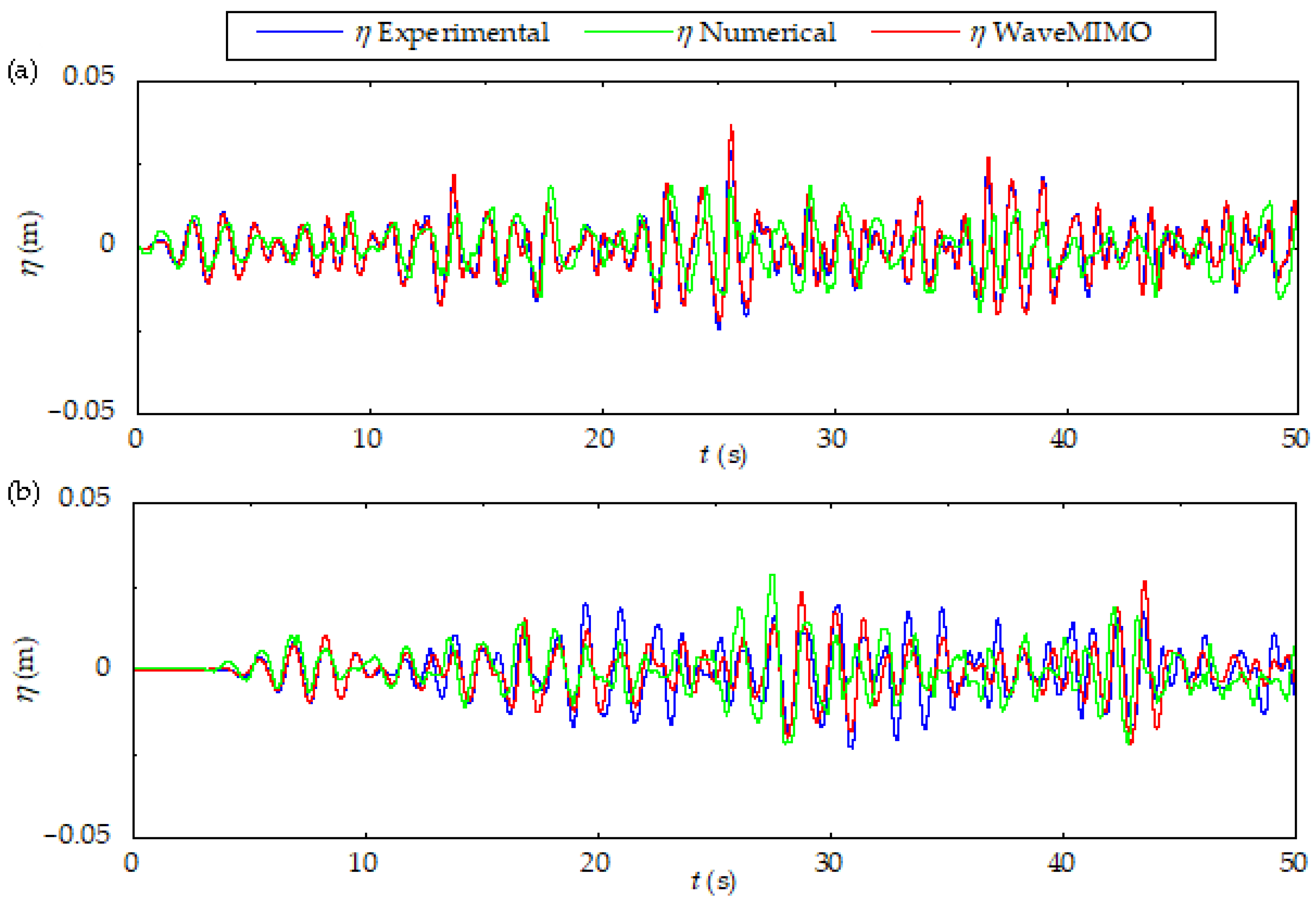Numerical simulations were performed using wave climate data from coastal areas of the Brazilian state of Rio Grande do Sul near the cities of Rio Grande and Tramandaí, with comparative analysis incorporating previous results from the coastal region of city of Mostardas [49]. These assessments enabled the development of theoretical recommendations for implementing the WaveMIMO methodology in the realistic irregular wave generation. Final validation was achieved through qualitative and quantitative comparison with laboratory experimental data from Koutrouveli et al. [34], confirming the methodology’s effectiveness for both wave generation and propagation of these waves.

Among these studies, there are those that focus on the spatial discretization of the computational domain employed, such as the investigation into the discretization of the prescribed velocity BC imposition region. Based on the evaluations and analyses conducted, it was determined that the best results were achieved in Case 1, where it was subdivided into 14 segments. In another study, the mesh sensitivity in the FS region was analyzed. It was possible to establish Case 5 as a theoretical recommendation, where the central segments of the FS region were discretized with greater refinement, totaling 60 computational cells. Additionally, the temporal discretization was investigated, where the time step was related to the mean period. In this evaluation the processing time required was considered to determine the most suitable relation. Thus, the recommendation of using $\mathsf{\Delta }t=T_m/120$, referred to as Case 9, was established. The final study addressed the evaluation of the velocity vector’s location. As a result, Case 11 was determined as the theoretical recommendation, which consists of placing the vector at the upper part of each segment of the prescribed velocity BC imposition region.

In summary, when applying the WaveMIMO methodology for realistic irregular wave generation, the prescribed velocity BC region should comprise 15 segments: the first two, located just below the WLR, with a size of $h/28$, while the remaining 13 segments must have a size of $h/14$. Thus, the FS region on the stretched mesh consists of the first two segments below the WLR and two equally sized segments above it. For spatial discretization, segments near the WLR should contain 20 computational cells, whereas the remaining segments should use 10 cells. The temporal discretization requires a time step of $T_m/120$ and the velocity vector should be considered at the top of each segment in the prescribed velocity BC region.

At last, it is worth highlighting that, when comparing the optimized configuration (Case 12) to recommendations from the previous literature (Case 1) [47], the metrics were reduced by 7.58% (NMAE) and 8.36% (NRMSE) for Rio Grande, while Tramandaí’s sea state showed more modest improvements of 2.36% (NMAE) and 2.44% (NRMSE). Thus, after performing the investigations, it was possible to validate the WaveMIMO methodology against experimental data from Koutrouveli et al. [34]. One can highlight that, in a general way, an excellent agreement between the irregular waves generated with WaveMIMO methodology and the experimental data was achieved, since most employed indicators were below 10%. For future studies, it is suggested to implement a prescribed velocity BC positioned in the upper section of the left wall of the channel. This approach could emulate the effects of wind on the FS of the channel, thereby improving the adjustment of missed crests and troughs, enhancing wave generation accuracy.

References

1. Adesanya, A.; Misra, S.; Maskeliūnas, R.; Damaševičius, R. Prospects of Ocean-Based Renewable Energy for West Africa’s Sustainable Energy Future. Smart Sustain. Built Environ. 2020, 10, 37–50. [Google Scholar] [CrossRef]
2. Hernández-Fontes, J.V.; Felix, A.; Mendoza, E.; Cueto, Y.R.; Silva, R. On the Marine Energy Resources of Mexico. J. Mar. Sci. Eng. 2019, 7, 191. [Google Scholar] [CrossRef]
3. Amarouche, K.; Akpimar, A.; Bachari, N.E.I.; Houma, F. Wave energy resource assessment along the Algerian coast based on 39-year wave hindcast. Renew. Energy 2020, 152, 840–860. [Google Scholar] [CrossRef]
4. Sergent, P.; Baudry, V.; Bonviller, A.D.; Michard, B.; Dugor, J. Numerical Assessment of Onshore Wave Energy in France: Wave Energy, Conversion and Cost. J. Mar. Sci. Eng. 2020, 8, 947. [Google Scholar] [CrossRef]
5. Ribal, A.; Babanin, A.V.; Zieger, S.; Liu, Q. A high-resolution wave energy resource assessment of Indonesia. Renew. Energy 2020, 160, 1349–1363. [Google Scholar] [CrossRef]
6. Patel, R.P.; Nagababu, G.; Kachhwaha, S.S.; Arun Kumar, S.V.V.; Seemanth, M. Combined Wind and Wave Resource Assessment and Energy Extraction along the Indian Coast. Renew. Energy 2022, 195, 931–945. [Google Scholar] [CrossRef]
7. Shadman, M.; Roldan-Carvajal, M.; Pierart, F.G.; Haim, P.A.; Alonso, R.; Silva, C.; Osorio, A.F.; Almonacid, N.; Carreras, G.; Maali Amiri, M.; et al. A Review of Offshore Renewable Energy in South America: Current Status and Future Perspectives. Sustainability 2023, 15, 1740. [Google Scholar] [CrossRef]
8. Liu, J.; Meucci, A.; Liu, Q.; Babanin, A.V.; Ierodiaconou, D.; Xu, X.; Young, I.R. A High-Resolution Wave Energy Assessment of South-East Australia Based on a 40-Year Hindcast. Renew. Energy 2023, 215, 118943. [Google Scholar] [CrossRef]
9. Ye, Z.; Ma, X.; Yang, N.; Cui, L. Assessment of Wave Energy Resources in the Pearl River Estuary of China. Desalin. Water Treat. 2023, 298, 222–232. [Google Scholar] [CrossRef]
10. Pecher, A.; Kofoed, J.P. Handbook of Ocean Wave Energy, 7th ed.; Springer Nature: Berlin/Heidelberg, Germany, 2017. [Google Scholar]
11. Seibt, F.M.; dos Santos, E.D.; Isoldi, L.A.; Rocha, L.A.O. Constructal Design on Full-Scale Numerical Model of a Submerged Horizontal Plate-Type Wave Energy Converter. Mar. Syst. Ocean. Technol. 2023, 18, 1–13. [Google Scholar] [CrossRef]
12. IEA-OES. Annual Report: An Overview of Ocean Energy Activities in 2021; Executive Committee of IEA Ocean Energy Systems: Paris, France, 2022. [Google Scholar]
13. Han, M.M.; Wang, C.M. Coupled analytical-numerical approach for determining hydrodynamic responses of breakwater with multiple OWCs. Mar. Struct. 2021, 80, 103097. [Google Scholar] [CrossRef]
14. Mia, M.R.; Zhao, M.; Wu, H.; Munir, A. Numerical Investigation of Offshore Oscillating Water Column Devices. Renew. Energy 2022, 191, 380–393. [Google Scholar] [CrossRef]
15. Cannata, G.; Simone, M.; Gallerano, F. Numerical Investigation into the Performance of an OWC Device under Regular and Irregular Waves. J. Mar. Sci. Eng. 2023, 11, 735. [Google Scholar] [CrossRef]
16. Maciel, R.P.; Oleinik, P.H.; Dos Santos, E.D.; Rocha, L.A.O.; Machado, B.N.; Gomes, M.d.N.; Isoldi, L.A. Constructal Design Applied to an Oscillating Water Column Wave Energy Converter Device under Realistic Sea State Conditions. J. Mar. Sci. Eng. 2023, 11, 2174. [Google Scholar] [CrossRef]
17. Mocellin, A.P.G.; Maciel, R.P.; Oleinik, P.H.; dos Santos, E.D.; Rocha, L.A.O.; Ziebell, J.S.; Isoldi, L.A.; Machado, B.N. Geometrical Analysis of an Oscillating Water Column Converter Device Considering Realistic Irregular Wave Generation with Bathymetry. J. Exp. Theor. Anal. 2023, 1, 24–43. [Google Scholar] [CrossRef]
18. Chen, W.; Xie, W.; Zhang, Y.; Wang, C.; Wang, L.; Huang, L. Improving Wave Energy Conversion Performance of a Floating BBDB-OWC System by Using Dual Chambers and a Novel Enhancement Plate. Energy Convers. Manag. 2024, 307, 118332. [Google Scholar] [CrossRef]
19. Qian, K.; Chen, L.; Zhou, Y.; Ning, D. Hydrodynamics of an Offshore Multi-Chamber OWC Wave Energy Converter. Energy 2024, 304, 132239. [Google Scholar] [CrossRef]
20. Manimaran, R. Comparative Evaluation of Floating OWC and BBDB Wave Energy Converters by Regular and Irregular Waves Using Numerical Approach. Ships Offshore Struct. 2024, 1–15. [Google Scholar] [CrossRef]
21. Fu, L.; Ning, D.; Wang, R.; Mayon, R. Numerical and Experimental Study on Hydrodynamic Performance of a Land-Based Dual-Chamber OWC Device Under Irregular Waves. Renew. Sustain. Energy Rev. 2025, 207, 114895. [Google Scholar] [CrossRef]
22. Contestabile, P.; Crispino, G.; Russo, S.; Gisonni, C.; Cascetta, F.; Vicinanza, D. Crown Wall Modifications as Response to Wave Overtopping under a Future Sea Level Scenario: An Experimental Parametric Study for an Innovative Composite Seawall. Appl. Sci. 2020, 10, 2227. [Google Scholar] [CrossRef]
23. Musa, M.A.; Roslan, M.F.; Ahmad, M.F.; Muzathik, A.M.; Mustapa, M.A.; Fitriadhy, A.; Mohd, M.H.; Rahman, M.A.A. The Influence of Ramp Shape Parameters on Performance of Overtopping Breakwater for Energy Conversion. J. Mar. Sci. Eng. 2020, 8, 875. [Google Scholar] [CrossRef]
24. Jungrungruengtaworn, S.; Thaweewat, N.; Hyun, B.S. Three-dimensional effects on the performance of multi-level overtopping wave energy converter. IOP Conf. Ser. Mater. Sci. Eng. 2021, 113, 012016. [Google Scholar] [CrossRef]
25. Hubner, R.G.; Fragassa, C.; Paiva, M.S.; Oleinik, P.H.; Gomes, M.N.; Rocha, L.A.O.; Santos, E.D.; Machado, B.N.; Isoldi, L.A. Numerical Analysis of an Overtopping Wave Energy Converter Subjected to the Incidence of Irregular and Regular Waves from Realistic Sea States. J. Mar. Sci. Eng. 2022, 10, 1084. [Google Scholar] [CrossRef]
26. Izzul, M.; Fadhli, M.; Azlan, M.; Noor, M. Parametric study on wave overtopping due to wedge angle and freeboard of wavecat wave energy converter. UMT J. Undergrad. Res. 2022, 4, 37–50. [Google Scholar] [CrossRef]
27. An, S.-H.; Kim, G.-G.; Lee, J.-H. Optimal Design of the Overtopping Wave Energy Converter Based on Fluid–Structure Interaction Simulation. J. Coast. Res. 2024, 116, 578–582. [Google Scholar] [CrossRef]
28. Liu, Z.; Zhang, G. Overtopping Performance of a Multi-Level CROWN Wave Energy Convertor: A Numerical Study. Energy 2024, 294, 130795. [Google Scholar] [CrossRef]
29. Cao, D.; Zeng, H.; He, J.; Liang, H.; Yang, Z.; Ancha, V.R.; Chen, H. A Numerical Investigation of Irregular Wave Overtopping on a 2D Fixed Overtopping Wave Energy Converter. Eng. Appl. Comput. Fluid. Mech. 2025, 19, 2446658. [Google Scholar] [CrossRef]
30. Paiva, M.d.S.; Mocellin, A.P.G.; Oleinik, P.H.; dos Santos, E.D.; Rocha, L.A.O.; Isoldi, L.A.; Machado, B.N. Geometrical Evaluation of an Overtopping Wave Energy Converter Device Subject to Realistic Irregular Waves and Representative Regular Waves of the Sea State That Occurred in Rio Grande—RS. Processes 2025, 13, 335. [Google Scholar] [CrossRef]
31. Fang, Q.; Yang, C.; Guo, A. Hydrodynamic Performance of Submerged Plates During Focused Waves. J. Mar. Sci. Eng. 2019, 7, 389. [Google Scholar] [CrossRef]
32. Wang, C.; Zhang, Y. Hydrodynamic Performance of an Offshore Oscillating Water Column Device Mounted over an Immersed Horizontal Plate: A Numerical Study. Energy 2021, 222, 119964. [Google Scholar] [CrossRef]
33. Thum, G.Ü.; Maciel, R.P.; Oleinik, P.H.; Rocha, L.A.O.; dos Santos, E.D.; Seibt, F.M.; Machado, B.N.; Isoldi, L.A. Numerical Analysis of the Submerged Horizontal Plate Device Subjected to Representative Regular and Realistic Irregular Waves of a Sea State. Fluids 2024, 9, 188. [Google Scholar] [CrossRef]
34. Koutrouveli, T.I.; Di Lauro, E.; das Neves, L.; Calheiros-Cabral, T.; Rosa-Santos, P.; Taveira-Pinto, F. Proof of concept of a breakwater-integrated hybrid wave energy converter using a composite modelling approach. J. Mar. Sci. Eng. 2021, 9, 226. [Google Scholar] [CrossRef]
35. Simonetti, I.; Esposito, A.; Cappietti, L. Experimental Proof-of-Concept of a Hybrid Wave Energy Converter Based on Oscillating Water Column and Overtopping Mechanisms. Energies 2022, 15, 8065. [Google Scholar] [CrossRef]
36. Wan, C.; Yang, C.; Bai, X.; Bi, C.; Chen, H.; Li, M.; Jin, Y.; Zhao, L. Numerical Investigation on the Hydrodynamics of a Hybrid OWC Wave Energy Converter Combining a Floating Buoy. Ocean. Eng. 2023, 281, 114818. [Google Scholar] [CrossRef]
37. Lisboa, R.C.; Teixeira, P.R.; Didier, E. Regular and irregular wave propagation analysis in a flume with numerical beach using a Navier-stokes based model. Defect. Diffus. Forum 2017, 372, 81–90. [Google Scholar] [CrossRef]
38. Zabihi, M.; Mazaheri, S.; Rezaee Mazyak, A. Wave Generation in a Numerical Wave Tank. Int. J. Coast. Offshore Environ. Eng. 2017, 2, 33–43. [Google Scholar] [CrossRef]
39. Windt, C.; Davidson, J.; Ransley, E.J.; Greaves, D.; Jakobsen, M.; Kramer, M.; Ringwood, J.V. Validation of a CFD-Based Numerical Wave Tank Model for the Power Production Assessment of the Wavestar Ocean Wave Energy Converter. Renew. Energy 2020, 146, 2499–2516. [Google Scholar] [CrossRef]
40. Jiang, C.; Yang, Y.; Deng, B. Study on the Nearshore Evolution of Regular Waves under Steady Wind. Water 2020, 12, 686. [Google Scholar] [CrossRef]
41. Oh, S.; Jung, J.H.; Cho, S.K. Higher-Order Spectral Method for Regular and Irregular Wave Simulations. J. Ocean. Eng. Technol. 2020, 34, 406–418. [Google Scholar] [CrossRef]
42. Choi, Y.M.; Bouscasse, B.; Ducrozet, G.; Seng, S.; Ferrant, P.; Kim, E.S.; Kim, Y.J. An Efficient Methodology for the Simulation of Nonlinear Irregular Waves in Computational Fluid Dynamics Solvers Based on the High Order Spectral Method with an Application with OpenFOAM. Int. J. Nav. Archit. Ocean. Eng. 2023, 15, 100510. [Google Scholar] [CrossRef]
43. Kim, Y.J.; Canard, M.; Bouscasse, B.; Ducrozet, G.; Le Touzé, D.; Choi, Y.-M. High-Order Spectral Irregular Wave Generation Procedure in Experimental and Computational Fluid Dynamics Numerical Wave Tanks, with Application in a Physical Wave Tank and in Open-Source Field Operation and Manipulation. J. Mar. Sci. Eng. 2024, 12, 227. [Google Scholar] [CrossRef]
44. Kim, I.-C.; Ducrozet, G.; Bonnefoy, F.; Leroy, V.; Perignon, Y. Real-Time Phase-Resolved Ocean Wave Prediction in Directional Wave Fields: Enhanced Algorithm and Experimental Validation. Ocean. Eng. 2023, 276, 114212. [Google Scholar] [CrossRef]
45. Canard, M.; Ducrozet, G.; Bouscasse, B. Generation of Controlled Irregular Wave Crest Statistics in Experimental and Numerical Wave Tanks. Ocean. Eng. 2024, 310, 118676. [Google Scholar] [CrossRef]
46. Kim, I.-C.; Ducrozet, G. Real-Time Phase-Resolved Ocean Wave Prediction in Directional Wave Fields: Second-Order Lagrangian Wave Models. Ocean. Eng. 2024, 313, 119316. [Google Scholar] [CrossRef]
47. Machado, B.N.; Oleinik, P.H.; Kirinus, E.P.; Dos Santos, E.D.; Rocha, L.A.O.; Gomes, M.; Das, N.; Conde, J.M.P.; Isoldi, L.A. WaveMIMO Methodology: Numerical Wave Generation of a Realistic Sea State. J. Appl. Comput. Mech. 2021, 1, 1–20. [Google Scholar] [CrossRef]
48. Maciel, R.P.; Fragassa, C.; Machado, B.N.; Rocha, L.A.O.; Dos Santos, E.D.; Gomes, M.; Das, N.; Isoldi, L.A. Verification and Validation of a Methodology to Numerically Generate Waves Using Transient Discrete Data as Prescribed Velocity Boundary Condition. J. Mar. Sci. Eng. 2021, 9, 896. [Google Scholar] [CrossRef]
49. Paiva, M.d.S.; Mocellin, A.P.G.; Oleinik, P.H.; Santos, E.D.d.; Rocha, L.A.O.; Isoldi, L.A.; Machado, B.N. Geração de Ondas Irregulares Realísticas Através da Metodologia WaveMIMO: Um Estudo de Caso para Avaliação de Parâmetros. Rev. Thema 2024, 23, 777–802. (In Portuguese) [Google Scholar] [CrossRef]
50. Maciel, R.P.; Machado, B.N.; Oleinik, P.H.; dos Santos, E.D.; Gomes, M. das N.; Isoldi, L.A. Investigation of numerical irregular wave generation using transient discrete data as boundary conditions of prescribed velocity. Defect. Diffus. Forum 2023, 427, 227–235. [Google Scholar] [CrossRef]
51. ANSYS. ANSYS Fluent Theory Guide, Release 20.2; ANSYS Inc.: Canonsburg, PA, USA, 2017. [Google Scholar]
52. Hirt, C.W.; Nichols, B.D. Volume of fluid (VoF) method for the dynamics of free boundaries. J. Comput. Phys. 1981, 39, 201–225. [Google Scholar] [CrossRef]
53. Srinivasan, V.; Salazar, A.J.; Saito, K. Modeling the disintegration of modulated liquid jets using volume-of-fluid (VoF) methodology. Appl. Math. Model. 2011, 35, 3710–3730. [Google Scholar] [CrossRef]
54. Versteeg, H.K.; Malalasekera, W. An Introduction to Computational Fluid Dynamics—The Finite Volume Method; Pearson Education Limited: London, UK, 2007. [Google Scholar]
55. Park, J.C.; Kim, M.H.; Miyata, H.; Chun, H.H. Fully nonlinear numerical wave tank (NWT) simulations and wave run-up prediction around 3-D structures. Ocean. Eng. 2003, 30, 1969–1996. [Google Scholar] [CrossRef]
56. Foyhirun, C.; Kositgittiwong, D.; Ekkawatpanit, C. Wave Energy Potential and Simulation on the Andaman Sea Coast of Thailand. Sustainability 2020, 12, 3657. [Google Scholar] [CrossRef]
57. Gomes, M.N.; Lorenzini, G.; Rocha, L.A.O.; Santos, E.D.; Isoldi, L.A. Constructal Design Applied to the Geometric Evaluation of an Oscillating Water Column Wave Energy Converter Considering Different Real Scale Wave Periods. J. Eng. Thermophys. 2018, 27, 173–190. [Google Scholar] [CrossRef]
58. Oleinik, P.H. O programa Spec2Wave: Manual do usuário; Oleinik, P. H.: Rio Grande, Brazil, 2022. (In Portuguese) [Google Scholar]
59. Benoit, M.; Marcos, F.; Becq, F. TOMAWAC: Software for Sea State Modelling on Unstructured Grids over Oceans and Coastal Seas (Release 6.1); EDF R&D: Paris, France, 2011. [Google Scholar]
60. Holthuijsen, L.H. Waves in Oceanic and Coastal Waters; Cambridge University Press: Cambridge, UK, 2007. [Google Scholar]
61. McCormick, M.E. Ocean Engineering Mechanics: With Applications; Cambridge University Press: New York, NY, USA, 2010. [Google Scholar]
62. Arguilé-Pérez, B.; Ribeiro, A.S.; Costoya, X.; deCastro, M.; Gómez-Gesteira, M. Suitability of wave energy converters in northwestern Spain under the near future winter wave climate. Energy 2023, 278, 127957. [Google Scholar] [CrossRef]
63. Oleinik, P.H.; Maciel, R.P.; dos Santos, E.D.; Rocha, L.A.O.; Machado, B.N.; Isoldi, L.A. Numerical method for the characterization of sea states using realistic irregular waves on computational fluid dynamics simulations for application on wave energy converters. Sustain. Energy Technol. Assess. 2025, 73, 104093. [Google Scholar] [CrossRef]
64. Cardoso, S.D.; Marques, W.C.; Kirinus, E.d.P.; Stringari, C.E. Levantamento batimétrico usando cartas náuticas. In 13ª Mostra da Produção Universitária, Rio Grande; Federal University of Rio Grande: Rio Grande, Brazil, 2014. (In Portuguese) [Google Scholar]
65. Chai, T.; Draxler, R.R. Root mean square error (RMSE) or mean absolute error (MAE)? Arguments against avoiding RMSE in the literature. Geosci. Model. Dev. 2014, 7, 1247–1250. [Google Scholar] [CrossRef]
66. López, I.; Pereiras, B.; Castro, F.; Iglesias, G. Optimisation of Turbine-Induced Damping for an OWC Wave Energy Converter Using a RANS–VOF Numerical Model. Appl. Energy 2014, 127, 105–114. [Google Scholar] [CrossRef]
67. Katsidoniotaki, E.; Shahroozi, Z.; Eskilsson, C.; Palm, J.; Engström, J.; Göteman, M. Validation of a CFD Model for Wave Energy System Dynamics in Extreme Waves. Ocean. Eng. 2023, 268, 113320. [Google Scholar] [CrossRef]
68. Romanowski, A.; Tezdogan, T.; Turan, O. Development of a CFD methodology for the numerical simulation of irregular sea-states. Ocean. Eng. 2019, 192, 106530. [Google Scholar] [CrossRef]
69. Windt, C.; Faedo, N.; García-Violini, D.; Peña-Sanchez, Y.; Davidson, J.; Ferri, F.; Ringwood, J.V. Validation of a CFD-Based Numerical Wave Tank Model of the 1/20th Scale Wavestar Wave Energy Converter. Fluids 2020, 5, 112. [Google Scholar] [CrossRef]
70. Jamieson, P.D.; Porter, J.R.; Wilson, D.R. A Test of the Computer Simulation Model ARCWHEAT1 on Wheat Crops Grown in New Zealand. Field Crops Res. 1991, 27, 337–350. [Google Scholar] [CrossRef]
71. Heinemann, A.B.; van Oort, P.A.J.; Fernandes, D.S.; Maia, A.H.N. Sensitivity of APSIM/ORYZA Model Due to Estimation Errors in Solar Radiation. Bragantia 2012, 71, 572–582. [Google Scholar] [CrossRef]
72. Li, M.-F.; Tang, X.-P.; Wu, W.; Liu, H.-B. General Models for Estimating Daily Global Solar Radiation for Different Solar Radiation Zones in Mainland China. Energy Convers. Manag. 2013, 70, 139–148. [Google Scholar] [CrossRef]
73. Nyang’au, W.O.; Mati, B.M.; Kalamwa, K.; Wanjogu, R.K.; Kiplagat, L.K. Estimating Rice Yield under Changing Weather Conditions in Kenya Using CERES Rice Model. Int. J. Agron. 2014, 2014, 849496. [Google Scholar] [CrossRef]
74. Bounoua, Z.; Chahidi, L.O.; Mechaqrane, A. Estimation of Daily Global Solar Radiation Using Empirical and Machine-Learning Methods: A Case Study of Five Moroccan Locations. Sustain. Mater. Technol. 2021, 28, e00261. [Google Scholar] [CrossRef]
75. El Alaoui, M.; Chahidi, L.O.; Rougui, M.; Lamrani, A.; Mechaqrane, A. Prediction of Energy Consumption of an Administrative Building Using Machine Learning and Statistical Methods. Civ. Eng. J. 2023, 9, 1007–1022. [Google Scholar] [CrossRef]
Figure 1. WaveMIMO methodology flowchart.
Processes 13 01395 g001
Figure 2. Bivariate histogram for the municipality of (a) Rio Grande and (b) Tramandaí.
Processes 13 01395 g002
Figure 3. Illustration of the computational domain used.
Processes 13 01395 g003
Figure 4. Illustration of the stretched mesh regions.
Processes 13 01395 g004
Figure 5. Illustration of the recommended subdivision.
Processes 13 01395 g005
Figure 6. FS discretization: (a) Case 4, (b) Case 5, (c) Case 6.
Processes 13 01395 g006
Figure 7. Illustration of the velocity vector in a segment positioned as follows: (a) upper part, (b) central part, (c) lower part.
Processes 13 01395 g007
Figure 8. Illustration of (a) the physical setup experiment by Koutrouveli et al. [34] and (b) computational domains employed for the validation study.
Processes 13 01395 g008
Figure 9. Qualitative results for the discretization study of the prescribed velocity BC imposition region, evaluated under Rio Grande’s realistic sea state: (a) 0   s t 300   s ; (b) 300   s t 600   s ; (c) 600   s t 900   s .
Processes 13 01395 g009
Figure 10. Qualitative results for the discretization study of the prescribed velocity BC imposition region, evaluated under Tramandaí’s realistic sea state: (a) 0   s t 300   s , (b) 300   s t 600   s , (c) 600   s t 900   s .
Processes 13 01395 g010
Figure 11. Qualitative comparison of the results obtained in the present study with the experimental and numerical data found in [34]: (a) FS elevation at x = 0 m and (b) FS elevation at x = 5.70 m.
Processes 13 01395 g011
Figure 12. Physical phenomenon representation at t = 50 s.
Processes 13 01395 g012