Abstract
Understanding interwell connectivity during water-flooding reservoir development is crucial for analyzing the characteristics of remaining oil and optimizing technical measures. The key lies in establishing an inversion method to identify interwell connectivity. However, traditional history matching methods based on numerical simulation suffer from high computational costs and limited adaptability to complex spatiotemporal dependencies in production data. To address these challenges, this study combines a surrogate model trained using a graph neural network (GNN) and Transformer encoder with a differential evolution particle swarm optimization (DEPSO) algorithm for automated reservoir history matching. The surrogate model is constructed by embedding the capacitance–resistance model (CRM) into a graph structure, where wells are represented as nodes and interwell connectivity parameters as edge features. When applied to the conceptual model, the coefficient of determination (R2) was found to be approximately 0.95 during the training phase by comparing the production data predicted by the surrogate model with the actual observed data. The DEPSO algorithm aimed to minimize the differences between surrogate predictions and observed data, achieving good fitting results. When applied to a complex case study, the average water-cut fitting rate for each production well in its well group reached 87.8%. The results indicate that this method significantly improves fitting accuracy and has substantial practical value.
1. Introduction
During the development and management of oil and gas reservoirs, the establishment of precise numerical models for the reservoirs is advantageous. It allows reservoir engineers to comprehensively understand the characteristics of the reservoirs. Moreover, it facilitates the prediction of reservoir production and the optimization of production performance [1]. Nevertheless, dynamic geological characteristics such as transmissibility and connection volume constitute the principal sources of uncertainty in reservoir numerical models. History matching (HM) [2] is a commonly used method. This approach involves establishing numerical models based on observed history production data and geological information. Subsequently, model parameters are estimated, and the model is calibrated by matching the observed production data.
Since the research on automatic history matching (AHM) [3,4] of oil reservoirs began, numerous promising automatic history matching algorithms have emerged. The application of stochastic methods and intelligent algorithms in dynamic geological modeling has become increasingly widespread. Chakra et al. [5] utilized the genetic algorithm (GA) and adaptive strategies to optimize the physical model parameters of water-flooding oil reservoirs, enhancing both the convergence speed and accuracy of the algorithm. Maschio et al. [6] proposed a method that combines the GA with the simulated annealing (SA), aiming to reduce uncertainties in the data assimilation process by integrating geostatistical implementations. This approach enhances global search capabilities and effectively mitigates uncertainties. With the rising geological complexity of reservoirs and the amount of production data, high computing costs, sensitivity to beginning factors, and difficult-to-solve non-linear problems emerge one after the other. As a result, current research focuses on developing more efficient and robust automatic history fitting technologies.
The traditional AHM of oil reservoirs is typically achieved through model-based history matching methods. Sun et al. [7] introduced the Capillary number (Ca) and the BG equation to develop a novel numerical reservoir simulator. This simulator is capable of accurately capturing the dynamic characteristics of residual oil saturation as it varies with water flooding velocity. In the application to the S oilfield in Bohai Bay, the history matching performed using this new simulator significantly improved matching accuracy compared to Eclipse, thereby robustly validating its superior performance. Kazemi et al. [8] employed production data and four-dimensional seismic data, utilizing parameter updating schemes such as global univariate, regional multivariate, and local multivariate approaches. These schemes effectively improved the history matching results for the water-flooding reservoir in the case study. Li et al. [9] systematically demonstrated best practices for assisted history matching by adopting the Design of Experiment (DoE) methodology. This approach embodies optimal practices in water injection development, enhancing the accuracy of reservoir performance predictions and management efficiency through meticulous data analysis and model construction. Forouzanfar et al. [10] conducted a study on multi-solution search-assisted history matching in water injection development using the constrained iterative ensemble smoother method. Avansi et al. [11] employed a synchronous history matching method that integrates reservoir characterization with reservoir simulation studies in water injection development. By concurrently calibrating multiple objective functions while maintaining the consistency of the geological model, they enhanced the accuracy and reliability of the history matching process. Xu et al. [12] utilized a history matching method that involves the integrated analysis of multi-source data, the application of advanced numerical algorithms, and comprehensive consideration of model uncertainties. This approach enhances the accuracy and reliability of reservoir simulation in water injection development processes. However, these numerical methods often require extensive numerical simulations, with each simulation run potentially taking minutes to hours [13,14,15]. To alleviate the computational burden of numerical simulations during the optimization process and enhance the operational efficiency of AHM, surrogate models are integrated into the AHM methods [16,17,18,19].
Based on surrogate models, AHM methods can be categorized into online and offline approaches. Online methods involve continuous dynamic sampling during the solution process to construct and optimize the surrogate model. The core characteristic of this approach is that the surrogate model is not static during the history matching process, but rather, it is continuously updated and adjusted based on new data and information to more accurately reflect the actual state of the reservoir. The adaptive importance sampling algorithm proposed by Li et al. [20] is a typical example of an online AHM method, which efficiently solves the multi-modal Bayesian inversion problem by dynamically updating the proposal distribution and using online clustering techniques. Zhang et al. [21] proposed an adaptive multi-fidelity Markov chain Monte Carlo (AM-MCMC) algorithm, which centers around establishing an adaptive Gaussian Process (GP) online surrogate model. By dynamically updating the GP surrogate model and intelligently allocating multi-fidelity resources, this method enables efficient Bayesian inference for hydrological system inversion. Ma et al. [22] employed a dynamically updated Radial Basis Function (RBF) online surrogate model to reduce simulation calls, with algorithm parameters automatically adjusted during the optimization process. By balancing exploration and exploitation using an intelligent sampling strategy, this method achieves multi-solution preservation and efficient uncertainty quantification, providing a new solution for complex reservoir history matching problems. Qiao et al. [23] presented a novel surrogate model sequential sampling method for dynamic system design and optimization, which significantly incorporates the core idea of online adaptive history matching techniques. By dynamically updating the surrogate model and utilizing intelligent sampling strategies, this method efficiently simulates and optimizes complex dynamic systems. Janatian [24] proposed an optimization control framework that integrates online adaptive history matching technology, enabling efficient and precise regulation of reservoir production through dynamic surrogate model updates and real-time data feedback. Online methods can reflect the latest model state in real time but come with relatively high computational costs. Offline methods, on the other hand, involve pre-constructing a trained surrogate model using the entire known training dataset and using this pre-trained surrogate model for rapid predictions, significantly enhancing computational efficiency. The core objectives of offline methods are to replace high-cost simulations, accelerate optimization processes, and handle high-dimensional, non-linear data. The construction process includes experimental design, data generation, model selection and training, model validation, and model application. In recent years, offline methods have witnessed rapid development, with deep learning-based surrogate models achieving remarkable success in solving history matching problems involving high-dimensional spatial distribution parameters. Many researchers have used Artificial Neural Networks (ANNs) to establish non-linear relationships between geological conditions and dynamic production. Canchumuni et al. [25] combined an offline-trained Deep Generative Model (DGM) with ensemble smoothers (ESs) to construct an efficient offline AHM framework that addresses the high-dimensional non-Gaussian challenges in geological facies history matching, providing new insights into surrogate modeling for complex systems. Qin et al. [26] employed an offline surrogate model based on a Recurrent Neural Network (RNN) combined with optimization algorithms to achieve efficient optimization of geothermal reservoir energy extraction. Liu et al. [27] proposed a hybrid offline surrogate model based on Ensemble Empirical Mode Decomposition (EEMD) and a Long Short-Term Memory network (LSTM) for oilfield production prediction. Aghayev et al. [28] introduced an offline surrogate-assisted optimization framework based on classification-constrained modeling for oilfield recovery optimization under high constraints. In previous studies, there has been a lack of sufficient consideration for the complex dependencies between data and well connectivity. During water-flooding development, phenomena such as wellbore scaling and corrosion may occur, affecting the accuracy of interwell connectivity analysis. Studies have shown that the addition of chemical inhibitors can effectively control these issues [29], thus ensuring the reliability of production data. Given that numerous scholars have conducted in-depth research on this topic, it will not be considered in the subsequent analysis of this paper. Therefore, while online and offline approaches have made significant progress in the construction and application of agent models, traditional machine learning and deep learning models still face challenges in the face of more complex, dynamic data scenarios with rich relational structures. Especially in the petroleum industry, production data not only have high dimensionality and non-linearity, but they also often contain complex spatial relationships and temporal dependencies, which requires the agent model to capture and utilize these complex relationships more effectively. In recent years, the rise of graph neural networks has provided a new perspective for solving these problems.
Graphs, a type of data structure, have been widely employed in many industries because they can effectively portray complex relationships between items. GNN constructs a complex and deep neural network model by combining node feature information and graph structural data [30,31]. Wang et al. [32] proposed an interpretable recurrent GNN. This network aims to construct an interactive process that simulates flow between wells. It describes the hidden states of wells and the exchange of energy information among them, continually updating these states both spatially and temporally. Lu et al. [33] employed a GNN model. They trained a lithology identification model based on constructed graphs. The model connects samples with adjacent depths and similar logging response features to logging features with similar operational intents. This addresses the challenge of lithology identification in continental shale oil reservoirs using well logging data. Huang et al. [34] developed a novel surrogate model based on deep learning. This model integrates GNN with LSTM techniques. It is applied to predict dynamic oil and water volumes under various well control conditions. Compared with the traditional agent modeling methods, the method based on a graph neural network can represent more complex mapping relationships and has higher performance and model interpretability. The prediction of the reservoir water cut is a problem of time series prediction based on production history. However, GNN focuses on spatial features in mining data, without considering the impact of historical data on reservoir production.
Vaswani et al. [35] proposed a Transformer model in 2017. Its core idea is to introduce an attention mechanism, which is mainly applied to natural language processing. With further research, scholars gradually found its advantages in sequence data processing, which can be applied to a variety of sequence learning tasks, including time series prediction. In combination with the GNN model, Transformer calculates the relative importance of different nodes through a self-attention mechanism, assigning a weight to each neighbor node. This operation allows the model to focus on the more critical nodes and capture the long-distance dependencies in the series, thereby improving the accuracy and generalization of time series predictions. It is worth noting that, in the field of gas flooding optimization, existing research has begun to explore methods that combine Transformers with particle swarm optimization (PSO) algorithms. For example, Gao et al. [36] proposed an intelligent optimization technique for gas flooding based on a multi-objective optimization method, which achieves efficient and accurate optimization of the gas flooding process by combining surrogate models, PSO algorithms, and Transformer models. Although the specific application scenario of this research differs from that of the present study, its research approach and technical route provide valuable references for this paper.
The prediction of the reservoir water cut (WWCT) is related to both spatial and temporal characteristics. Therefore, in this study, a combined prediction model of GNN-Transformer (GNT) is constructed as a surrogate model. The CRM model proposed by Yousef et al. [37] uses two key parameters to evaluate the interwell connectivity and fluid storage capacity of each injection–production well pair. And the CRM model can effectively describe the production capacity of a field. Based on the CRM model, with the well point as a node, well connectivity as an edge feature, and the well pattern structure as the graph structure, a graph neural network model is established. Then, the advantages of Transformer, such as the self-attention mechanism, parallel processing capability, and time series processing capability, are organically integrated with Transformer to build a reservoir water cut prediction model. The optimization algorithm is selected as the differential evolution particle swarm fusion algorithm. The algorithm combines the PSO with the differential evolution algorithm (DE) to enhance the population diversity, improve the individual’s ability to jump out of the local optimal solution, and accelerate the convergence rate. The offline AHM combined with the DEPSO method is used to optimize the objective function, composed of the prediction results of the agent model and the real value, and to find the best solution in line with the model.
In this study, we provide a detailed introduction to the construction of the GNT surrogate model, the DEPSO optimization algorithm, and the DEPSO history matching framework based on the surrogate model in Section 2. In Section 3, we train and evaluate the proposed surrogate model and history matching efforts using both a conceptual reservoir case and a complex reservoir case. The conclusions are presented in Section 4.
2. Methods
2.1. GNN Surrogate Model
The principles of a GNN. In a graph, each node identifies its neighboring nodes through an adjacency matrix and updates its own node features via an information aggregation mechanism. The objective of a GNN is to learn a state embedding vector for each node through a series of information passes [38,39]. This process enables the model to capture complex relationships and features within graph data.
Here, represents the state embedding vector; is the local transition function; is the local output function; denotes the feature vector of node ; represents the feature vector of the edge associated with node ; denotes the state vector of the neighboring nodes of node ; represents the feature vector of the neighboring nodes of node ; is the output vector.
For all nodes in the graph with respect to and , we stack all feature vectors, state vectors, node features, and output vectors, denoting them as , , , and , respectively. This results in a global transition function and a global output function. Consequently, Equations (1) and (2) can be further expressed as follows:
GNNs use traditional iterative methods to compute the state vectors, which can be expressed as follows:
Here, represents the current layer number of message passing or the number of iteration cycles of message passing. denotes the tensor of the -th iteration cycle. For any initial value of , the solution to Equation (3) can be obtained through the rapid convergence of Equation (5). If target information is utilized for supervised learning, the loss function can be expressed as follows:
Here, represents the total number of supervised nodes, while and denote the true values and predicted values of the nodes, respectively. The learning process of the loss function relies on the gradient descent strategy, and the process includes the following steps:
- The state is iteratively updated for rounds according to Equation (1) until it approaches the fixed-point solution of Equation (3) at time . At this point, the obtained will be close to the fixed-point solution ≈ .
- The gradient of the weights is calculated from the function.
- The weights are updated using the gradient calculated in step 2.
Transformer. The production performance of a water-flooding reservoir is closely related to many geological and engineering factors such as the formation pressure and water injection rate. And it shows strong correlation and causality in time, constituting time series data. The limitations of a GNN in processing time series data have led to the introduction of Transformer. By leveraging Transformer’s self-attention mechanism and focusing on key nodes that significantly impact production dynamics, it effectively analyzes and handles the aforementioned complex time series problems. Transformer is a network architecture based on the attention mechanism. This architecture mainly consists of an encoder and a decoder. The typical structure of Transformer is shown in Figure 1.
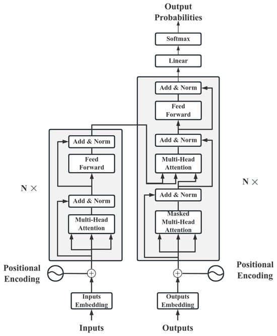
Figure 1.
Diagram of the Transformer model structure.
The encoder component consists of an input layer, a positional encoding layer, and a stack of four identical encoder layers. Each layer primarily comprises two sub-layers, a self-attention layer, and a feedforward neural network layer. After each sub-layer, residual connections and layer normalization operations are used. These operations help the encoder capture the dependencies of all positions in the input sequence, effectively preventing the gradient disappearance problem.
The decoder has a similar architecture to the encoder and is responsible for converting the encoder’s information into a target sequence. The decoder consists of several identical layers, each with three sub-layers, the self-attention layer, the encoder–decoder attention layer, and the feedforward neural network layer. After each sub-layer, there are residual joins and layer normalization operations. These operations ensure that the decoder generates the sequence correctly. They help the decoder take into account the previous output and avoid being influenced by future information.
The multi-head self-attention mechanism in Transformer is one of the core components of the Transformer model. It enhances the ability of the model to understand and generalize complex sequence tasks. The input sequence is first linearly transformed into multiple query, key, and value matrices. These matrices are then divided into smaller parts, each corresponding to an attention head. In each attention head, the attention score is obtained by calculating the dot product of the query with the key. After these scores are normalized by Softmax, the values are weighted and summed as weights to obtain an output representation of the attention head. Finally, all the output representations are concatenated, and the final output is obtained through a linear transformation. This approach allows the model to capture dependencies and nuances in the sequence from multiple perspectives, significantly improving the model’s ability to handle complex sequence tasks. The bull attention is calculated as follows:
Here, denotes the parameter matrix for the output projection; represents the self-attention distribution for the -th head; , , and denote the projection matrices for the query, key, and value of the -th head, respectively. The computation of for each head is conducted as follows:
Here, represents the dimension of the key.
2.2. Development of the Surrogate Model
Graph structure establishment. The CRM is conceptualized as a graph structure, where oil wells and water wells are regarded as nodes in the graph. The connectivity between wells is mapped as edges between nodes, and the well-to-well connectivity is parameterized as edge features. Based on this, a connection network from injection wells to production wells is constructed. Considering that the production dynamics of injection–production wells are different at different production time points, the characteristic parameters of the GNN model need to be dynamically adjusted accordingly. Therefore, a specific graph structure is constructed for each extraction time point. Therefore, a specific graph structure is constructed for each mining time point. For a particular extraction, the input features of the injection well node cover the water injection volume at the current extraction time, the total water injection volume, the well location data, the address feature where it is located, and the water content at the last extraction time. Correspondingly, the input features of the production well node cover the fluid production volume at the current extraction time, the total fluid production volume, the well location data, the address characteristics where it is located, and the water content rate at the last extraction time.
Model establishment. Build a GNT surrogate model to predict the WWCT of each production well. The model architecture is shown in Figure 2. It is mainly divided into the following modules: the Graph Convolutional Network (GCN) layer, the Position Encoding Module, the Transformer Encoder Module, and the final Prediction Module. In the GCN layer, spatial features are extracted from the graph structure of reservoir data. The input data include the node feature matrix, adjacency matrix, and edge features. The node feature matrix describes the attribute information of each well (such as well type, permeability, porosity, injection volume, and production volume), the adjacency matrix describes the connection relationships between wells, and the edge features describe the connectivity parameters between wells (such as transmissibility and connection volume). The GCN convolution operation is achieved by aggregating the node features of the graph structure with the features of their neighboring nodes. The feature update process for each node depends on the feature information of its neighboring nodes. Since the edge features between well nodes also influence the production dynamic indicators, this paper adopts an edge feature-enhanced message-passing mechanism in the GCN layer, introducing edge features into the information propagation process. When aggregating neighboring node features, the edge features are weighted to adjust the strength of information propagation between nodes:
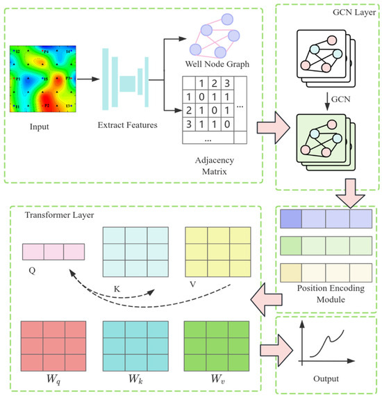
Figure 2.
Architecture diagram of the GNT surrogate model.
Here, represents the feature representation of node at layer , is the non-linear activation function, is the normalization coefficient, and denotes the weight matrix for edge features, which is a learnable parameter used to perform linear transformations on edge features, so as to take edge information into account when aggregating node features. It enables the model to adjust the information transmission between nodes according to edge features, thereby more accurately capturing the relationships in the graph. represents the edge features, is the element-wise multiplication, and is the weight matrix for node features, used to perform linear transformations on node features to update the representation of nodes during the aggregation operation. It allows nodes to learn more complex feature representations, thus better capturing the structural information in the graph. This aggregation mechanism allows the model to dynamically adjust the strength of message propagation based on edge features, thereby more flexibly capturing the relationships between nodes.
In the specific implementation, the model employs a three-layer GCN to extract spatial features. The first GCN convolutional layer receives 7-dimensional node features as input and aggregates first-order neighbor information of nodes through the adjacency matrix and edge features, capturing local structural characteristics. Through linear transformation and non-linear activation functions, the node features are mapped to a 64-dimensional hidden space. The second GCN convolutional layer, building upon the previous layer, further aggregates second-order neighbor information of nodes, capturing broader local structural features. The third GCN convolutional layer aggregates third-order neighbor information of nodes, capturing global structural features, and compresses the features to 32 dimensions. Through the final convolutional operation, the model generates node feature representations that incorporate global information, providing high-quality feature inputs for downstream tasks. By stacking multiple layers, nodes can progressively integrate information from multi-order neighbors, thereby generating rich feature representations.
Before the output data from the GCN are fed into the Transformer, positional encoding is applied. The purpose of this step is to add positional information to each element in the sequence, enabling the Transformer to distinguish elements at different positions. In this study, positional encoding is generated using a combination of sine and cosine functions. First, a positional encoding matrix is initialized with a certain size, including the maximum length of the sequence and the dimensionality of the encoding vector, which matches the output dimension of the GCN. According to Equations (11) and (12), sine and cosine values are computed for each position and each dimension, respectively. The generated positional encoding matrix is then stored as a parameter of the model.
Here, represents the position index of the input sequence, represents the positional encoding with a dimensionality of , and is the dimensionality of the positional encoding vector. In this study, the sample dataset used has defined timestamps (e.g., the mining status is recorded every 30 days). Therefore, the graphs corresponding to each mining operation are numbered sequentially in chronological order, with (where represents the total number of time steps). The output of the GCN is a node feature matrix , where is the number of nodes, and is the output dimension of the GCN. To transform the GCN output into a sequence format suitable for Transformer input, it is first reshaped into a three-dimensional tensor, adjusting the shape of from to , where represents the batch size. The positional encoding matrix is then added to the GCN output , embedding positional information into each node feature. Through broadcasting, the positional encoding matrix is automatically expanded to match the shape of the GCN output. This approach enables the positional encoding to convert the GCN output data into a sequence format with positional information, thereby meeting the input requirements of the Transformer.
In the Transformer layer, since the reservoir water cut prediction task is a typical time series prediction problem, which aims to predict the water cut value at a future time point based on historical data, time series prediction tasks do not require generating sequential data but rather directly perform feature extraction and regression prediction on the input sequence. Therefore, this module is implemented using only the encoder. The encoder layer consists of a multi-head self-attention mechanism and a feedforward neural network, and it employs layer normalization and residual connections to accelerate model convergence and enhance training stability. Specifically, the data after positional encoding serves as the input to the Transformer layer. The number of attention heads is set to 4, the number of encoder layers is 2, and the hidden layer dimension of the feedforward neural network is 128. Self-supervision and the masking mechanism are crucial for the model to effectively capture long-range dependencies in the sequence. The core idea of self-supervision is to prevent the model from “peeking” at future information during training through masking techniques, thereby ensuring that the model can only rely on current and past information for prediction. Considering the dynamic nature of reservoir changes, for example, when predicting the water cut of a well, the model can only rely on historical data from that well and its neighboring wells, rather than future data. In this paper, an upper triangular mask matrix is generated based on the sequence length (i.e., the number of nodes), defined as follows:
Here, and , respectively, represent the position indices in the sequence. When , , indicating that the information at position can be used to predict position ; otherwise, , indicating that the information at position is masked and cannot be used to predict position . During the forward propagation process of the Transformer encoder, the input data consist of the positionally encoded data and the mask matrix, which are passed to the self-attention mechanism. In the self-attention mechanism, the mask matrix is added to the attention score matrix to restrict the attention weights for each position. Ultimately, the feature representations processed by multiple encoder layers are obtained. The output of the Transformer is adjusted along the sequence length dimension and mapped to the final output dimension through a fully connected layer, thereby achieving the prediction of the water cut for each production well.
Surrogate model training. In model training, the Mean Squared Error (MSE) is used as the loss function. It compares the predicted values with the true values. The MSE calculates the average of the square of the difference between the actual and predicted values.
Here, is the total number of data; is the true value of the -th sample; is the predicted value of the -th sample.
During training, the Adam algorithm is employed to optimize the loss function, utilizing the backpropagation method to adjust and update the model’s parameters. The learning rate is a crucial hyperparameter that significantly impacts the performance of the Adam algorithm. The initial learning rate is set to 0.001. As training progresses, if the error is observed to stagnate or the convergence rate slows down, the learning rate can be reduced to further refine the model’s training, for instance, by multiplying the learning rate by 0.9.
Evaluation model. The correlation coefficient R2 is used to evaluate the performance of the model. R2 is an indicator used to evaluate the goodness of fit of the regression model. The value range of R2 is [0, 1]. The closer the value of R2 is to 1, the closer the predicted value of the model is to the true value and the better the performance.
Here, is the average value of the simulated real data.
2.3. History Matching Workflow Based on the Hybrid Algorithm of DEPSO
Objective function. In AHM methods, it is necessary to define an objective function to reasonably quantify the error between predicted results and actual values. Based on Bayesian theory, the objective function for reservoir simulation history matching problems is determined, as shown in Equation (16), to find a set of interwell connectivity parameters that conform to the actual reservoir conditions and minimize the objective function.
Here, is the objective function for history matching, is a vector composed of interwell connectivity parameters, represents the true values, denotes the predicted values from the surrogate model, and is the dynamic covariance matrix.
For actual reservoirs, after conducting reservoir geological studies, we have a certain understanding of some reservoir characteristics, such as average permeability, porosity, connection volume, and transmissibility. Therefore, the interwell connectivity parameters need to satisfy certain conditions:
Here, and are vectors composed of the lower and upper bounds of the connectivity parameters, respectively. Generally, the lower bound is 0, while the specific lower and upper bounds need to be considered based on the physical parameters of the reservoir. represents the total connection volume of the reservoir. Since reservoir reserves are relatively reliable, the sum of the connection volume of each connected unit should remain basically unchanged or have very small changes.
Particle swarm optimization algorithm. The PSO algorithm is a novel swarm-based intelligent optimization method inspired by the predator behavior of bird flocks and fish schools [40]. The fundamental idea is as follows: First, a population consisting of multiple individuals is randomly initialized, where each individual represents a potential candidate solution to the problem at hand. Next, an evaluation function is used to assess the quality of these solutions. Then, individuals dynamically update their flight velocities and positions not only based on their flight behaviors but also by referring to the flight experiences of the entire population. Ultimately, the individuals in the population gradually approach the optimal position in the solution space until the optimal solution converges and stabilizes. The updated formulas for particle velocity and position are given as follows:
Here, represents the velocity of the particle; is the inertia parameter; and are the individual acceleration constant and the swarm acceleration constant, respectively; is a random number between (0, 1); is the best value searched by the -th particle; is the best value searched by the entire swarm; is the current position of the -th particle.
The PSO algorithm is renowned for its simple implementation, convenient parameter setting, and efficient operation. However, as the dimensionality of the search space increases, the solution space that the algorithm needs to explore also expands dramatically. The particle swarm algorithm primarily relies on the guidance of inertia weight, personal best, and global best when updating particle velocities and positions. But this update method may lack sufficient dynamic adjustment capability, making it difficult for particles to flexibly adjust their strategies during the search process. When particles approach local optimal solutions, due to the absence of an effective escape mechanism, they can easily fall into local optimal regions and fail to continue exploring to find the global optimal solution.
Differential evolution algorithm. The DE algorithm is a highly efficient global optimization algorithm rooted in swarm intelligence theory. It directs the optimization search through cooperation and competition among individuals within the swarm. Essentially, DE is a self-organizing minimization method. Its fundamental principle involves perturbing an existing vector using different vectors randomly selected from the population, ensuring that every vector is disturbed. This increases population diversity, enabling the algorithm to escape local optimal solutions. The core mechanisms of DE encompass three primary operations: mutation, crossover, and selection. These operations collectively act on the population, driving its evolution. Starting from a randomly generated initial population, the algorithm evaluates individuals by calculating their fitness values and then decides whether to continue the evolution based on termination criteria. In each generation, the algorithm constructs descendant individuals by crossing and merging a third individual with a weighted difference vector derived from two different individuals randomly selected from the population. Subsequently, the fittest individuals are selected based on their fitness values to form a new population, and individuals are updated accordingly, generating a more competitive population. This process not only enhances the diversity of the population but also enables the algorithm to continuously approach the optimal solution in the search space, demonstrating strong global search capability and optimization performance.
In the DE algorithm, individual mutation is achieved through a differential strategy:
Here, , , and are randomly selected vectors, each distinct from the others; represents the mutation operator, where a larger makes it less likely to fall into local extreme points, while a smaller is more conducive to converging to local extreme points.
In continuous iterations, newly generated mutated individuals are allowed to cross and recombine with individuals from the original population at a certain probability, enhancing population diversity. Crossover operations are performed on the mutated individuals based on the following formula to obtain temporary individuals = (, ⋯, ):
Here, = 1, 2, ⋯, N, = 1, 2, ⋯, M, is a random number, is a random number between [0, 1], and is the crossover probability.
Finally, for each individual in the current generation, a judgment is made between its and , and the one with the best fitness is selected as the individual at the same position in the next generation. The competitive selection strategy is as follows:
If the individual obtained through crossover is not worse than the original individual, it replaces the original as a new-generation individual. Otherwise, the new generation of individuals remains the same as the original.
Differential evolution particle swarm algorithm. In the early stages of optimization using the PSO algorithm, the convergence speed is relatively fast. However, in the later stages of the solution process, if no new particles are available to update the currently found best position, the other particles in the swarm will tend to converge toward this known best position [41]. When all particles cluster within a small area, the change in fitness values will become slow or even cease altogether, leading to the phenomenon of premature stagnation in the algorithm. The DE algorithm, on the other hand, possesses strong search capabilities for finding the global optimal solution and is highly robust [42]. However, achieving high-precision solutions requires a significant amount of time.
The DEPSO algorithm first evolves the individual vectors through the mutation operation of DE. Subsequently, it calculates the fitness value of each individual in the population and stores both the individual best positions and the global best position. Then, it updates the velocity and position vectors of all individuals using the PSO algorithm (Algorithm 1). This algorithm skillfully combines the tracking, memory, and flexible search strategy adjustment capabilities of the DE algorithm with the operational efficiency of the PSO algorithm. This combination prevents certain individuals in the algorithm from falling into local optimal solutions due to acquiring erroneous information, thereby enhancing the algorithm’s global search capabilities [43]. It effectively avoids premature convergence of the algorithm and further strengthens its ability to solve complex optimization problems.
| Algorithm 1. The optimization process of the DEPSO algorithm |
| 1: Randomly generate initial position matrix , randomly generate initial velocity matrix 2: Initialize individual optimal values , calculate fitness values, initialize global optimal values 3: for = 1 to : 4: for = 1 to : 5: Randomly select three different individuals x_r1, x_r2, x_r3 (where r1, r2, r3 ≠ i) from the current population 6: v_n = x_r1 + × (x_r2–x_r3) 7: Generate a trial vector u_n whose elements are obtained by crossing the elements of v_n and x_n with a probability CR. 8: Evaluate the fitness of u_n and , update if the fitness of u_n is better 9: calculate speed variable 10: calculate position variable 11: Evaluate the fitness of and, update if the fitness of is better 12: Evaluate the fitness of and , update if the fitness of is better 13: End for 14: End for |
2.4. History Matching Framework
As shown in Figure 3, the history matching framework based on the GNN surrogate model involves the following four parts. First, the basic geological reservoir model is constructed, and the corresponding dataset is obtained by means of CRM. Secondly, the generated data are used to train the GNT surrogate model. Then, the trained surrogate model is combined with the DEPSO algorithm to optimize the interwell connectivity parameters. Finally, the final history matching model is obtained.
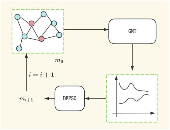
Figure 3.
History matching framework based on GNT surrogate model and DEPSO.
3. Case Study
In this section, two two-dimensional heterogeneous reservoir models are studied, each using a CRM approach to generate training and test datasets. Each case dataset is used to train and evaluate the GNT surrogate model, and then the surrogate model and optimization algorithm are used to solve the historical fitting problem.
To ensure the reproducibility of the experiments and the accuracy of the results in this study, the hardware and software configurations used during the experimental process are described. The experiments in this study are conducted based on the Python 3.11.11 programming language and the PyTorch 2.6.0 deep learning framework. For the GCN component, the code defines a custom class that inherits from MessagePassing, implementing a custom graph convolutional layer for integrating node and edge features. Additionally, the PyTorch built-in module torch.nn is utilized for the Transformer component. The specific configuration parameters of the experimental environment are listed in Table 1.

Table 1.
Experimental environment configuration.
3.1. CASE1: Conceptual Reservoir Case
The two-dimensional heterogeneous conceptual reservoir model is established, and Figure 4 illustrates the well locations and their connectivity within this model. The reservoir parameters are set as follows: The reservoir contains 5 injection wells and 4 production wells. The reservoir thickness is 8.5 m, the porosity is 0.3, and the average permeability is 950 mD. The initial reservoir pressure is 8 MPa, with viscosities of 43 mPa⋅s and 1.1 mPa⋅s for crude oil and water, respectively. The compressibility of crude oil is 2.365 × 10⁻⁵ MPa−1, the compressibility of formation water is 6.358 × 10⁻⁵ MPa−1, and the compressibility of rock is 17 × 10−5 MPa−1.
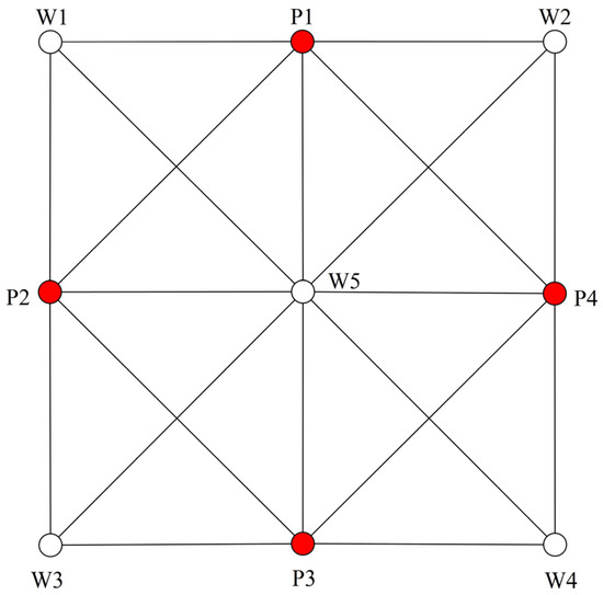
Figure 4.
The point locations and connectivity relationships in the conceptual reservoir case study. Among them, red circles represent production wells, and white circles represent injection wells.
Surrogate model training and evaluation. Using preset reservoir parameters, 2000 sample datasets were generated by means of CRM. Of these, 1500 samples were used as training data, and 500 samples were used as test data. Each group of samples covers 100 mining cycles, with a time step of 30 days per cycle, and includes multi-dimensional time series features (such as water injection volume, liquid production volume, etc.). Based on the different mining cycles, each sample is processed into 100 graph data points. During model training, the batch size is set to 100 and the total number of training cycles to 100.
The GNN surrogate model and the GNT surrogate model were trained separately, and the training loss values of both models were recorded. The results are shown in Figure 5. It was observed that, as the number of training epochs increased, the loss values of both models gradually decreased and tended to stabilize. The training loss value of the GNT model was lower compared to that of the GNN model. In terms of model evaluation, the R2 score of the GNN model approached 0.6, while the R2 score of the GNT model exceeded 0.95, demonstrating higher prediction accuracy. The accuracy of the surrogate models was validated using test data, as shown in Figure 6. The GNT surrogate model outperformed the GNN surrogate model, providing accurate predictions and being capable of replacing the numerical simulation process in AHM.
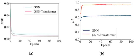
Figure 5.
Loss and correlation coefficient of the training set. (a) Description of the MSE of the two surrogate models during the training process. (b) Description of the R2 of the two surrogate models during the training process.
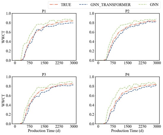
Figure 6.
WWCT comparison.
History matching results. In this study, a sample was randomly selected from the test dataset, and the differential evolution particle swarm optimization algorithm combined with the surrogate model was used to determine the optimal interwell connectivity parameter values. In this process, the population size is set to 50, and the algorithm is set to terminate when it iterates 100 times. Table 2 and Table 3 list the comparison data between the connectivity parameters obtained by DEPSO inversion and the actual connectivity parameters. Figure 7 and Figure 8, respectively, show the comparison of transmissibility and connection volume before and after fitting. In order to further verify the fitting effect, the fitting connectivity parameters and corresponding production dynamic data were fed into the simulation software to obtain the water cut of each production well. Figure 9 presents a comparison of the WWCT curves fitted to the connectivity parameters over the past 900 days, revealing that both exhibit analogous trends. Based on the above comparative data analysis, the combination of the GNT surrogate model and the DEPSO algorithm is an effective and reliable reservoir inversion method.
Table 2.
The actual transmissibility versus the transmissibility obtained through history matching using the DEPSO algorithm.
Table 3.
The actual connection volume versus connection volume obtained through history matching using the DEPSO algorithm.
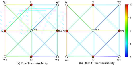
Figure 7.
Transmissibility comparison.
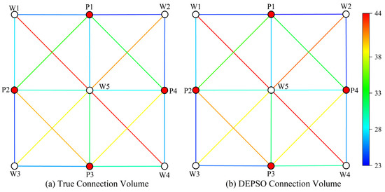
Figure 8.
Connection volume comparison.
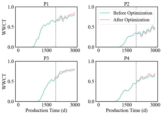
Figure 9.
Comparison of real WWCT and fitted WWCT.
3.2. CASE2: Complex Reservoir Case
An example of a complex reservoir is selected to test the proposed method. Figure 10 shows the initial reservoir model with 8 injection wells and 13 production wells. The reservoir model takes a 30-day time step, with a total production time of 4500 days. A CRM model is built based on reservoir geological data, which include 2000 sample datasets for training models and historical fitting.
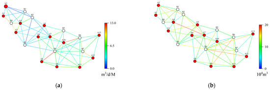
Figure 10.
Initial reservoir model. (a) Description of the transmissibility of the model. (b) Description of the connection volume of the model.
Similar to the conceptual model, 1500 samples were used as training data, and 500 samples were used for testing and validation. Each data file was processed into 150 graph data points based on a production period of 4500 days and a time step of 30. The model input parameters included node features, edge features, and a relationship matrix, while the output was the WWCT for each production well. The surrogate model based on a GNN and the surrogate model based on GNT were trained separately. The loss values and correlation coefficient scores for each epoch were recorded for comparison, as shown in Figure 11. Regarding the MSE, at the early stages of iteration, the MSE of the GNN model decreased rapidly and then stabilized. In contrast, the MSE of the GNT model decreased at a relatively slower rate. However, as the number of iterations increased, the MSE of the GNT model gradually decreased and stabilized in the later stages, demonstrating overall superior performance compared to the GNN model. For the correlation coefficient scores, at the beginning of the iteration, the R2 values of both the GNT model and the GNN model increased rapidly. The R2 value of the GNN model stabilized after approximately 20 iterations, approaching 0.6. As the number of iterations increased, the R2 value of the GNT model continued to rise throughout the entire iteration process, with its correlation coefficient score, R2, approaching 0.93. Using the GNN surrogate model as a benchmark for comparison, Figure 11 illustrates the advantages of the proposed GNT surrogate model in terms of continuous learning and optimization.
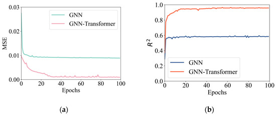
Figure 11.
Loss and correlation coefficient of the training set. (a) Description of the MSE of the two surrogate models during the training process. (b) Description of the R2 of the two surrogate models during the training process.
A test sample was randomly selected from the test set, and the DEPSO algorithm based on the surrogate model was used for history matching. The algorithm parameters were set to be the same as those in Case 1. There were a total of 57 fitting parameters in this process. Figure 12 displays the water-cut graphs for six wells after history matching using the DEPSO algorithm based on the GNT surrogate model. In the figure, the red dotted line represents the actual observed data, the green curve represents the predicted values from the updated model after history matching using the DEPSO hybrid optimization algorithm, and the gray curve represents the predicted data from the initial model ensemble. The distribution of the predicted data from the gray curve is relatively scattered. This is because the initial model ensemble was generated using the Gaussian simulation method, which is stochastic and leads to uncertainty in the initial stage of the model. Compared to the production curves obtained from the initial reservoir model, the target reservoir production curves obtained using the GNT-DEPSO method are closer to the actual observed data and have a higher degree of fit with the actual historical production data.
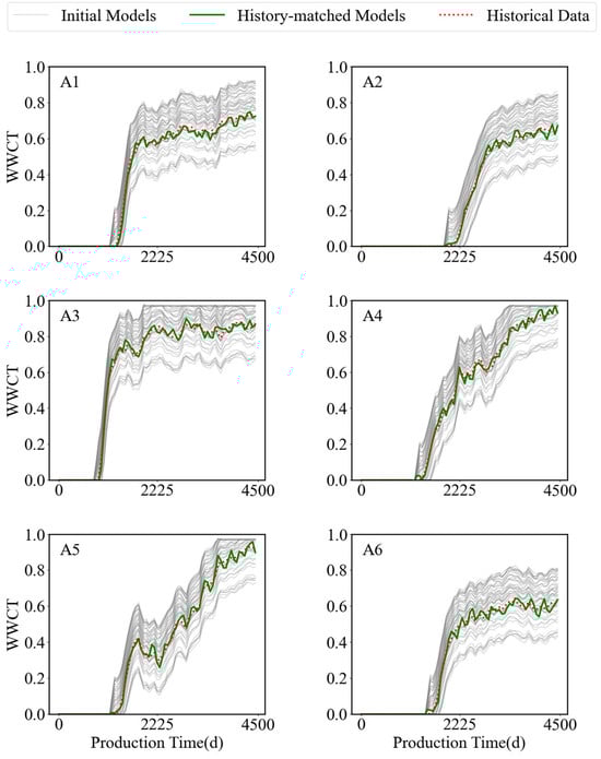
Figure 12.
Historical matching results of WWCT curves for 6 production wells using the GNT-DEPSO method.
A well was randomly selected, and comparison graphs of its conductivity and connected volume before and after history matching were plotted. The results are shown in Figure 13, Figure 14, Figure 15 and Figure 16. As shown in Figure 17, six production wells were randomly selected, and three optimization methods—DEPSO, PSO, and DE—were used for history matching. Each subplot contains three curves, representing the water-cut changes obtained using different optimization methods. In the figure, the red dotted line represents the historical water-cut data, and the green curve represents the predicted data optimized using the DEPSO algorithm. These data show a high degree of consistency with the historical data, indicating extremely high fitting accuracy. The orange and pink lines correspond to the predicted data from the DE and PSO algorithms, respectively, with their fitting accuracies decreasing in sequence.
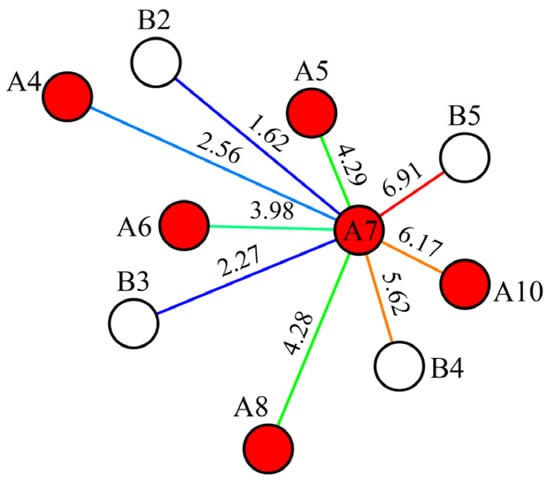
Figure 13.
Transmissibility before history matching. Here, red circles represent production wells, white circles represent injection wells, and letters are used to denote well names.
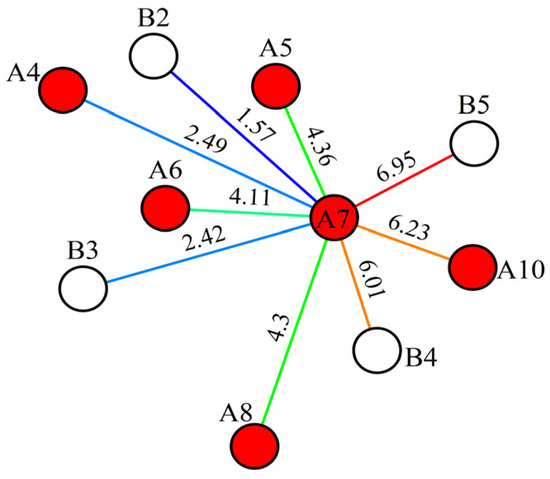
Figure 14.
Transmissibility after history matching. Here, red circles represent production wells, white circles represent injection wells, and letters are used to denote well names.
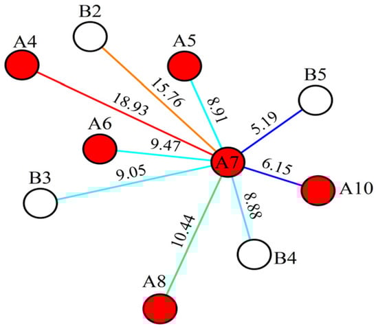
Figure 15.
Connection volume before history matching. Here, red circles represent production wells, white circles represent injection wells, and letters are used to denote well names.
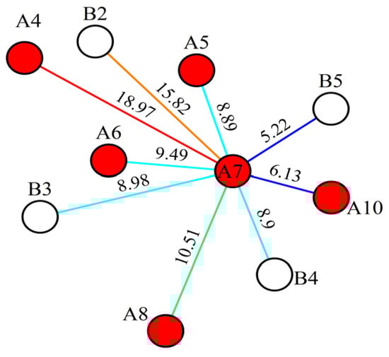
Figure 16.
Connection volume after history matching. Here, red circles represent production wells, white circles represent injection wells, and letters are used to denote well names.
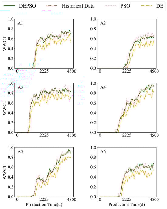
Figure 17.
Comparison of WWCT curve fitting using different algorithms.
Figure 18 illustrates the changes in WWCT before and after reservoir history matching, along with the predicted WWCT curve over the past 2000 days after history matching. A dashed line is used to mark the boundary between the pre- and post-fitting periods. The red line represents the WWCT changes after fitting, while the blue line represents the WWCT changes before fitting. It can be observed that the fitting results are satisfactory. For each production well, the correlation coefficient R2 between the predicted and actual water cut values is first calculated. Subsequently, the R2 values for all production wells are averaged to obtain the mean water-cut fitting accuracy for the entire set of production wells. Table 4 presents the WWCT fitting rates for all production wells in the reservoir model, with an average WWCT fitting rate of 87.8%.
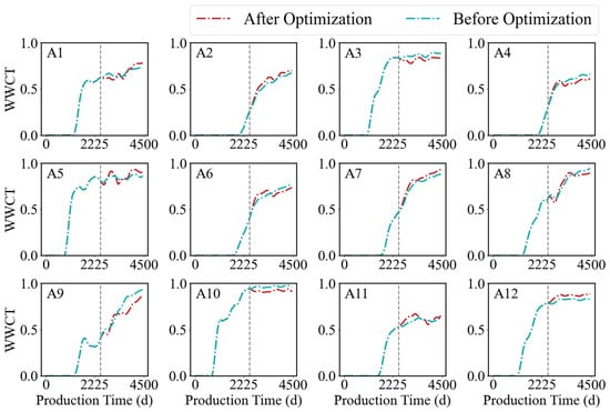
Figure 18.
Comparison of WWCT before and after fitting.
Table 4.
The fitting rate of WWCT in a single well.
4. Conclusions
In this study, based on research into the CRM model, we propose combining the GNT model with the CRM for use as a surrogate model in AHM. This model integrates multiple factors, such as reservoir well pattern distribution and production dynamics, and specifically considers the characteristics of interwell connectivity to predict the WWCT of production wells. To capture long-range dependencies in sequences, we introduce the Transformer into the model. Its attention mechanism can also focus on more critical nodes, reducing the impact of non-critical nodes on the model’s output. The model performs well during the training phase, with a correlation coefficient score exceeding 0.95. Using the GNT surrogate model, we invert the interwell connectivity parameters with DEPSO. The results from the numerical examples demonstrate that this fusion algorithm exhibits stronger global optimization capabilities and achieves significant history matching effects. When applying the proposed method to a complex case, the correlation coefficient score of the surrogate model approaches 0.93, and the single-well water-cut fitting rate reaches 87.8%. This not only verifies the feasibility and effectiveness of the method but also provides a new approach and technical means for reservoir history matching, which is expected to play an important role in the field of reservoir engineering.
Author Contributions
Methodology, B.L. (Botao Liu) and H.Z.; validation, T.X., B.L. (Bo Li) and Y.X.; formal analysis, B.L. (Botao Liu) and H.Z.; investigation, Y.X.; writing—original draft preparation, T.X. and B.L. (Bo Li); writing—review and editing, B.L. (Botao Liu), Y.X. and H.Z. All authors have read and agreed to the published version of the manuscript.
Funding
This research received no external funding.
Data Availability Statement
Data are available from the corresponding author.
Acknowledgments
This work was supported by The National Natural Science Foundation of China’s “Research on Interwell Fracturing Interference and Intelligent optimization for Anti Fracturing Interference in Shale Gas Reservoirs Based on Connection Element Method” (52474029); the Open Fund of Hubei Key Laboratory of Oil and Gas Drilling and Production Engineering (Yangtze University): Application Research of Machine Learning in Shale Gas Well Fluid Accumulation Prediction and Foam Drainage Applicability Diagnosis (YQZC202402); the project of young people in the Education Hall of Hubei (No.Q20161311); Research on Modeling and Optimal Control for Multi-Physical Field Coupling in Carbonate Reservoir (62273060).
Conflicts of Interest
The authors declare no conflicts of interest.
References
- Xu, Y.; Hu, Y.; Rao, X.; Zhao, H.; Zhong, X.; Peng, X.; Zhan, W.; Sheng, G.; Liu, D. A fractal physics-based data-driven model for water-flooding reservoir (FlowNet-fractal). J. Pet. Sci. Eng. 2022, 210, 109960. [Google Scholar] [CrossRef]
- Chai, Z.; Yan, B.; Killough, J.E.; Wang, Y. An efficient method for fractured shale reservoir history matching: The embedded discrete fracture multi-continuum approach. J. Pet. Sci. Eng. 2018, 160, 170–181. [Google Scholar] [CrossRef]
- Oliver, D.S.; Reynolds, A.C.; Liu, N. Inverse Theory for Petroleum Reservoir Characterization and History Matching; Cambridge University Press: Cambridge, UK, 2008. [Google Scholar]
- Chang, H.; Zhang, D. History matching of stimulated reservoir volume of shale-gas reservoirs using an iterative ensemble smoother. Spe J. 2018, 23, 346–366. [Google Scholar] [CrossRef]
- Chakra, N.C.C.; Saraf, D.N. History matching of petroleum reservoirs employing adaptive genetic algorithm. J. Pet. Explor. Prod. Technol. 2016, 6, 653–674. [Google Scholar] [CrossRef]
- Maschio, C.; Schiozer, D.J. Integration of geostatistical realizations in data assimilation and reduction of uncertainty process using genetic algorithm combined with multi-start simulated annealing. Oil Gas Sci. Technol. Rev. D’ifp Energ. Nouv. 2019, 74, 73. [Google Scholar] [CrossRef]
- Sun, Z.; Liu, Y.; Cai, H.; Gao, Y.; Jiang, R. The numerical simulation study on the dynamic variation of residual oil with water drive velocity in water flooding reservoir. Front. Energy Res. 2023, 10, 977109. [Google Scholar] [CrossRef]
- Kazemi, A.; Stephen, K.D. Schemes for automatic history matching of reservoir modeling: A case of Nelson oilfield in UK. Pet. Explor. Dev. 2012, 39, 349–361. [Google Scholar] [CrossRef]
- Li, B.; Bhark, E.W.; Billiter, T.C.; Dehghani, K. Best practices of assisted history matching using design of experiments. SPE J. 2019, 24, 1435–1451. [Google Scholar] [CrossRef]
- Forouzanfar, F.; Wu, X.-H. Constrained iterative ensemble smoother for multi solution search assisted history matching. Comput. Geosci. 2021, 25, 1593–1604. [Google Scholar] [CrossRef]
- Avansi, G.D.; Maschio, C.; Schiozer, D.J. Simultaneous history-matching approach by use of reservoir-characterization and reservoir-simulation studies. SPE Reserv. Eval. Eng. 2016, 19, 694–712. [Google Scholar] [CrossRef]
- Xu, W. Generalising History Matching for Enhanced Calibration of Computer Models; University of Exeter: Exeter, UK, 2021. [Google Scholar]
- Ma, X.; Zhang, K.; Zhang, J.; Wang, Y.; Zhang, L.; Liu, P.; Yang, Y.; Wang, J. A novel hybrid recurrent convolutional network for surrogate modeling of history matching and uncertainty quantification. J. Pet. Sci. Eng. 2022, 210, 110109. [Google Scholar] [CrossRef]
- Tang, M.; Liu, Y.; Durlofsky, L.J. A deep-learning-based surrogate model for data assimilation in dynamic subsurface flow problems. J. Comput. Phys. 2020, 413, 109456. [Google Scholar] [CrossRef]
- Xue, L.; Gu, S.; Mi, L.; Zhao, L.; Liu, Y.; Liao, Q. An automated data-driven pressure transient analysis of water-drive gas reservoir through the coupled machine learning and ensemble Kalman filter method. J. Pet. Sci. Eng. 2022, 208, 109492. [Google Scholar] [CrossRef]
- Saad, G.; Ghanem, R. Characterization of reservoir simulation models using a polynomial chaos-based ensemble Kalman filter. Water Resour. Res. 2009, 45, W04417. [Google Scholar] [CrossRef]
- Razavi, S.; Tolson, B.A.; Burn, D.H. Review of surrogate modeling in water resources. Water Resour. Res. 2012, 48, W07401. [Google Scholar] [CrossRef]
- Elsheikh, A.H.; Hoteit, I.; Wheeler, M.F. Efficient Bayesian inference of subsurface flow models using nested sampling and sparse polynomial chaos surrogates. Comput. Methods Appl. Mech. Eng. 2014, 269, 515–537. [Google Scholar] [CrossRef]
- Wang, L.; Yao, Y.; Luo, X.; Adenutsi, C.D.; Zhao, G.; Lai, F. A critical review on intelligent optimization algorithms and surrogate models for conventional and unconventional reservoir production optimization. Fuel 2023, 350, 128826. [Google Scholar] [CrossRef]
- Li, W.; Lin, G. An adaptive importance sampling algorithm for Bayesian inversion with multimodal distributions. J. Comput. Phys. 2015, 294, 173–190. [Google Scholar] [CrossRef]
- Zhang, J.; Man, J.; Lin, G.; Wu, L.; Zeng, L. Inverse modeling of hydrologic systems with adaptive multifidelity Markov chain Monte Carlo simulations. Water Resour. Res. 2018, 54, 4867–4886. [Google Scholar] [CrossRef]
- Ma, X.; Zhang, K.; Zhang, L.; Yao, C.; Yao, J.; Wang, H.; Jian, W.; Yan, Y. Data-driven niching differential evolution with adaptive parameters control for history matching and uncertainty quantification. Spe J. 2021, 26, 993–1010. [Google Scholar] [CrossRef]
- Qiao, P.; Wu, Y.; Ding, J.; Zhang, Q. A new sequential sampling method of surrogate models for design and optimization of dynamic systems. Mech. Mach. Theory 2021, 158, 104248. [Google Scholar] [CrossRef]
- Janatian, N. Real-Time Optimization and Control for Oil Production Under Uncertainty. Ph.D. Thesis, University of South-Eastern Norway, Notodden, Norway, 2024. [Google Scholar]
- Canchumuni, S.W.A.; Emerick, A.A.; Pacheco, M.A.C. History matching geological facies models based on ensemble smoother and deep generative models. J. Pet. Sci. Eng. 2019, 177, 941–958. [Google Scholar] [CrossRef]
- Qin, Z.; Jiang, A.; Faulder, D.; Cladouhos, T.T.; Jafarpour, B. Efficient optimization of energy recovery from geothermal reservoirs with recurrent neural network predictive models. Water Resour. Res. 2023, 59, e2022WR032653. [Google Scholar] [CrossRef]
- Liu, W.; Liu, W.D.; Gu, J. Forecasting oil production using ensemble empirical model decomposition based Long Short-Term Memory neural network. J. Pet. Sci. Eng. 2020, 189, 107013. [Google Scholar] [CrossRef]
- Aghayev, Z.; Voulanas, D.; Gildin, E.; Beykal, B. Surrogate-Assisted Optimization of Highly Constrained Oil Recovery Processes Using Classification-Based Constraint Modeling. Ind. Eng. Chem. Res. 2025, 64, 7619–7940. [Google Scholar] [CrossRef]
- Khormali, A.; Ahmadi, S. Synergistic effect between oleic imidazoline and 2-mercaptobenzimidazole for increasing the corrosion inhibition performance in carbon steel samples. Iran. J. Chem. Chem. Eng. Res. 2023, 42, 321–336. [Google Scholar]
- Liu, W.; Pyrcz, M.J. Physics-informed graph neural network for spatial-temporal production forecasting. Geoenergy Sci. Eng. 2023, 223, 211486. [Google Scholar] [CrossRef]
- Huang, Z.-Q.; Wang, Z.-X.; Hu, H.-F.; Zhang, S.-M.; Liang, Y.-X.; Guo, Q.; Yao, J. Dynamic interwell connectivity analysis of multi-layer waterflooding reservoirs based on an improved graph neural network. Pet. Sci. 2024, 21, 1062–1080. [Google Scholar] [CrossRef]
- Wang, H.; Han, J.; Zhang, K.; Yao, C.; Ma, X.; Zhang, L.; Yang, Y.; Zhang, H.; Yao, J. An interpretable interflow simulated graph neural network for reservoir connectivity analysis. SPE J. 2021, 26, 1636–1651. [Google Scholar] [CrossRef]
- Lu, G.; Zeng, L.; Dong, S.; Huang, L.; Liu, G.; Ostadhassan, M.; He, W.; Du, X.; Bao, C. Lithology identification using graph neural network in continental shale oil reservoirs: A case study in Mahu Sag, Junggar Basin, Western China. Mar. Pet. Geol. 2023, 150, 106168. [Google Scholar] [CrossRef]
- Huang, H.; Gong, B.; Sun, W. A deep-learning-based graph neural network-long-short-term memory model for reservoir simulation and optimization with varying well controls. SPE J. 2023, 28, 2898–2916. [Google Scholar] [CrossRef]
- Vaswani, A.; Shazeer, N.; Parmar, N.; Uszkoreit, J.; Jones, L.; Gomez, A.N.; Kaiser, Ł.; Polosukhin, I. Attention is all you need. In Proceedings of the Advances in Neural Information Processing Systems 30 (NIPS 2017), Long Beach, CA, USA, 4–9 December 2017; Volume 30. [Google Scholar]
- Gao, M.; Wei, C.; Zhao, X.; Huang, R.; Li, B.; Yang, J.; Gao, Y.; Liu, S.; Xiong, L. Intelligent optimization of gas flooding based on multi-objective approach for efficient reservoir management. Processes 2023, 11, 2226. [Google Scholar] [CrossRef]
- Yousef, A.A.; Gentil, P.; Jensen, J.L.; Lake, L.W. A capacitance model to infer interwell connectivity from production-and injection-rate fluctuations. SPE Reserv. Eval. Eng. 2006, 9, 630–646. [Google Scholar] [CrossRef]
- Scarselli, F.; Gori, M.; Tsoi, A.C.; Hagenbuchner, M.; Monfardini, G. The graph neural network model. IEEE Trans. Neural Netw. 2008, 20, 61–80. [Google Scholar] [CrossRef]
- Pei, Y.; Huang, T.; Van Ipenburg, W.; Pechenizkiy, M. ResGCN: Attention-based deep residual modeling for anomaly detection on attributed networks. Mach. Learn. 2022, 111, 519–541. [Google Scholar] [CrossRef]
- Shami, T.M.; El-Saleh, A.A.; Alswaitti, M.; Al-Tashi, Q.; Summakieh, M.A.; Mirjalili, S. Particle swarm optimization: A comprehensive survey. IEEE Access 2022, 10, 10031–10061. [Google Scholar] [CrossRef]
- Ibiam, E.; Geiger, S.; Demyanov, V.; Arnold, D. Optimization of polymer flooding in a heterogeneous reservoir considering geological and history matching uncertainties. SPE Reserv. Eval. Eng. 2021, 24, 19–36. [Google Scholar] [CrossRef]
- Santhosh, E.C.; Sangwai, J.S. A hybrid differential evolution algorithm approach towards assisted history matching and uncertainty quantification for reservoir models. J. Pet. Sci. Eng. 2016, 142, 21–35. [Google Scholar] [CrossRef]
- Lin, A.; Liu, D.; Li, Z.; Hasanien, H.M.; Shi, Y. Heterogeneous differential evolution particle swarm optimization with local search. Complex Intell. Syst. 2023, 9, 6905–6925. [Google Scholar] [CrossRef]
Disclaimer/Publisher’s Note: The statements, opinions and data contained in all publications are solely those of the individual author(s) and contributor(s) and not of MDPI and/or the editor(s). MDPI and/or the editor(s) disclaim responsibility for any injury to people or property resulting from any ideas, methods, instructions or products referred to in the content. |
© 2025 by the authors. Licensee MDPI, Basel, Switzerland. This article is an open access article distributed under the terms and conditions of the Creative Commons Attribution (CC BY) license (https://creativecommons.org/licenses/by/4.0/).